Optimal Pricing Policies with an Allowable Discount for Perishable Items under Time-Dependent Sales Price and Trade Credit

Abstract

Trade credit is generally used by businesses to obtain external funds. This article demonstrates an inventory system from the retailer’s point of view in which (1) the influence of trade credit on expanding small businesses and their consumers is the focus of this research, and (2) the retailer’s on-hand inventory follows the non-instantaneous deterioration. (3) To maximize profit, the demand is disclosed, which is based on not just the sales price, but also on cumulative demand, which indicates saturation and diffusion. (4) The product’s initial price and the permitted discount rate at the time of deterioration are considered to be time-dependent functions of the sales price. In the absence of deterioration, the item is sold at a constant rate, and whenever deterioration occurs, the sales price is assumed to be an exponential function of the discount variable. The main aim is to optimize the total profit of the retailer in terms of cycle time and sales price. The traditional algorithm of optimization is used to address the optimization problem. Finally, the theoretical results are validated by solving three numerical illustrations and conducting a sensitivity analysis of the main factors resulting from the following managerial implications: (1) credit period provides the maximum profit margin of any financing method, and (2) an increase in the initial rate of demand raises sales price while increasing overall profit significantly.

1. Introduction

1.1. Overview and Practical Motivations

In recent transactions, economic order policy is widely used in any business transaction to increase the profitability level [1]. In addition, trade credit is now a prominent kind of financing being commonly implemented in business. Trade credit research has expanded from the domain of banking and finance to become a multidisciplinary scientific topic with significant contributions from business management, operations research, production and finance, economics, and other disciplines [2]. Many firms now have deals with credit card corporations and a strategy of interest-free installment to offer their consumers a limited time to gain market share. To maximize total profit, businesses must analyze the trade-off between credit risks and the income potential of a marginal sale. This article uses a mathematical technique to evaluate the influence and value of trade credit on the growth of small retailers and their customers.

In real life, deterioration is a natural phenomenon in inventory control [3,4]. The implication of deterioration has been highlighted due to scientific aspects. Items such as electronics, fuel, blood, and cereals begin to degrade after a certain length of time and lose their originality [5]. The term “non-deterioration period” is used in this article to describe the period during which items in a lot are non-deteriorative [6,7,8,9]. In other words, this is the period during which the goods in the same lot have a minimum shelf life. During the non-deterioration phase, inventory decline is only due to demand; however, after the non-deterioration time, the inventory decreases due to both demand and deterioration [10]. This research particularly develops a model for electronic goods which can be considered “non-instantaneous deteriorating items”.

Recent technology advancements, such as online marketing, electronic shelf, and labeling, have permitted dynamic pricing strategies across a wide range of businesses [11,12]. The company can decrease its losses by using various marketing strategies and promotional tools, such as a discount policy. Customers like to buy when there are discounts available. Therefore, the discount strategy is also considered in this model.

Consumer demand is affected by both the product’s life and its sales price. The demand rate in traditional inventory models is assumed to be constant, unaffected by sales price, time, and inventory levels, which is not the case in reality. The sales price has a huge influence on demand, and companies such as Ford and Dell Computer have used dynamic pricing in conjunction with manufacturing and distribution strategies to increase profitability [13,14]. The demand for a product decrease with time in areas such as electronics and fashion design [15], and when a new product is introduced to the market, consumers want to buy it based on its features. However, as technology advances and new features are added to that model, the demand for the previous model decreases over time. Customers were unhappy when Amazon initially tried dynamic pricing on DVDs, and when they realized they were being charged more than others for the same products, they demanded an apology and refund from Amazon [16]. The demand for items is influenced not just by the item’s sale price, but also by the overall demand or sale of the item. Hence, the companies are facing challenges as a result of supermarket dynamics and product features. Therefore, a strong technique is to think about the dynamic pricing function of demand where the demand is fluctuating according to customer demand. The study is motivated by these factors and instead of using a fixed sales price, a dynamic pricing approach is more successful in terms of increasing revenue.

1.2. Aim of This Study

This study focuses on the following research problems under decision-maker/retailer behavior and the dynamic effects of supply level:

• What would be the best pricing methods for perishable products which optimize the total profit?
• What would be the optimal sales price of a product when it depends on the time?
• What would be the optimal cycle time which optimizes the total profit?
• Under the dynamic demand with the assumption of time-varying holding cost, how much inventory should be supplied and in what quantities?
• If the retailer collects a trade credit period from the supplier, then what would be the effects on total profit?
• Which behavior is preferred by the retailer and how do the model’s key parameters influence this preference?
• What would be the managerial implications of implementing this model to use in reality?

1.3. Flow of the Paper

To address the above research questions, realistic scenarios formed the base of this work, and the subsequent sections of the current model are accessible as follows. In Section 2, the existing literature is reviewed. The notation and assumptions are displayed in Section 3. For a proposed problem, the derivation of a mathematical model is discussed in Section 4. Section 5 gives an algorithm to test the optimality of a retailer’s overall profit function. Section 6 discusses numerical illustrations for each situation, sensitivity analysis of main parameters, and managerial implications. The conclusions and future possibilities are deliberated in Section 7.

2. Literature Review

This research is relevant to three research areas: the research of the trade credit models, models of non-instantaneous perishable items in inventory, and dynamic pricing models. The use of trade credit may significantly improve operational efficiency. Inventory policies have been thoroughly focused on the concept of trade credit finance. In the actual world, cash on delivery is impractical. Therefore, permissible delay in payment strategy becomes a more communal payment method in real-world company dealings. Initially in [1], the optimal inventory policy with the impact of the trade credit strategy is explored. In [2], the inventory system with the trade credit policy under an imperfect green production environment is examined. In [3], joint dynamic pricing and investment strategy for perishable foods with price–quality dependent demand is formulated. For perishable items, in [4], optimal dynamic pricing and preservation technology investment with reference to the price effects are proposed. Under trade credit policy, shortages, and sales-price-dependent demand, a model with deterioration goods with a non-instantaneous rate is designed in [5]. A mathematical model is constructed in [17], with the assumption of non-linear holding cost under trade credit. In [18], an analysis of the optimal portfolio on finite and small-time horizons for a stochastic volatility market model is developed. In [19], a model with a supply chain, where buyers have access to trade credit provided by an upstream vendor is designed.

In [20], the concept of “non-instantaneous deterioration” is firstly described. Following that, researchers concentrated on the inventory issues of non-instantaneous perishable units in numerous situations. In [21], the inventory model for perishable items is reviewed. In [6], a mathematical model under time-varying holding expense for perishable inventory is suggested. Contributions to inventory systems are highlighted by terms such as discount strategy, back ordering, trade credit, and lost sale; the best joint replenishment strategy for several non-instantaneously decaying products is designed in [7]. In [8], a mathematical model for a non-instantaneously perishable rate under carbon emission restrictions is introduced. In [9], a mathematical model for non-instantaneous perishable inventory under the investment in preservation technology is developed. Further, in [22], the influence of continuous deterioration in an inventory model to assess just-in-time agreement is analyzed. Recently, in [23], the pricing strategy for a perishable inventory with a non-instantaneous rate, where the demand is selling price and freshness dependent investigated. Under price-advertisement-dependent demand, in [10], an inventory strategy for perishable inventory with a non-instantaneous rate with trade credit policy and time value of money is developed.

For the notion of a dynamic strategy of pricing for perishable units, there is a rising amount of effective literature. In [11], for perishable items, a dynamic pricing model by selling a finite-time-horizon supply of goods is analyzed. A mathematical model for perishable inventory is proposed in [12] under a dynamic pricing policy. In [13], a dynamic demand with multi-product and a stochastic inventory model is analyzed. A dynamic demand model is introduced in [14] with a stock-out dependency. In [24], a dynamic pricing problem is considered for deteriorating goods about a reference price. This approach is designed to optimize overall profit while recognizing that demand is influenced by both current and historical prices. Further, in [25], joint dynamic pricing and inventory control policy for a stochastic inventory system with perishable products is developed. The use of stochasticity in the mathematical model also plays an important role and in [26], the problem of portfolio optimization in a simple incomplete market for small-time horizons is discussed. In [15], a model for firms dealing with product returns is developed, and the paper discusses dynamic pricing and the resale of products in perfect condition. Further, in [27], the impact of decision parameters advertising and expected delivery time on the desire for dual supply chain setups driven by the manufacturer is investigated. Recently, a dynamic demand model, in which the demand is influenced by the time-varying function of the sales price and also by cumulative demand is analyzed in [28]. In [29], dynamic pricing and inventory policies in a food supply chain of growing and deteriorating items is investigated. In Table 1, the contributions of the existing survey are abridged.

Table 1. Gap identification and summary of previous work for this work.

Author(s)	Demand Type	Non-Instantaneous Deterioration	Variable Holding Cost	Trade Credit	Nature of Sales Price
[8]	Fuzzy price-sensitive	Yes	No	Yes	Linear
[9]	Price-sensitive	Yes	No	No	Constant
[11]	Non-homogeneous	No	No	No	Dynamic price
[25]	Dynamic Pricing	No	No	No	Time dependent
[28]	Dynamic pricing	Yes	Yes	No	Constant and time dependent
In this paper	Dynamic pricing	Yes	Yes	Yes	Constant and time dependent

Research Gap and Contributions

Based on the literature survey and from the above Table, several studies have been conducted on different mixtures, but the uniqueness of this article is that all the combinations are investigated which were previously not considered in any model. The most similar work to this article is [28], but in terms of trade credit policy, this paper significantly differs, which is the novelty of this work, and in the current scenario, permissible delay in payment policy plays an important role for any company or organization and also helps the retailer to earn more revenue. Therefore, this paper extends [28] by adding the upstream trade credit policy between the supplier and the retailer.

The following are the important contributions of this article:

• This study addresses a policy with non-instantaneous perishable units with a time-varying sales price and a permitted discount rate for items that deteriorate after a certain period.
• The model is used to evaluate variable holding cost, as they increase over time, as well as to manage perishable commodities to prevent spoilage.
• The rate of demand for an item is determined not only by the product’s sales price, but also by the cumulative demand or sale.
• In contrast to many situations, this model maximizes the overall profit under the trade credit policy.
• To determine the optimality of the total profit function, this model employs the traditional optimization approach.
• To demonstrate the theoretical outcomes, this article discusses the numerical illustrations for each situation under trade credit.
• This study analyzes the sensitivity analysis of the main parameters and managerial implications, which gives the best strategy to the retailer for maximizing total profit.

3. Problem Explanation, Notation, and Assumptions

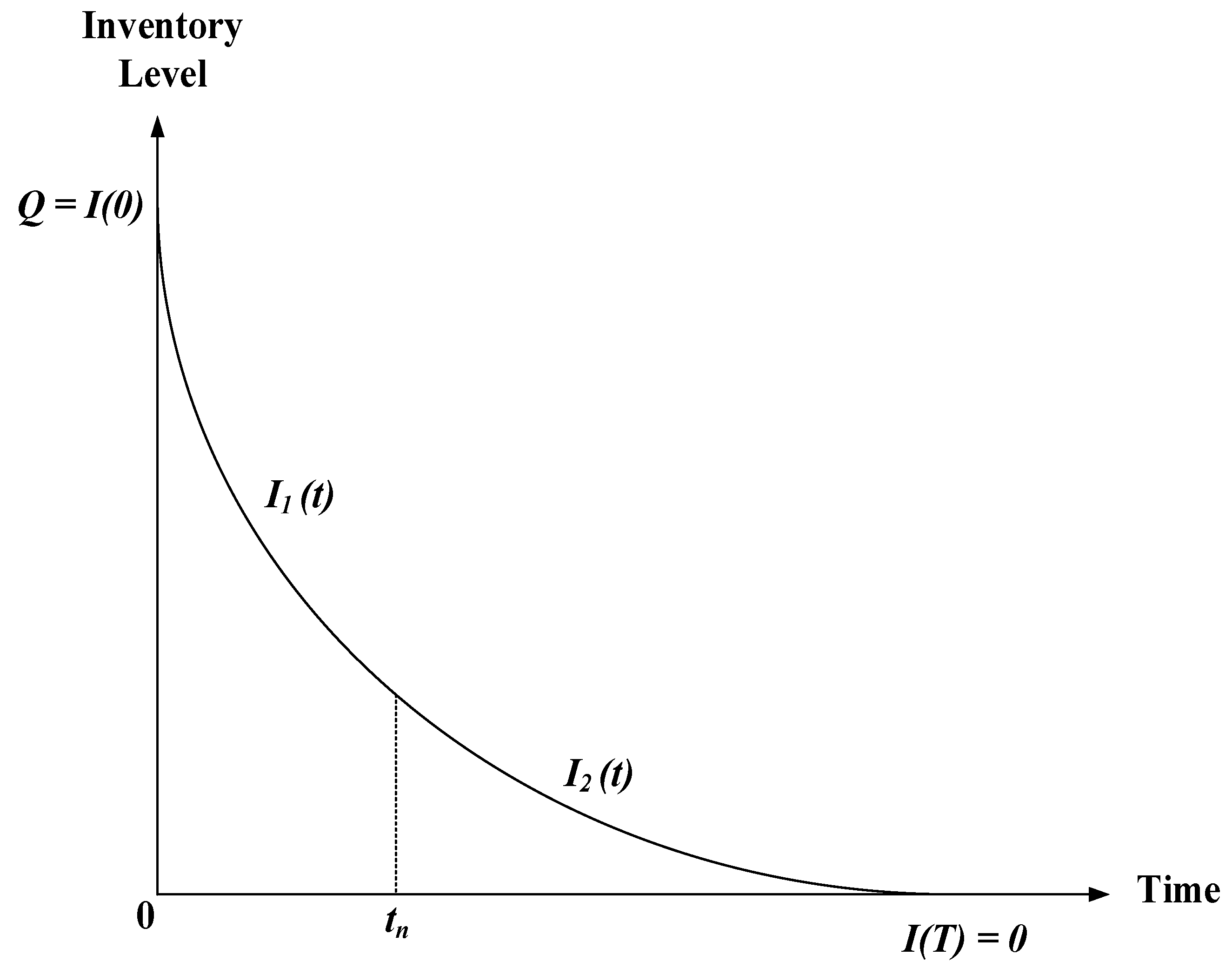
3.1. Problem Explanation

In this article, a dynamic pricing policy is investigated under permissible delay in payment for perishable items with a non-instantaneous rate, in which the company suffers spoilage difficulties, and instead of a constant sale price, the retailer may provide variations with the appropriate discount during the period of spoilage. A company may adjust the price over time, especially if a customer’s demand is sensitive to price. This is a real-life situation for many businesses around the world. The model investigates the dynamic demand for perishable products and examines the trade credit policy situation since it benefits the company and helps the retailer to increase sales. In a real-world inventory scenario, developing a realistic mathematical model that incorporates information with accuracy and certainty is extremely challenging. The focus of this article, however, is to create a model that would be used to connect real-life situations.

3.2. Assumptions

• The current inventory system is limited to a single product.
• The rate of deterioration is considered to be non-instantaneous. That is, during the period $\left(0,t_n\right)$, the items in inventory are non-deteriorating and at that time $t_n$, the deterioration begins in the system, and items deteriorate at a constant rate ${\theta }_n$ [8,10].
• When the deterioration begins in the system, per unit time, throughout $\left(t_n,T\right)$, the holding cost is presumed to be time varying and is defined by $h\left(t\right)=h+\tau \left(t-t_n\right)$, where $h$ is the holding cost parameter and $\tau$ is the rate of increase over time (one can examine an article’s assumption [28]).
• The sales price of the product is assumed to be constant $S$; when there is no deterioration during $\left(0,t_n\right)$ and when the deterioration begin in the system, it is assumed to be exponential decreasing function of time with variable discount $\omega$ during $\left(t_n,T\right)$ (one can examine an article’s assumption [28]. Therefore, the time-dependent sales price is described as $S\left(t\right)=\{\begin{array}{l}S;\hspace{1em}0\le t\le t_n\\ S \exp \left(-\omega \left(t-t_n\right)\right);\hspace{1em}{t}_n\le t\le T\end{array}$
• The dynamic demand rate $D\left(S,t\right)=\{\begin{array}{l}{D}_1\left(S,t\right);\hspace{1em}0<t<t_n\\ D_2\left(S,t\right);\hspace{1em}{t}_n<t<T\end{array}$ is considered to be a function of the sales price and also cumulative demand, which can be defined as follows:
• When there is no deterioration, the rate of demand can be determined as $\frac{d{D}_1\left(S,t\right)}{dt}=a-bS-\psi D_1\left(S,t\right)$
• When deterioration begins in the system, the rate of demand can be determined as $\frac{d{D}_2\left(S,t\right)}{dt}=a-bS \exp \left(-\omega \left(t-t_1\right)\right)-\psi D_2\left(S,t\right)$
• Where $a$ represents a scaling demand, $b$ represents the sensitivity of the demand concerning price, and both of them are known and positive. The parameter $\eta$ is the reduced rate of sales, which indicates the saturation impact and includes the percentage of the market that will not buy the units at the specified period one can examine an article’s assumption [28].
• The retailer obtains years of credit period from the supplier, where the retailer can pay after $M$ and will make the interest $\left(I_g\right)$ throughout the interval from 0 to $M$ and will pay back the interest (I_p) throughout the interval from $M$ to $T$ [3,18].
• With a lead time of zero, the rate of replenishment is infinite.
• The retailer trades only a single kind of deteriorating item, and no replacement is admissible throughout the entire cycle time.
• Shortages are not permitted.

4. Mathematical Model

This section frames a mathematical model for perishable items with a non-instantaneous rate under the dynamic demand rate, which is the function of the time-dependent sales price and cumulative demand. The inventory system is shown in Figure 1.

Figure 1. The inventory system and proposed problem (Adapted from [28]).

By the commencement of per cycle, initial $Q$ units reach the organization, and the inventory system reveals no deterioration over the period from 0 to $t_n$. As a result, the quantity continues to decrease owing to the demand, and in this situation, the sales price of the item is constant and defined as $S\left(t\right)=S$. Thus, the rate of change in the demand $\left(0,t_n\right)$ is administered by the following equation:

$$\frac{d{D}_1\left(S,t\right)}{dt}=a-bS-\psi D_1\left(S,t\right)$$

(1)

with initial condition $D_1\left(S,0\right)=D_0$.

By solving (1) with the initial condition, the dynamic demand rate for non-deteriorating items is given by

$$D_1\left(S,t\right)=\exp \left(-\psi t\right)\left(D_0-\frac{a-bS}{\psi }\right)+\frac{a-bS}{\psi }$$

(2)

Now, at the time $t_n$, the units begin to deteriorate constantly, and deterioration occurs in the sales period $\left(t_n,T\right)$; which results in a decreasing utility or physical quantity from the original one. However, the decrease in utility can be transformed into a reduction in quantity while modeling. Therefore, during this period, the quantity continues to reduce owing to the joint impact of demand and deterioration. To increase the sales of the units, the sales price of the product is an exponentially decreasing function of time with variable discount and is given by $S\left(t\right)=S\exp \left(-\omega \left(t-t_n\right)\right)$. Thus, the following equation governs the rate of change in demand during the period $\left(t_n,T\right)$

$$\frac{d{D}_2\left(S,t\right)}{dt}=a-bS\exp \left(-\omega \left(t-t_n\right)\right)-\psi D_2\left(S,t\right)$$

(3)

with boundary condition $D_2\left(S,t_n\right)=D_1\left(S,t_n\right)$.

By solving Equation (3) with boundary condition, the dynamic demand rate for deteriorating items is determined as

$$D_2\left(S,t\right)=\frac{\exp \left(-\psi t\right)}{\psi \left(\omega -\psi \right)}\left(\begin{array}{l}-\psi \left(\exp \left(-\omega \left(t_n-t\right)+\psi t\right)\left(a-bS\right)\right)+D_0\omega \psi -\\ D_0{\psi }^2\left(a-bS\right)\left(\psi -\omega +\omega \exp \left(\psi t_n\right)\right)\end{array}\right)$$

(4)

Next, by following Equation (4), the inventory level for deteriorating items $\left(t_n,T\right)$ is denoted by $I_2\left(t\right)$, and at $t=T$, the level of inventory vanishes. However, the deterioration rate is measured to be a constant and is given by ${\theta }_n{I}_2\left(t\right)$. Thus, the inventory variances for this period are described as

$$\frac{d{I}_2\left(t\right)}{dt}=-D_2\left(S,t\right)-{\theta }_n{I}_2\left(t\right)$$

(5)

under the boundary condition $I_2\left(T\right)=0$.

By solving Equation (5), the level of inventory $\left(t_n,T\right)$ is defined as

$$I_2\left(t\right)=\frac{\exp \left(-{\theta }_{n}t\right)}{\psi \left(\omega -\psi \right)}\left(\begin{array}{l}\frac{\omega \left(a-bS\right)\left(\exp \left(\left(t_n-t\right)\psi +{\theta }_{n}t\right)-\exp \left(\left(t_n-T\right)\psi +{\theta }_{n}T\right)\right)}{{\theta }_n-\psi }-\\ \frac{\psi \left(a-bS\right)\left(\exp \left(t_n-t\right)\omega +{\theta }_{n}t\right)-\exp \left(\left(t_n-T\right)\omega +{\theta }_{n}T\right)}{{\theta }_n-\omega }-\\ \frac{\left(\omega -\psi \right)\left(D_0\psi +a-bS\right)\exp \left(t\left({\theta }_n-\psi \right)\right)-\exp \left({\theta }_n-\psi \right)}{{\theta }_n-\psi }\end{array}\right)$$

(6)

Now, the level of inventory for non-deteriorating items during the period $\left(0,t_n\right)$ is denoted by $I_1\left(t\right)$. Thus, the inventory variances for this period are described as

$$\frac{d{I}_1\left(t\right)}{dt}=-D_1\left(S,t\right)$$

(7)

and following Equation (6) and the use of continuity $I_1\left(t_n\right)=I_2\left(t_n\right)$ (see Figure 1) gives the boundary condition:

$$I_1\left(t_n\right)=\frac{\exp \left(-{\theta }_n{t}_n\right)}{\psi \left(\omega -\psi \right)}\left(\begin{array}{l}\left(\frac{\omega }{{\theta }_n-\psi }-\frac{\psi }{{\theta }_n-\omega }\right)\left(\begin{array}{l}\left(a-bS\right)\exp \left({\theta }_n{t}_n\right)-\\ \left(a-bS\right)\exp \left(\left(t_n-T\right)\psi +{\theta }_{n}T\right)\end{array}\right)\\ +\frac{\left(\omega -\psi \right)\left(D_0\psi +a-bS\right)}{{\theta }_n-\psi }\left(\exp \left({\theta }_n-\psi \right)-\exp \left(t_n\left({\theta }_n-\psi \right)\right)\right)\end{array}\right)$$

(8)

Thus, by solving Equation (7) with Equation (8), the inventory level for the period $\left(0,t_n\right)$ is defined as

$$\begin{array}{l}{I}_1\left(t\right)=\frac{\exp \left(-\eta t\right)\left(D_0\psi +a-bS\right)}{{\omega }^2}-\frac{\left(a-bS\right)t}{\psi }-\frac{\exp \left(-\psi t_n\right)\left(D_0\psi +a-bS\right)}{{\psi }^2}\\ +\frac{\left(a-bS\right)t_n}{\psi }+\frac{\exp \left(-{\theta }_n{t}_n\right)}{\eta \left(\omega -\eta \right)\left(\eta -{\theta }_n\right)\left(\omega -{\theta }_n\right)}\\ \left(\begin{array}{l}-\exp \left({\theta }_n{t}_n\right)b{\omega }^{2}S+\exp \left({\theta }_n{t}_n\right)b{\omega }^{2}S+\exp \left(t_n\left({\theta }_n-\psi \right)\right)D_0{\omega }^2\psi -\\ \exp \left(t_n\left({\theta }_n-\psi \right)\right)D_0\omega {\psi }^2+\exp \left(t_n\left({\theta }_n-\psi \right)\right)D_0{\omega }^2{\theta }_n+\exp \left(t_n\left({\theta }_n-\psi \right)\right)b{\omega }^{2}S+\\ \exp \left(\left(t_n-T\right)\psi +{\theta }_{n}T\right)b{\omega }^{2}S-\exp \left(\left(t_n-T\right)\omega +{\theta }_{n}T\right)b{\omega }^{2}S-\\ \exp \left(T\left({\theta }_n-\psi \right)\right)D_0{\omega }^2\psi -\exp \left(T\left({\theta }_n-\psi \right)\right)D_0\omega {\psi }^2-\exp \left(T\left({\theta }_n-\psi \right)\right)D_0{\omega }^2{\theta }_n-\\ \exp \left(T\left({\theta }_n-\psi \right)\right)b{\omega }^{2}S-\exp \left({\theta }_n{t}_n\right)a\omega \theta +\exp \left({\theta }_n{t}_n\right)a\psi {\theta }_n+\exp \left(t_n\left({\theta }_n-\psi \right)\right)a\omega \psi +\\ \exp \left(t_n\left({\theta }_n-\psi \right)\right)a\omega {\theta }_n-\exp \left(t_n\left({\theta }_n-\psi \right)\right)a\psi {\theta }_n+\exp \left(\left(t_n-T\right)\omega +{\theta }_{n}T\right)a\omega {\theta }_n-\\ \exp \left(\left(t_n-T\right)\omega +{\theta }_{n}T\right)a\psi {\theta }_n-\exp \left(T\left({\theta }_n-\psi \right)\right)a\psi \omega -\exp \left(T\left({\theta }_n-\psi \right)\right)a\omega {\theta }_n+\\ \exp \left(T\left({\theta }_n-\psi \right)\right)a\psi {\theta }_n+\exp \left({\theta }_n{t}_n\right)a{\omega }^2-\exp \left({\theta }_n{t}_n\right)a{\psi }^2-\exp \left(t_n\left({\theta }_n-\psi \right)\right)a{\omega }^2-\\ \exp \left(\left(t_n-T\right)\psi +{\theta }_{n}T\right)a{\omega }^2+\exp \left(\left(t_n-T\right)\omega +{\theta }_{n}T\right)a{\psi }^2+\exp \left(T\left({\theta }_n-\psi \right)\right)a{\omega }^2+\\ \exp \left({\theta }_n{t}_n\right)b\omega S{\theta }_n-\exp \left({\theta }_n{t}_n\right)b\psi S{\theta }_n-\exp \left(t_n\left({\theta }_n-\psi \right)\right)D_0\omega \psi {\theta }_n-\\ \exp \left(t_n\left({\theta }_n-\psi \right)\right)b\psi \omega S-\exp \left(t_n\left(\theta -\psi \right)\right)b\omega S{\theta }_n+\exp \left(t_n\left(\theta -\psi \right)\right)b\psi S{\theta }_n-\\ \exp \left(\left(t_n-T\right)\psi +{\theta }_{n}T\right)b\omega S{\theta }_n+\exp \left(\left(t_n-T\right)\omega +{\theta }_{n}T\right)b\psi S{\theta }_n+\exp \left(T\left({\theta }_n-\psi \right)\right)D_0\omega \psi {\theta }_n+\\ \exp \left(T\left({\theta }_n-\psi \right)\right)b\psi \omega S+\exp \left(T\left({\theta }_n-\psi \right)\right)b\omega S{\theta }_n-\exp \left(T\left({\theta }_n-\psi \right)\right)b\psi S{\theta }_n\end{array}\right)\end{array}$$

(9)

and by using the initial condition $I_1\left(0\right)=Q$ and following Equation (9), the optimal order quantity is obtained as

$$\begin{array}{l}Q=\frac{\left(D_0\psi +a-bS\right)}{{\omega }^2}-\frac{\exp \left(-\psi t_n\right)\left(D_0\psi +a-bS\right)}{{\psi }^2}+\frac{\left(a-bS\right)t_n}{\psi }+\frac{\exp \left(-{\theta }_n{t}_n\right)}{\eta \left(\omega -\eta \right)\left(\eta -{\theta }_n\right)\left(\omega -{\theta }_n\right)}\\ \left(\begin{array}{l}-\exp \left({\theta }_n{t}_n\right)b{\omega }^{2}S+\exp \left({\theta }_n{t}_n\right)b{\omega }^{2}S+\exp \left(t_n\left({\theta }_n-\psi \right)\right)D_0{\omega }^2\psi -\\ \exp \left(t_n\left({\theta }_n-\psi \right)\right)D_0\omega {\psi }^2+\exp \left(t_n\left({\theta }_n-\psi \right)\right)D_0{\omega }^2{\theta }_n+\exp \left(t_n\left({\theta }_n-\psi \right)\right)b{\omega }^{2}S+\\ \exp \left(\left(t_n-T\right)\psi +{\theta }_{n}T\right)b{\omega }^{2}S-\exp \left(\left(t_n-T\right)\omega +{\theta }_{n}T\right)b{\omega }^{2}S-\\ \exp \left(T\left({\theta }_n-\psi \right)\right)D_0{\omega }^2\psi -\exp \left(T\left({\theta }_n-\psi \right)\right)D_0\omega {\psi }^2-\exp \left(T\left({\theta }_n-\psi \right)\right)D_0{\omega }^2{\theta }_n-\\ \exp \left(T\left({\theta }_n-\psi \right)\right)b{\omega }^{2}S-\exp \left({\theta }_n{t}_n\right)a\omega \theta +\exp \left({\theta }_n{t}_n\right)a\psi {\theta }_n+\exp \left(t_n\left({\theta }_n-\psi \right)\right)a\omega \psi +\\ \exp \left(t_n\left({\theta }_n-\psi \right)\right)a\omega {\theta }_n-\exp \left(t_n\left({\theta }_n-\psi \right)\right)a\psi {\theta }_n+\exp \left(\left(t_n-T\right)\omega +{\theta }_{n}T\right)a\omega {\theta }_n-\\ \exp \left(\left(t_n-T\right)\omega +{\theta }_{n}T\right)a\psi {\theta }_n-\exp \left(T\left({\theta }_n-\psi \right)\right)a\psi \omega -\exp \left(T\left({\theta }_n-\psi \right)\right)a\omega {\theta }_n+\\ \exp \left(T\left({\theta }_n-\psi \right)\right)a\psi {\theta }_n+\exp \left({\theta }_n{t}_n\right)a{\omega }^2-\exp \left({\theta }_n{t}_n\right)a{\psi }^2-\exp \left(t_n\left({\theta }_n-\psi \right)\right)a{\omega }^2-\\ \exp \left(\left(t_n-T\right)\psi +{\theta }_{n}T\right)a{\omega }^2+\exp \left(\left(t_n-T\right)\omega +{\theta }_{n}T\right)a{\psi }^2+\exp \left(T\left({\theta }_n-\psi \right)\right)a{\omega }^2+\\ \exp \left({\theta }_n{t}_n\right)b\omega S{\theta }_n-\exp \left({\theta }_n{t}_n\right)b\psi S{\theta }_n-\exp \left(t_n\left({\theta }_n-\psi \right)\right)D_0\omega \psi {\theta }_n-\\ \exp \left(t_n\left({\theta }_n-\psi \right)\right)b\psi \omega S-\exp \left(t_n\left(\theta -\psi \right)\right)b\omega S{\theta }_n+\exp \left(t_n\left(\theta -\psi \right)\right)b\psi S{\theta }_n-\\ \exp \left(\left(t_n-T\right)\psi +{\theta }_{n}T\right)b\omega S{\theta }_n+\exp \left(\left(t_n-T\right)\omega +{\theta }_{n}T\right)b\psi S{\theta }_n+\exp \left(T\left({\theta }_n-\psi \right)\right)D_0\omega \psi {\theta }_n+\\ \exp \left(T\left({\theta }_n-\psi \right)\right)b\psi \omega S+\exp \left(T\left({\theta }_n-\psi \right)\right)b\omega S{\theta }_n-\exp \left(T\left({\theta }_n-\psi \right)\right)b\psi S{\theta }_n\end{array}\right)\end{array}$$

(10)

Next, the retailer received years of credit period and may face three situations throughout the entire cycle time $T$, the situations are: (1) $0<M<t_n<T$, (2) $0<t_n<M<T$, and (3) $0<t_n<T<M$. The interest gained $I_g$ and the interest paid $I_p$ for each situation by the retailer is discussed in the following Table 2.

Table 2. Interest gained and interest paid by the retailer for each situation.

Situations	Interest Gained (Ig)	Interest Paid (Ip)
$0<M<t_n<T$	The retailer gains the interest during the time from 0 to $M$ and that can be evaluated as $I{E}_1=S{I}_g{\displaystyle \underset{0}{\overset{M}{\int }}t{D}_1\left(S,t\right)dt}$	The retailer must pay the interest to the supplier during the time from $M$ to $T$, and that can be evaluated as $I{P}_1=P{I}_p\left({\displaystyle \underset{M}{\overset{t_n}{\int }}{I}_1\left(t\right)dt+{\displaystyle \underset{t_n}{\overset{T}{\int }}{I}_2\left(t\right)dt}}\right)$
$0<t_n<M<T$	The retailer gains the interest during the time from 0 to $t_n$ as well as from $t_n$ to $M$ and that can be evaluated as $I{E}_2=S{I}_g\left({\displaystyle \underset{0}{\overset{t_n}{\int }}t{D}_1\left(S,t\right)dt+{\displaystyle \underset{t_n}{\overset{M}{\int }}t{D}_2\left(S,t\right)dt}}\right)$	Same as the above case, the retailer must charge the interest to the supplier during the time from $M$ to $T$, and that can be evaluated as $I{P}_2=P{I}_p\left({\displaystyle \underset{M}{\overset{T}{\int }}{I}_2\left(t\right)dt}\right)$
$0<t_n<T<M$	The retailer gains the maximum profit as the credit period $M$ occurs after the completion of the entire cycle time and earns the additional interest during the period from $T$ to $M$, which can be evaluated as $\begin{array}{l}I{E}_3=S{I}_g\left({\displaystyle \underset{0}{\overset{t_n}{\int }}t{D}_1\left(S,t\right)dt+{\displaystyle \underset{t_n}{\overset{M}{\int }}t{D}_2\left(S,t\right)dt}}\right)+\\ S{I}_g\left(M-T\right)\left({\displaystyle \underset{0}{\overset{t_n}{\int }}{D}_1\left(S,t\right)dt+{\displaystyle \underset{t_n}{\overset{M}{\int }}{D}_2\left(S,t\right)dt}}\right)\end{array}$	The retailer has sold all the purchased goods from the supplier, hence the interest charged to the retailer will be zero. That is, $I{P}_3=0$

Now, the generated revenue of sales, throughout the cycle time $T$, is evaluated as

$$SR={\displaystyle \underset{0}{\overset{t_n}{\int }}S{D}_1\left(S,t\right)dt+{\displaystyle \underset{t_n}{\overset{T}{\int }}S\exp \left(-\omega \left(t-t_n\right)\right)D_2\left(S,t\right)dt}}$$

(11)

and total cost components are covered as shown below:

• Cost of ordering (per order): $OC=O$
• Cost of purchasing (per unit): $PC=PQ$
• Cost of holding (per unit time): $HC={\displaystyle \underset{0}{\overset{t_n}{\int }}h{I}_1\left(t\right)dt+{\displaystyle \underset{t_n}{\overset{T}{\int }}\left(h+\tau \left(t-t_n\right)\right)}{I}_2\left(t\right)dt}$
• Disposing cost (per unit): $DC=P_d{\displaystyle \underset{t_n}{\overset{T}{\int }}{\theta }_n{I}_2\left(t\right)dt}$

Therefore, per cycle time $T$, the retailer’s overall profit function, for all situations is given by

$$T{P}_i(S,T)=\frac{1}{T}\left(SR-OC-HC-PC-DC+I{E}_i-I{P}_i\right);\hspace{1em}i=1,2,3$$

That is,

$$T{P}_i(S,T)=\{\begin{array}{l}T{P}_1(S,T)\hspace{1em}if\hspace{1em}0<M<t_n<T\\ T{P}_2(S,T)\hspace{1em}if\hspace{1em}0<t_n<M<T\\ T{P}_3(S,T)\hspace{1em}if\hspace{1em}0<t_n<T<M\end{array}$$

(12)

in which

$$\begin{array}{l}T{P}_1(S,T)=\frac{1}{T}\left(SR-OC-HC-PC-DC+I{E}_1-I{P}_1\right)\\ =\frac{1}{T}\left(\begin{array}{l}{\displaystyle \underset{0}{\overset{t_n}{\int }}S{D}_1\left(S,t\right)dt+{\displaystyle \underset{t_n}{\overset{T}{\int }}S\exp \left(-\omega \left(t-t_n\right)\right)D_2\left(S,t\right)dt}}-O\\ -{\displaystyle \underset{0}{\overset{t_n}{\int }}h{I}_1\left(t\right)dt+{\displaystyle \underset{t_n}{\overset{T}{\int }}\left(h+\tau \left(t-t_n\right)\right)}{I}_2\left(t\right)dt}-PQ-\\ P_d{\displaystyle \underset{t_n}{\overset{T}{\int }}{\theta }_n{I}_2\left(t\right)dt}+S{I}_g{\displaystyle \underset{0}{\overset{M}{\int }}t{D}_1\left(S,t\right)dt}-P{I}_p\left({\displaystyle \underset{M}{\overset{t_n}{\int }}{I}_1\left(t\right)dt+{\displaystyle \underset{t_n}{\overset{T}{\int }}{I}_2\left(t\right)dt}}\right)\end{array}\right)\end{array}$$

(13)

$$\begin{array}{l}T{P}_2(S,T)=\frac{1}{T}\left(SR-OC-HC-PC-DC+I{E}_2-I{P}_2\right)\\ =\frac{1}{T}\left(\begin{array}{l}{\displaystyle \underset{0}{\overset{t_n}{\int }}S{D}_1\left(S,t\right)dt+{\displaystyle \underset{t_n}{\overset{T}{\int }}S\exp \left(-\omega \left(t-t_n\right)\right)D_2\left(S,t\right)dt}}-O\\ -{\displaystyle \underset{0}{\overset{t_n}{\int }}h{I}_1\left(t\right)dt+{\displaystyle \underset{t_n}{\overset{T}{\int }}\left(h+\tau \left(t-t_n\right)\right)}{I}_2\left(t\right)dt}-PQ-\\ P_d{\displaystyle \underset{t_n}{\overset{T}{\int }}{\theta }_n{I}_2\left(t\right)dt}+S{I}_g\left({\displaystyle \underset{0}{\overset{t_n}{\int }}t{D}_1\left(S,t\right)dt+{\displaystyle \underset{t_n}{\overset{M}{\int }}t{D}_2\left(S,t\right)dt}}\right)-P{I}_p\left({\displaystyle \underset{M}{\overset{T}{\int }}{I}_2\left(t\right)dt}\right)\end{array}\right)\end{array}$$

(14)

$$\begin{array}{l}T{P}_3(S,T)=\frac{1}{T}\left(SR-OC-HC-PC-DC+I{E}_3-I{P}_3\right)\\ =\frac{1}{T}\left(\begin{array}{l}{\displaystyle \underset{0}{\overset{t_n}{\int }}S{D}_1\left(S,t\right)dt+{\displaystyle \underset{t_n}{\overset{T}{\int }}S\exp \left(-\omega \left(t-t_n\right)\right)D_2\left(S,t\right)dt}}-O\\ -{\displaystyle \underset{0}{\overset{t_n}{\int }}h{I}_1\left(t\right)dt+{\displaystyle \underset{t_n}{\overset{T}{\int }}\left(h+\tau \left(t-t_n\right)\right)}{I}_2\left(t\right)dt-PQ}-P_d{\displaystyle \underset{t_n}{\overset{T}{\int }}{\theta }_n{I}_2\left(t\right)dt}+\\ S{I}_g\left({\displaystyle \underset{0}{\overset{t_n}{\int }}t{D}_1\left(S,t\right)dt+{\displaystyle \underset{t_n}{\overset{M}{\int }}t{D}_2\left(S,t\right)dt}}\right)+S{I}_g\left(M-T\right)\left({\displaystyle \underset{0}{\overset{t_n}{\int }}{D}_1\left(S,t\right)dt+{\displaystyle \underset{t_n}{\overset{M}{\int }}{D}_2\left(S,t\right)dt}}\right)\end{array}\right)\end{array}$$

(15)

The goal is to evaluate the optimum cycle time and sales price, which maximize the retailer’s total profit. Therefore, the optimization problem of this planned model is defined as

$$\begin{array}{l}\mathrm{Maximize}T{P}_i(S,T);\hspace{1em}i=1,2,3\\ \mathrm{according}\mathrm{to}\mathrm{the}\mathrm{condition}T>0 \mathrm{and} S>0\end{array}$$

5. Algorithm Rule for Optimality

To optimize the total profit function $T{P}_i(S,T); i=1,2,3$, this paper uses the classical optimization technique to solve the above-defined optimization problem. To analyze the optimality of the decision variables, the mathematical software Maple XVIII is used with the following phases:

Phase-1: Assign mathematical measures to the given inventory system.

Phase-2: Solve the necessary conditions of the first-order partial derivatives

$$\frac{\partial T{P}_i\left(S,T\right)}{\partial T}=0,\frac{\partial T{P}_i\left(S,T\right)}{\partial S}=0;i=1,2,3$$

simultaneously, to find the optimal measures (say $S^{*}$ and $T^{*}$) of the decision variables $S$ and $T$.

Phase-3: Compute all possible second-order partial derivatives at the optimal measures $S^{*}$ and $T^{*}$ as follows:

$$\frac{{\partial }^{2}T{P}_i\left(S^{*},T^{*}\right)}{\partial S^2}, \frac{{\partial }^{2}T{P}_i\left(S^{*},T^{*}\right)}{\partial S\partial T}, \frac{{\partial }^{2}T{P}_i\left(S^{*},T^{*}\right)}{\partial T\partial S}, \mathrm{and} \frac{{\partial }^{2}T{P}_i\left(S^{*},T^{*}\right)}{\partial T^2}$$

Phase-4: Generate the Hessian matrix $H_i\left(S^{*},T^{*}\right); i=1,2,3$ for each situation as

$$H_i\left(S^{*},T^{*}\right)=\left[\begin{array}{cc}\frac{{\partial }^{2}T{P}_i\left(S^{*},T^{*}\right)}{\partial S^2}& \frac{{\partial }^{2}T{P}_i\left(S^{*},T^{*}\right)}{\partial S\partial T}\\ \frac{{\partial }^{2}T{P}_i\left(S^{*},T^{*}\right)}{\partial T\partial S}& \frac{{\partial }^{2}T{P}_i\left(S^{*},T^{*}\right)}{\partial T^2}\end{array}\right]; i=1,2,3$$

Phase 5: To check that the Hessian matrix $H_i\left(S^{*},T^{*}\right)$ is negative definite, define the principal minor determinants of $H_i\left(S^{*},T^{*}\right)$ as follows:

$$D_1=\left|\frac{{\partial }^{2}T{P}_i\left(S^{*},T^{*}\right)}{\partial S^2}\right| \mathrm{and} D_2=\left|\begin{array}{cc}\frac{{\partial }^{2}T{P}_i\left(S^{*},T^{*}\right)}{\partial S^2}& \frac{{\partial }^{2}T{P}_i\left(S^{*},T^{*}\right)}{\partial S\partial T}\\ \frac{{\partial }^{2}T{P}_i\left(S^{*},T^{*}\right)}{\partial T\partial S}& \frac{{\partial }^{2}T{P}_i\left(S^{*},T^{*}\right)}{\partial T^2}\end{array}\right|$$

Phase 6: Check the sufficient conditions of the partially second-order derivatives for optimization of the total profit function as follows:

$$\begin{array}{l}{D}_2=\left|H_i\left(S^{*},T^{*}\right)\right|=\left|\begin{array}{cc}\frac{{\partial }^{2}T{P}_i\left(S^{*},T^{*}\right)}{\partial S^2}& \frac{{\partial }^{2}T{P}_i\left(S^{*},T^{*}\right)}{\partial S\partial T}\\ \frac{{\partial }^{2}T{P}_i\left(S^{*},T^{*}\right)}{\partial T\partial S}& \frac{{\partial }^{2}T{P}_i\left(S^{*},T^{*}\right)}{\partial T^2}\end{array}\right|>0\\ \mathrm{and} \frac{{\partial }^{2}T{P}_i\left(S^{*},T^{*}\right)}{\partial S^2}<0,\hspace{1em}\frac{{\partial }^{2}T{P}_i\left(S^{*},T^{*}\right)}{\partial T^2}<0\end{array}$$

Proposition 1.

The Hessian matrix $H_i\left(S^{*},T^{*}\right); i=1,2,3$ is said to be a negative definite if the signs of the principal minor determinants of $H_i\left(S^{*},T^{*}\right); i=1,2,3$ are alternative where the principal minor of even determinants are positive (i.e., $\left|D_1\right|<0, \mathit{and} \left|D_2\right|>0$).

Proposition 2.

The condition for a stationary point $\left(S^{*},T^{*}\right)$ is a maximum point if the Hessian Matrix $H_i\left(S^{*},T^{*}\right); i=1,2,3$ is negative definite.

Proposition 3.

If the sufficient conditions of the second-order partial derivatives satisfy, then the total profit function $T{P}_i(S,T); i=1,2,3$ has a maximum point, then it is said to be a strictly concave function and attains the maximum value at the optimum measures $\left(S^{*},T^{*}\right)$.

6. Numerical Illustrations, Comparison Chart, Sensitivity Analysis, and Managerial Implications

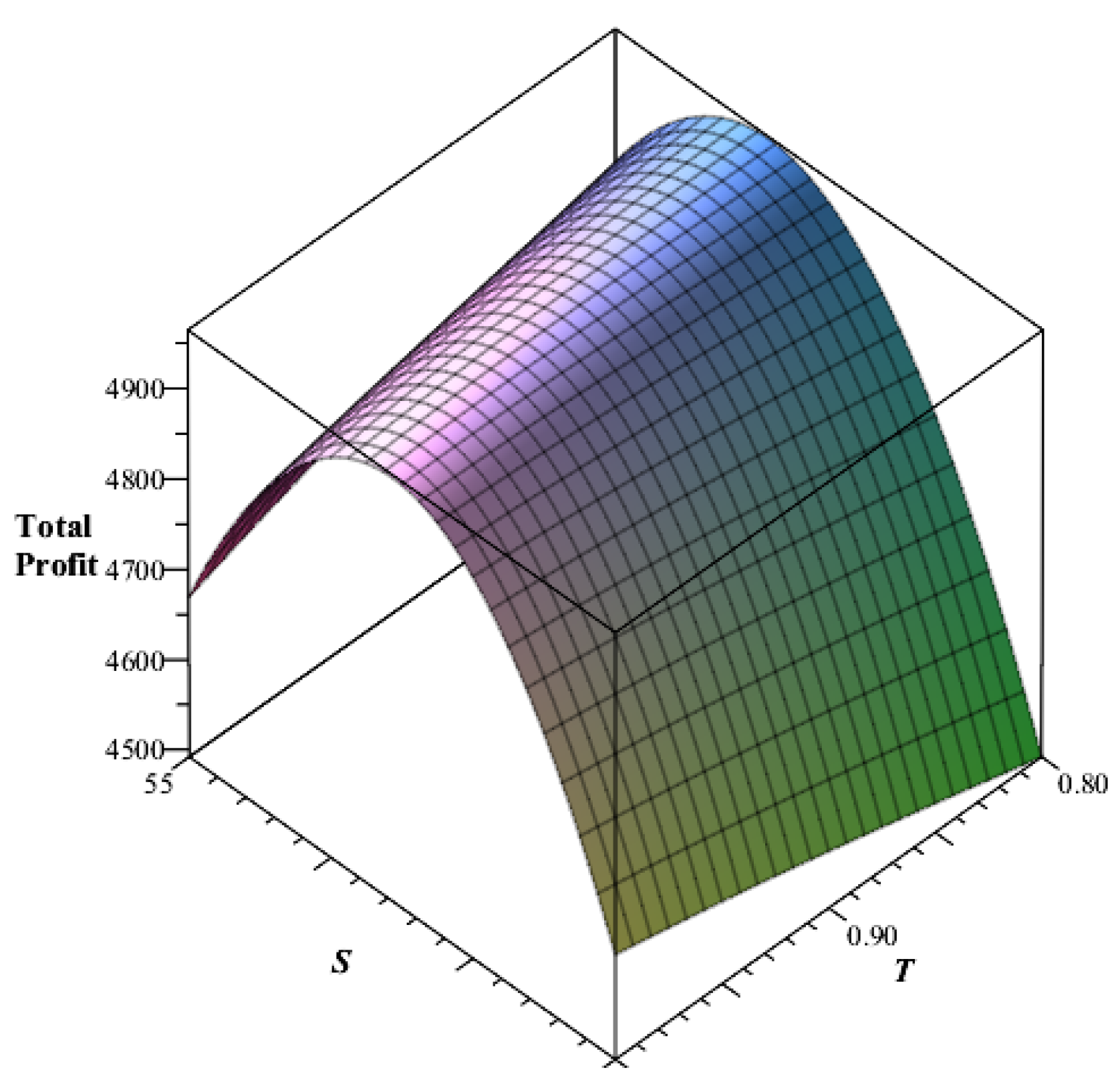
6.1. Numerical Illustrations

For determining this resultant model, this article reviewed three numerical illustrations, which facilitated in defining an optimal result for the profit function of the retailer. Additionally, for each case, the optimality of a total profit function is shown by the graphs.

Illustration 1: For situation-(i): $0<M<t_n<T$

For an inventory system, consider the following measures:

$a=1000$, $b=11$, $P=\$30$/unit, $\omega =0.005$, $P_d=\$50$/unit, $\tau =0.4$, $\psi =0.35$, $D_0=5$, $M=0.3$ years, $h=\$0.2$/unit/year, $O=\$50$/order, ${\theta }_n=0.2$, $I_g=0.1$/dollar/year, $I_p=0.12$/dollar/year, $\varphi =0.2$. Now, by using the above phrases, the decision variable’s optimal measures are $T^{*}=1.580$ years, and $S^{*}=\$68.72$. Thus, the optimal time when there is no deterioration is $t_n{}^{*}=\varphi T^{*}=0.316$ and the optimal order quantity is $Q^{*}=302.10$ with total profit $T{P}_1\left(S^{*},T^{*}\right)=\$3736.77$. The Hessian matrix for this situation is $H_1\left(S^{*},T^{*}\right)=\left[\begin{array}{cc}-14.52& 82.42\\ 82.42& -2600.35\end{array}\right]$ with principal minor determinants $D_1=\left|\frac{{\partial }^{2}T{P}_i\left(S^{*},T^{*}\right)}{\partial S^2}\right|=-14.52<0, D_2=\left|\begin{array}{cc}\frac{{\partial }^{2}T{P}_i\left(S^{*},T^{*}\right)}{\partial S^2}& \frac{{\partial }^{2}T{P}_i\left(S^{*},T^{*}\right)}{\partial S\partial T}\\ \frac{{\partial }^{2}T{P}_i\left(S^{*},T^{*}\right)}{\partial T\partial S}& \frac{{\partial }^{2}T{P}_i\left(S^{*},T^{*}\right)}{\partial T^2}\end{array}\right|=\mathrm{30,964.02}>0$. Additionally, the sufficient conditions of the second-order partial derivatives are

$$\begin{array}{l}\left|\begin{array}{cc}-14.52& 82.42\\ 82.42& -2600.35\end{array}\right|=\mathrm{30,964.02}>0\hspace{1em}\mathrm{and}\\ \frac{{\partial }^{2}T{P}_i\left(S^{*},T^{*}\right)}{\partial S^2}=-14.52<0,\hspace{1em}\frac{{\partial }^{2}T{P}_i\left(S^{*},T^{*}\right)}{\partial T^2}=-2600.35<0\end{array}$$

Hence, it is observed that all the principal minor determinants have alternative signs, whereas the even principal minors have positive signs. Therefore, from Proposition 1, the Hessian matrix $H_1\left(S^{*},T^{*}\right)$ is negative definite; from Proposition 2, a stationary point $\left(S^{*},T^{*}\right)$ is maximum; and from Proposition 3, the total profit function $T{P}_1\left(S^{*},T^{*}\right)$ is a strictly concave function and attains a maximum value at the optimal measure $\left(S^{*},T^{*}\right)$, and its graphical representation is also shown in Figure 2.

Figure 2. Optimality of a total profit function for situation 1 ($0<M<t_n<T$).

Illustration 2: For situation-(ii): $0<t_n<M<T$

Considering the same data as per example 1 except $M=0.4$ years and by using the above phrases, the decision variables’ optimal measures are $T^{*}=1.589$ years, and $S^{*}=\$68.55$. Thus, the optimal time when there is no deterioration is $t_n{}^{*}=\phi T^{*}=0.317$ and the optimal order quantity is $Q^{*}=307.78$ with total profit $T{P}_2\left(T^{*},S^{*}\right)=\$3814.73$. The Hessian matrix for this situation is $H_2\left(S^{*},T^{*}\right)=\left[\begin{array}{cc}-14.60& 82.78\\ 82.78& -2609.12\end{array}\right]$ with principal minor determinants

$$D_1=\left|\frac{{\partial }^{2}T{P}_i\left(S^{*},T^{*}\right)}{\partial S^2}\right|=-14.60<0, D_2=\left|\begin{array}{cc}\frac{{\partial }^{2}T{P}_i\left(S^{*},T^{*}\right)}{\partial S^2}& \frac{{\partial }^{2}T{P}_i\left(S^{*},T^{*}\right)}{\partial S\partial T}\\ \frac{{\partial }^{2}T{P}_i\left(S^{*},T^{*}\right)}{\partial T\partial S}& \frac{{\partial }^{2}T{P}_i\left(S^{*},T^{*}\right)}{\partial T^2}\end{array}\right|=\mathrm{31,240.62}>0$$

Additionally, the sufficient conditions of the second-order partial derivatives are

$$\begin{array}{l}\left|\begin{array}{cc}-14.60& 82.78\\ 82.78& -2609.12\end{array}\right|=\mathrm{31,240.62}>0\hspace{1em}\mathrm{and}\\ \frac{{\partial }^{2}T{P}_i\left(S^{*},T^{*}\right)}{\partial S^2}=-14.60<0,\hspace{1em}\frac{{\partial }^{2}T{P}_i\left(S^{*},T^{*}\right)}{\partial T^2}=-2609.12<0\end{array}$$

Hence, it is observed that all the principal minor determinants have alternative signs, whereas the even principal minors have positive signs. Therefore, from Proposition 1, the Hessian matrix $H_2\left(S^{*},T^{*}\right)$ is negative definite; from Proposition 2, a stationary point $\left(S^{*},T^{*}\right)$ is maximum; and from Proposition 3, the total profit function $T{P}_2\left(S^{*},T^{*}\right)$ is a strictly concave function and attains a maximum value at the optimum measure $\left(S^{*},T^{*}\right)$, and its graphical representation is also shown in Figure 3.

Figure 3. Optimality of a total profit function for situation 2 ($0<t_n<M<T$).

Illustration 3: For situation-(iii): $0<t_n<T<M$

Considering the same data as per example 1, except $M=1.3$ years, and by using the above phrases, the decision variables’ optimal measures are $T^{*}=0.918$ years, and $S^{*}=\$61.44$. Thus, the optimal time when there is no deterioration is $t_n{}^{*}=\varphi T^{*}=0.184$ and the optimal order quantity is $Q^{*}=138.15$ with total profit $T{P}_3\left(S^{*},T^{*}\right)=\$4964.62$. The Hessian matrix for this situation is $H_3\left(S^{*},T^{*}\right)=\left[\begin{array}{cc}-10.91& 95.51\\ 95.51& -1587.93\end{array}\right]$ with principal minor determinants

$$D_1=\left|\frac{{\partial }^{2}T{P}_i\left(S^{*},T^{*}\right)}{\partial S^2}\right|=-10.91<0, D_2=\left|\begin{array}{cc}\frac{{\partial }^{2}T{P}_i\left(S^{*},T^{*}\right)}{\partial S^2}& \frac{{\partial }^{2}T{P}_i\left(S^{*},T^{*}\right)}{\partial S\partial T}\\ \frac{{\partial }^{2}T{P}_i\left(S^{*},T^{*}\right)}{\partial T\partial S}& \frac{{\partial }^{2}T{P}_i\left(S^{*},T^{*}\right)}{\partial T^2}\end{array}\right|=8202.16>0$$

Additionally, the sufficient conditions of the second-order partial derivatives are

$$\begin{array}{l}\left|\begin{array}{cc}-10.91& 95.51\\ 95.51& -1587.93\end{array}\right|=8202.16>0\hspace{1em}\mathrm{and}\\ \frac{{\partial }^{2}T{P}_i\left(S^{*},T^{*}\right)}{\partial S^2}=-10.91<0, \frac{{\partial }^{2}T{P}_i\left(S^{*},T^{*}\right)}{\partial T^2}=-1587.93<0\end{array}$$

Hence, it is observed that all the principal minor determinants have alternative signs, whereas the even principal minors have positive signs. Therefore, from Proposition 1, the Hessian matrix $H_3\left(S^{*},T^{*}\right)$ is negative definite; from Proposition 2, a stationary point $\left(S^{*},T^{*}\right)$ is maximal; and from Proposition 3, the total profit function $T{P}_3\left(S^{*},T^{*}\right)$ is a strictly concave function and attains a maximum value at the optimum measure $\left(S^{*},T^{*}\right)$, and its graphical representation is also shown in Figure 4.

Figure 4. Optimality of a total profit function for situation 3 ($0<t_n<T<M$).

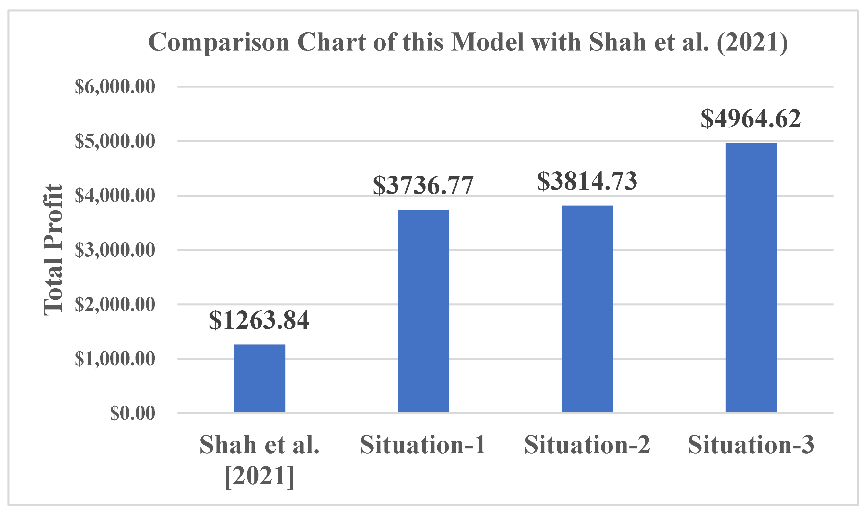
6.2. Comparison Chart

The model [28] develops a dynamic pricing policy for non-instantaneous deteriorating items with time-varying holding costs, where the nature of the sales price is considered to be constant and time dependent. This research is now being expanded [28] by taking into account the retailer and supplier’s trade credit policy. The retailer may face three distinct situations as a result of this policy, as defined and expressed in Table 2. This section displays a comparison chart of the retailer’s total profit between the previous model [28] and the current model, as shown in Figure 5.

Figure 5. Comparison chart of current model with [28].

From Figure 5, it is observed that the retailer will generate more profit if the retailer receives the credit period from the supplier. In addition, the various situations indicate that as the credit period increases, the total profit of the retailer also increases. Therefore, if the retailer receives a higher credit period from the supplier, then the retailer generates the maximum revenue. As a result, the inclusion of a trade credit policy benefits both the supplier and retailer by increasing the demand for goods and generating revenue by earning some interest.

6.3. Sensitivity Analysis

In Example 2, the sensitivity analysis is accomplished in this section, for the various inventory parameters, by adjusting one parameter at a time as −20%, −10%, 10%, and 20%, and the results are revealed in Table 3, Table 4, Table 5, Table 6, Table 7, Table 8, Table 9, Table 10, Table 11, Table 12 and Table 13 below.

Table 3. Impact of market potential $\left(a\right)$.

$\mathit{a}$	$\mathit{T}$	$\mathit{S}$	$\mathit{Q}$	$\mathit{T}{\mathit{P}}_2\left(\mathit{S},\mathit{T}\right)$
800	1.211	57.38	126.13	1473.63
900	1.404	62.97	204.82	2476.34
1100	1.765	74.11	436.25	5524.50
1200	1.855	77.87	580.36	6728.10

Table 4. Impact of price sensitivity factor $\left(b\right)$.

$\mathit{b}$	$\mathit{T}$	$\mathit{S}$	$\mathit{Q}$	$\mathit{T}{\mathit{P}}_2\left(\mathit{S},\mathit{T}\right)$
8.8	1.989	81.65	529.05	6898.85
9.9	1.784	74.75	407.15	5174.67
12.1	1.421	63.45	234.11	2835.47
13.2	1.275	59.18	178.89	2117.52

Table 5. Impact of purchasing cost $\left(P\right)$.

$\mathit{P}$	$\mathit{T}$	$\mathit{S}$	$\mathit{Q}$	$\mathit{T}{\mathit{P}}_2\left(\mathit{S},\mathit{T}\right)$
24	1.847	66.15	456.39	5238.21
27	1.714	67.36	375.28	4480.38
33	1.472	69.73	251.62	3231.24
36	1.363	70.89	204.90	2721.35

Table 6. Impact of holding cost $\left(h\right)$.

$\mathit{h}$	$\mathit{T}$	$\mathit{S}$	$\mathit{Q}$	$\mathit{T}{\mathit{P}}_2\left(\mathit{S},\mathit{T}\right)$
0.16	1.593	68.55	309.11	3822.37
0.18	1.591	68.55	308.46	3818.66
0.22	1.587	68.55	307.09	3811.19
0.24	1.586	68.56	306.42	3807.33

Table 7. Impact of ordering cost $\left(O\right)$.

$\mathit{O}$	$\mathit{T}$	$\mathit{S}$	$\mathit{Q}$	$\mathit{T}{\mathit{P}}_2\left(\mathit{S},\mathit{T}\right)$
40	1.587	68.54	307.21	3820.99
45	1.588	68.55	307.51	3818.02
55	1.590	68.56	308.60	3811.55
60	1.591	68.56	308.64	3808.65

Table 8. Impact of deterioration rate $\left({\theta }_n\right)$.

${\mathit{\theta }}_{\mathit{n}}$	$\mathit{T}$	$\mathit{S}$	$\mathit{Q}$	$\mathit{T}{\mathit{P}}_2\left(\mathit{S},\mathit{T}\right)$
0.16	1.845	68.37	401.13	4350.09
0.18	1.708	68.46	349.83	4065.43
0.22	1.486	68.63	272.76	3594.14
0.24	1.395	68.70	243.43	3397.45

Table 9. Impact of the reduced rate of sales $\left(\psi \right)$.

$\mathit{\psi }$	$\mathit{T}$	$\mathit{S}$	$\mathit{Q}$	$\mathit{T}{\mathit{P}}_2\left(\mathit{S},\mathit{T}\right)$
0.28	1.611	68.74	325.11	3931.83
0.31	1.599	68.63	315.02	3864.32
0.38	1.580	68.48	300.78	3766.63
0.42	1.568	68.38	291.79	3704.49

Table 10. Impact of initial rate of demand $\left(D_0\right)$.

${\mathit{D}}_0$	$\mathit{T}$	$\mathit{S}$	$\mathit{Q}$	$\mathit{T}{\mathit{P}}_2\left(\mathit{S},\mathit{T}\right)$
4	1.591	68.51	307.76	3793.32
4.5	1.590	68.53	307.78	3803.52
5.5	1.588	68.57	307.80	3826.31
6	1.587	68.59	307.81	3837.27

Table 11. Impact of upstream trade credit $\left(M\right)$.

$\mathit{M}$	$\mathit{T}$	$\mathit{S}$	$\mathit{Q}$	$\mathit{T}{\mathit{P}}_2\left(\mathit{S},\mathit{T}\right)$
0.24	1.574	68.82	298.42	3692.01
0.27	1.577	68.77	300.24	3714.38
0.33	1.589	68.72	308.51	3792.03
0.36	1.592	68.67	310.28	3815.69

Table 12. Impact of interest gain $\left(I_g\right)$.

${\mathit{I}}_{\mathit{g}}$	$\mathit{T}$	$\mathit{S}$	$\mathit{Q}$	$\mathit{T}{\mathit{P}}_2\left(\mathit{S},\mathit{T}\right)$
0.08	1.591	68.57	308.16	3810.23
0.09	1.590	68.56	307.96	3812.64
0.11	1.588	68.54	307.57	3817.19
0.12	1.587	68.53	307.38	3819.59

Table 13. Impact of interest paid $\left(I_p\right)$.

${\mathit{I}}_{\mathit{p}}$	$\mathit{T}$	$\mathit{S}$	$\mathit{Q}$	$\mathit{T}{\mathit{P}}_2\left(\mathit{S},\mathit{T}\right)$
0.096	1.643	68.59	327.74	3902.40
0.108	1.615	68.57	317.46	3857.67
0.132	1.564	68.53	298.57	3773.95
0.144	1.540	68.51	289.87	3734.09

Impact of Scale Demand (a): The parameter (a) can be considered as the maximum demand that a company can assess in a particular cycle time. The cycle time $\left(T\right)$, sales price $\left(S\right)$, order quantity $\left(Q\right)$, and overall profit $T{P}_2\left(S,T\right)$ all increase as the scale demand rate rises. Thus, the increase is favorable to this model since it increases the retailer’s net profit.

Impact of Price Sensitivity Factor (b): The parameter $\left(b\right)$ indicates that the product’s sale decreases as its sales price increases. The $\left(Q\right)$, $\left(T\right)$, $\left(S\right)$, and $T{P}_2\left(S,T\right)$ all decrease as the $\left(b\right)$ increases. The increase has a negative impact since it reduces the overall profit function.

Impact of Purchasing Cost $\left(P\right)$: The sales price $\left(S\right)$ increases as the cost price $\left(P\right)$ increases, while the cycle time $\left(T\right)$, order quantity $\left(Q\right)$, and overall profit $T{P}_2\left(S,T\right)$ decrease. The impact of purchasing cost $\left(P\right)$ on sales price $\left(S\right)$ and overall profit $T{P}_2\left(S,T\right)$ is quite significant. As a result, the increase is unfavorable.

Impact of parameter Holding Cost $\left(h\right)$: As the parameter $\left(h\right)$ rises, $\left(Q\right)$, $\left(T\right)$, and overall profit $T{P}_2\left(S,T\right)$ decreases, which suggests that the increase is unfavorable to this model.

Impact of Ordering Cost $\left(O\right)$: The sales price $\left(S\right)$, $\left(T\right)$, and $\left(Q\right)$ increases as the ordering cost $\left(O\right)$ surges, while overall profit $T{P}_2\left(S,T\right)$ decreases. Thus, an increase in ordering cost decreases the retailer’s overall profit, which suggests that the increase is not favorable to this model.

Impact of Deterioration Rate $\left({\theta }_n\right)$: The sales price $\left(S\right)$ increases as $\left({\theta }_n\right)$ increases while the $\left(T\right)$, $\left(Q\right)$, and the overall profit $T{P}_2\left(S,T\right)$ decrease. Thus, there is a negative impact of the deterioration on the retailer’s overall profit. The results are reliable to the result of [8,10], who discovered that as the deterioration increases, the total profit per unit of time decreases.

Impact of The Reduced Rate of Sales $\left(\psi \right)$:$\left(\psi \right)$ represents the saturation impact. The cycle time $\left(T\right)$, sales price $\left(S\right)$, order quantity $\left(Q\right)$, and overall profit $T{P}_2\left(S,T\right)$ decrease as $\left(\psi \right)$ increases. The change has a negative impact since it decreases sales price, which affects the net profit function. The net profit function decreases as the saturation impact increases. The result follows the study by [28], who observe that the total profit function decreases with an increase in saturation effect.

Impact of Initial Rate of Demand $\left(D_0\right)$: Cycle time $\left(T\right)$ diminutions as the initial rate of demand $\left(D_0\right)$ rise while sales price $\left(S\right)$, order quantity $\left(Q\right)$, and overall profit $T{P}_2\left(S,T\right)$ increase. The increase is beneficial for the retailer since it increases the total profit.

Impact of Upstream Trade Credit $\left(M\right)$: The cycle time $\left(T\right)$, sales price $\left(S\right)$, order quantity $\left(Q\right)$, and overall profit $T{P}_2\left(S,T\right)$ increase as the credit period $\left(M\right)$ increases while sales price $\left(S\right)$ decreases, which implies that when the credit time $\left(M\right)$ is longer, the overall profit of the retailer would be larger as well. A similar result is observed in [3,18].

Impact of Interest Gain $\left(I_g\right)$: The cycle time $\left(T\right)$, sales price $\left(S\right)$, and order quantity $\left(Q\right)$ decrease as interest gain $\left(I_g\right)$ increases, while overall profit $T{P}_2\left(S,T\right)$ increases. Hence, the increase is favorable to this model.

Impact of Interest Paid $\left(I_p\right)$: The cycle time $\left(T\right)$, sales price $\left(S\right)$, order quantity $\left(Q\right)$, and overall profit $T{P}_2\left(S,T\right)$ decrease as interest paid $\left(I_p\right)$ increases. Thus, the increase $\left(I_p\right)$ is not desirable as the overall profit function declines.

6.4. Managerial Implications

The following results are derived from the aforementioned insights, which may assist the retailer/decision-maker in making the proper decision for the optimal business policy, and by the analyses of this model, the retailer should consider all of these below aspects so that management may utilize this idea for business purposes to maximize profit:

• It is observed that the overall profit for the retailer under the proposed model is maximal when the initial rate of demand of a customer and the scaling demand of a product is high, which proposes to the retailer that if the initial customer’s demand for a product is high, then it would be better for the retailer to order a large number of units.
• The price-sensitive parameter and reduced rate of sales parameter affect negatively a retailer’s total profit as they decrease the sales price of a product. Therefore, the increase is not beneficial for the retailer.
• The increase in the purchasing cost of a unit rises the sales price, and it is noticeable that an increase in the sales price would have a direct impact on the demand rate. Thus, the total profit will decrease as demand decreases. Therefore, if the purchasing cost of a product is high, then the retailer should not place any order.
• The increase in holding cost and ordering cost of a product is not beneficial for the retailer, as it decreases the overall profit for a retailer. Hence, if the ordering cost and holding cost both are low, then the retailer should order more units so that the retailer can easily carry the inventory to achieve the maximum profit when the demand for a product is high.
• When the rate of deterioration is high, the retailer does not need to hold items for an extended period. It is not recommended because the increase decreases total profit.
• Since the trade credit period and interest gain increase the retailer’s overall profit, it suggests that if the retailer obtains a higher credit period from a supplier, then the retailer should accept the proposal of a supplier and order more units to achieve maximum profit.

7. Conclusions

This work is beneficial where the demand is a key factor in increasing sales, and when a business is facing problems due to spoilage, this article helps to solve the situation. They can have variations with appropriate discounts for perishable items during the deteriorating time instead of a constant sales price. In inventory management, dynamic pricing is an effective technique, and this will support them to satisfy customers’ requirements according to their demands. In particular, when customer demand is price sensitive, a business might adjust its price over time. When deterioration occurs, the model analyzes dynamic pricing strategies for perishable items, where the sales price is time dependent and is a function of the exponential with the discount variable. This study extends the model of [28] by incorporating a trade credit policy between the supplier and the retailer. The results are also compared to model [28], which shows the higher retailer’s total profit in various situations. Moreover, according to the results of this study, if any industry wants to implement a new policy to increase profits, a higher credit period is the best option. The algorithm rule is developed for the optimality of the retailer’s overall profit function. To determine the cycle time and initial sales price, this study includes the traditional optimization approach. Finally, to examine the implementation of significant parameters, a sensitivity analysis is achieved for the overall profit of the retailer. Therefore, by assimilating the above results and from the sensitivity table, it is advised that the business sell as many items as possible before deterioration occurs, and the higher credit period will be the best technique for the retailer to achieve the maximum overall profit. Increases in holding costs, ordering costs, and purchasing costs have a negative impact on the total profit function, so retailers should try to minimize these costs to maximize revenue.

Existing research can be further stretched by considering shortages and preservation technology investment as considered in the work of [18], multi-item integrated supply chain as suggested in the work of [30], two-stage trade credit financing [4], diverse demand types for example advertisement dependent [10] and stochastic dependent [13].

References

- Goyal, S.K. Economic ordering policy for deteriorating items over an infinite time horizon. Eur. J. Oper. Res. 1987, 28, 298–301. [Google Scholar] [CrossRef]
- Sarkar, B. An EOQ model with delay in payments and stock-dependent demand in the presence of imperfect production. Appl. Math. Comput. 2012, 218, 8295–8308. [Google Scholar] [CrossRef]
- Liu, G.; Zhang, J.; Tang, W. Joint dynamic pricing and investment strategy for perishable food with price-quality dependent demand. Ann. Oper. Res. 2015, 216, 397–416. [Google Scholar] [CrossRef]
- Dye, C.-Y.; Yang, C.-T. Optimal dynamic pricing and preservation technology investment for deteriorating products with reference price effects. Omega 2016, 62, 52–67. [Google Scholar] [CrossRef]
- Ghoreishi, M.; Weber, G.W.; Mirzazadeh, A. An inventory model for non-instantaneous deteriorating items with partial backlogging, permissible delay in payments, inflation, and selling price-dependent demand and customer returns. Ann. Oper. Res. 2018, 226, 221–238. [Google Scholar] [CrossRef]
- Tayal, S.; Singh, S.R.; Sharma, R.; Singh, A.P. An EPQ model for non-instantaneous deteriorating items with time-dependent holding cost and exponential demand rate. Int. J. Oper. Res. 2015, 23, 145–162. [Google Scholar] [CrossRef]
- Ai, X.Y.; Zhang, J.L.; Wang, L. Optimal joint replenishment policy for multiple non-instantaneous deteriorating items. Int. J. Prod. Res. 2017, 55, 4625–4642. [Google Scholar] [CrossRef]
- Tiwari, S.; Ahmed, W.; Sarkar, B. Sustainable ordering policies for non-instantaneous deteriorating items under carbon emission and multi-trade-credit-policies. J. Clean. Prod. 2019, 240, 118183. [Google Scholar] [CrossRef]
- Li, G.; He, X.; Zhou, J.; Wu, H. Pricing replenishment and preservation technology investment decisions for non-instantaneous deterioration items. Omega 2019, 84, 114–126. [Google Scholar] [CrossRef]
- Udayakumar, R.; Geetha, K.V.; Sana, S.S. Economic ordering policy for non-instantaneous deteriorating items with price and advertisement dependent demand and permissible delay in payment under inflation. Math. Methods Appl. Sci. 2021, 44, 7697–7721. [Google Scholar] [CrossRef]
- Zhao, W.; Zheng, Y.S. Optimal dynamic pricing for perishable assets with nonhomogeneous demand. Manag. Sci. 2000, 46, 375–388. [Google Scholar] [CrossRef]
- Dasu, S.; Tong, C. Dynamic pricing when consumers are strategic: Analysis of posted and contingent pricing schemes. Eur. J. Oper. Res. 2010, 204, 662–671. [Google Scholar] [CrossRef]
- Taleizadeh, A.A.; Niaki, S.T.A.; Seyedjavadi, S.M.H. Multi-product multi-chance-constraint stochastic inventory control problem with dynamic demand and partial back-ordering: A harmony search algorithm. J. Manuf. Syst. 2012, 31, 204–213. [Google Scholar] [CrossRef]
- Tan, B.; Karabati, S. Retail inventory management with stock-out-based dynamic demand substitution. Int. J. Prod. Econ. 2013, 145, 78–87. [Google Scholar] [CrossRef] [Green Version]
- Hu, X.; Wan, Z.; Murthy, N.N. Dynamic pricing of limited inventories with product returns. Manuf. Serv. Oper. Manag. 2019, 21, 501–518. [Google Scholar] [CrossRef]
- ABC News. Amazon Error May End “Dynamic Pricing”. 2000. Available online: http://abcnews.go.com/Technology/story?id=119399 (accessed on 20 May 2020).
- Saren, S.; Sarkar, B.; Bachar, R.K. Application of various price-discount policies for deteriorated products and delay in payments in an advanced inventory model. Inventions 2020, 5, 50. [Google Scholar] [CrossRef]
- Lin, M.; Sengupta, I. Analysis of Optimal Portfolio on Finite and Small-Time Horizons for a Stochastic Volatility Market Model. SIAM J. Financ. Math. 2021, 12, 1596–1624. [Google Scholar] [CrossRef]
- Ding, Y.; Jiang, Y.; Wu, L.; Zhou, Z. Two-echelon supply chain network design with trade credit. Comput. Oper. Res. 2021, 131, 105270. [Google Scholar] [CrossRef]
- Wu, K.S.; Ouyang, L.Y.; Yang, C.T. An optimal replenishment policy for non-instantaneous deteriorating items with stock dependent demand and partial backlogging. Int. J. Prod. Econ. 2006, 101, 369–384. [Google Scholar] [CrossRef]
- Bakker, M.; Riezebos, J.; Teunter, R.H. Review of inventory systems with a deterioration since 2001. Eur. J. Oper. Res. 2012, 221, 275–284. [Google Scholar] [CrossRef]
- Perez, F.; Torres, F. An integrated production-inventory model for deteriorating items to evaluate JIT purchasing alliances. Int. J. Ind. Eng. Comput. 2019, 10, 51–66. [Google Scholar] [CrossRef]
- Xu, W.; Zhao, K.; Shi, Y.; Bingzhen, S. The optimal pricing model for non-instantaneous deterioration items with price and freshness sensitive demand under the e-commerce environment in China. Kybernetes 2021, 51, 623–640. [Google Scholar] [CrossRef]
- Xue, M.; Tang, W.; Zhang, J. Optimal dynamic pricing for deteriorating items with reference price effects. Int. J. Syst. Sci. 2016, 47, 2022–2031. [Google Scholar] [CrossRef]
- Li, S.; Zhang, J.; Tang, W. Joint dynamic pricing and inventory control policy for a stochastic inventory system with perishable products. Int. J. Prod. Res. 2014, 53, 2937–2950. [Google Scholar] [CrossRef]
- Kumar, R.; Nasralah, H. Asymptotic Approximation of Optimal Portfolio for Small Time Horizons. SIAM J. Financ. Math. 2018, 9, 755–774. [Google Scholar] [CrossRef] [Green Version]
- Pathak, U.; Kant, R.; Shankar, R. Price and profit decisions in manufacturer-led dual-channel supply chain configurations. Int. J. Ind. Eng. Comput. 2020, 11, 377–400. [Google Scholar] [CrossRef]
- Shah, N.H.; Rabari, K.; Patel, E. Dynamic demand and pricing inventory model for non-instantaneous deteriorating items. Int. J. Math. Eng. Manag. Sci. 2021, 6, 510–521. [Google Scholar] [CrossRef]
- Pourmohammad-Zia, N.; Karimi, B.; Rezaei, J. Dynamic pricing and inventory control policies in a food supply chain of growing and deteriorating items. Ann. Oper. Res. 2021, 1–40. [Google Scholar] [CrossRef]
- Chiu, Y.; Chiu, T.; Pai, F.; Wu, H. A producer-retailer incorporated a multi-item EPQ problem with delayed differentiation, the expedited rate for common parts, multi-delivery, and scrap. Int. J. Ind. Eng. Comput. 2021, 12, 427–440. [Google Scholar]
Publisher’s Note: MDPI stays neutral with regard to jurisdictional claims in published maps and institutional affiliations. |
© 2022 by the authors. Licensee MDPI, Basel, Switzerland. This article is an open access article distributed under the terms and conditions of the Creative Commons Attribution (CC BY) license (https://creativecommons.org/licenses/by/4.0/).