On a Nonlinear Initial—Boundary Value Problem with Venttsel Type Boundary Conditions Arizing in Homogenization of Complex Heat Transfer Problems

Abstract

We consider a non-standard nonlinear singularly perturbed 2D initial-boundary value problem with Venttsel type boundary conditions, arising in homogenization of radiative-conductive heat transfer problems. We establish existence, uniqueness and regularity of a weak solution v. We obtained estimates for the derivatives $D_{t}v$, $D_1^{2}v$, $D_2^{2}v$, $D_1{D}_{2}v$ with a qualified order in the small parameter $\epsilon$.

1. Introduction

When homogenizing a number of problems of complex heat transfer in periodic structures, new nonstandard boundary and initial—boundary value problems appear (see, for example, articles [1,2,3] and references therein). To justify the corresponding asymptotic approximations, it is necessary to study the solvability of these problems, the qualitative properties of solutions, and the dependence the norms of solutions on the small parameter $\epsilon$, which characterizes the dimensions of the periodicity cell.

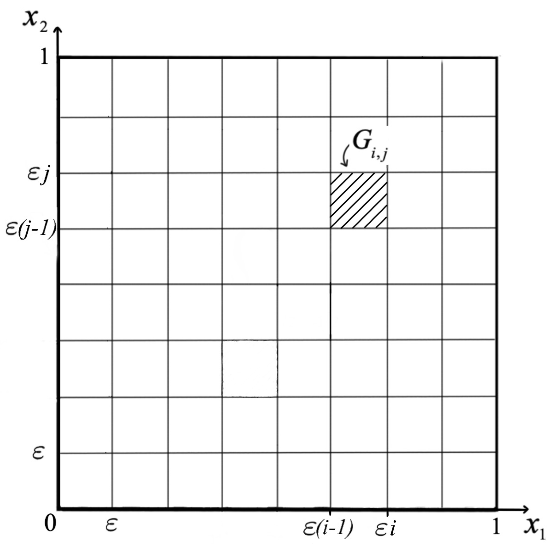
This article is devoted to the study of a nonstandard initial-boundary value problem

$$\begin{array}{cc}\hfill & c_p{D}_{t}v-\epsilon \Delta H\left(v\right)=f,(x,t)\in Q_{\epsilon ,T}={\Omega }_{\epsilon }\times (0,T),\hfill \end{array}$$

(1)

$$\begin{array}{cc}\hfill & {\displaystyle \frac{\epsilon }{2}}{c}_p{D}_{t}v+\epsilon D_{n}H\left(v\right)-\frac{{\epsilon }^2}{2}{D}_s^{2}H\left(v\right)+H_{\Gamma }\left(v\right)=g_{\Gamma }+{\displaystyle \frac{\epsilon }{2}}{f}_{\Gamma },(x,t)\in ({\Gamma }_{\epsilon }\setminus {\gamma }_{\epsilon })\times (0,T),\hfill \end{array}$$

(2)

$$\begin{array}{cc}\hfill & {\displaystyle \frac{\epsilon }{4}}{c}_p{D}_{t}v+\epsilon {\widehat{D}}_{n}H\left(v\right)+H_{\Gamma }\left(v\right)={\widehat{g}}_{\Gamma }+{\displaystyle \frac{\epsilon }{4}}{\widehat{f}}_{\Gamma },(x,t)\in {\gamma }_{\epsilon }\times (0,T),\hfill \end{array}$$

(3)

$$\begin{array}{cc}\hfill & {v|}_{t=0}=u^0,x\in {\Omega }_{\epsilon };v{{|}_{t=0}=v_{\Gamma }^0,x\in {\Gamma }_{\epsilon }\setminus {\gamma }_{\epsilon };v|}_{t=0}={\widehat{v}}_{\Gamma }^0,x\in {\gamma }_{\epsilon },\hfill \end{array}$$

(4)

which arises upon homogenization of the problem of radiative-conductive heat transfer (5)–(9). Here $0<\epsilon$ is a small parameter; $x=(x_1,x_2)$, ${\Omega }_{\epsilon }=I_{\epsilon }\times I_{\epsilon }$ (where $I_{\epsilon }=(\epsilon /2,1-\epsilon /2)$) is the square with boundary ${\Gamma }_{\epsilon }$, and ${\gamma }_{\epsilon }=\{A_{\epsilon },B_{\epsilon },C_{\epsilon },D_{\epsilon }\}$ is the set of its corner points (Figure 1).

Figure 1. The sets ${\Omega }_{\epsilon }$, ${\Gamma }_{\epsilon }$ and ${\gamma }_{\epsilon }$.

Everywhere below $D_t=\partial /\partial t$, $D_1=\partial /\partial x_1$, $D_2=\partial /\partial x_2$ and $D_n$, $D_s$ are the derivatives along the outward normal and tangent to ${\Gamma }_{\epsilon }$. At corner points

$$\begin{array}{cc}\hfill & {\widehat{D}}_n{|}_{x=A_{\epsilon }}=-\frac{1}{2}(D_1+D_2){|}_{x=A_{\epsilon }},{\widehat{D}}_n{{|}_{x=B_{\epsilon }}=\frac{1}{2}(-D_1+D_2)|}_{x=B_{\epsilon }},\hfill \\ \hfill & {\widehat{D}}_n{|}_{x=C_{\epsilon }}=\frac{1}{2}(D_1+D_2){|}_{x=C_{\epsilon }},{\widehat{D}}_n{{|}_{x=D_{\epsilon }}=\frac{1}{2}(D_1-D_2)|}_{x=D_{\epsilon }}.\hfill \end{array}$$

The problem (1)–(4) is singularly perturbed. Its solution depends on the small parameter $\epsilon$, but we omit $\epsilon$ in order to simlify the notation.

The boundary conditions (2) are non-linear conditions of the Venttsel type [4], since they include the time derivative and the second derivatives of the unknown function along the tangent direction. In addition, these conditions are supplemented by conditions (3) at corner points.

The study of parabolic initial-boundary value problems with Venttsel type conditions was started in [5,6,7,8,9,10]. References to later works can be found, for example, in [11,12,13].

The stationary analogue of the problem (1)–(4) was studied in [3].

Let’s give a brief description of the problem leading to (1)–(4). Consider the nonstationary radiative-conductive heat transfer problem in periodic system consisting of $n^2$ heat-conducting square-section rods separated by vacuum layers and placed in a square box $\Omega ={(0,1)}^2$ with boundary $\Gamma$ (Figure 2).

Figure 2. The sets $G_{ij}$ and $G={\displaystyle \bigcup _{1\le i\le n,1\le j\le n}}{G}_{ij}$.

With each rod we associate the elementary square

$$G_{ij}=((i-1)\epsilon ,i\epsilon )\times ((j-1)\epsilon ,j\epsilon ),1\le i\le n,1\le j\le n,$$

where $\epsilon =1/n$. The sought function $u(x,t)$ is interpreted as the absolute temperature at the point $x\in G={\displaystyle \bigcup _{1\le i\le n,1\le j\le n}}{G}_{ij}$ at time t and is defined on the set $G\times (0,T)$ (Figure 2).

The heat propogation inside G is decribed by the equation

$$c_p{D}_{t}u-div(\lambda \nabla u)=f,(x,t)\in G\times (0,T).$$

(5)

Here $0<c_p$ is the heat capacity coefficient, $0<\lambda$ is the thermal conductivity coefficient, f is the density of internal sources.

The heat exchange by radiation on the boundaries of neighboring rods is described by conditions

$$\begin{array}{cc}\hfill & \lambda D_{1}u(i\epsilon -0,x_2,t)=\lambda D_{1}u(i\epsilon +0,x_2,t))=\theta \left[h\left(u(i\epsilon +0,x_2,t)\right)-h\left(u(i\epsilon -0,x_2,t)\right)\right],\hfill \\ \hfill & x_2\in ((j-1)\epsilon ,j\epsilon ),0<i<n,1\le j\le n,t\in (0,T),\hfill \end{array}$$

(6)

$$\begin{array}{cc}\hfill \left[5pt\right]& \lambda D_{2}u(x_1,j\epsilon -0,t)=\lambda D_{2}u(x_1,j\epsilon +0,t)=\theta \left[h\left(u(x_1,j\epsilon +0,t)\right)-h\left(u(x_1,j\epsilon -0,t)\right)\right],\hfill \\ \hfill & x_1\in ((i-1)\epsilon ,i\epsilon ),1\le i\le n,0<j<n,t\in (0,T).\hfill \end{array}$$

(7)

Here $h\left(u\right)={\sigma }_0{\left|u\right|}^{3}u$, $0<{\sigma }_0$ is the Stefan—Boltzmann constant, $0<\theta \le 1$ is the apparent emmitance ($\theta =1$ for absolutely black rods).

Heat exchange by radiation with the boundary of the box having given temperature $u_{\Gamma }(x,t)$ is described by the boundary condition

$$\begin{array}{cc}\hfill & \lambda D_{n}u+{\theta }_{\Gamma }h\left(u\right)=w_{\Gamma },(x,t)\in \Gamma \times (0,T),\hfill \end{array}$$

(8)

where $w_{\Gamma }={\theta }_{\Gamma }h\left(u_{\Gamma }\right)$ and $0<{\theta }_{\Gamma }\le 1$ is the apparent emmitance.

Equation (5) and boundary conditions (6), (7) are supplemented by the initial condition

$$\begin{array}{cc}\hfill & {u|}_{t=0}=u^0,x\in G.\hfill \end{array}$$

(9)

The simplest homogenization of the problem (5)–(9), performed as in [3], leads to the problem (1)–(4), where

$$\begin{array}{c}\hfill H\left(v\right)=\theta h\left(v\right),H_{\Gamma }\left(u\right)={\theta }_{\Gamma }h\left(v\right).\end{array}$$

(10)

$$(f{|}_{{\Omega }_{\epsilon }}(x,t),f_{\Gamma }(x,t),{\widehat{f}}_{\Gamma }(x,t))={\Pi }_{\epsilon }f(x,t),(g_{\Gamma }(x,t),{\widehat{g}}_{\Gamma }(x,t))={\Pi }_{\epsilon }^{\Gamma }{w}_{\Gamma }(x,t),$$

and the operators ${\Pi }_{\epsilon }$, ${\Pi }_{\epsilon }^{\Gamma }$ are defined in Section 2.

The solution v to the problem (1)–(4) as $\epsilon \to 0$ is considered as an asymptotic approximation to the solution u to the problem (5)–(9). Problem (1)–(4), which approximates the problem (5)–(9), does not contain information on the value of the thermal conductivity coefficient $\lambda$. Computational experiments for the stationary problem [14] show that this is not essential for large values of $\lambda$. However it leads to the impossibility of practial usage of this approximation for small values of $\lambda$. A more accurate approximation, performed similarly to [3], taking into account the influence of the coefficient $\lambda$, leads to the problem (1)–(4) with

$$\begin{array}{c}\hfill H\left(v\right)=\underset{0}{\overset{v}{\int }}{\displaystyle \frac{h^{\prime }\left(t\right)dt}{{\displaystyle \frac{1}{\theta }}+{\displaystyle \frac{\epsilon }{\lambda }}{h}^{\prime }\left(t\right)}},H_{\Gamma }\left(v\right)=\underset{0}{\overset{v}{\int }}{\displaystyle \frac{h^{\prime }\left(t\right)dt}{{\displaystyle \frac{1}{{\theta }_{\Gamma }}}+{\displaystyle \frac{\epsilon }{2\lambda }}{h}^{\prime }\left(t\right)}}.\end{array}$$

(11)

and $w_{\Gamma }=H_{\Gamma }\left(u_{\Gamma }\right)$.

The paper is organized as follows. In Section 2 we introduce the used functional spaces and prove a number of auxiliary assertions. Section 3 contains results on the properties of the corresponding stationary problem, following from [3]. In Section 4 we define a weak solution to the problem (1)–(4) and prove upper and lower estimates for the weak solution. In Section 5, we prove the uniqueness of the weak solution. In Section 6, the existence of a weak solution is established and its estimates are derived. In Section 7 we establishe the result about regularity of the weak solution. Besides we derive estimates for the norms of the derivatives $D_{t}v$, $D_1^{2}v$, $D_1{D}_{2}v$, $D_2^{2}v$.

2. Some Notations and Function Spaces

Remind that ${\Omega }_{\epsilon }=I_{\epsilon }\times I_{\epsilon }$, where $I_{\epsilon }=(\epsilon /2,1-\epsilon /2)$, ${\Gamma }_{\epsilon }$ is a boundary of square ${\Omega }_{\epsilon }$ and ${\gamma }_{\epsilon }=\{A_{\epsilon },B_{\epsilon },C_{\epsilon },D_{\epsilon }\}$ is the set of its corner points. Note that

$$\begin{array}{cc}\hfill & {\Gamma }_{\epsilon }={\Gamma }_{\epsilon }^{\ell }\cup {\Gamma }_{\epsilon }^r\cup {\Gamma }_{\epsilon }^d\cup {\Gamma }_{\epsilon }^{up}\cup {\gamma }_{\epsilon },\hfill \end{array}$$

where

$$\begin{array}{cc}\hfill & {\Gamma }_{\epsilon }^{\ell }=\{\epsilon /2\}\times I_{\epsilon },{\Gamma }_{\epsilon }^r=\{1-\epsilon /2\}\times I_{\epsilon },{\Gamma }_{\epsilon }^d=I_{\epsilon }\times \{\epsilon /2\},{\Gamma }_{\epsilon }^{up}=I_{\epsilon }\times \{1-\epsilon /2\}.\hfill \end{array}$$

Also introduce the sets (Figure 3)

$$\begin{array}{cc}\hfill & {\Omega }_{\epsilon }^{\ell }=[0,\epsilon /2)\times I_{\epsilon },{\Omega }_{\epsilon }^r=(1-\epsilon /2,1]\times I_{\epsilon },{\Omega }_{\epsilon }^d=I_{\epsilon }\times [0,\epsilon /2),{\Omega }_{\epsilon }^{up}=I_{\epsilon }\times (1-\epsilon /2,1],\hfill \\ \hfill & {\Omega }_{\epsilon }^A=[0,\epsilon /2)\times [0,\epsilon /2),{\Omega }_{\epsilon }^B=[0,\epsilon /2)\times (1-\epsilon /2,1],{\Omega }_{\epsilon }^C=(1-\epsilon /2,1]\times (1-\epsilon /2,1],\hfill \\ \hfill & {\Omega }_{\epsilon }^D=(1-\epsilon /2,1]\times [0,\epsilon /2)\hfill \end{array}$$

and note that

$$\overline{\Omega }={\overline{\Omega }}_{\epsilon }\cup {\Omega }_{\epsilon }^{\ell }\cup {\Omega }_{\epsilon }^r\cup {\Omega }_{\epsilon }^d\cup {\Omega }_{\epsilon }^{up}\cup {\Omega }_{\epsilon }^A\cup {\Omega }_{\epsilon }^B\cup {\Omega }_{\epsilon }^C\cup {\Omega }_{\epsilon }^D.$$

Figure 3. The sets ${\Gamma }_{\epsilon }^{\ell }$, ${\Gamma }_{\epsilon }^r$, ${\Gamma }_{\epsilon }^d$, ${\Gamma }_{\epsilon }^{up}$ and ${\Omega }_{\epsilon }^{\ell }$, ${\Omega }_{\epsilon }^r$, ${\Omega }_{\epsilon }^d$, ${\Omega }_{\epsilon }^{up}$, ${\Omega }_{\epsilon }^A$, ${\Omega }_{\epsilon }^B$, ${\Omega }_{\epsilon }^C$, ${\Omega }_{\epsilon }^D$.

2.1. Spaces ${\mathcal{L}}_{\epsilon }^2$ and $L_{\epsilon }^2(\Omega )$

We introduce the Euclidean space $L^2\left({\gamma }_{\epsilon }\right)$ of functions h defined on ${\gamma }_{\epsilon }$ with the inner product and the norm respectively

$${(h_1,h_2)}_{L^2\left({\gamma }_{\epsilon }\right)}=\sum _{x\in {\gamma }_{\epsilon }}{h}_1\left(x\right)h_2\left(x\right),{\parallel h\parallel }_{L^2\left({\gamma }_{\epsilon }\right)}=\sqrt{{(h,h)}_{\epsilon }}.$$

We introduce the Hilbert space ${\mathcal{L}}_{\epsilon }^2=L^2\left({\Omega }_{\epsilon }\right)\times L^2\left({\Gamma }_{\epsilon }\right)\times L^2\left({\gamma }_{\epsilon }\right)$ with elements $y=(f,g,h)$, the inner product and the norm respectively

$${(y_1,y_2)}_{{\mathcal{L}}_{\epsilon }^2}={(f_1,f_2)}_{L^2\left({\Omega }_{\epsilon }\right)}+{\displaystyle \frac{\epsilon }{2}}{(g_1,g_2)}_{L^2\left({\Gamma }_{\epsilon }\right)}+{\displaystyle \frac{{\epsilon }^2}{4}}{(h_1,h_2)}_{L^2\left({\gamma }_{\epsilon }\right)},{\parallel y\parallel }_{{\mathcal{L}}_{\epsilon }}={(y,y)}_{{\mathcal{L}}_{\epsilon }}^{1/2}.$$

We define the operator ${\Pi }_{\epsilon }:L^2(\Omega )\to {\mathcal{L}}_{\epsilon }^2$ by the formula ${\Pi }_{\epsilon }f=\left({f|}_{{\Omega }_{\epsilon }},f_{\Gamma },{\widehat{f}}_{\Gamma }\right)\in {\mathcal{L}}_{\epsilon }^2$, where ${f|}_{{\Omega }_{\epsilon }}$ is the restriction of f to ${\Omega }_{\epsilon }$,

$$\begin{array}{cc}\hfill & f_{\Gamma }\left(x\right)=\left\{\begin{array}{cc}{\displaystyle {\displaystyle \frac{2}{\epsilon }}\underset{0}{\overset{\epsilon /2}{\int }}f(s,x_2)ds,}\hfill & x\in {\Gamma }_{\epsilon }^{\ell },\hfill \\ {\displaystyle {\displaystyle \frac{2}{\epsilon }}\underset{1-\epsilon /2}{\overset{1}{\int }}f(s,x_2)ds,}\hfill & x\in {\Gamma }_{\epsilon }^r,\hfill \\ {\displaystyle {\displaystyle \frac{2}{\epsilon }}\underset{0}{\overset{\epsilon /2}{\int }}f(x_1,s)ds,}\hfill & x\in {\Gamma }_{\epsilon }^d,\hfill \\ {\displaystyle {\displaystyle \frac{2}{\epsilon }}\underset{1-\epsilon /2}{\overset{1}{\int }}f(x_1,s)ds,}\hfill & x\in {\Gamma }_{\epsilon }^{up},\hfill \end{array}\right.\hfill \end{array}$$

(12)

$$\begin{array}{cc}& {\widehat{f}}_{\Gamma }\left(X_{\epsilon }\right)=\frac{4}{{\epsilon }^2}{(f,1)}_{L^2\left({\Omega }_{\epsilon }^X\right)},X=A,B,C,D.\hfill \end{array}$$

(13)

We also define the operator $R_{\epsilon }:{\mathcal{L}}_{\epsilon }^2\to L^2(\Omega )$ by the formula

$$\begin{array}{cc}\hfill & R_{\epsilon }(f,g,h)\left(x\right)=\left\{\begin{array}{cc}f\left(x\right),\hfill & x\in {\Omega }_{\epsilon },\hfill \\ g(\epsilon /2,x_2),\hfill & x\in {\Omega }_{\epsilon }^{\ell },\hfill \\ g(1-\epsilon /2,x_2),\hfill & x\in {\Omega }_{\epsilon }^r,\hfill \\ g(x_1,\epsilon /2),\hfill & x\in {\Omega }_{\epsilon }^d,\hfill \\ g(x_1,1-\epsilon /2),\hfill & x\in {\Omega }_{\epsilon }^{up},\hfill \\ h\left(X_{\epsilon }\right),\hfill & x\in {\Omega }_{\epsilon }^X,X=A,B,C,D.\hfill \end{array}\right.\hfill \end{array}$$

Note that $L_{\epsilon }^2(\Omega )=Im{R}_{\epsilon }$ is a closed subspace of $L^2(\Omega )$. The operator $R_{\epsilon }$ performs an isomorphism between ${\mathcal{L}}_{\epsilon }^2$ and $L_{\epsilon }^2(\Omega )$, where ${\Pi }_{\epsilon }=R_{\epsilon }^{-1}$ and

$${\parallel f\parallel }_{L^2(\Omega )}={\parallel {\Pi }_{\epsilon }f\parallel }_{{\mathcal{L}}_{\epsilon }^2}\forall f\in L_{\epsilon }^2(\Omega ).$$

We also define the operator ${\Pi }_{\epsilon }^{\Gamma }$, which associates with the function $w_{\Gamma }\in L^2(\Gamma )$ the pair of functions $(g_{\Gamma },{\widehat{g}}_{\Gamma })\in L^2\left({\Gamma }_{\epsilon }\right)\times L^2\left({\gamma }_{\epsilon }\right)$, where

$$\begin{array}{cc}\hfill & g_{\Gamma }\left(x\right)=\left\{\begin{array}{cc}{w}_{\Gamma }(0,x_2),\hfill & x=(\epsilon /2,x_2)\in {\Gamma }_{\epsilon }^{\ell },\hfill \\ w_{\Gamma }(1,x_2),\hfill & x=(1-\epsilon /2,x_2)\in {\Gamma }_{\epsilon }^r,\hfill \\ w_{\Gamma }(x_1,0),\hfill & x=(x_1,\epsilon /2)\in {\Gamma }_{\epsilon }^d,\hfill \\ w_{\Gamma }(x_1,1),\hfill & x=(x_1,1-\epsilon /2)\in {\Gamma }_{\epsilon }^{up},\hfill \end{array}\right.\hfill \end{array}$$

(14)

and

$$\begin{array}{cc}\hfill & {\widehat{g}}_{\Gamma }\left(X^{\epsilon }\right)=\frac{1}{\epsilon }{(w_{\Gamma },1)}_{L^2(\Gamma \cap {\Omega }_{\epsilon }^X)},X=A,B,C,D.\hfill \end{array}$$

(15)

2.2. The Space $V_{\epsilon }$

Denote by $C_0^{\infty }\left({\Gamma }_{\epsilon }\right)$ the space of functions defined on ${\Gamma }_{\epsilon }$, infinitely differentiable on each side of ${\Gamma }_{\epsilon }$ and equal to zero in some neighborhood of the corner points set ${\gamma }_{\epsilon }$.

Let $u\in L^2\left({\Gamma }_{\epsilon }\right)$, $k=1,2$. The function $y\in L^2\left({\Gamma }_{\epsilon }\right)$, satisfying the identity

$${(y,\psi )}_{L^2\left({\Gamma }_{\epsilon }\right)}={(-1)}^k{(u,D_s^k\psi )}_{L^2\left({\Gamma }_{\epsilon }\right)}\forall \psi \in C_0^{\infty }\left({\Gamma }_{\epsilon }\right)$$

is called the weak order k derivative of the function u along the tangent to ${\Gamma }_{\epsilon }$ and is denoted by $D_s^{k}u$.

We denote by $W^{1,2}\left({\Gamma }_{\epsilon }\right)$ the space of functions $v\in C\left({\Gamma }_{\epsilon }\right)$, that possess the weak derivative $D_{s}v\in L^2\left({\Gamma }_{\epsilon }\right)$. Let $t{r}_{\epsilon }u$ denote the trace of the function $u\in W^{1,2}\left({\Omega }_{\epsilon }\right)$ on ${\Gamma }_{\epsilon }$ and $tru$ denote the trace of the function $u\in W^{1,2}(\Omega )$ on $\Gamma$.

We introduce the space

$$V_{\epsilon }=W^{1,2}({\Omega }_{\epsilon };{\Gamma }_{\epsilon })=\{u\in W^{1,2}\left({\Omega }_{\epsilon }\right)|t{r}_{\epsilon }u\in W^{1,2}\left({\Gamma }_{\epsilon }\right)\}$$

with the inner product and the norm respectively

$$\begin{array}{cc}\hfill {(u,v)}_{V_{\epsilon }}& =\epsilon {(\nabla u,\nabla v)}_{L^2\left({\Omega }_{\epsilon }\right)}+\frac{{\epsilon }^2}{2}{(D_{s}t{r}_{\epsilon }u,D_{s}t{r}_{\epsilon }v)}_{L^2\left({\Gamma }_{\epsilon }\right)}+{(t{r}_{\epsilon }u,t{r}_{\epsilon }v)}_{L^2\left({\Gamma }_{\epsilon }\right)}\hfill \\ \hfill & +\epsilon (t{r}_{\epsilon }{u|}_{{\gamma }_{\epsilon }},t{r}_{\epsilon }v{{|}_{{\gamma }_{\epsilon }})}_{L^2\left({\gamma }_{\epsilon }\right)}^2,\hfill \\ \hfill {\parallel u\parallel }_{V_{\epsilon }}& ={\left({\epsilon \parallel \nabla u\parallel }_{L^2\left({\Omega }_{\epsilon }\right)}^2+\frac{{\epsilon }^2}{2}\parallel D_{s}t{r}_{\epsilon }{u\parallel }_{L^2\left({\Gamma }_{\epsilon }\right)}^2+\parallel t{r}_{\epsilon }{u\parallel }_{L^2\left({\Gamma }_{\epsilon }\right)}^2+\epsilon {\parallel t{r}_{\epsilon }u\parallel }_{L^2\left({\gamma }_{\epsilon }\right)}^2\right)}^{1/2},\hfill \end{array}$$

where $t{r}_{\epsilon }{u|}_{{\gamma }_{\epsilon }}$ is the restriction of the trace $t{r}_{\epsilon }u$ on ${\gamma }_{\epsilon }$.

It is easy to see that $V_{\epsilon }$ is a separable Hilbert space.

We introduce the extension operator $P_{\epsilon }:V_{\epsilon }\to W^{1,2}(\Omega )$ by the formula

$$P_{\epsilon }v\left(x\right)=R_{\epsilon }(v,t{r}_{\epsilon }v,t{r}_{\epsilon }v{|}_{{\gamma }_{\epsilon }}).$$

Note that

$${\parallel v\parallel }_{V_{\epsilon }}^2=\epsilon \parallel \nabla P_{\epsilon }{v\parallel }_{L^2(\Omega )}^2+{\parallel tr{P}_{\epsilon }v\parallel }_{L^2(\Gamma )}^2.$$

In what follows, we identify functions $v\in V_{\epsilon }$ with their extensions $P_{\epsilon }v$.

It is easy to see that the operator $P_{\epsilon }$ performs a continuous and dense embedding of $V_{\epsilon }$ into $L_{\epsilon }^2(\Omega )$. As a consequence, we can assume that

$$V_{\epsilon }\subset L_{\epsilon }^2(\Omega )\subset V_{\epsilon }^{\prime },$$

where the embedding $L_{\epsilon }^2(\Omega )\subset V_{\epsilon }^{\prime }$ is continuous and dense.

We introduce the notation $⟨·,·⟩$ for the duality of spaces $V_{\epsilon }^{\prime }$ and $V_{\epsilon }$

$$⟨\ell ,\phi ⟩={⟨\ell ,\phi ⟩}_{V_{\epsilon }^{\prime }\times V_{\epsilon }},\forall \ell \in V_{\epsilon }^{\prime },\forall \phi \in V_{\epsilon }.$$

Let $v\in V_{\epsilon }$. Considering $V_{\epsilon }$ as a subspace of $V_{\epsilon }^{\prime }$, we have:

$$\begin{array}{cc}\hfill & ⟨v,\phi ⟩={(P_{\epsilon }v,P_{\epsilon }\phi )}_{L^2(\Omega )}\hfill \\ \hfill & ={(v,\phi )}_{L^2\left({\Omega }_{\epsilon }\right)}+{\displaystyle \frac{\epsilon }{2}}{(t{r}_{\epsilon }v,t{r}_{\epsilon }\phi )}_{L^2\left({\Gamma }_{\epsilon }\right)}+{\displaystyle \frac{{\epsilon }^2}{4}}(t{r}_{\epsilon }{v|}_{{\gamma }_{\epsilon }},t{r}_{\epsilon }\phi {{|}_{{\gamma }_{\epsilon }})}_{L^2\left({\gamma }_{\epsilon }\right)}\forall \phi \in V_{\epsilon }.\hfill \end{array}$$

Identifying $v,\phi \in V_{\epsilon }$ with $P_{\epsilon }v$, $P_{\epsilon }\phi$, we arrive at the equality

$$\begin{array}{cc}\hfill & ⟨v,\phi ⟩={(v,\phi )}_{L^2(\Omega )}.\hfill \end{array}$$

Note that for any function $f\in L^2(\Omega )$ the inner product ${(f,\phi )}_{L^2(\Omega )}$ also generates a functional from $V_{\epsilon }^{\prime }$, since

$$\begin{array}{cc}\hfill {(f,\phi )}_{L^2(\Omega )}& ={(f,\phi )}_{L^2\left({\Omega }_{\epsilon }\right)}+{\displaystyle \frac{\epsilon }{2}}{(f_{\Gamma },t{r}_{\epsilon }\phi )}_{L^2\left({\Gamma }_{\epsilon }\right)}+{\displaystyle \frac{{\epsilon }^2}{4}}{({\widehat{f}}_{\Gamma },t{r}_{\epsilon }\phi {|}_{{\gamma }_{\epsilon }})}_{L^2\left({\gamma }_{\epsilon }\right)}\hfill \\ \hfill & ={(R_{\epsilon }{\Pi }_{\epsilon }f,P_{\epsilon }\phi )}_{L^2(\Omega )}\forall \phi \in V_{\epsilon }.\hfill \end{array}$$

2.3. The Space $W^{2,2}({\Omega }_{\epsilon };{\Gamma }_{\epsilon })$

Denote by $W^{2,2}\left({\Gamma }_{\epsilon }\right)$ the space of functions $u\in W^{1,2}\left({\Gamma }_{\epsilon }\right)$ that possess the weak derivative $D_s^{2}u\in L^2\left({\Gamma }_{\epsilon }\right)$. Restrictions of the function $u\in W^{2,2}\left({\Gamma }_{\epsilon }\right)$ on each of the sides ${\Gamma }_{\epsilon }$ belong to the space $W^{2,2}\left(I_{\epsilon }\right)$, which emplies that for $x\in {\gamma }_{\epsilon }$ the values ${\widehat{D}}_{n}u\left(x\right)$ are well defined.

We introduce the space

$$W^{2,2}({\Omega }_{\epsilon };{\Gamma }_{\epsilon })=\{u\in W^{2,2}\left({\Omega }_{\epsilon }\right)|t{r}_{\epsilon }u\in W^{2,2}\left({\Gamma }_{\epsilon }\right)\}$$

with the norm

$${\parallel u\parallel }_{W^{2,2}({\Omega }_{\epsilon };{\Gamma }_{\epsilon })}={\left({\parallel u\parallel }_{V_{\epsilon }}^2+\epsilon |\parallel D^2{u\parallel |}^2+{\epsilon }^2{\parallel D_s^{2}u\parallel }_{L^2\left({\Gamma }_{\epsilon }\right)}^2\right)}^{1/2},$$

where $D^{2}u=(D_1^{2}u,D_2^{2}u,D_1{D}_{2}u)$ and

$$\parallel |D^2{u\parallel |}^2=\parallel D_1^2{u\parallel }_{L^2\left({\Omega }_{\epsilon }\right)}^2+\parallel D_2^2{u\parallel }_{L^2\left({\Omega }_{\epsilon }\right)}^2+2{\parallel D_1{D}_{2}u\parallel }_{L^2\left({\Omega }_{\epsilon }\right)}^2.$$

It is easy to see that the space $W^{2,2}({\Omega }_{\epsilon };{\Gamma }_{\epsilon })$ is separable and Hilbert.

2.4. The Space $W^{1,2}(0,T;V_{\epsilon },V_{\epsilon }^{\prime })$ and Some of Its Properties

We introduce the space

$$W^{1,2}(0,T;V_{\epsilon },V_{\epsilon }^{\prime })=\{z\in L^2(0,T;V_{\epsilon })|z^{\prime }\in L^2(0,T;V_{\epsilon }^{\prime })\}$$

equipped with the norm

$${\parallel z\parallel }_{W^{1,2}(0,T;V_{\epsilon },V_{\epsilon }^{\prime })}={\left({\parallel z\parallel }_{L^2(0,T;V_{\epsilon })}^2+{\parallel z^{\prime }\parallel }_{L^2(0,T;V_{\epsilon }^{\prime })}^2\right)}^{1/2}.$$

Note that $W^{1,2}(0,T;V_{\epsilon },V_{\epsilon }^{\prime })\subset C([0,T];L_{\epsilon }^2(\Omega ))$.

It is easy to see that the following assertion is true.

Lemma 1.

Assume that $w\in C^1\left(\mathbb{R}\right)$, $w^{\prime }\in L^{\infty }\left(\mathbb{R}\right)$, $w\left(0\right)=0$. If $z\in V_{\epsilon }$ then $w\left(z\right)\in V_{\epsilon }$,

$${\parallel w\left(z\right)\parallel }_{V_{\epsilon }}\le \parallel w^{\prime }{\parallel }_{L^{\infty }\left(\mathbb{R}\right)}{\parallel z\parallel }_{V_{\epsilon }}\forall z\in V_{\epsilon },$$

and the mapping $z\to w\left(z\right)$ is continuous as a mapping from $V_{\epsilon }$ to $V_{\epsilon }$.

Corollary 1.

Assume that $w\in C^1\left(\mathbb{R}\right)$, $w^{\prime }\in L^{\infty }\left(\mathbb{R}\right)$, $w\left(0\right)=0$. If $z\in L^2(0,T;V_{\epsilon })$ then

$w\left(z\right)\in L^2(0,T;V_{\epsilon })$,

$${\parallel w\left(z\right)\parallel }_{L^2(0,T;V_{\epsilon })}\le \parallel w^{\prime }{\parallel }_{L^{\infty }\left(\mathbb{R}\right)}{\parallel z\parallel }_{L^2(0,T;V_{\epsilon })}\forall z\in V_{\epsilon },$$

and the mapping $z\to w\left(z\right)$ is continuous as a mapping from $L^2(0,T;V_{\epsilon })$ to $L^2(0,T;V_{\epsilon })$.

Lemma 2.

Assume that $z\in W^{1,2}(0,T;V_{\epsilon },V_{\epsilon }^{\prime })$, $W\left(z\right)=\underset{0}{\overset{z}{\int }}w\left(t^{\prime }\right)d{t}^{\prime }$, where $w\in C^1\left(\mathbb{R}\right)$, $w^{\prime }\in L^{\infty }\left(\mathbb{R}\right)$, $w\left(0\right)=0$. Then $\underset{\Omega }{\int }W\left(z\right)dx\in W^{1,1}(0,T)\cap C[0,T]$ and

$$\begin{array}{c}\hfill ⟨z^{\prime }\left(t\right),w\left(z\left(t\right)\right)⟩={\displaystyle \frac{d}{dt}}\underset{\Omega }{\int }W\left(z\left(t\right)\right)dx.\end{array}$$

(16)

Proof of Lemma 2.

First, we assume $z\in C^1([0,T];V_{\epsilon })$. Then $z\in C^1([0,T];L^2(\Omega ))$ and

$$⟨z^{\prime },\phi ⟩={(D_{t}z,\phi )}_{L^2(\Omega )}\forall \phi \in V_{\epsilon }.$$

Note that

$$\begin{array}{cc}\hfill & {\displaystyle \frac{1}{\Delta t}}\underset{\Omega }{\int }[W\left(z(t+\Delta t)\right)-W\left(z\left(t\right)\right)]dx\hfill \\ \hfill & =\underset{\Omega }{\int }{\displaystyle \frac{z(t+\Delta t)-z\left(t\right)}{\Delta t}}\underset{0}{\overset{1}{\int }}w\left(z\left(t\right)+\theta \left(z\right(t+\Delta t)-z(t\left)\right)\right)d\theta dx.\hfill \end{array}$$

(17)

It is easy to see that

$${∥\underset{0}{\overset{1}{\int }}w(z\left(t\right)+\theta (z(t+\Delta t)-z\left(t\right)))d\theta -w\left(z\left(t\right)\right)∥}_{L^2(\Omega )}\le \parallel w^{\prime }{\parallel }_{L^{\infty }\left(R\right)}{\parallel z(t+\Delta t)-z\left(t\right)\parallel }_{L^2(\Omega )}.$$

Passing in (17) to the limit as $\Delta t\to 0$, we arrive at the equality (16), from which it follows that

$$\begin{array}{c}\hfill \underset{\Omega }{\int }W\left(z\left(t\right)\right)dx=\underset{\Omega }{\int }W\left(z\left(0\right)\right)dx+\underset{0}{\overset{t}{\int }}⟨z^{\prime }\left(s\right),w\left(z\left(s\right)\right)⟩ds\forall t\in [0,T].\end{array}$$

(18)

Suppose now that $z\in W^{1,2}(0,T;V_{\epsilon },V_{\epsilon }^{\prime })$. In the standard way [15] we construct the sequence ${\left\{z_n\right\}}_{n=1}^{\infty }\subset C^1([0,T];V_{\epsilon })$ such that $z_n\to z$ in $W^{1,2}(0,T;V_{\epsilon },V_{\epsilon }^{\prime })$ as $n\to \infty$. As a consequence, $z_n\to z$ is in $C([0,T],L^2(\Omega ))$.

It follows from the estimate

$$\begin{array}{cc}\hfill & \parallel W\left(z_n\left(t\right)\right)-W\left(z\left(t\right)\right){\parallel }_{L^1(\Omega )}\hfill \\ \hfill & \le \underset{0}{\overset{1}{\int }}\parallel w(z\left(t\right)+\theta (z_n\left(t\right)-z\left(t\right)){\parallel }_{L^2(\Omega )}d\theta {\parallel z_n\left(t\right)-z\left(t\right)\parallel }_{L^2(\Omega )}\hfill \\ \hfill & \le \left[{\parallel w\left(z\left(t\right)\right)\parallel }_{L^2(\Omega )}+\parallel w^{\prime }{\parallel }_{L^{\infty }\left(R\right)}{\parallel z_n\left(t\right)-z\left(t\right)\parallel }_{L^2(\Omega )}\right]{\parallel z_n\left(t\right)-z\left(t\right)\parallel }_{L^2(\Omega )}\hfill \end{array}$$

that

$$\underset{\Omega }{\int }W\left(z_n\left(t\right)\right)dx\to \underset{\Omega }{\int }W\left(z\left(t\right)\right)dx\forall t\in [0,T]\mathrm{as}n\to \infty .$$

Passing to the limit in the equality

$$\underset{\Omega }{\int }W\left(z_n\left(t\right)\right)dx=\underset{\Omega }{\int }W\left(z_n\left(0\right)\right)dx+\underset{0}{\overset{t}{\int }}⟨z_n^{\prime }\left(s\right),w\left(z_n\left(s\right)\right)⟩ds\forall t\in [0,T].$$

we arrive at the equality (18), which implies the assertion of the lemma. □

We introduce the notation ${\left[z\right]}_{-}=min\{z,0\}$ and set

$$W_{-}\left(z\right)=\underset{0}{\overset{z}{\int }}{\left[s\right]}_{-}ds=\left\{\begin{array}{c}0,z\ge 0,\hfill \\ {\displaystyle \frac{1}{2}}{z}^2,z<0.\hfill \end{array}\right.$$

Lemma 3.

Assume that $z\in W^{1,2}(0,T;V_{\epsilon },V_{\epsilon }^{\prime })$. Then ${\left[z\right]}_{-}\in L^2(0,T;V_{\epsilon })$. Besides,

$\parallel W_{-}{\left(z\right)\parallel }_{L^1(\Omega )}\in W^{1,1}(0,T)\cap C[0,T]$ and

$$\begin{array}{c}\hfill ⟨z^{\prime }\left(t\right),{\left[z\left(t\right)\right]}_{-}⟩={\displaystyle \frac{d}{dt}}{\parallel W_{-}\left(z\left(t\right)\right)\parallel }_{L^1(\Omega )}.\end{array}$$

(19)

Proof of Lemma 3.

It is known [16,17] that if $z\in W^{1,2}(\Omega )$ then ${\left[z\right]}_{-}\in W^{1,2}(\Omega )$, $\nabla {\left[z\right]}_{-}=\nabla z$ on ${\Omega }^{-}=\{x\in \Omega |z\left(x\right)<0\}$ and $\nabla {\left[z\right]}_{-}=0$ on $\Omega \setminus {\Omega }^{-}$. Moreover, [16], the mapping $z\to {\left[z\right]}_{-}$ is continuous as a mapping from $W^{1,2}(\Omega )$ to $W^{1,2}(\Omega )$. Therefore $z\in V_{\epsilon }$ implies that ${\left[z\right]}_{-}\in V_{\epsilon }$. Besides,

$${\parallel \left[z\right]}_{-}{\parallel }_{V_{\epsilon }}\le {\parallel z\parallel }_{V_{\epsilon }}\forall z\in V_{\epsilon }$$

and the mapping $z\to {\left[z\right]}_{-}$ is continuous as a mapping from $V_{\epsilon }$ to $V_{\epsilon }$.

Thus, from $z\in L^2(0,T;V_{\epsilon })$ it follows that ${\left[z\right]}_{-}\in L^2(0,T;V_{\epsilon })$.

We set $W_{\delta }\left(z\right)=\underset{0}{\overset{z}{\int }}{w}_{\delta }\left(s\right)ds$, where $\delta >0$ and

$$w_{\delta }\left(z\right)=\left\{\begin{array}{c}-{(z^2+{\delta }^2)}^{1/2}+\delta ,z<0,\hfill \\ 0,z\ge 0.\hfill \end{array}\right.$$

Note that $w_{\delta }\in C^1\left(\mathbb{R}\right)$, $w_{\delta }^{\prime }\in L^{\infty }\left(\mathbb{R}\right)$, and

$$\begin{array}{cc}\hfill & |w_{\delta }\left(z\right)-{\left[z\right]}_{-}|\le \delta ,|W_{\delta }\left(z\right)-W_{-}\left(z\right)|\le \delta |z|\forall z\in \mathbb{R},\hfill \\ \hfill & |w_{\delta }^{\prime }\left(z\right)-1|\le \delta \forall z<0.\hfill \end{array}$$

By Lemma 2 we have

$$\begin{array}{c}\hfill \parallel W_{\delta }{\left(z\left(t\right)\right)\parallel }_{L^1(\Omega )}={\parallel W_{\delta }\left(z\left(0\right)\right)\parallel }_{L^1(\Omega )}+\underset{0}{\overset{t}{\int }}⟨z^{\prime }\left(s\right),w_{\delta }\left(z\left(s\right)\right)⟩ds.\end{array}$$

(20)

Note that

$$\begin{array}{cc}\hfill & \parallel W_{\delta }\left(z\right)-W_{-}{\left(z\right)\parallel }_{L^1(\Omega )}\le \delta {\parallel z\parallel }_{L^1(\Omega )},\hfill \\ \hfill & \parallel w_{\delta }\left(z\right)-{\left[z\right]}_{-}{\parallel }_{V_{\epsilon }}^2=\epsilon \parallel (w_{\delta }^{\prime }\left(z\right)-1){\nabla z\parallel }_{L^2\left({\Omega }^{-}\right)}^2+{\parallel w_{\delta }\left(trz\right)-trz\parallel }_{L^2\left({\Gamma }^{-}\right)}^2\hfill \\ \hfill & \le \delta (\epsilon \parallel \nabla z{\parallel }_{L^2(\Omega )}^2+4),\hfill \end{array}$$

where ${\Gamma }^{-}=\{x\in \Gamma |trz<0\}$. So

$$\parallel w_{\delta }\left(z\right)-{\left[z\right]}_{-}{\parallel }_{L^2(0,T;V_{\epsilon })}^2\le {\delta (\parallel z\parallel }_{L^2(0,T;V_{\epsilon })}^2+4T).$$

Passing in (20) to the limit as $\delta \to 0$, we arrive at the equality

$$\begin{array}{c}\hfill \parallel W_{-}{\left(z\left(t\right)\right)\parallel }_{L^1(\Omega )}={\parallel W_{-}\left(z\left(0\right)\right)\parallel }_{L^1(\Omega )}+\underset{0}{\overset{t}{\int }}⟨z^{\prime }\left(s\right),{\left[z\left(s\right)\right]}_{-}⟩ds,\end{array}$$

from which the assertion of the lemma follows. □

Let $M>0$, $q\ge 1$. Introduce the cut-off function $z^{\left[M\right]}=max\{-M,min\{z,M\}\}$ and put

$$W_q^{\left(M\right)}\left(z\right)=\underset{0}{\overset{z}{\int }}{\left|s^{\left[M\right]}\right|}^{q-1}{s}^{\left[M\right]}ds=\left\{\begin{array}{c}{\displaystyle \frac{1}{q+1}}{\left|z\right|}^{q+1},\left|z\right|\le M,\hfill \\ {\displaystyle \frac{1}{q+1}}{M}^{q+1}+\left(\right|z|-M)M^q,\left|z\right|>M.\hfill \end{array}\right.$$

Lemma 4.

Assume that $z\in W^{1,2}(0,T;V_{\epsilon },V_{\epsilon })$. Then $|z^{\left[M\right]}{|}^{q-1}{z}^{\left[M\right]}\in L^2(0,T;V_{\epsilon })$. Moreover, $\parallel W_q^{\left(M\right)}{\left(z\right)\parallel }_{L^1(\Omega )}\in W^{1,1}(0,T)\cap C[0,T]$ and

$$\begin{array}{c}\hfill ⟨z^{\prime }\left(t\right),{\left|z^{\left[M\right]}\left(t\right)\right|}^{q-1}{z}^{\left[M\right]}\left(t\right)⟩={\displaystyle \frac{d}{dt}}{\parallel W_q^{\left(M\right)}\left(z\left(t\right)\right)\parallel }_{L^1(\Omega )}.\end{array}$$

(21)

Proof of Lemma 4.

It is known [16,17] that from $z\in W^{1,2}(\Omega )$ it follows that $z^{\left[M\right]}\in W^{1,2}(\Omega )$, where $\nabla z^{\left[M\right]}=\nabla z$ on ${\Omega }^{\left(M\right)}=\{x\in \Omega |\left|z\left(x\right)\right|<M\}$ and $\nabla z^{\left[M\right]}=0$ on $\Omega \setminus {\Omega }^{\left(M\right)}$. Besides [16], the mapping $z\to z^{\left[M\right]}$ is continuous as a mapping from $W^{1,2}(\Omega )$ to $W^{1,2}(\Omega )$.

It is clear also that $z\in V_{\epsilon }$ implies that $z^{\left[M\right]}\in V_{\epsilon }$,

$$\parallel z^{\left[M\right]}{\parallel }_{V_{\epsilon }}\le {\parallel z\parallel }_{V_{\epsilon }}\forall z\in V_{\epsilon }$$

and the mapping $z\to z^{\left[M\right]}$ is continuous as a mapping from $V_{\epsilon }$ to $V_{\epsilon }$.

Thus, from $z\in L^2(0,T;V_{\epsilon })$ it follows that $z^{\left[M\right]}\in L^2(0,T;V_{\epsilon })$.

Let $w_{\delta }\left(z\right)={\left|{\psi }_{\delta }\left(z\right)\right|}^{q-1}{\psi }_{\delta }\left(z\right)$, where $0<\delta <M$ and

$${\psi }_{\delta }\left(z\right)=\left\{\begin{array}{cc}-M+{\displaystyle \frac{\delta }{2}},\hfill & z<-M,\hfill \\ {\displaystyle \frac{1}{2\delta }}{(M+z)}^2-M+{\displaystyle \frac{\delta }{2}},\hfill & -M\le z\le -M+\delta ,\hfill \\ z,\hfill & -M+\delta \le z\le M-\delta ,\hfill \\ -{\displaystyle \frac{1}{2\delta }}{(M-z)}^2+M-{\displaystyle \frac{\delta }{2}},\hfill & M-\delta \le z\le M,\hfill \\ M-{\displaystyle \frac{\delta }{2}},\hfill & z>M.\hfill \end{array}\right.$$

We put

$$\begin{array}{cc}\hfill & W_{\delta }\left(z\right)=\underset{0}{\overset{z}{\int }}{w}_{\delta }\left(s\right)ds,r_{\delta }\left(z\right)=w_{\delta }\left(z\right)-{\left|z^{\left[M\right]}\right|}^{q-1}{z}^{\left[M\right]},\hfill \\ \hfill & {\zeta }_{\delta }\left(z\right)=\left\{\begin{array}{cc}\hfill & w_{\delta }^{\prime }\left(z\right)-{q\left|z\right|}^{q-1},\left|z\right|<M,\hfill \\ \hfill & 0,\left|z\right|>M.\hfill \end{array}\right.\hfill \end{array}$$

Note that $w_{\delta }\in C^1\left(\mathbb{R}\right)$, $w_{\delta }^{\prime }\in L^{\infty }\left(\mathbb{R}\right)$ and

$$\begin{array}{cc}\hfill & |r_{\delta }\left(z\right)|\le {\displaystyle \frac{\delta }{2}}{M}^{q-1},|W_{\delta }\left(z\right)-W_q^{\left(M\right)}\left(z\right)|\le {\displaystyle \frac{\delta }{2}}{M}^{q-1}\left|z\right|,|{\zeta }_{\delta }\left(z\right)|\le q{M}^{q-1}\forall z\in \mathbb{R},\hfill \\ \hfill & w_{\delta }^{\prime }\left(z\right)=0\forall \left|z\right|>M,{\zeta }_{\delta }\left(z\right)\to 0\mathrm{as}\delta \to 0\forall z\in (-M,M).\hfill \end{array}$$

By Lemma 2 we have

$$\begin{array}{c}\hfill \parallel W_{\delta }{\left(z\left(t\right)\right)\parallel }_{L^1(\Omega )}={\parallel W_{\delta }\left(z\left(0\right)\right)\parallel }_{L^1(\Omega )}+\underset{0}{\overset{t}{\int }}⟨z^{\prime }\left(s\right),w_{\delta }\left(z\left(s\right)\right)⟩ds.\end{array}$$

(22)

Note that

$$\begin{array}{cc}\hfill & \parallel W_{\delta }\left(z\left(t\right)\right)-W_q^{\left(M\right)}{\left(z\left(t\right)\right)\parallel }_{L^1(\Omega )}\le {\displaystyle \frac{\delta }{2}}{M}^{q-1}{\parallel z\left(t\right)\parallel }_{L^1(\Omega )}\to 0\mathrm{as}\delta \to 0.\hfill \end{array}$$

Besides,

$$\begin{array}{cc}\hfill \parallel r_{\delta }{\left(z\right)\parallel }_{V_{\epsilon }}^2& =\epsilon \parallel {\zeta }_{\delta }{\left(z\right)\nabla z\parallel }_{L^2\left({\Omega }^{\left(M\right)}\right)}^2+{\parallel r_{\delta }\left(trz\right)\parallel }_{L^2(\Gamma )}^2\hfill \\ \hfill & \le \epsilon \parallel {\zeta }_{\delta }{\left(z\right)\nabla z\parallel }_{L^2(\Omega )}^2+{\delta }^2{M}^{2(q-1)}\to 0\mathrm{as}\delta \to 0,\hfill \\ \hfill \parallel {\zeta }_{\delta }{\left(z\right)\nabla z\parallel }_{L^2(\Omega )}^2& \le q^2{M}^{2(q-1)}{\parallel \nabla z\parallel }_{L^2(\Omega )}^2.\hfill \end{array}$$

Using the Lebesgue dominated convergense theorem, we have

$$\parallel r_{\delta }{\left(z\right)\parallel }_{L^2(0,T;V_{\epsilon })}^2\le \epsilon {\parallel {\zeta }_{\delta }\left(z\right)\nabla z\parallel }_{L^2(0,T;L^2(\Omega ))}^2+{\delta }^2{M}^{2(q-1)}T\to 0\mathrm{as}\delta \to 0.$$

Passing to the limit at (22), we arrive at the equality

$$\begin{array}{c}\hfill \parallel W_q^{\left(M\right)}{\left(z\left(t\right)\right)\parallel }_{L^1(\Omega )}=\parallel W_q^{\left(M\right)}{\left(z\left(0\right)\right)\parallel }_{L^1(\Omega )}+\underset{0}{\overset{t}{\int }}⟨z^{\prime }\left(s\right),|z^{\left[M\right]}\left(s\right){|}^{q-1}{z}^{\left[M\right]}\left(s\right)⟩ds\forall t\in [0,T],\end{array}$$

from which the assertion of the lemma follows. □

3. Stationary Problem

We have studied in [3] the stationary version of the problem (1)–(4):

$$\begin{array}{cc}\hfill & -\epsilon \Delta H\left(v\right)=f,x\in {\Omega }_{\epsilon },\hfill \end{array}$$

(23)

$$\begin{array}{cc}\hfill & \epsilon D_{n}H\left(v\right)-\frac{{\epsilon }^2}{2}{D}_s^{2}H\left(v\right)+H_{\Gamma }\left(v\right)=g_{\Gamma }+{\displaystyle \frac{\epsilon }{2}}{f}_{\Gamma },x\in {\Gamma }_{\epsilon }\setminus {\gamma }_{\epsilon },\hfill \end{array}$$

(24)

$$\begin{array}{cc}\hfill & \epsilon {\widehat{D}}_{n}H\left(v\right)+H_{\Gamma }\left(v\right)={\widehat{g}}_{\Gamma }+{\displaystyle \frac{\epsilon }{4}}{\widehat{f}}_{\Gamma },x\in {\gamma }_{\epsilon }.\hfill \end{array}$$

(25)

We give a summary of the results following from [3].

Let the following conditions be satisfied:

$\left(A_1\right)$$f\in L^2(\Omega )$, $w_{\Gamma }\in L^2(\Gamma )$, $(f{|}_{{\Omega }_{\epsilon }},f_{\Gamma },{\widehat{f}}_{\Gamma })={\Pi }_{\epsilon }f$, $(g_{\Gamma },{\widehat{g}}_{\Gamma })={\Pi }_{\epsilon }^{\Gamma }{w}_{\Gamma }$;

$\left(A_2\right)$$H,H_{\Gamma }\in C^1\left(\mathbb{R}\right)$; moreover, the functions H, $H_{\Gamma }$ are strictly increasing,

$H\left(0\right)=0$, $H_{\Gamma }\left(0\right)=0$ and

$$\begin{array}{c}\hfill c_1{H}^{\prime }\left(v\right)\le H_{\Gamma }^{\prime }\left(v\right)\le c_2{H}^{\prime }\left(v\right)\forall v\in \mathbb{R}.\end{array}$$

(26)

where $c_1$, $c_2$ are positive constants.

Note that the functions (10), (11) satisfy the conditions $\left(A_2\right)$.

We define the weak solution to the problem (23)–(25) as the function $v:{\Omega }_{\epsilon }\to \mathbb{R}$ such that $H\left(v\right)\in V_{\epsilon }$ and

$$\begin{array}{cc}\hfill & \epsilon {(\nabla H\left(v\right),\nabla \phi )}_{L^2\left({\Omega }_{\epsilon }\right)}+\frac{{\epsilon }^2}{2}{\left(D_{s}t{r}_{\epsilon }H\left(v\right),D_{s}t{r}_{\epsilon }\phi \right)}_{L^2\left({\Gamma }_{\epsilon }\right)}\hfill \\ \hfill & +{(t{r}_{\epsilon }{H}_{\Gamma }\left(v\right),t{r}_{\epsilon }\phi )}_{L^2\left({\Gamma }_{\epsilon }\right)}+\epsilon {(t{r}_{\epsilon }{H}_{\Gamma }\left(v\right),t{r}_{\epsilon }\phi )}_{L^2\left({\gamma }_{\epsilon }\right)}\hfill \\ \hfill & ={(f,\phi )}_{L^2\left({\Omega }_{\epsilon }\right)}+{\left(g_{\Gamma }+{\displaystyle \frac{\epsilon }{2}}{f}_{\Gamma },t{r}_{\epsilon }\phi \right)}_{L^2\left({\Gamma }_{\epsilon }\right)}+\epsilon {\left({\widehat{g}}_{\Gamma }+{\displaystyle \frac{\epsilon }{4}}{\widehat{f}}_{\Gamma },t{r}_{\epsilon }\phi \right)}_{L^2\left({\gamma }_{\epsilon }\right)}\forall \phi \in V_{\epsilon }.\hfill \end{array}$$

(27)

Identification of functions $H\left(v\right),\phi \in V_{\epsilon }$ with their extensions $P_{\epsilon }H\left(v\right)$, $P_{\epsilon }\phi$ allows us to rewrite the identity (27) in a more compact way

$$\begin{array}{cc}\hfill & \epsilon {(\nabla H\left(v\right),\nabla \phi )}_{L^2(\Omega )}+{(tr{H}_{\Gamma }\left(v\right),tr\phi )}_{L^2(\Gamma )}={(f,\phi )}_{L^2(\Omega )}+{(w_{\Gamma },tr\phi )}_{L^2(\Gamma )}\forall \phi \in V_{\epsilon }.\hfill \end{array}$$

(28)

The following theorems on the unique solvability of the problem (23)–(25) and on the regularity of its weak solutions follows from [3].

Theorem 1.

A weak solution to the problem (23)–(25) exists, is unique and satisfies the estimate

$$\begin{array}{cc}\hfill & {\parallel H\left(v\right)\parallel }_{V_{\epsilon }}^2\le \left(\frac{1}{2\epsilon }+\frac{1}{c_1}\right){\parallel f\parallel }_{L^2(\Omega )}^2+\frac{2}{c_1}{\parallel w_{\Gamma }\parallel }_{L^2(\Gamma )}^2.\hfill \end{array}$$

(29)

Theorem 2.

Let v be a weak solution to the problem (23)–(25). Then $H\left(v\right)\in W^{2,2}({\Omega }_{\epsilon };{\Gamma }_{\epsilon })$ and the following estimate holds:

$$\begin{array}{cc}\hfill & \epsilon \parallel |D^2{H\left(v\right)\parallel |}^2+{\epsilon }^2\parallel D_s^{2}t{r}_{\epsilon }{H\left(v\right)\parallel }_{L^2\left({\Gamma }_{\epsilon }\right)}^2\le {\displaystyle \frac{4}{\epsilon }}{\parallel f\parallel }_{L^2(\Omega )}^2+\frac{8}{\epsilon }{\parallel w_{\Gamma }-⟨w_{\Gamma }⟩\parallel }_{L^2(\Gamma )}^2,\hfill \end{array}$$

(30)

where $⟨w_{\Gamma }⟩=\frac{1}{2}{(w_{\Gamma },1)}_{L^2(\Gamma )}$ is the mean value of $w_{\Gamma }$ over Γ. In addition, Equation (23) holds in $L^2\left({\Omega }_{\epsilon }\right)$, the boundary condition (24) is satisfied in $L^2\left({\Gamma }_{\epsilon }\right)$ and the condition (25) holds in $L^2\left({\gamma }_{\epsilon }\right)$.

If $w_{\Gamma }\in W^{1,2}(\Gamma )$ then the following estimate holds

$$\begin{array}{cc}\hfill & \epsilon \parallel |D^2{H\left(v\right)\parallel |}^2+{\epsilon }^2\parallel D_s^{2}t{r}_{\epsilon }{H\left(v\right)\parallel }_{L^2\left({\Gamma }_{\epsilon }\right)}^2\le {\displaystyle \frac{2}{\epsilon }}{\parallel f\parallel }_{L^2(\Omega )}^2+\left(\frac{2}{c_1}+4\right){\parallel D_s{w}_{\Gamma }\parallel }_{L^2(\Gamma )}^2.\hfill \end{array}$$

(31)

We need an additional result on the semicontinuity of the resolving operator of the problem (23)–(25):

Lemma 5.

Let ${\left\{f^{\left(n\right)}\right\}}_{n=1}^{\infty }\subset L^2(\Omega )$, ${\left\{w_{\Gamma }^{\left(n\right)}\right\}}_{n=1}^{\infty }\subset L^2(\Gamma )$, $f\in L^2(\Omega )$, $w_{\Gamma }\in L^2(\Gamma )$, and $f^{\left(n\right)}\to f$ in $L^2(\Omega )$, $w_{\Gamma }^{\left(n\right)}\to w_{\Gamma }$ in $L^2(\Gamma )$ as $n\to \infty$. Let $v^{\left(n\right)}$ be a weak solution to the problem (23)–(25) with f and $w_{\Gamma }$ replaced by $f^{\left(n\right)}$ and $w_{\Gamma }^{\left(n\right)}$, respectively. Then $H\left(v^{\left(n\right)}\right)\to H\left(v\right)$ weakly in $W^{2,2}({\Omega }_{\epsilon },{\Gamma }_{\epsilon })$ as $n\to \infty$, where v is a weak solution to the problem (23)–(25).

Proof of Lemma 5.

(From the estimates (29), (30) it follows that the sequence ${\left\{H\left(v^{\left(n\right)}\right)\right\}}_{n=1}^{\infty }$ is bounded in $W^{2,2}({\Omega }_{\epsilon },{\Gamma }_{\epsilon })$. Therefore there is a subsequence ${\left\{v^{\left(n_k\right)}\right\}}_{k=1}^{\infty }$ and the function v such that $H\left(v\right)\in W_2^{2,2}({\Omega }_{\epsilon },{\Gamma }_{\epsilon })$ and $H\left(v^{n_k}\right)\to H\left(v\right)$ weakly in $W^{2,2}({\Omega }_{\epsilon },{\Gamma }_{\epsilon })$.

It is clear that $\nabla H\left(v^{\left(n_k\right)}\right)\to \nabla H\left(v\right)$ in $L^2(\Omega )$ and $tr{H}_{\Gamma }\left(v^{\left(n_k\right)}\right)\to tr{H}_{\Gamma }\left(v\right)$ in $L^2(\Gamma )$. Passing to the limit in the identity

$$\begin{array}{cc}\hfill & \epsilon {(\nabla H\left(v^{\left(n_k\right)}\right),\nabla \phi )}_{L^2(\Omega )}+{(tr{H}_{\Gamma }\left(v^{\left(n_k\right)}\right),tr\phi )}_{L^2(\Gamma )}\hfill \\ \hfill & ={(f^{\left(n_k\right)},\phi )}_{L^2(\Omega )}+{(w_{\Gamma }^{\left(n_k\right)},tr\phi )}_{L^2(\Gamma )}\forall \phi \in V_{\epsilon },\hfill \end{array}$$

we arrive at the identity (28), meaning that v is a weak solution to the problem (23)–(25).

Since the weak solution of this problem is unique, the entire sequence ${\left\{H\left(v^{\left(n\right)}\right)\right\}}_{n=1}^{\infty }$ converges to $H\left(v\right)$ weakly in $W^{2,2}({\Omega }_{\epsilon },{\Gamma }_{\epsilon })$. □

4. Definition of a Weak Solution and Some of Its Properties

Let’s move on to studying the problem (1)–(4). We set $Q_T=\Omega \times (0,T)$, $\partial Q_T=\Gamma \times (0,T)$.

We assume that the following conditions are satisfied:

$\left(A_1^{\prime }\right)$$f\in L^2(0,T;L^{\infty }(\Omega ))$, $f\ge 0$, $w_{\Gamma }=H_{\Gamma }\left(u_{\Gamma }\right)$, $u_{\Gamma }\in L^{\infty }(\partial Q_T)$;

$(g_{\Gamma }\left(t\right),{\widehat{g}}_{\Gamma }\left(t\right))={\Pi }_{\epsilon }^{\Gamma }{w}_{\Gamma }\left(t\right)$; $(f{|}_{{\Omega }_{\epsilon }}\left(t\right),f_{\Gamma }\left(t\right),{\widehat{f}}_{\Gamma }\left(t\right))={\Pi }_{\epsilon }f\left(t\right)$;

$u^0\in L^{\infty }(\Omega )$, $v_{\Gamma }^0\in L^2\left({\Gamma }_{\epsilon }\right)$, ${\widehat{v}}_{\Gamma }^0\in L^2\left({\gamma }_{\epsilon }\right)$ И $v^0=R_{\epsilon }(u^0{|}_{{\Omega }_{\epsilon }},v_{\Gamma }^0,{\widehat{v}}_{\Gamma }^0)$.

In addition, the following inequalities hold

$$u_{min}\le u^0,u_{min}\le v^0\le {\parallel u^0\parallel }_{L^{\infty }(\Omega )},u_{min}\le u_{\Gamma },$$

where $u_{min}>0$ is a constant.

$\left(A_2^{\prime }\right)$ The functions H, $H_{\Gamma }$ satisfy the conditions $\left(A_2\right)$. Besides, $H_{min}^{\prime }=\underset{u_{min}<u}{inf}{H}^{\prime }\left(u\right)>0$ and for all $0<m<M<\infty$ the following inequality holds:

$$\begin{array}{c}\hfill |H^{\prime }\left(u_1\right)-H^{\prime }\left(u_2\right)|\le L_{m,M}|u_1-u_2|\forall u_1,u_2\in [m,M],\end{array}$$

(32)

where $L_{m,M}$ is a constant.

4.1. Definition of a Weak Solution

Let v be a classical solution to the problem (1)–(4). Multiplying the left and right parts of the Equation (1) on the arbitrary function $\phi \in C^1\left({\overline{\Omega }}_{\epsilon }\right)$ and integrating the result over ${\Omega }_{\epsilon }$, we have

$$\begin{array}{c}\hfill {(c_p{D}_{t}v,\phi )}_{L^2\left({\Omega }_{\epsilon }\right)}+\epsilon {(\nabla H\left(v\right),\nabla \phi )}_{L^2\left({\Omega }_{\epsilon }\right)}-\epsilon {(D_{n}H\left(v\right),\phi )}_{L^2\left({\Gamma }_{\epsilon }\right)}={(f,\phi )}_{L^2\left({\Omega }_{\epsilon }\right)}.\end{array}$$

Due to the boundary condition (2)

$$\begin{array}{c}\hfill -\epsilon {(D_{n}H\left(v\right),\phi )}_{L^2\left({\Gamma }_{\epsilon }\right)}={\left({\displaystyle \frac{\epsilon }{2}}{c}_p{D}_{t}v-{\displaystyle \frac{{\epsilon }^2}{2}}{D}_s^{2}H\left(v\right)+H_{\Gamma }\left(v\right)-g_{\Gamma }-{\displaystyle \frac{\epsilon }{2}}{f}_{\Gamma },\phi \right)}_{L^2\left({\Gamma }_{\epsilon }\right)}.\end{array}$$

In turn, due to the condition (3)

$$\begin{array}{cc}\hfill & -{\left({\displaystyle \frac{{\epsilon }^2}{2}}{D}_s^{2}H\left(v\right),\phi \right)}_{L^2\left({\Gamma }_{\epsilon }\right)}={\left({\displaystyle \frac{{\epsilon }^2}{2}}{D}_{s}H\left(v\right),D_s\phi \right)}_{L^2\left({\Gamma }_{\epsilon }\right)}-{\epsilon }^2{({\widehat{D}}_{n}H\left(v\right),\phi )}_{L^2\left({\gamma }_{\epsilon }\right)}\hfill \\ \hfill & ={\left({\displaystyle \frac{{\epsilon }^2}{2}}{D}_{s}H\left(v\right),D_s\phi \right)}_{L^2\left({\Gamma }_{\epsilon }\right)}+\epsilon {\left({\displaystyle \frac{\epsilon }{4}}{c}_p{D}_{t}v+H_{\Gamma }\left(v\right)-{\widehat{g}}_{\Gamma }-{\displaystyle \frac{\epsilon }{4}}{\widehat{f}}_{\Gamma },\phi \right)}_{L^2\left({\gamma }_{\epsilon }\right)}.\hfill \end{array}$$

As a result, we arrive at the identity

$$\begin{array}{cc}\hfill & c_p\left[{(D_{t}v,\phi )}_{L^2\left({\Omega }_{\epsilon }\right)}+{\displaystyle \frac{\epsilon }{2}}{(D_{t}v,\phi )}_{L^2\left({\Gamma }_{\epsilon }\right)}+{\displaystyle \frac{{\epsilon }^2}{4}}{(D_{t}v,\phi )}_{L^2\left({\gamma }_{\epsilon }\right)}\right]\hfill \\ \hfill & +\epsilon {(\nabla H\left(v\right),\nabla \phi )}_{L^2\left({\Omega }_{\epsilon }\right)}+{\displaystyle \frac{{\epsilon }^2}{2}}{(D_{s}H\left(v\right),D_s\phi )}_{L^2\left({\Gamma }_{\epsilon }\right)}+{(H_{\Gamma }\left(v\right),\phi )}_{L^2\left({\Gamma }_{\epsilon }\right)}+\epsilon {(H_{\Gamma }\left(v\right),\phi )}_{L^2\left({\gamma }_{\epsilon }\right)}\hfill \\ \hfill & ={(f,\phi )}_{L^2\left({\Omega }_{\epsilon }\right)}+{\displaystyle \frac{\epsilon }{2}}{(f_{\Gamma },\phi )}_{L^2\left({\Gamma }_{\epsilon }\right)}+{\displaystyle \frac{{\epsilon }^2}{4}}{({\widehat{f}}_{\Gamma },\phi )}_{L^2\left({\gamma }_{\epsilon }\right)}+{(g_{\Gamma },\phi )}_{L^2\left({\Gamma }_{\epsilon }\right)}+\epsilon {({\widehat{g}}_{\Gamma },\phi )}_{L^2\left({\gamma }_{\epsilon }\right)}\forall \phi \in C^1\left({\overline{\Omega }}_{\epsilon }\right).\hfill \end{array}$$

Note that the identification of the functions v and $\phi$ and their extensions $P_{\epsilon }v$ and $P_{\epsilon }\phi$ allows us to rewrite this identity in the following compact way:

$$\begin{array}{cc}\hfill & c_p{(D_{t}v,\phi )}_{L^2(\Omega )}+\epsilon {(\nabla H\left(v\right),\nabla \phi )}_{L^2(\Omega )}+{(H_{\Gamma }\left(v\right),\phi )}_{L^2(\Gamma )}={(f,\phi )}_{L^2(\Omega )}+{(w_{\Gamma },\phi )}_{L^2(\Gamma )}.\hfill \end{array}$$

(33)

For further convenience, we replace the functions $H\left(v\right)$, $H_{\Gamma }\left(v\right)$ and $w_{\Gamma }=H_{\Gamma }\left(u_{\Gamma }\right)$ by

$$\begin{array}{c}\hfill \overline{H}\left(v\right)=H\left(v\right)-H\left(u_{min}\right),{\overline{H}}_{\Gamma }\left(v\right)=H_{\Gamma }\left(v\right)-H_{\Gamma }\left(u_{min}\right),{\overline{w}}_{\Gamma }=H_{\Gamma }\left(u_{\Gamma }\right)-H_{\Gamma }\left(u_{min}\right)\end{array}$$

(34)

and rewrite the identity (33) in the following form:

$$\begin{array}{cc}\hfill & c_p{(D_{t}v,\phi )}_{L^2(\Omega )}+\epsilon {(\nabla \overline{H}\left(v\right),\nabla \phi )}_{L^2(\Omega )}+{({\overline{H}}_{\Gamma }\left(v\right),\phi )}_{L^2(\Gamma )}={(f,\phi )}_{L^2(\Omega )}+{({\overline{w}}_{\Gamma },\phi )}_{L^2(\Gamma )}.\hfill \end{array}$$

(35)

By a weak solution to the problem (1)–(4) we mean the function $v\in W^{1,2}(0,T;V_{\epsilon },V_{\epsilon }^{\prime })$ such that $\overline{H}\left(v\right)\in L^2(0,T;V_{\epsilon })$ and

$$\begin{array}{cc}\hfill & c_p{v}^{\prime }+A\left(v\right)=\mathcal{F}\mathrm{in}{L}^2(0,T;V_{\epsilon }^{\prime }),\hfill \end{array}$$

(36)

$$\begin{array}{cc}\hfill & \left(P_{\epsilon }v\right){|}_{t=0}=v^0.\hfill \end{array}$$

(37)

Here

$$\begin{array}{cc}\hfill & ⟨A\left(v\right),\phi ⟩=\epsilon {(\nabla \overline{H}\left(v\right),\nabla \phi )}_{L^2(\Omega )}+{({\overline{H}}_{\Gamma }\left(v\right),tr\phi )}_{L^2(\Gamma )}\forall \phi \in V_{\epsilon },\hfill \\ \hfill & ⟨\mathcal{F}\left(t\right),\phi ⟩={(f\left(t\right),\phi )}_{L^2(\Omega )}+{({\overline{w}}_{\Gamma }\left(t\right),tr\phi )}_{L^2(\Gamma )}\forall \phi \in V_{\epsilon }.\hfill \end{array}$$

Since $W^{1,2}(0,T;V_{\epsilon },V_{\epsilon }^{\prime })\subset C([0,T];L_{\epsilon }^2(\Omega ))$, the condition (37) holds in the such sense that $P_{\epsilon }v\left(t\right)\to v^0$ in $L_{\epsilon }^2(\Omega )$ as $t\to 0$, i.e.,

$$\parallel v\left(t\right)-u^0{\parallel }_{L^2\left({\Omega }_{\epsilon }\right)}\to 0,\parallel t{r}_{\epsilon }v\left(t\right)-v_{\Gamma }^0{\parallel }_{L^2\left({\Gamma }_{\epsilon }\right)}\to 0,{\parallel t{r}_{\epsilon }v\left(t\right)-{\widehat{v}}_{\Gamma }^0\parallel }_{L^2\left({\gamma }_{\epsilon }\right)}\to 0\mathrm{as}t\to 0.$$

It is easy to see that the function $v\in W^{1,2}(0,T;V_{\epsilon },V_{\epsilon }^{\prime })$ is a weak solution to the problem (1)–(4) if and only if $\overline{H}\left(v\right)\in L^2(0,T;V_{\epsilon })$ and

$$\begin{array}{cc}\hfill & -\underset{0}{\overset{T}{\int }}{c}_p{(v\left(t\right),\phi )}_{L^2(\Omega )}{\eta }^{\prime }\left(t\right)dt+\underset{0}{\overset{T}{\int }}⟨A\left(v\left(t\right)\right),\phi ⟩\eta \left(t\right)dt\hfill \\ \hfill & =c_p{(v^0,\phi )}_{L^2(\Omega )}\eta \left(0\right)+\underset{0}{\overset{T}{\int }}⟨\mathcal{F}\left(t\right),\phi ⟩\eta \left(t\right)dt\hfill \end{array}$$

(38)

holds for all $\phi \in V_{\epsilon }$ and all $\eta \in C^{\infty }[0,T]$ such that $\eta \left(T\right)=0$.

4.2. Upper and Lower Estimates for a Weak Solution

Lemma 6.

Let v be a weak solution to the problem (1)–(4). Then the following estimate holds:

$$\begin{array}{c}\hfill u_{min}\le v.\end{array}$$

(39)

Proof of Lemma 6.

We put $z=v-u_{min}$. It is clear that $z^{\prime }=v^{\prime }$. From (36) it follows that

$$\begin{array}{c}\hfill c_p⟨z^{\prime },{\left[z\right]}_{-}⟩+⟨A\left(v\right),{\left[z\right]}_{-}⟩=⟨\mathcal{F},{\left[z\right]}_{-}⟩\mathrm{almost} \mathrm{everywhere} \mathrm{on}(0,T).\end{array}$$

(40)

Note that

$$\begin{array}{cc}\hfill & {(\nabla \overline{H}\left(v\right),\nabla {\left[z\right]}_{-})}_{L^2(\Omega )}={(H^{\prime }\left(v\right)\nabla z,\nabla {\left[z\right]}_{-})}_{L^2(\Omega )}={(H^{\prime }\left(v\right)\nabla {\left[z\right]}_{-},\nabla {\left[z\right]}_{-})}_{L^2(\Omega )}\ge 0,\hfill \\ \hfill & {({\overline{H}}_{\Gamma }\left(trv\right),tr{\left[z\right]}_{-})}_{L^2(\Gamma )}={(H_{\Gamma }\left(trv\right)-H_{\Gamma }\left(u_{min}\right),{[tru-u_{min}]}_{-})}_{L^2(\Gamma )}\ge 0,\hfill \end{array}$$

Hence $⟨A\left(v\left(t\right)\right),{\left[z\right]}_{-}\left(t\right)⟩\ge 0$. Besides, since $f\ge 0$ and ${\overline{w}}_{\Gamma }\ge 0$, then

$$\begin{array}{c}\hfill ⟨\mathcal{F},{\left[z\right]}_{-}⟩={(f,{\left[z\right]}_{-})}_{L^2(\Omega )}+{({\overline{w}}_{\Gamma },tr{\left[z\right]}_{-})}_{L^2(\Gamma )}\le 0.\end{array}$$

Taking into account the equality (19), we have

$$c_p{\displaystyle \frac{d}{dt}}{\parallel W_{-}\left(z\right)\parallel }_{L^1(\Omega )}\le 0almosteverywhereon(0,T),$$

where $W_{-}\left(z\right)=0$ for $z\ge 0$ and $W_{-}\left(z\right)={\displaystyle \frac{1}{2}}{z}^2$ for $z<0$.

Taking into account that ${z|}_{t=0}=v^0-u_{min}\ge 0$, we arrive at the inequality

$$\parallel W_{-}{\left(z\left(t\right)\right)\parallel }_{L^1(\Omega )}\le {\parallel W_{-}\left(z{|}_{t=0}\right)\parallel }_{L^1(\Omega )}=0\forall t\in [0,T),$$

which implies that $z\left(t\right)={[v\left(t\right)-u_{min}]}_{-}=0$ for all $t\in [0,T)$. Thus, $v\ge u_{min}$. □

Lemma 7.

Let v be a weak solution to the problem (1)–(4). Then $v\in L^{\infty }\left(Q_T\right)$ and the following estimate holds

$$\begin{array}{c}\hfill v\le u_{max},\end{array}$$

(41)

where

$$u_{max}=max\{\parallel u^0{\parallel }_{L^{\infty }(\Omega )},\parallel u_{\Gamma }{\parallel }_{L^{\infty }(\partial Q_T)}\}+{\displaystyle \frac{1}{c_p}}{\parallel f\parallel }_{L^1(0,T;L^{\infty }(\Omega ))}+{\displaystyle \frac{1}{c_p}}{\parallel {\overline{w}}_{\Gamma }\parallel }_{L^1(\partial Q_T)}.$$

Proof of Lemma 7.

We put $\overline{v}=v-u_{min}$ and ${\overline{u}}_{\Gamma }=u_{\Gamma }-u_{min}$. Note that $\overline{v}\ge 0$ by Lemma 6 and ${\overline{u}}_{\Gamma }\ge 0$.

Let $1\le q<\infty$, $M>0$. From (36) it follows that

$$c_p⟨{\overline{v}}^{\prime },{\left({\overline{v}}^{\left[M\right]}\right)}^q⟩+⟨A\left(v\right),{\left({\overline{v}}^{\left[M\right]}\right)}^q⟩=⟨\mathcal{F},{\left({\overline{v}}^{\left[M\right]}\right)}^q⟩\mathrm{almost}\mathrm{everywhere}\mathrm{on}(0,T).$$

Note that

$$\begin{array}{c}\hfill {(\nabla \overline{H}\left(v\right),\nabla {\left({\overline{v}}^{\left[M\right]}\right)}^q)}_{L^2(\Omega )}={(H^{\prime }\left(v\right)\nabla v^{\left[M\right]},q{\left({\overline{v}}^{\left[M\right]}\right)}^{q-1}\nabla v^{\left[M\right]})}_{L^2(\Omega )}\ge 0.\end{array}$$

Moreover, due to the monotonicity of the function ${\overline{H}}_{\Gamma }$, we have

$$\begin{array}{cc}\hfill & {({\overline{H}}_{\Gamma }\left(trv\right)-{\overline{w}}_{\Gamma },{\left(tr{\overline{v}}^{\left[M\right]}\right)}^q)}_{L^2(\Gamma )}={({\overline{H}}_{\Gamma }\left(trv\right)-{\overline{H}}_{\Gamma }\left(u_{\Gamma }\right),{\left(tr{\overline{v}}^{\left[M\right]}\right)}^q)}_{L^2(\Gamma )}\hfill \\ \hfill & ={({\overline{H}}_{\Gamma }\left(trv\right)-{\overline{H}}_{\Gamma }\left(u_{\Gamma }\right),{\left(tr{\overline{v}}^{\left[M\right]}\right)}^q-{\overline{u}}_{\Gamma }^q)}_{L^2(\Gamma )}+{({\overline{H}}_{\Gamma }\left(trv\right),{\overline{u}}_{\Gamma }^q)}_{L^2(\Gamma )}-{({\overline{w}}_{\Gamma },{\overline{u}}_{\Gamma }^q)}_{L^2(\Gamma )}\hfill \\ \hfill & \ge -{({\overline{w}}_{\Gamma },{\overline{u}}_{\Gamma }^q)}_{L^2(\Gamma )}.\hfill \end{array}$$

Taking into account the formula (21), we have

$$\begin{array}{c}\hfill c_p{\displaystyle \frac{d}{dt}}\parallel W_q^{\left(M\right)}\left(\overline{v}\left(t\right)\right){\parallel }_{L^1(\Omega )}\le {\parallel f\left(t\right)\parallel }_{L^{\infty }(\Omega )}\parallel {\overline{v}}^{\left[M\right]}{\left(t\right)\parallel }_{L^q(\Omega )}^q+\parallel {\overline{w}}_{\Gamma }{\parallel }_{L^1(\Gamma )}{\parallel {\overline{u}}_{\Gamma }\parallel }_{L^{\infty }(\partial Q_T)}^q.\end{array}$$

(42)

We put $y_{q,M}\left(t\right)={\parallel (q+1)W_q^{\left(M\right)}\left(\overline{v}\left(t\right)\right)\parallel }_{L^1(\Omega )}^{1/(q+1)}$ and note that $y_{q,M}\in W^{1,1}(0,T)\cap C[0,T]$. Using the estimate

$$\parallel {\overline{v}}^{\left[M\right]}{\parallel }_{L^q(\Omega )}\le {\parallel {\overline{v}}^{\left[M\right]}\parallel }_{L^{q+1}(\Omega )}\le y_{q,M},$$

we come from (42) to the inequality

$$\begin{array}{c}\hfill {\displaystyle \frac{c_p}{q+1}}{\displaystyle \frac{d}{dt}}{y}_{q,M}^{q+1}\left(t\right)\le {\parallel f\left(t\right)\parallel }_{L^{\infty }(\Omega )}{y}_{q,M}^q\left(t\right)+\parallel {\overline{w}}_{\Gamma }{\left(t\right)\parallel }_{L^1(\Gamma )}{\parallel {\overline{u}}_{\Gamma }\parallel }_{L^{\infty }(\partial Q_T)}^q.\end{array}$$

(43)

Let us show that the following estimate holds

$$\begin{array}{c}\hfill y_{q,M}\left(t\right)\le u_{max}-u_{min}\forall t\in [0,T].\end{array}$$

(44)

Note that

$$\begin{array}{cc}\hfill y_{q,M}\left(0\right)& =\parallel (q+1)W_q^{\left[M\right]}(v^0-u_{min}){\parallel }_{L^1(\Omega )}^{1/(q+1)}\le {\parallel v^0-u_{min}\parallel }_{L^{\infty }(\Omega )}\hfill \\ \hfill & \le C_0=max\{\parallel v^0-u_{min}{\parallel }_{L^{\infty }(\Omega )},\parallel {\overline{u}}_{\Gamma }{\parallel }_{L^{\infty }(\partial Q_T)}\}.\hfill \end{array}$$

Suppose that $y_{q,M}\left(t_{*}\right)>C_0$ for some $t_{*}\in (0,T]$. Then there exists $t_{**}\in [0,t_{*}]$ such that $y_{q,M}\left(t_{**}\right)=C_0$ and $y_{q,M}\left(t\right)>C_0$ for all $t\in (t_{**},t_{*})$.

Since $\parallel {\overline{u}}_{\Gamma }{\parallel }_{L^{\infty }(\partial Q_T)}<y_{q,M}\left(t\right)$ for $t\in (t_{**},t_{*})$, then from (43) it follows that

$$\begin{array}{c}\hfill {\displaystyle \frac{c_p}{q+1}}{\displaystyle \frac{d}{dt}}{y}_{q,M}^{q+1}\left(t\right)\le {\parallel f\left(t\right)\parallel }_{L^{\infty }(\Omega )}{y}_{q,M}^q\left(t\right)+{\parallel {\overline{w}}_{\Gamma }\left(t\right)\parallel }_{L^1(\Gamma )}{y}_{q,M}^q\left(t\right),t\in (t_{**},t_{*}).\end{array}$$

Let us transform this inequality into the form

$$\begin{array}{c}\hfill c_p{\displaystyle \frac{d}{dt}}{y}_{q,M}\left(t\right)\le {\parallel f\left(t\right)\parallel }_{L^{\infty }(\Omega )}+{\parallel {\overline{w}}_{\Gamma }\left(t\right)\parallel }_{L^1(\Gamma )},t\in (t_{**},t_{*}).\end{array}$$

Integrating it over the interval $(t_{**},t_{*})$, we have

$$\begin{array}{cc}\hfill y_{q,M}\left(t_{*}\right)& \le y_{q,M}\left(t_{**}\right)+{\displaystyle \frac{1}{c_p}}\underset{t_{**}}{\overset{t_{*}}{\int }}\parallel f\left(t\right){\parallel }_{L^{\infty }(\Omega )}dt+{\displaystyle \frac{1}{c_p}}\underset{t_{**}}{\overset{t_{*}}{\int }}{\parallel {\overline{w}}_{\Gamma }\left(t\right)\parallel }_{L^1(\Gamma )}dt\hfill \\ \hfill & \le C_0+{\displaystyle \frac{1}{c_p}}{\parallel f\parallel }_{L^1(0,T;L^{\infty }(\Omega ))}+{\displaystyle \frac{1}{c_p}}{\parallel {\overline{w}}_{\Gamma }\parallel }_{L^1(\partial Q_T)}=u_{max}-u_{min}.\hfill \end{array}$$

Thus, the inequality (44) is valid. From this inequality it follows that

$$\parallel {\overline{v}}^{\left[M\right]}{\left(t\right)\parallel }_{L^{q+1}(\Omega )}\le {\parallel (q+1)W_q^{\left(M\right)}\left(\overline{v}\left(t\right)\right)\parallel }_{L^1(\Omega )}^{1/(q+1)}=y_{q,M}\left(t\right)\le u_{max}-u_{min}\forall t\in [0,T].$$

Passing in this estimate to the limit as $q\to \infty$, we arrive at the inequality

$$\parallel {\overline{v}}^{\left[M\right]}{\left(t\right)\parallel }_{L^{\infty }(\Omega )}\le u_{max}-u_{min}\forall t\in [0,T],\forall M>0,$$

which implies that $\parallel \overline{v}{\parallel }_{L^{\infty }\left(Q_T\right)}\le u_{max}-u_{min}$. Hence ${\parallel v\parallel }_{L^{\infty }\left(Q_T\right)}\le u_{max}$. □

5. Uniqueness of a Weak Solution

Theorem 3.

The weak solution of the problem (1)–(4) is unique.

Proof of Theorem 3.

Let $v_1,v_2$ be two weak solutions to the problem (1)–(4). We put $z=v_1-v_2$. Note that

$$\begin{array}{c}\hfill c_p{z}^{\prime }+A\left(v_1\right)-A\left(v_2\right)=0\mathrm{in}{L}^2(0,T;V_{\epsilon }^{\prime }).\end{array}$$

(45)

Consequently,

$$\begin{array}{c}\hfill c_p⟨z^{\prime },z^{\left[\delta \right]}⟩+⟨A\left(v_1\right)-A\left(v_2\right),z^{\left[\delta \right]}⟩=0\end{array}$$

(46)

for all $\delta >0$. By Lemma 4

$$⟨z^{\prime },z^{\left[\delta \right]}⟩={\displaystyle \frac{d}{dt}}{\parallel W_1^{\left(\delta \right)}\left(z\left(t\right)\right)\parallel }_{L^1(\Omega )},$$

where $W_1^{\left(\delta \right)}\left(z\right)={\displaystyle \frac{1}{2}}{z}^2$ for $\left|z\right|<\delta$ and $W_1^{\left(\delta \right)}\left(z\right)=\delta \left|z\right|-{\displaystyle \frac{1}{2}}{\delta }^2$ for $\left|z\right|\ge \delta$. Taking into account that

$${({\overline{H}}_{\Gamma }\left(tr{v}_1\right)-{\overline{H}}_{\Gamma }\left(tr{v}_2\right),tr{z}^{\left[\delta \right]})}_{L^2(\Omega )}\ge 0,$$

due to the monotonicity of the function $H_{\Gamma }$, we arrive at the inequality

$$c_p{\displaystyle \frac{d}{dt}}{\parallel W_1^{\left(\delta \right)}\left(z\left(t\right)\right)\parallel }_{L^1(\Omega )}+\epsilon {(H^{\prime }\left(v_1\left(t\right)\right)\nabla v_1\left(t\right)-H^{\prime }\left(v_2\left(t\right)\right)\nabla v_2\left(t\right),\nabla z^{\left[\delta \right]}\left(t\right))}_{L^2(\Omega )}\le 0.$$

Note that $\nabla z^{\left[\delta \right]}\left(t\right)=\nabla z\left(t\right)$ on ${\Omega }_t^{\left(\delta \right)}=\{x\in \Omega |\left|z\left(t\right)\right|<\delta \}$ and $\nabla z^{\left[\delta \right]}\left(t\right)=0$ on $\Omega \setminus {\Omega }_t^{\left(\delta \right)}$. Since $u_{min}\le v_1\le u_{max}$, $u_{min}\le v_2\le u_{max}$, from (32) we have the estimate $|H^{\prime }\left(v_1\right)-H^{\prime }\left(v_2\right)|\le L\delta$ on ${\Omega }_t^{\left(\delta \right)}$, where $L=L_{m,M}$ with $m=u_{min}$, $M=u_{max}$.

So

$$\begin{array}{cc}\hfill & {(H^{\prime }\left(v_1\left(t\right)\right)\nabla v_1\left(t\right)-H^{\prime }\left(v_2\left(t\right)\right)\nabla v_2\left(t\right),\nabla z^{\left[\delta \right]}\left(t\right))}_{L^2(\Omega )}\hfill \\ \hfill & ={(H^{\prime }\left(v_1\left(t\right)\right)\nabla z\left(t\right),\nabla z^{\left[\delta \right]}\left(t\right))}_{L^2(\Omega )}+{([H^{\prime }\left(v_1\left(t\right)\right)-H^{\prime }\left(v_2\left(t\right)\right)]\nabla v_2\left(t\right),\nabla z^{\left[\delta \right]}\left(t\right))}_{L^2(\Omega )}\hfill \\ \hfill & ={(H^{\prime }\left(v_1\left(t\right)\right)\nabla z^{\left[\delta \right]}\left(t\right),\nabla z^{\left[\delta \right]}\left(t\right))}_{L^2(\Omega )}+{([H^{\prime }\left(v_1\left(t\right)\right)-H^{\prime }\left(v_2\left(t\right)\right)]\nabla v_2\left(t\right),\nabla z^{\left[\delta \right]}\left(t\right))}_{L^2\left({\Omega }_t^{\left(\delta \right)}\right)}\hfill \\ \hfill & \ge H_{min}^{\prime }\parallel \nabla z^{\left[\delta \right]}{\left(t\right)\parallel }_{L^2(\Omega )}^2-\delta L\parallel \nabla v_2{\left(t\right)\parallel }_{L^2(\Omega )}\parallel \nabla z^{\left[\delta \right]}{\left(t\right)\parallel }_{L^2(\Omega )}\ge -{\displaystyle \frac{{\delta }^2{L}^2}{4H_{min}^{\prime }}}{\parallel \nabla v_2\left(t\right)\parallel }_{L^2(\Omega )}^2.\hfill \end{array}$$

In this way,

$$c_p{\displaystyle \frac{d}{dt}}\parallel W_1^{\left(\delta \right)}{\left(z\left(t\right)\right)\parallel }_{L^1(\Omega )}\le {\displaystyle \frac{{\delta }^2{L}^2}{4H_{min}^{\prime }}}{\parallel \nabla v_2\left(t\right)\parallel }_{L^2(\Omega )}^2.$$

Integrating this inequality over $(0,t)$ and taking into account that $z\left(0\right)=0$, we have

$$\begin{array}{c}\hfill c_p\parallel W_1^{\left(\delta \right)}{\left(z\left(t\right)\right)\parallel }_{L^1(\Omega )}\le {\displaystyle \frac{{\delta }^2{L}^2}{4H_{min}^{\prime }}}{\parallel \nabla v_2\parallel }_{L^2(0,t;L^2(\Omega ))}^2\forall t\in (0,T).\end{array}$$

Passing in this inequality to the limit as $\delta \to 0$, we arrive at the estimate

$${\parallel z\left(t\right)\parallel }_{L^1(\Omega )}\le 0\forall t\in (0,T),$$

which implies that $z=0$. □

6. Existence of a Weak Solution

Redefine the functions H and $H_{\Gamma }$ outside the segment $[u_{min},u_{max}]$ by setting

$$\begin{array}{cc}\hfill & H\left(v\right)=\left\{\begin{array}{c}H\left(u_{min}\right)+H^{\prime }\left(u_{min}\right)(v-u_{min})\mathrm{for}v<u_{min},\hfill \\ H\left(u_{max}\right)+H^{\prime }\left(u_{max}\right)(v-u_{max})\mathrm{for}v>u_{max},\hfill \end{array}\right.\hfill \end{array}$$

(47)

$$\begin{array}{cc}\hfill & H_{\Gamma }\left(v\right)=\left\{\begin{array}{c}{H}_{\Gamma }\left(u_{min}\right)+H_{\Gamma }^{\prime }\left(u_{min}\right)(v-u_{min})\mathrm{for}v<u_{min},\hfill \\ H_{\Gamma }\left(u_{max}\right)+H_{\Gamma }^{\prime }\left(u_{max}\right)(v-u_{max})\mathrm{for}v>u_{max}.\hfill \end{array}\right.\hfill \end{array}$$

(48)

After such a redefinition, the following inequalities will be valid

$$\begin{array}{c}\hfill 0<H_{min}^{\prime }\le H^{\prime }\left(v\right)\le H_{max}^{\prime }\forall v\in \mathbb{R},\end{array}$$

where

$$H_{min}^{\prime }=\underset{u_{min}\le v}{inf}{H}^{\prime }\left(v\right),H_{max}^{\prime }=\underset{u_{min}\le v\le u_{max}}{max}{H}^{\prime }\left(v\right),$$

and the inequalities (26) remains true.

Theorem 4.

Let the conditions $\left(A_1^{\prime }\right)$, $\left(A_2^{\prime }\right)$ be satisfied. Then a weak solution to the problem (1)–(4) exists, is unique and satisfies the estimates

$$\begin{array}{cc}\hfill & \parallel \overline{H}{\left(v\right)\parallel }_{L^{\infty }(0,T;L^2(\Omega ))}^2\le {\displaystyle \frac{4H_{max}^{\prime }}{c_p}}{C}_1,\hfill \end{array}$$

(49)

$$\begin{array}{cc}\hfill & \epsilon \parallel \nabla \overline{H}{\left(v\right)\parallel }_{L^2\left(Q_T\right)}^2+c_1{\parallel tr\overline{H}\left(v\right)\parallel }_{L^2(\partial Q_T)}^2\le C_1,\hfill \end{array}$$

(50)

$$\begin{array}{cc}\hfill & {\epsilon \parallel \nabla v\parallel }_{L^2\left(Q_T\right)}^2+c_1{\parallel trv-u_{min}\parallel }_{L^2(\partial Q_T)}^2\le {\displaystyle \frac{1}{{\left(H_{min}^{\prime }\right)}^2}}{C}_1,\hfill \end{array}$$

(51)

where

$$C_1={\displaystyle \frac{c_p}{H_{min}^{\prime }}}{\parallel \overline{H}\left(v^0\right)\parallel }_{L^2(\Omega )}^2+{\left({\displaystyle \frac{\sqrt{2H_{max}^{\prime }}}{\sqrt{c_p}}}{\parallel f\parallel }_{L^1(0,T;L^2(\Omega ))}+{\displaystyle \frac{1}{\sqrt{c_1}}}{\parallel {\overline{w}}_{\Gamma }\parallel }_{L^2(\partial Q_T)}\right)}^2.$$

Proof of Theorem 4.

Let ${\left\{e_k\right\}}_{k=1}^{\infty }$ be a basis in $V_{\epsilon }$. We put $V_{\epsilon ,N}=\mathrm{span}\{e_1,\dots ,e_N\}$.

Introdice an approximate solution $v^N\left(t\right)$ to the problem (1)–(4) such that $\overline{H}\left(v^N\left(t\right)\right)={\displaystyle \sum _{k=1}^N}{\alpha }_k^N\left(t\right)e_k$. We define the coefficients ${\alpha }_k^N\left(t\right)$, $1\le k\le N$ from the following system of equations

$$\begin{array}{cc}\hfill & c_p{(D_t{v}^N\left(t\right),\phi )}_{L^2(\Omega )}+⟨A\left(v^N\left(t\right)\right),\phi ⟩=⟨\mathcal{F}\left(t\right),\phi ⟩\forall \phi \in V_{\epsilon ,N}.\hfill \end{array}$$

(52)

We choose the values ${\alpha }_k^N\left(0\right)$, $1\le k\le N$ so that $\overline{H}\left(v^N\left(0\right)\right)\to \overline{H}\left(v^0\right)$ in $L^2(\Omega )$ and, as a consequence, $v^N\left(0\right)\to v^0$ in $L^2(\Omega )$ as $N\to \infty$.

Let’s pay an attention to the fact that

$$D_t{v}^N={\displaystyle \frac{1}{H^{\prime }\left(v^N\right)}}{D}_t\overline{H}\left(v^N\right),\mathrm{where}0<H_{min}^{\prime }\le H^{\prime }\left(v^N\right)\le H_{max}^{\prime }.$$

Therefore (52) is a normal system of differential equations for which the existence of a time-local solution $v^N$ follows from Carathéodory’s theorem. The fact that this solution is defined on the entire interval $(0,T)$ follows from a priori estimate

$$\begin{array}{c}\hfill {\displaystyle \frac{c_p}{4H_{max}^{\prime }}}\underset{[0,T]}{max}{\parallel \overline{H}\left(v^N\left(t\right)\right)\parallel }_{L^2(\Omega )}^2\le C_1+{\epsilon }_N,\end{array}$$

(53)

where ${\epsilon }_N\to 0$ as $N\to \infty$.

To get this estimate, we substitute $\phi =\overline{H}\left(v^N\left(t\right)\right)$ into (52). Taking into account that

$${(D_t{v}^N,\overline{H}\left(v^N\right))}_{L^2(\Omega )}={\displaystyle \frac{d}{dt}}{\parallel \mathcal{H}\left(v^N\right)\parallel }_{L^1(\Omega )},$$

where

$$\mathcal{H}\left(v\right)=\underset{u_{min}}{\overset{v}{\int }}\overline{H}\left(s\right)ds$$

and

$$\begin{array}{cc}\hfill & c_1|\overline{H}\left(v^N\right)|\le |{\overline{H}}_{\Gamma }\left(v^N\right)|\le c_2\left|\overline{H}\left(v^N\right)\right|,\hfill \end{array}$$

we get the inequality

$$\begin{array}{cc}\hfill & c_p{\displaystyle \frac{d}{dt}}\parallel \mathcal{H}\left(v^N\left(t\right)\right){\parallel }_{L^1(\Omega )}+\epsilon \parallel \nabla \overline{H}\left(v^N\left(t\right)\right){\parallel }_{L^2(\Omega )}^2+c_1{\parallel \overline{H}\left(tr{v}^N\left(t\right)\right)\parallel }_{L^2(\Gamma )}^2\hfill \\ \hfill & \le {\parallel f\left(t\right)\parallel }_{L^2(\Omega )}\parallel \overline{H}\left(v^N\left(t\right)\right){\parallel }_{L^2(\Omega )}+\parallel {\overline{w}}_{\Gamma }{\left(t\right)\parallel }_{L_2(\Gamma )}{\parallel \overline{H}\left(tr{v}^N\left(t\right)\right)\parallel }_{L^2(\Gamma )}.\hfill \end{array}$$

Integrating it over $(0,t)$ and using the fact that

$$\begin{array}{cc}\hfill & {\displaystyle \frac{1}{2H_{max}^{\prime }}}{\left[\overline{H}\left(v^N\right)\right]}^2\le \mathcal{H}\left(v^N\right)\le {\displaystyle \frac{1}{2H_{min}^{\prime }}}{\left[\overline{H}\left(v^N\right)\right]}^2,\hfill \end{array}$$

we come for

$$Y\left(t\right)={\displaystyle \frac{c_p}{2H_{max}^{\prime }}}\parallel \overline{H}\left(v^N\left(t\right)\right){\parallel }_{L^2(\Omega )}^2+\epsilon \parallel \nabla \overline{H}\left(v^N\left(t\right)\right){\parallel }_{L^2\left(Q_t\right)}^2+c_1{\parallel \overline{H}\left(tr{v}^N\left(t\right)\right)\parallel }_{L^2(\partial Q_t)}^2$$

to the inequality

$$\begin{array}{cc}\hfill Y\left(t\right)& \le {\displaystyle \frac{c_p}{2H_{min}^{\prime }}}\parallel \overline{H}\left(v^N\left(0\right)\right){\parallel }_{L^2(\Omega )}^2+{\parallel f\parallel }_{L^1(0,T;L^2(\Omega ))}·{\parallel \overline{H}\left(v^N\right)\parallel }_{C([0,T];L^2(\Omega ))}\hfill \\ \hfill & +\parallel {\overline{w}}_{\Gamma }{\parallel }_{L^2(\partial Q_T)}\parallel \overline{H}\left(tr{v}^N\right){\parallel }_{L^2(\partial Q_T)}\le {\displaystyle \frac{c_p}{2H_{min}^{\prime }}}{\parallel \overline{H}\left(v^N\left(0\right)\right)\parallel }_{L^2(\Omega )}^2\hfill \\ \hfill & +\left({\displaystyle \frac{\sqrt{2H_{max}^{\prime }}}{\sqrt{c_p}}}{\parallel f\parallel }_{L^1(0,T;L^2(\Omega ))}+{\displaystyle \frac{1}{\sqrt{c_1}}}{\parallel {\overline{w}}_{\Gamma }\parallel }_{L^2(\partial Q_T)}\right){\parallel Y\parallel }_{C[0,T]}^{1/2}.\hfill \end{array}$$

Its consequence are the estimate (53) and the estimate

$$\begin{array}{c}\hfill \epsilon \parallel \nabla \overline{H}\left(v^N\right){\parallel }_{L^2\left(Q_T\right)}^2+c_1{\parallel tr\overline{H}\left(v^N\right)\parallel }_{L^2\left(partial{Q}_T\right)}^2\le C_1+{\epsilon }_N.\end{array}$$

(54)

It follows from (54) that

$$\begin{array}{c}\hfill \epsilon \parallel \nabla v^N{\parallel }_{L^2\left(Q_T\right)}^2+c_1{\parallel tr{v}^N-u_{min}\parallel }_{L^2(\partial Q_T)}^2\le {\displaystyle \frac{1}{{\left(H_{min}^{\prime }\right)}^2}}(C_1+{\epsilon }_N).\end{array}$$

(55)

Let’s get one more estimate. We set ${\Delta }^{\left(\tau \right)}{v}^N\left(t\right)=v^N(t+\tau )-v^N\left(t\right)$, where $0<\tau <T-t$. Integrating (52) over $(t,t+\tau )$, we have

$$\begin{array}{cc}\hfill & c_p{({\Delta }^{\left(\tau \right)}{v}^N\left(t\right),\phi )}_{L^2(\Omega )}=\underset{t}{\overset{t+\tau }{\int }}\left[-⟨A\left(v^N\left(t^{\prime }\right)\right),\phi ⟩+⟨\mathcal{F}\left(t^{\prime }\right),\phi ⟩\right]d{t}^{\prime }\hfill \\ \hfill & \le {\tau }^{1/2}[\parallel \nabla \overline{H}\left(v^N\right){\parallel }_{L^2\left(Q_T\right)}{\parallel \nabla \phi \parallel }_{L^2(\Omega )}+c_2\parallel \overline{H}\left(tr{v}^N\right){\parallel }_{L^2(\partial Q_T)}{\parallel tr\phi \parallel }_{L^2(\Gamma )}\hfill \\ \hfill & +{\parallel f\parallel }_{L^2\left(Q_T\right)}{\parallel \phi \parallel }_{L^2(\Omega )}+\parallel {\overline{w}}_{\Gamma }{\parallel }_{L^2(\partial Q_T)}{\parallel tr\phi \parallel }_{L^2(\Gamma )}].\hfill \end{array}$$

(56)

Substituting $\phi =\overline{H}\left(v^N(t+\tau )\right)-\overline{H}\left(v^N\left(t\right)\right)$ into (56) and integrating the result over $(0,T-\tau )$, we have

$$\begin{array}{cc}\hfill & c_p{H}_{min}^{\prime }\parallel {\Delta }^{\left(\tau \right)}{v}^N{\parallel }_{L^2\left(Q_{T-\tau }\right)}^2\le 2{\tau }^{1/2}{T}^{1/2}[\parallel \nabla \overline{H}\left(v^N\right){\parallel }_{L^2\left(Q_T\right)}^2+c_2{\parallel \overline{H}\left(tr{v}^N\right)\parallel }_{L^2(\partial Q_T)}^2\hfill \\ \hfill & +{\parallel f\parallel }_{L^2\left(Q_T\right)}\parallel \overline{H}\left(v^N\right){\parallel }_{L^2\left(Q_T\right)}+\parallel {\overline{w}}_{\Gamma }{\parallel }_{L^2(\partial Q_T)}{\parallel \overline{H}\left(tr{v}^N\right)\parallel }_{L^2(\partial Q_T)}].\hfill \end{array}$$

Taking into account the estimates (53), (54), we arrive at the following estimate, which is uniform with respect to N,

$$\begin{array}{c}\hfill \parallel {\Delta }^{\left(\tau \right)}{v}^N{\parallel }_{L^2\left(Q_{T-\tau }\right)}^2\le C{\tau }^{1/2}.\end{array}$$

(57)

By virtue of the estimates (53)–(55), (57) and the Riesz criterion for precompactness in $L^2\left(Q_T\right)$ there are a subsequence ${\left\{v^{N_m}\right\}}_{m=1}^{\infty }$ and function $v\in L^2(0,T;V_{\epsilon })$ such that $\overline{H}\left(v\right)\in L^2(0,T;V_{\epsilon })$ and $v^{N_m}\to v$ weakly in $L^2(0,T;V_{\epsilon })$, strongly in $L^2\left(Q_T\right)$ and almost everywhere on $Q_T$; besides, $\overline{H}\left(u^{N_m}\right)\to \overline{H}\left(u\right)$ weakly star in $L^{\infty }(0,T;L^2(\Omega ))$, $\nabla \overline{H}\left(u^{N_m}\right)\to \nabla \overline{H}\left(u\right)$ weakly $L^2\left(Q_T\right)$ and ${\overline{H}}_{\Gamma }\left(tr{v}^{N_m}\right)\to {\overline{H}}_{\Gamma }\left(trv\right)$ strongly in $L^2(\partial Q_T)$.

Multiply (52) by $\eta \left(t\right)$, where $\eta \in C^{\infty }[0,T]$, $\eta \left(T\right)=0$. Integrating the result over $(0,T)$, we obtain

$$\begin{array}{cc}\hfill & -\underset{0}{\overset{T}{\int }}{(c_p{v}^N\left(t\right),\phi )}_{L^2(\Omega )}{\eta }^{\prime }\left(t\right)dt+\underset{0}{\overset{T}{\int }}⟨A\left(v^N\left(t\right)\right),\phi ⟩\eta \left(t\right)dt\hfill \\ \hfill & ={(c_p{v}^N\left(0\right),\phi )}_{L^2(\Omega )}\eta \left(0\right)+\underset{0}{\overset{T}{\int }}⟨\mathcal{F}\left(t\right),\phi ⟩\eta \left(t\right)dt.\hfill \end{array}$$

Fixing $\phi$ and passing to the limit as $N=N_m\to \infty$, we have

$$\begin{array}{cc}\hfill & -\underset{0}{\overset{T}{\int }}{(c_{p}v\left(t\right),\phi )}_{L^2(\Omega )}{\eta }^{\prime }\left(t\right)dt+\underset{0}{\overset{T}{\int }}⟨A\left(v\left(t\right)\right),\phi ⟩\eta \left(t\right)dt\hfill \\ \hfill & ={(c_p{v}^0,\phi )}_{L^2(\Omega )}\eta \left(0\right)+\underset{0}{\overset{T}{\int }}⟨\mathcal{F}\left(t\right),\phi ⟩\eta \left(t\right)dt.\hfill \end{array}$$

This identity holds for all $\phi \in \mathrm{span}\left({\left\{e_k\right\}}_{k=1}^{\infty }\right)$. Therefore, it is also true for all $\phi \in V_{\epsilon }$.

Thus, the function v is a weak solution to the problem (1)–(4) with the functions H and $H_{\Gamma }$ redefined outside the interval $[u_{min},u_{max}]$ by the formulas (47), (48). Note that in the proofs of Lemmas 6 and 7 we used only the fact that $H^{\prime }>0$ and $H_{\Gamma }$ is a non-decreasing function. Thus, the estimates $u_{min}\le v\le u_{max}$ are valid and, therefore, v is a weak solution to the problem (1)–(4) with the original functions H and $H_{\Gamma }$.

The uniqueness of the solution is proved in Theorem 3. Estimates (49)–(51) are deriving from estimates (53)–(55) by passing to the limit as $N=N_k\to \infty$. □

7. Regularity of a Weak Solution

Theorem 5.

Assume that the conditions $\left(A_1^{\prime }\right)$, $\left(A_2^{\prime }\right)$ are satisfied, v be a weak solution to the problem (1)–(4). Let additionally

$$f\in L^2\left(Q_T\right),u^0\in V_{\epsilon },v^0=P_{\epsilon }{u}^0,w_{\Gamma }\in C([0,T];L^2(\Gamma )),D_t{w}_{\Gamma }\in L^1(0,T;L^2(\Gamma )).$$

Then $D_{t}v\in L^2\left(Q_T\right)$, $H\left(v\right)\in L^{\infty }(0,T;V_{\epsilon })$ and the following estimates hold

$$\begin{array}{cc}\hfill & c_p{H}_{min}^{\prime }\parallel D_t{v\parallel }_{L^2\left(Q_T\right)}^2\le C_2,{\parallel \nabla \overline{H}\left(v\right)\parallel }_{L^{\infty }(0,T;L^2(\Omega ))}^2\le C_2,\hfill \end{array}$$

(58)

where

$$\begin{array}{cc}\hfill C_2& =2\epsilon \parallel \nabla H\left(v^0\right){\parallel }_{L^2(\Omega )}^2+2c_2\parallel \overline{H}\left(v^0\right){\parallel }_{V_{\epsilon }}^2+{\displaystyle \frac{2H_{max}^{\prime }}{c_p}}{\parallel f\parallel }_{L^2\left(Q_T\right)}^2\hfill \\ \hfill & +{\displaystyle \frac{4}{c_1}}{\left(\parallel {\overline{w}}_{\Gamma }{\parallel }_{C([0,T];L^2(\Gamma ))}+{\parallel D_t{\overline{w}}_{\Gamma }\parallel }_{L^1(0,T;L^2(\Gamma ))}\right)}^2.\hfill \end{array}$$

Proof of Theorem 5.

We assume that the functions H and $H_{\Gamma }$ are extended outside the interval $[u_{min},u_{max}]$ in the same way as in the proof of Theorem 4, and $v^N$ are approximate solutions satisfying the system (52). We additionally require that $\overline{H}\left(v^N\left(0\right)\right)\to \overline{H}\left(v^0\right)$ in $V_{\epsilon }$ as $N\to \infty$.

Substituting $\phi =D_t\overline{H}\left(v^N\left(t\right)\right)$ into (52), we arrive at the equality

$$\begin{array}{cc}\hfill & c_p(D_t{v}^N\left(t\right),D_t\overline{H}{\left(v^N\left(t\right)\right)}_{L^2(\Omega )}+{\displaystyle \frac{\epsilon }{2}}{\displaystyle \frac{d}{dt}}\parallel \nabla \overline{H}\left(v^N\left(t\right)\right){\parallel }_{L^2(\Omega )}^2+{\displaystyle \frac{d}{dt}}{\parallel {\mathcal{H}}_{\Gamma }\left(tr{v}^N\left(t\right)\right)\parallel }_{L^2(\Gamma )}\hfill \\ \hfill & ={\left(f\left(t\right),D_{t}H\left(v^N\left(t\right)\right)\right)}_{L^2(\Omega )}+{\displaystyle \frac{d}{dt}}{({\overline{w}}_{\Gamma }\left(t\right),\overline{H}\left(tr{v}^N\left(t\right)\right))}_{L^2(\Gamma )}-{(D_t{\overline{w}}_{\Gamma },\overline{H}\left(tr{v}^N\left(t\right)\right))}_{L^2(\Gamma )},\hfill \end{array}$$

(59)

where

$${\mathcal{H}}_{\Gamma }\left(v\right)=\underset{u_{min}}{\overset{v}{\int }}{\overline{H}}_{\Gamma }\left(s\right){\overline{H}}^{\prime }\left(s\right)ds.$$

Integrating (59) over t, we have

$$\begin{array}{cc}\hfill & c_p{(D_t{v}^N,D_t\overline{H}\left(v^N\right))}_{L^2\left(Q_t\right)}^2+{\displaystyle \frac{\epsilon }{2}}\parallel \nabla \overline{H}\left(v^N\left(t\right)\right){\parallel }_{L^2(\Omega )}^2+{\parallel {\mathcal{H}}_{\Gamma }\left(tr{v}^N\left(t\right)\right)\parallel }_{L^1(\Gamma )}\hfill \\ \hfill & ={\displaystyle \frac{\epsilon }{2}}\parallel \nabla \overline{H}\left(v^N\left(0\right)\right){\parallel }_{L^2(\Omega )}^2+{\parallel {\mathcal{H}}_{\Gamma }\left(tr{v}^N\left(0\right)\right)\parallel }_{L^1(\Gamma )}+{(f,D_t\overline{H}\left(v^N\right))}_{L^2\left(Q_t\right)}\hfill \\ \hfill & +{({\overline{w}}_{\Gamma }\left(t\right),\overline{H}\left(tr{v}^N\left(t\right)\right))}_{L^2(\Gamma )}-{({\overline{w}}_{\Gamma }\left(0\right),\overline{H}\left(tr{v}^N\left(0\right)\right))}_{L^2(\Gamma )}-{(D_t{w}_{\Gamma },\overline{H}\left(tr{v}^N\right))}_{L^2(\partial Q_t)}.\hfill \end{array}$$

Using estimates

$$\begin{array}{c}\hfill {\displaystyle \frac{c_1}{2}}{\left[\overline{H}\left(v\right)\right]}^2\le {\mathcal{H}}_{\Gamma }\left(v\right)\le {\displaystyle \frac{c_2}{2}}{\left[\overline{H}\left(v\right)\right]}^2,\end{array}$$

and taking into account that $\overline{H}\left(v^N\left(0\right)\right)\to \overline{H}\left(v^0\right)$ in $V_{\epsilon }$, we have

$$\begin{array}{cc}\hfill & c_p{∥\sqrt{H^{\prime }\left(v^N\right)}{D}_t{v}^N∥}_{L^2\left(Q_t\right)}^2+{\displaystyle \frac{\epsilon }{2}}\parallel \nabla \overline{H}\left(v^N\left(t\right)\right){\parallel }_{L^2(\Omega )}^2+{\displaystyle \frac{c_1}{2}}{\parallel \overline{H}\left(tr{v}^N\left(t\right)\right)\parallel }_{L^2(\Gamma )}^2\hfill \\ \hfill & \le {\displaystyle \frac{\epsilon }{2}}\parallel \nabla \overline{H}\left(v^N\left(0\right)\right){\parallel }_{L^2(\Omega )}+{\displaystyle \frac{c_2}{2}}{\parallel \overline{H}\left(tr{v}^N\left(0\right)\right)\parallel }_{L^2(\Gamma )}^2\hfill \\ \hfill & +{\parallel f\parallel }_{L^2\left(Q_T\right)}\sqrt{H_{max}^{\prime }}{∥\sqrt{H^{\prime }\left(v^N\right)}{D}_t{v}^N∥}_{L^2\left(Q_t\right)}\hfill \\ \hfill & +\left(\parallel {\overline{w}}_{\Gamma }{\parallel }_{C([0,T];L^2(\Gamma ))}+{\parallel D_t{w}_{\Gamma }\parallel }_{L^1(0,T;L^2(\Gamma ))}\right){\parallel \overline{H}\left(tr{v}^N\right)\parallel }_{C([0,t];L^2(\Gamma ))}\hfill \\ \hfill & -{({\overline{w}}_{\Gamma }\left(0\right),\overline{H}\left(tr{v}^0\right))}_{L^2(\Gamma )}-{({\overline{w}}_{\Gamma }\left(0\right),\overline{H}\left(tr{v}^N\left(0\right)\right)-\overline{H}\left(tr{v}^0\right))}_{L^2(\Gamma )}\hfill \\ \hfill & \le {\displaystyle \frac{\epsilon }{2}}\parallel \nabla \overline{H}\left(v^N\left(0\right)\right){\parallel }_{L^2(\Omega )}+{\displaystyle \frac{c_2}{2}}\parallel \overline{H}\left(tr{v}^N\left(0\right)\right){\parallel }_{L^2(\Gamma )}^2+{\displaystyle \frac{1}{2c_p}}{H}_{max}^{\prime }{\parallel f\parallel }_{L^2\left(Q_T\right)}^2\hfill \\ \hfill & +{\displaystyle \frac{c_p}{2}}{∥\sqrt{{\overline{H}}^{\prime }\left(v^N\right)}{D}_t{v}^N∥}_{L^2\left(Q_t\right)}^2+{\displaystyle \frac{1}{c_1}}{\left(\parallel {\overline{w}}_{\Gamma }{\parallel }_{C([0,T];L^2(\Gamma ))}+{\parallel D_t{w}_{\Gamma }\parallel }_{L^1(0,T;L^2(\Gamma ))}\right)}^2\hfill \\ \hfill & +{\displaystyle \frac{c_1}{4}}\parallel \overline{H}\left(tr{v}^N\right){\parallel }_{C([0,t];L^2(\Gamma ))}^2+\parallel {\overline{w}}_{\Gamma }\left(0\right){\parallel }_{L^2(\Gamma )}{\parallel \overline{H}\left(tr{v}^N\left(0\right)\right)-\overline{H}\left(v^0\right)\parallel }_{L^2(\Gamma )}\hfill \\ \hfill & \le {\displaystyle \frac{1}{4}}{C}_2+{\displaystyle \frac{c_p}{2}}{∥\sqrt{H^{\prime }\left(v^N\right)}{D}_t{v}^N∥}_{L^2\left(Q_t\right)}^2+{\displaystyle \frac{c_1}{4}}{\parallel \overline{H}\left(tr{v}^N\right)\parallel }_{C([0,t];L^2(\Gamma ))}^2+{\epsilon }_N\forall t\in [0,T],\hfill \end{array}$$

where ${\epsilon }_N\to 0$ as $N\to \infty$.

Consequently,

$$\begin{array}{cc}\hfill & c_p{H}_{min}^{\prime }{∥D_t{v}^N∥}_{L^2\left(Q_t\right)}^2+\epsilon \parallel \nabla \overline{H}\left(v^N\left(t\right)\right){\parallel }_{L^2(\Omega )}^2+c_1{\parallel \overline{H}\left(tr{v}^N\left(t\right)\right)\parallel }_{L^2(\Gamma )}^2\hfill \\ \hfill & \le {\displaystyle \frac{1}{2}}{C}_2+{\displaystyle \frac{c_1}{2}}{\parallel \overline{H}\left(tr{v}^N\right)\parallel }_{C([0,t];L^2(\Gamma ))}^2+2{\epsilon }_N,t\in [0,T],\hfill \end{array}$$

Thus, the following estimates hold

$$\begin{array}{cc}\hfill & c_p{H}_{min}^{\prime }\parallel D_t{v}^N{\parallel }_{L^2\left(Q_T\right)}^2\le C_2+4{\epsilon }_N,{\parallel \nabla \overline{H}\left(v^N\right)\parallel }_{C([0,T];L^2(\Omega ))}^2\le C_2+4{\epsilon }_N.\hfill \end{array}$$

(60)

Hence, we can assume that the sequence ${\left\{v^{N_k}\right\}}_{k=1}$ from the proof of Theorem 4 and the weak solution v are such that $D_{t}v\in L^2\left(Q_T\right)$, $\overline{H}\left(v\right)\in L^{\infty }(0,T;V_{\epsilon })$ and $D_t{v}^{N_k}\to D_{t}v$ weakly in $L^2\left(Q_T\right)$ and $\nabla \overline{H}\left(v^{N_k}\right)\to \nabla \overline{H}\left(v\right)$ weakly star in $L^{\infty }(0,T;L^2(\Omega ))$. Limit passage in estimates (60) results in estimates (58). □

Theorem 6.

Assume that the conditions of Theorem 5 are satisfied. Then $v\in L^2(0,T;W^{2,2}({\Omega }_{\epsilon };{\Gamma }_{\epsilon }))$, Equation (1) holds in $L^2(0,T;L^2\left({\Omega }_{\epsilon }\right))$, the condition (2) is satisfied in $L^2(0,T;L^2\left({\Gamma }_{\epsilon }\right))$ and the condition (3) is satisfied in $L^2(0,T;L^2\left({\gamma }_{\epsilon }\right))$. Besides,

$$\begin{array}{cc}\hfill & \epsilon \underset{0}{\overset{T}{\int }}\parallel |D^2{H\left(v\left(t\right)\right)\parallel |}^{2}dt+{\epsilon }^2{\parallel D_s^{2}H\left(t{r}_{\epsilon }v\right)\parallel }_{L^2(0,T;L^2\left({\Gamma }_{\epsilon }\right))}^2\hfill \\ \hfill & \le {\displaystyle \frac{8}{\epsilon }}\left({\parallel f\parallel }_{L^2\left(Q_T\right)}^2+{\displaystyle \frac{c_p{C}_2}{H_{min}^{\prime }}}+{\parallel w_{\Gamma }-⟨w_{\Gamma }⟩\parallel }_{L^2(\partial Q_T)}^2\right),\hfill \end{array}$$

If, in addition, $w_{\Gamma }\in L^2(\partial Q_T)$ then

$$\begin{array}{cc}\hfill & \epsilon \underset{0}{\overset{T}{\int }}\parallel |D^2{H\left(v\left(t\right)\right)\parallel |}^{2}dt+{\epsilon }^2{\parallel D_s^{2}H\left(t{r}_{\epsilon }v\right)\parallel }_{L^2(0,T;L^2\left({\Gamma }_{\epsilon }\right))}^2\hfill \\ \hfill & \le {\displaystyle \frac{4}{\epsilon }}\left({\parallel f\parallel }_{L^2\left(Q_T\right)}^2+{\displaystyle \frac{c_p{C}_2}{H_{min}^{\prime }}}\right)+\left(\frac{2}{c_1}+4\right){\parallel D_s{w}_{\Gamma }\parallel }_{L^2(\partial Q_T)}^2.\hfill \end{array}$$

Proof of Theorem 6.

Theorem 5 implies that $D_{t}v\in L^2(0,T;L^2\left({\Omega }_{\epsilon }\right))$,

$D_{t}t{r}_{\epsilon }v\in L^2(0,T;L^2\left({\Gamma }_{\epsilon }\right))$, $D_{t}t{r}_{\epsilon }{v|}_{{\gamma }_{\epsilon }}\in L^2(0,T;L^2\left({\gamma }_{\epsilon }\right))$. Besides,

$$c_p{(D_{t}v\left(t\right),\phi )}_{L^2(\Omega )}+⟨A\left(u\left(t\right)\right),\phi ⟩=⟨\mathcal{F}\left(t\right),\phi ⟩\forall \phi \in V_{\epsilon }$$

for almost all $t\in (0,T)$. Hence, for almost all $t\in (0,T)$ the function $v\left(t\right)$ is the weak solution to the problem (23)–(25) with $\tilde{f}\left(t\right)=f\left(t\right)-c_p{D}_{t}v\left(t\right)$ and $w_{\Gamma }\left(t\right)$ in the role of f and $w_{\Gamma }$.

It follows from Theorem 3.2 that $v\left(t\right)\in W^{2,2}({\Omega }_{\epsilon };{\Gamma }_{\epsilon })$ for almost all $t\in (0,T)$, Equation (1) holds in $L^2\left({\Omega }_{\epsilon }\right)$, the condition (2) is satisfied in $L^2\left({\Gamma }_{\epsilon }\right)$, and the condition (3) is satisfied in $L^2\left({\gamma }_{\epsilon }\right)$. Besides,

$$\begin{array}{cc}\hfill & \epsilon \parallel |D^2{H\left(v\left(t\right)\right)\parallel |}^2+{\epsilon }^2\parallel D_s^{2}t{r}_{\epsilon }{H\left(v\left(t\right)\right)\parallel }_{L^2\left({\Gamma }_{\epsilon }\right)}^2\le {\displaystyle \frac{4}{\epsilon }}\parallel \tilde{f}{\left(t\right)\parallel }_{L^2(\Omega )}^2+\frac{8}{\epsilon }{\parallel w_{\Gamma }\left(t\right)-⟨w_{\Gamma }\left(t\right)⟩\parallel }_{L^2(\Gamma )}^2,\hfill \end{array}$$

(61)

If, in addition, $w_{\Gamma }\left(t\right)\in W^{1,2}(\Gamma )$, then we have the estimate

$$\begin{array}{cc}\hfill & \epsilon \parallel |D^2{H\left(v\left(t\right)\right)\parallel |}^2+{\epsilon }^2\parallel D_s^{2}t{r}_{\epsilon }{H\left(v\left(t\right)\right)\parallel }_{L^2\left({\Gamma }_{\epsilon }\right)}^2\le {\displaystyle \frac{2}{\epsilon }}\parallel \tilde{f}{\left(t\right)\parallel }_{L^2(\Omega )}^2+\left(\frac{2}{c_1}+4\right){\parallel D_s{w}_{\Gamma }\left(t\right)\parallel }_{L^2(\Gamma )}^2.\hfill \end{array}$$

(62)

The functions $\tilde{f}$ and $w_{\Gamma }$ are strongly measurable (Bochner measurable) as mappings from $(0,T)$ to $L^2(\Omega )$ and $L^2(\Gamma )$ respectively. Therefore, it follows from Lemma 5 that the function v is weakly measurable as a mapping from $(0,T)$ to the separable space $W^{2,2}({\Omega }_{\epsilon };{\Gamma }_{\epsilon })$. Hence, by virtue of the Pettis theorem, the function v is strongly measurable as a mapping from $(0,T)$ to $W^{2,2}({\Omega }_{\epsilon };{\Gamma }_{\epsilon })$.

Integrating (61), (62) and taking into account that

$$\parallel \tilde{f}{\parallel }_{L^2\left(Q_T\right)}^2\le {2\parallel f\parallel }_{L^2\left(Q_T\right)}^2+2c_p^2\parallel D_t{v\parallel }_{L^2\left(Q_T\right)}^2\le 2{\parallel f\parallel }_{L^2\left(Q_T\right)}^2+{\displaystyle \frac{2c_p}{H_{min}^{\prime }}}{C}_2,$$

we arrive at the assertion of the theorem. □

8. Conclusions

We considered a non-standard nonlinear singularly perturbed initial-boundary value problem (1)–(4) with the Venttsel type boundary conditions, arising in homogenization of radiative-conductive heat transfer problem (5)–(9). We established existence, uniqueness and regularity of a weak solution v to problem (1)–(4). Also we obtained the estimates for the derivatives $D_{t}v$, $D_1^{2}v$, $D_2^{2}v$, $D_1{D}_{2}v$ with a qualified order in the small parameter $\epsilon$.