Impact of Trapezoidal Demand and Deteriorating Preventing Technology in an Inventory Model in Interval Uncertainty under Backlogging Situation

Abstract

The demand for a product is one of the important components of inventory management. In most cases, it is not constant; it may vary from time to time depending upon several factors which cannot be ignored. For any seasonal product, it is observed that at the beginning of the season, demand escalates over time, then it is stable and after that, it decreases. This type of demand is known as the trapezoidal type. Also, due to the uncertainty of customers’ behavior, inventory parameters are not always fixed. Combining these two concepts together, an inventory model is formulated for decaying items in an interval environment. Preservative technology is incorporated to preserve the product from deterioration. The corresponding mathematical formulation is derived in such a way that the profit of the inventory system is maximized. Consequently, the corresponding optimization problem is converted into an interval optimization problem. To solve the same, different variants of quantum-behaved particle swarm optimization (QPSO) techniques are employed to determine the duration of stock-in time and preservation technology cost. To illustrate and also to validate the model, three numerical examples are considered and solved. Then the computational results are compared. Thereafter, to study the impact of different parameters of the proposed model on the best found (optimal or very close to optimal) solution, sensitivity analysis are performed graphically.

1. Introduction

In the literature of inventory, it is observed that several investigators drew their attention to investigate the impact of trapezoidal type demand rate on the different inventory systems. To the best of our knowledge, Cheng and Wang [1] first proposed the idea of trapezoidal type demand in the modeling of an inventory control problem. Cheng et al. [2] expanded the model of Cheng and Wang [1] with the help of partially backlogged shortages and also the effect of deterioration. Then, Lin [3] developed an inventory model considering the demand which follows the trapezoidal pattern. After that, Chuang et al. [4] and Singh & Pattanayak [5] investigated inventory models considering trapezoidal type demand for deteriorating items. Lin et al. [6] wrote a note on Cheng et al. [2] based on modeling and solutions. Mishra [7] introduced a deteriorating inventory model considering deterioration prevention technology and trapezoidal demand. Wu et al. [8] developed two inventory models with trapezoidal demand, time-dependent deterioration, and completely backlogged shortages. Recently, Vandana and Srivastava [9] developed an inventory model for ameliorating items with trapezoidal demand and complete shortages under inflation conditions. Wu et al. [10] formulated an inventory model with trapezoidal demand and the rate of decaying is dependent on the maximum lifetime of an item along with trade credit facilities. Garai et al. [11] proposed a fuzzy inventory model with time-varying holding cost under price-dependent demand. Xu et al. [12] studied an inventory model for nonperishable items with trapezoidal type demand and partial backlogging shortages. Kumar [13] investigated a fuzzy inventory model with trapezoidal demand and time-varying holding costs under shortages.

Usually, the selling price of an item is not always fixed. It may vary from time to time within a certain range. In this connection, different types of costs, like ordering cost, carrying cost, shortage cost, etc. may also vary. So, the authors should give attention to the flexible nature of the system parameters in the formulation of the inventory model. The impreciseness of inventory parameters can be represented with the help of fuzzy, probabilistic, and interval approaches. In this connection, one may refer to the works of Kazemi et al. [14], De and Sana [15], Mondal et al. [16], Mondal et al. [17], and De et al. [18] in which the imprecise parameters are represented by either fuzzy sets or fuzzy numbers. Representing the impreciseness by random variables, the works of Pulido-Rojano [19] and Adak and Mahapatra [20] are worth mentioning. Using the interval approach, Dutta and Kumar [21], Bhunia and Shaikh [22], and Bhunia et al. [23] proposed several inventory models. Over the last two decades, several researchers applied the concept of interval uncertainty in inventory control theory and formulated several inventory models. To the best of our knowledge, Gupta et al. [24] first applied this concept in the formulation of their inventory model and solved the corresponding interval optimization problem by using a modified genetic algorithm. Then, Gupta et al. [25] proposed another inventory model and solved it with the help of a genetic algorithm. They considered the concept of the advance payment and assumed the inventory costs as interval-valued. Chakrabortty et al. [26] developed an algorithm for solving an inventory problem under an interval environment. Dutta and Kumar [21] developed a deteriorating inventory model along with time-varying holding cost and demand. Bhunia and Shaikh [22] proposed two warehouse inventory models under inflation in an interval environment. Bhunia et al. [23] formulated a partially integrated production model with variable demand and reliability of the product in an interval environment. Mondal et al. [27] introduced an ameliorating inventory model for deteriorating items in crisp and interval environments. They have solved the corresponding optimization problem with the help of different variants of quantum-behaved particle swarm optimization techniques. Shaikh et al. [28] studied an inventory problem of a two-warehouse system for non-instantaneous deteriorating items in an interval environment. Rahman et al. [29] proposed a parametric approach of interval in formulating an inventory model with price-dependent demand. Ruidas, et al. [30] developed an interval-valued production inventory model with price-sensitive demand under interval-valued carbon emission.

The products like pharmaceuticals, blood, food items, chemicals, and radioactive chemicals deteriorate very fast with time. Various factors like heat, worm effect, vaporization, dryness, perishability, spoilage, lack of preservation facility, etc. are responsible for this deterioration. The loss that occurs due to the effect of deterioration cannot be neglected in the inventory analysis. In 1963, Ghare and Schrader [31] first proposed the concept of decaying of the product in the modeling of an inventory control problem and they formulated an inventory model with an exponentially decaying rate. Covert and Phillip [32] extended the work of Ghare and Schrader [31] by considering Weibull distributed deterioration rate. After that, several works were developed assuming fixed or variable deterioration rates. Mahapatra et al. [33] proposed an inventory model with reliability-dependent demand for deteriorating items. Shaikh et al. [34] developed a stock and price-related inventory model for non-instantaneous decaying items. Shah and Naik [35] proposed a non-instantaneous decaying model assuming price-sensitive demand and considering learning effects. Chen et al. [36] developed an optimal pricing inventory model by taking stock-level, price, and time-dependent demand for decaying items. Mahmoodi [37] introduced the concept of duopoly retailers and formulated a deteriorating inventory model with a linear trend in demand. Saha and Sen [38] proposed a price-dependent inventory model for deteriorating items considering shortages. Khakzad and Gholamian [39] introduced an advance payment-related inventory model with the effect of the inspection rate of deterioration. Khan et al. [40] discussed the effect of non-instantaneous deterioration in a two-warehouse system under advance payment and shortages. Xu et al. [41] studied the strategy of inventory control for deteriorating items with time-varying demand and carbon emission regulations. A comparative study between the proposed work and the related works reported in the existing literature is shown in Table 1. To preserve the product in store room, a preservation technology cost is required. This cost undoubtedly affects inventory control optimization. Dye [42] proposed a non-instantaneous decaying inventory model considering preservation facility.

Table 1. Literature review related to the proposed model.

Reported Articles	Type of Model	Deterioration	Backlog-ging Situation	Demand Type	Preventing Technology	Uncertainty	Solution Procedure
Wahab et al. [43]	Purchase model	×	×	-	×	Not considered	Gradient best numerical method
Cheng et al. [2]	Purchase model	√	√	Trapezoidal demand	×	Not considered	Gradient best numerical method
Zhao, L. [44]	Purchase model	√	√	Trapezoidal demand	×	Not considered	Gradient best numerical method
Wu et al. [8]	Purchase model	√	√	Trapezoidal demand	×	Not considered	Gradient best numerical method
Bhunia and Shaikh [22]	Purchase model	√	√	-	×	Interval	Different variants of PSO
Taleizadeh et al. [45]	Purchase model	×	×	-	×	Not considered	Gradient best numerical method
Wu et al. [10]	Purchase model	√	√	Trapezoidal demand	×	Not considered	Gradient best numerical method
Mondal et al. [27]	Purchase model	√	×	Price dependent	×	Crisp and Interval	Different variants of QPSO techniques
Rahman et al. [46]	Purchase model	√	×	Known and constant	√	Interval-valued	Different variants of QPSO techniques
Dey et al. [47]	Supply chain	×	×	Advertisement dependent demand	×	Not considered	Gradient best numerical method
Shaikh et al. [48]	Purchase model	√	√	Price dependent	×	Crisp	Multi-section Method
Jabbarzadeh et al. [49]	Purchase model	Shaikh et al. [48] ×	√	-	×	Crisp	Signomial Geometric Programming
This work	inventory model	√	√	trapezoidal demand	√	Interval	Different variants of QPSO techniques

Singh and Rathore [50] proposed a trade credit policy-oriented inventory model for deteriorating items under preservation facility. Tayal et al. [51] investigated a production inventory model with a preservation facility for a deteriorating item. Mishra et al. [52] formulated a deteriorated inventory model taking the impact of decaying reduction technology investment. They considered stock and price-dependent demand with shortages in their model. Mishra et al. [53] proposed an inventory model with a preservation facility for the deteriorating item under a trade credit facility. Bardhan et al. [54] applied the concept of reduction technology in the modeling of inventory control Shah et al. [55] proposed an inventory model with preservation investment Das et al. [56] introduced an inventory model with price dependent demand under preservation investment and backlogging. Khanna and Jaggi [57] formulated an inventory model with a preservation facility considering the price and stock-dependent demand.

In the existing literature, several research works are available for solving the interval-valued optimization problem. Bhunia and Shaikh [22] developed a two-warehouse inventory model for the deteriorating item under inflation with interval-valued inventory cost. Bhunia et al. [23] introduced a production inventory model with a reliability factor of the product in an interval environment. Shaikh et al. [28] proposed an inventory model for stock-dependent demand with inventory costs as interval-valued. Rahman et al. [58] studied an inventory model in interval environment with parametric approach of interval. To the best of our knowledge, no one solved the inventory model with trapezoidal demand for deteriorating items considering preservation facility, partially backlogged shortages along interval-valued inventory costs. The proposed work is developed for decaying items considering trapezoidal type demand, preservation technology, and completely backlogged shortages. Also, the cost of inventory parameters is considered interval-valued. Due to the consideration of interval-valued inventory cost parameters, the corresponding optimization problem is converted into an interval-valued optimization problem. Also, this optimization problem is highly nonlinear in nature. So, it cannot be solved with the help of classical and numerical gradient-based optimization techniques. Due to this limitation, interval order relation and different variants of the quantum-behaved particle swarm optimization technique (QPSO) are used. These techniques are modified with the interval fitness to solve the interval-valued optimization problem. Finally, sensitivity analyses are presented graphically for Example 3 to show the impact on the best found (optimal) policies.

The remaining paper is organized in the following ways: Section 2 represents notations. In Section 3, assumptions of the proposed model are mentioned. Mathematical formulations are derived in Section 4. Section 5 represents the numerical solution of the proposed model. A sensitivity analysis is performed in Section 6. Section 7 represents some managerial insight into the proposed model. Finally, a conclusion is made in Section 8.

2. Notation

$S$	Initial inventory level
$D(t)$	Time-dependent trapezoidal demand rate
$a,c,b,e_1$	Constant demand parameters
$\theta$	Constant deterioration rate
$D^{\prime }$	Total deteriorated units throughout the business period
$\left[C_{pL},C_{pU}\right]$	Purchasing cost ($)/unit.
$\left[p_L^{\prime },p_U^{\prime }\right]$	$\mathrm{Interval}\mathrm{valued}\mathrm{salvage}\mathrm{value}\left(\text{\$}\right)/\mathrm{unit}(p_U^{\prime }<C_{pL}$)
$\xi$	Preservation cost ($)/unit/unit time
$m(\xi )$	Preservation technology function
$\left[C_{0L},C_{0U}\right]$	Replenishment cost ($)
$\left[C_{hL},C_{hU}\right]$	Interval valued inventory holding cost ($)/unit/unit time
$p$	Selling price ($)/unit
$t_1$	Stock-in period
$T$	Cycle length
$R$	Maximum shortage level
${\gamma }_1,{\gamma }_2$	$\mathrm{Time}\mathrm{points}\mathrm{of}\mathrm{trapezoidal}\mathrm{demand}\mathrm{in}\mathrm{which}\mathrm{the}\mathrm{demand}\mathrm{becomes}\mathrm{constant}\mathrm{during}\mathrm{the}\mathrm{time}\mathrm{period}\left[{\gamma }_1,{\gamma }_2\right]$
$SR$	Sales revenue
$\left[c_{bL},c_{bU}\right]$	Interval valued shortage cost/unit/unit time
$\left[c_{lL},c_{lU}\right]$	Interval-valued lost-sale cost
$\delta$	Backlogging rate
$TC$	Crisp valued total system cost ($)
$\left[T{C}_L,T{C}_U\right]$	Interval-valued total cost of the system ($)
$Z/\left[Z_L,Z_U\right]$	Crisp/ Interval valued average profit ($)

3. Assumptions

Basically, the proposed model is developed based on trapezoidal type demand, deterioration, preservation facility, backlogged shortage, and interval-valued inventory costs. The following assumptions are considered before developing this type of particular inventory model.

(i)

The replenishment rate is infinite.

(ii)

The demand pattern is following a trapezoidal function of time whose mathematical form is as follows (the pictorial view is shown in Figure 1):

$$D(t)=\{\begin{array}{l}a+bt,t\le {\gamma }_1\\ c,{\gamma }_1<t\le {\gamma }_2\\ c-e_1\left(t-{\gamma }_2\right),{\gamma }_2<t\le T\end{array}$$

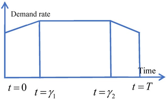Figure 1. Pictorial representation of trapezoidal demand pattern function of the demand rate.

(iii)

The deterioration rate $\theta \left(0<\theta <<1\right)$ is constant.

(iv)

To prevent the decaying rate, deterioration reduction technology is incorporated on the item, and a preservation technology functions $m\left(\xi \right)=\frac{a_1\xi }{1+a_1\xi },a_1>0$ or $m\left(\xi \right)=1-\exp (-a_2\xi ),a_2>0$ is considered Hsu et al. [59], Hasan et al. [60], Masud et al. [61], Dye [42], Yang et al. [62], and Das et al. [56,63]. It should be noted that $m\left(\xi \right)$ is an increasing function with $m^{″}\left(\xi \right)<0$.

(v)

Various costs related to inventory, like purchasing cost, holding cost, ordering cost are known and interval types due to the uncertainty of marketing price.

(vi)

Shortages are allowed and it is completely backlogged.

4. Mathematical Formulation

It is assumed that before the beginning of an inventory cycle, an enterprise makes an order of $(S+R)$ units of a perishable item. After receiving the lot at the beginning (t = 0), $R$ units are utilized to satisfy the backlogged quantities of an earlier cycle and the remaining stock becomes S units. After that, the level of inventory gradually decreases due to the combined effects of deterioration and customers’ requirements. Finally, at the time point, $t=t_1,$ the level of inventory reaches zero. Thereafter, the stock-out situation occurs and at the end of the cycle i.e., at time point $t=T$ along with the maximum shortage $R$ units. Then the entire cycle is repeating itself.

According to the assumptions, the behavior of inventory level at any time $t$ can be presented with the help of the following differential Equations:

$$q^{\prime }(t)=-D(t)-\theta \left\{1-m(\xi )\right\}q(t),0\le t\le t_1$$

(1)

$$q^{\prime }(t)=-D(t),t_1<t\le T$$

(2)

with $q(t_1)=0$.

From the demand function, one can easily obtain the relations ${\gamma }_1=(c-a)/b$, and ${\gamma }_2=T-(c-a)/e_1.$ Depending upon the time $t_1,{\gamma }_1\mathrm{and}{\gamma }_2$, three cases may arise:

Case-I: $0\le t_1\le {\gamma }_1$

Case-II: ${\gamma }_1<t_1\le {\gamma }_2$

Case-III:${\gamma }_2<{\mathrm{t}}_1\le T$

Now, all the cases are discussed in detail.

Case-I: $0\le t_1\le {\gamma }_1$

The level of inventory depletes due to the trapezoidal type of demand and constant decaying rate with preservation technology during the time period $\left[0,t_1\right]$ and it becomes empty at time $t=t_1$ (see Figure 2). Then from Equations (1) and (2), one can write

$$q^{\prime }(t)=-(a+bt)-kq(t),0<t\le t_1$$

(3)

$$q^{\prime }(t)=-\delta (a+bt),t_1<t\le {\gamma }_1$$

(4)

$$q^{\prime }(t)=-\delta c,{\gamma }_1<t\le {\gamma }_2$$

(5)

and

$$q^{\prime }(t)=-\delta \left\{c-e_1(t-{\gamma }_2)\right\},{\gamma }_2<t\le T$$

(6)

with the conditions

$$q(0)=S,q(t_1)=0\mathrm{and}q(T)=-R$$

(7)

where $k=\theta \left\{1-m(\xi )\right\}.$

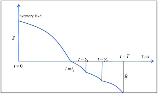
Figure 2. Pictorial representation of inventory situation under Case-I.

The solutions of the differential Equations (3)–(6) with the condition (7) are given by

$$q(t)=-\left(\frac{a+bt}{k}-\frac{b}{k^2}\right)+\left\{\frac{a+b{t}_1}{k}-\frac{b}{k^2}\right\}\exp \left\{k(t_1-t)\right\},0\le t\le t_1$$

(8)

$$q(t)=\delta \left\{a(t_1-t)+\frac{b}{2}(t_1^2-t^2)\right\},t_1<t\le {\gamma }_1$$

(9)

$$q(t)=\delta \left\{c({\gamma }_1-t)+k_1\right\},{\gamma }_1<t\le {\gamma }_2$$

(10)

$$q(t)=\delta \left\{k_2+c{\gamma }_2+\frac{e_1}{2}{\gamma }_2^2-ct+e_1\left(\frac{t^2}{2}-{\gamma }_{2}t\right)\right\},{\gamma }_2<t\le T$$

(11)

where $k=\theta \left\{1-m(\xi )\right\}$

$$k_1=q({\gamma }_1)=a(t_1-{\gamma }_1)+\frac{b}{2}\left(t_1^2-{\gamma }_1^2\right)$$

$$k_2=q({\gamma }_2)=c({\gamma }_1-{\gamma }_2)+k_1$$

$$k_3=c{\gamma }_2+\frac{e_1}{2}{\gamma }_2^2+k_2$$

Again, condition (7) implies

$$S=q(0)=\left(\frac{a+b{t}_1}{k}-\frac{b}{k^2}\right)\exp (k{t}_1)-\left(\frac{a}{k}-\frac{b}{k^2}\right)$$

(12)

As at the time $t=T,q(t)=-R$, so the maximum shortage level R is given by

$$R=\delta \left\{cT-e_1\left(\frac{T^2}{2}-{\gamma }_{2}T\right)-k_2-c{\gamma }_2-\frac{e_1}{2}{\gamma }_2^2\right\}$$

The number of units that deteriorated during the time $[0,t_1]$ is given by

$$\begin{array}{l}{D}^{\prime }=S-{\displaystyle \underset{0}{\overset{t_1}{\int }}D(t)}dt=S-{\displaystyle \underset{0}{\overset{t_1}{\int }}\left(a+bt\right)}dt\\ =S-a{t}_1-\frac{b}{2}{t}_1^2\end{array}$$

(13)

The total salvage value throughout the cycle $T$ is given by $\left[p_L^{\prime },p_U^{\prime }\right]D^{\prime }.$

The bounds of the carrying cost are $C_{hL}{H}_1$ and $C_{hU}{H}_1$, where

$$H_1={\displaystyle \underset{0}{\overset{t_1}{\int }}q(t)}dt=\left(\frac{a+b{t}_1}{k^2}-\frac{b}{k^3}\right)\left\{\exp (k{t}_1)-1\right\}-\frac{a{t}_1}{k}+\frac{b{t}_1}{k^2}+\frac{b{t}_1^2}{2k}$$

Again, the total shortage of units throughout the entire cycle $\left[t_1,T\right]$ are given by

$$\begin{array}{l}SC=-{\displaystyle \underset{t_1}{\overset{T}{\int }}q(t)}dt=-{\displaystyle \underset{t_1}{\overset{{\gamma }_1}{\int }}q(t)}dt-{\displaystyle \underset{{\gamma }_1}{\overset{{\gamma }_2}{\int }}q(t)}dt-{\displaystyle \underset{{\gamma }_2}{\overset{T}{\int }}q(t)}dt\\ =\delta \left\{a{\gamma }_1\left(\frac{{\gamma }_1}{2}-t_1\right)+\frac{b{\gamma }_1}{2}\left(\frac{{\gamma }_1^2}{3}-t_1^2\right)+a\frac{t_1^2}{2}+\frac{b}{3}{t}_1^3\right\}+\delta \left\{c{\gamma }_2\left(\frac{{\gamma }_2}{2}-{\gamma }_1\right)-k_1{\gamma }_2+\frac{c}{2}{\gamma }_1^2+k_1{\gamma }_1\right\}\\ +\delta \left\{\frac{c{T}^2}{2}-e_1{T}^2(\frac{T}{6}-\frac{{\gamma }_2}{2})-k_{3}T-\frac{c}{2}{\gamma }_2^2-e_1\frac{{\gamma }_2^3}{3}+k_3{\gamma }_2\right\}\end{array}$$

The total shortage cost for the entire cycle is $\left[c_{bL},c_{bU}\right]SC.$

Lost sale cost,

$$\begin{array}{l}\left[{\mathrm{LSC}}_L,LS{C}_U\right]=\left[c_{lL},c_{lU}\right](1-\delta )\left[{\displaystyle \underset{t_1}{\overset{{\gamma }_1}{\int }}(a+bt)}dt+{\displaystyle \underset{{\gamma }_1}{\overset{{\gamma }_2}{\int }}c}dt+{\displaystyle \underset{{\gamma }_2}{\overset{T}{\int }}\left\{c-e_1(t-{\gamma }_2)\right\}}dt\right]\\ =\left[c_{lL},c_{lU}\right](1-\delta )\left[a({\gamma }_1-t_1)+\frac{b}{2}\left({\gamma }_1^2-t_1^2\right)+c(T-{\gamma }_1)-\frac{e_1}{2}{(T-{\gamma }_2)}^2\right]\end{array}$$

Thus the bounds of lost sale cost are

$${\mathrm{LSC}}_L=c_{lL}(1-\delta )\left[a({\gamma }_1-t_1)+\frac{b}{2}\left({\gamma }_1^2-t_1^2\right)+c(T-{\gamma }_1)-\frac{e_1}{2}{(T-{\gamma }_2)}^2\right]$$

and

$${\mathrm{LSC}}_U=c_{lU}(1-\delta )\left[a({\gamma }_1-t_1)+\frac{b}{2}\left({\gamma }_1^2-t_1^2\right)+c(T-{\gamma }_1)-\frac{e_1}{2}{(T-{\gamma }_2)}^2\right]$$

Preservation cost $=\zeta T$ per cycle

Ordering cost $=\left[C_{0L},C_{0U}\right]$ per cycle

$$\mathrm{Sales}\mathrm{revenue}(SR)=p{\displaystyle \underset{0}{\overset{t_1}{\int }}D(t)}dt+pR=p{\displaystyle \underset{0}{\overset{t_1}{\int }}\left(a+bt\right)}dt+pR=p\left(a{t}_1+\frac{b{t}_1^2}{2}\right)+pR$$

System Cost:

The total system cost is given by

$$\left[T{C}_L,T{C}_U\right]$$

where $T{C}_L=C_{0L}+C_{pL}(S+R)+C_{hL}{H}_1+c_{bL}SC+{\mathrm{LSC}}_L+\zeta T$, and $T{C}_U=C_{0U}+C_{pU}(S+R)+C_{hU}{H}_1+c_{bU}SC+{\mathrm{LSC}}_U+\zeta T.$

Profit Function:

So, the profit function per unit time $Z$ with respect to two variables $t_1$ and $\xi .$

Hence, the profit per unit time is given by $\left[Z_L\left(t_1,\xi \right),Z_U\left(t_1,\xi \right)\right]$, where $Z_L\left(t_1,\xi \right)=\frac{1}{T}\left[SR+p_L^{\prime }{D}^{\prime }-T{C}_U\right]$ and $Z_U\left(t_1,\xi \right)=\frac{1}{T}\left[SR+p_U^{\prime }{D}^{\prime }-T{C}_L\right]$.

Therefore, the related optimization problem can be written as:

Maximize $\left[Z_L\left(t_1,\xi \right),Z_U\left(t_1,\xi \right)\right]$,

With the conditions $t_1,\xi >0$.

Case-II: ${\gamma }_1<t_1\le {\gamma }_2$

In this case, from the starting point of the cycle, the level of inventory depletes due to the trapezoidal type demand and constant deterioration rate with preservation technology throughout the time period $\left[0,t_1\right]$ and it reaches zero level at the time $t=t_1$ (see Figure 3). Then, from Equations (1) and (2), we have

$$q^{\prime }(t)=-(a+bt)-kq(t),0\le t\le {\gamma }_1$$

(14)

$$q^{\prime }(t)=-c-kq(t),{\gamma }_1<t\le t_1$$

(15)

$$q^{\prime }(t)=-\delta c,t_1<t\le {\gamma }_2$$

(16)

and

$$q^{\prime }(t)=-\delta \left\{c-e_1(t-{\gamma }_2)\right\},{\gamma }_2<t\le T$$

(17)

with

$$q(t)=S\mathrm{at}t=0\mathrm{and}q(t)=0\mathrm{at}$$

(18)

where $k=\theta \left\{1-m(\xi )\right\}.$

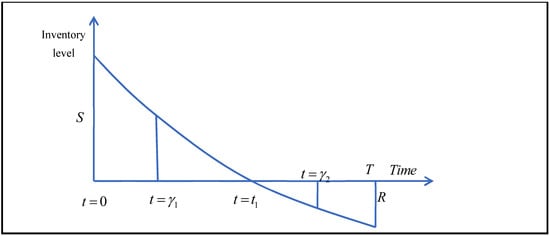
Figure 3. Pictorial representation of inventory situation under Case-II.

The solutions of the differential Equations (14)–(17) with the condition (18) are given by

$$q(t)=-\frac{a}{k}-\frac{bt}{k}+\frac{b}{k^2}+\left\{S+\frac{a}{k}-\frac{b}{k^2}\right\}\exp \left(-kt\right),0<t\le {\gamma }_1$$

(19)

$$q(t)=\frac{c}{k}\left[\exp \left\{k(t_1-t)\right\}-1\right],{\gamma }_1<t\le t_1$$

(20)

$$q(t)=c\delta (t_1-t),t_1<t\le {\gamma }_2$$

(21)

$$q(t)=\delta \left\{-ct+e_1\left(\frac{t^2}{2}-{\gamma }_{2}t\right)+k_3\right\},{\gamma }_2<t\le T$$

(22)

where $k=\theta \left\{1-m(\xi )\right\}$

$$\begin{array}{l}{k}_1=\left[\frac{c}{k}\left[\exp \left\{k(t_1-{\gamma }_1)\right\}-1\right]+\frac{a}{k}+\frac{b{\gamma }_1}{k}-\frac{b}{k^2}\right]\exp (k{\gamma }_1)\\ k_2=q({\gamma }_2)=c(t_1-{\gamma }_2)\\ \mathrm{and}{k}_3=k_2+\left\{c{\gamma }_2+e_1\frac{{\gamma }_2^2}{2})\right\}\end{array}$$

Now, $q(t)=S$ at $t=0$ implies

$$S=q(0)=\frac{b}{k^2}-\frac{a}{k}+k_1$$

(23)

At the time $t=T,\text{\hspace{0.17em}\hspace{0.17em}}q(t)=-R,$ so the highest shortage level R is given by

$$R=\delta \left\{cT-e_1\left(\frac{T^2}{2}-{\gamma }_{2}T\right)-k_3\right\}$$

The total number of units that deteriorate throughout the period $[0,t_1]$ is given by

$$\begin{array}{l}{D}^{\prime }=S-{\displaystyle \underset{0}{\overset{t_1}{\int }}D(t)}dt=S-{\displaystyle \underset{0}{\overset{{\gamma }_1}{\int }}\left(a+bt\right)}dt-{\displaystyle \underset{{\gamma }_1}{\overset{t_1}{\int }}c}dt\\ =S-a{\gamma }_1-\frac{b}{2}{\gamma }_1^2-c(t_1-{\gamma }_1)\end{array}$$

(24)

The total salvage value throughout the cycle time is $\left[{p^{\prime }}_L,{p^{\prime }}_U\right]D^{\prime }.$

The bounds of the carrying cost of the system are $C_{hL}{H}_2$ and $C_{hU}{H}_2$ where

$$\begin{array}{l}{H}_2={\displaystyle \underset{0}{\overset{t_1}{\int }}q(t)}dt={\displaystyle \underset{0}{\overset{{\gamma }_1}{\int }}q(t)}dt+{\displaystyle \underset{{\gamma }_1}{\overset{t_1}{\int }}q(t)}dt\\ =\left[-\frac{a{\gamma }_1}{k}-\frac{b}{2k}{\gamma }_1^2+\frac{b{\gamma }_1}{k^2}+\frac{1}{k}\left(S+\frac{a}{k}-\frac{b}{k^2}\right)\left\{1-\exp (-k{\gamma }_1)\right\}\right]+\frac{c}{k^2}\left[\exp \left\{k(t_1-{\gamma }_1)\right\}-k(t_1-{\gamma }_1)-1\right]\end{array}$$

(25)

The total shortage unit throughout the period $\left[t_1,T\right]$ is given by

$$\begin{array}{l}SC=-{\displaystyle \underset{t_1}{\overset{T}{\int }}q(t)}dt=-{\displaystyle \underset{t_1}{\overset{{\gamma }_2}{\int }}q(t)}dt-{\displaystyle \underset{{\gamma }_2}{\overset{T}{\int }}q(t)}dt\\ =\frac{c\delta }{2}{\left({\gamma }_2-t_1\right)}^2+\delta \left\{\frac{c{T}^2}{2}-e_1\left(\frac{T^3}{6}-\frac{{\gamma }_2{T}^2}{2}\right)-k_{3}T\right\}-\delta \left\{\frac{c{\gamma }_2^2}{2}-e_1\frac{{\gamma }_2^3}{6}-k_3{\gamma }_2\right\}\end{array}$$

(26)

Preservation cost $=\zeta T$ per cycle.

Ordering cost $=\left[C_{0L},C_{0U}\right]$ per cycle.

The total shortage cost for the entire cycle $T$ is $\left[c_{bL},c_{bU}\right]SC.$

Lost sale cost, $\left[{\mathrm{LSC}}_L,{\mathrm{LSC}}_U\right]=\left[c_{lL},c_{lU}\right](1-\delta )\left[{\displaystyle \underset{t_1}{\overset{{\gamma }_2}{\int }}c}dt+{\displaystyle \underset{{\gamma }_2}{\overset{T}{\int }}\left\{c-e_1(t-{\gamma }_2)\right\}}dt\right]$$=\left[c_{lL},c_{lU}\right](1-\delta )\left[c(T-t_1)-\frac{e_1}{2}{(T-{\gamma }_2)}^2\right]$.

Thus, the bounds of lost sale cost are

$$\left[{\mathrm{LSC}}_L,{\mathrm{LSC}}_U\right]=\left[c_{lL}(1-\delta )\left\{c(T-t_1)-\frac{e_1}{2}{(T-{\gamma }_2)}^2\right\},c_{lU}(1-\delta )\left\{c(T-t_1)-\frac{e_1}{2}{(T-{\gamma }_2)}^2\right\}\right]$$

$$\mathrm{Sales}\mathrm{revenue}(SR)=p{\displaystyle \underset{0}{\overset{t_1}{\int }}D(t)}dt+pR=p\left\{{\displaystyle \underset{0}{\overset{{\gamma }_1}{\int }}\left(a+bt\right)}dt+{\displaystyle \underset{{\gamma }_1}{\overset{t_1}{\int }}c}dt\right\}+pR=p\left\{a{\gamma }_1+\frac{b{\gamma }_1^2}{2}+c\left(t_1-{\gamma }_1\right)\right\}+pR$$

System Cost:

The total system cost is given by $\left[T{C}_L,T{C}_U\right]$, where $T{C}_L=C_{0L}+C_{pL}(S+R)+C_{hL}{H}_2+c_{bL}SC+{\mathrm{LSC}}_L+\zeta T$ and $T{C}_U=C_{0U}+C_{pU}(S+R)+C_{hU}{H}_2+c_{bU}SC++{\mathrm{LSC}}_U+\zeta T.$

Profit Function:

So, the profit function $Z$ is a function of two variables $t_1$ and $\xi .$

Hence, the profit function can be written as $\left[Z_L\left(t_1,\xi \right),Z_U\left(t_1,\xi \right)\right]$, where $Z_L\left(t_1,\xi \right)=\frac{1}{T}\left[SR+p_L^{\prime }{D}^{\prime }-T{C}_U\right]$ and $Z_U\left(t_1,\xi \right)=\frac{1}{T}\left[SR+p_U^{\prime }{D}^{\prime }-T{C}_L\right].$

Again, the corresponding optimization problem is given by

Maximize $\left[Z_L\left(t_1,\xi \right),Z_U\left(t_1,\xi \right)\right]$,

Subject to $t_1,\xi >0$.

Case-III: ${\gamma }_2<t_1\le T$

In this case, from the starting of the entire cycle, the inventory level depletes due to the combined effect of constant decaying rate with preservation technology and demand of an item throughout the time period $\left[0,t_1\right]$. Finally, it reaches to empty level at the time $t=t_1$ (see Figure 4). Then from Equations (1) and (2), we have

$$q^{\prime }(t)=-(a+bt)-kq(t),0<t\le {\gamma }_1$$

(27)

$$q^{\prime }(t)=-c-kq(t),{\gamma }_1<t\le {\gamma }_2$$

(28)

$$q^{\prime }(t)=-\left\{c-e_1(t-{\gamma }_2)\right\}-kq(t),{\gamma }_2<t\le t_1$$

(29)

$$\mathrm{and}{q}^{\prime }(t)=-\delta \left\{c-e_1(t-{\gamma }_2)\right\},t_1<t\le T$$

(30)

with

$$q(0)=S,q(t_1)=0\mathrm{and}q(T)=-R.$$

(31)

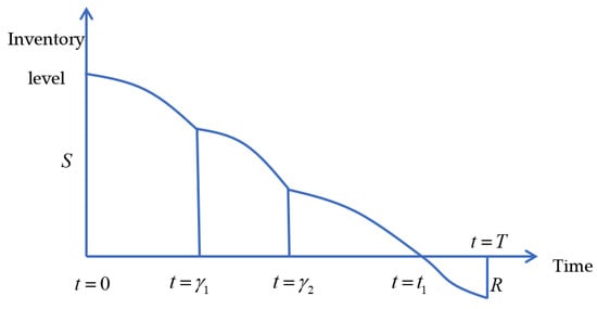
Figure 4. Pictorial representation of inventory situation under Case-III ${\gamma }_2<t_1\le T$.

$q(t)$ is also continuous at $t={\gamma }_1\mathrm{and}{\gamma }_2.$

Solving the differential Equations (27)–(30) with the conditions (31) are given by

$$q(t)=-\frac{a}{k}-\frac{bt}{k}+\frac{b}{k^2}+(S+\frac{a}{k}-\frac{b}{k^2})\exp (-kt),0<t\le {\gamma }_1$$

(32)

$$q(t)=-\frac{c}{k}+k_4\exp \left\{k({\gamma }_2-t)\right\},{\gamma }_1<t\le {\gamma }_2$$

(33)

$$q(t)=-\left[\frac{c}{k}-\frac{e_1(t-{\gamma }_2)}{k}+\frac{e_1}{k^2}\right]+k_1\exp \left\{k(t_1-t)\right\},{\gamma }_2<t\le t_1$$

(34)

$$q(t)=\delta \left\{-ct+e_1\left(\frac{t^2}{2}-{\gamma }_{2}t\right)+k_7-R\right\},t_1<t\le T$$

(35)

where $k=\theta \left\{1-m(\xi )\right\},$

$$k_1=\frac{c}{k}-\frac{e_1(t_1-{\gamma }_2)}{k}+\frac{e_1}{k^2},$$

$$k_2=\frac{c}{k}+\frac{e_1}{k^2},$$

$$k_3=-k_2+k_1\exp \left\{k(t_1-{\gamma }_2)\right\},$$

$$k_4=k_3+\frac{c}{k},$$

$$k_5=-\frac{c}{k}+k_4\exp \left\{k\left({\gamma }_2-{\gamma }_1\right)\right\},$$

$$k_6=\frac{a}{k}+\frac{b{\gamma }_1}{k}-\frac{b}{k^2},$$

$$k_7=cT-e_1\left(\frac{T^2}{2}-{\gamma }_{2}T\right).$$

Now, $q(0)=S$ implies

$$S=\left(k_5+k_6\right)\exp (k{\gamma }_1)-\frac{a}{k}+\frac{b}{k^2}$$

(36)

At the time $t=T,\text{\hspace{0.17em}\hspace{0.17em}}q(t)=-R$, so the highest shortage level R is given by

$$R=\delta \left\{k_7-c{t}_1+e_1\left(\frac{t_1^2}{2}-{\gamma }_2{t}_1\right)\right\}$$

The total number of units deteriorated throughout the time $t=0$ to $t=t_1$ is

$$D^{\prime }=S-{\displaystyle \underset{0}{\overset{t_1}{\int }}D(t)}dt=S-\left[a{\gamma }_1+b\frac{{\gamma }_1^2}{2}+c\left(t_1-{\gamma }_1\right)-\frac{e_1}{2}{\left(t_1-{\gamma }_2\right)}^2\right]$$

(37)

The total salvage value throughout the period is $\left[p_L^{\prime },p_U^{\prime }\right]D^{\prime }.$

The bounds of the carrying cost of the system are $C_{hL}{H}_3$ and $C_{hU}{H}_3$ where

$$\begin{array}{l}{H}_3={\displaystyle \underset{0}{\overset{t_1}{\int }}q(t)}dt={\displaystyle \underset{0}{\overset{{\gamma }_1}{\int }}q(t)}dt+{\displaystyle \underset{{\gamma }_1}{\overset{{\gamma }_2}{\int }}q(t)}dt+{\displaystyle \underset{{\gamma }_2}{\overset{t_1}{\int }}q(t)}dt\\ =\frac{1}{k}\left(S+\frac{a}{k}-\frac{b}{k^2}\right)\left\{1-\exp (-k{\gamma }_1)\right\}-\left(\frac{a{\gamma }_1}{k}+\frac{b{\gamma }_1^2}{2k}-\frac{b{\gamma }_1}{k^2}\right)+\frac{k_4}{k}\left[\exp \left\{k({\gamma }_2-{\gamma }_1)\right\}-1\right]-\frac{c}{k}\left(({\gamma }_2-{\gamma }_1)\right)\\ +\frac{k_1}{k}\left[\exp \left\{k(t_1-{\gamma }_2)\right\}-1\right]-\left[\frac{c}{k}\left(t_1-{\gamma }_2\right)-\frac{e_1}{2k}{\left(t_1-{\gamma }_2\right)}^2+\frac{e_1}{k^2}\left(t_1-{\gamma }_2\right)\right]\end{array}$$

The total shortage of units throughout the period $\left[t_1,T\right]$ is given by

$$SC=-{\displaystyle \underset{t_1}{\overset{T}{\int }}q(t)}dt=\delta \left\{\left(R-k_7\right)(T-t_1)+\frac{1}{2}\left(c-{\gamma }_2\right)\left(T^2-t_1^2\right)-\frac{e_1}{6}\left(T^3-t_1^3\right)\right\}$$

Preservation cost $=\zeta T$ per cycle,

Ordering cost $=\left[C_{0L},C_{0U}\right]$ per cycle,

The total shortage cost for the entire cycle $T$ is $\left[c_{bL},c_{bU}\right]SC.$

The lost sale cost is given by

$$\left[{\mathrm{LSC}}_L,LS{C}_U\right]=\left[c_{lL},c_{lU}\right](1-\delta )\left[{\displaystyle \underset{t_1}{\overset{T}{\int }}\left\{c-e_1(t-{\gamma }_2)\right\}}dt\right]=\left[c_{lL},c_{lU}\right](1-\delta )\left[c(T-t_1)-\frac{e_1}{2}\left\{{(T-{\gamma }_2)}^2-{(t_1-{\gamma }_2)}^2\right\}\right]$$

Thus, the bounds of lost sale cost are

$${\mathrm{LSC}}_L=c_{lL}(1-\delta )\left[c(T-t_1)-\frac{e_1}{2}\left\{{(T-{\gamma }_2)}^2-{(t_1-{\gamma }_2)}^2\right\}\right]$$

and ${\mathrm{LSC}}_U=c_{lU}(1-\delta )\left[c(T-t_1)-\frac{e_1}{2}\left\{{(T-{\gamma }_2)}^2-{(t_1-{\gamma }_2)}^2\right\}\right]$.

Sales revenue (SR) $=p{\displaystyle \underset{0}{\overset{t_1}{\int }}D(t)}dt+pR$$=p\left[a{\gamma }_1+\frac{b{\gamma }_1^2}{2}+c\left(t_1-{\gamma }_1\right)-\frac{e_1}{2}{\left(t_1-{\gamma }_2\right)}^2\right]+pR$

System Cost:

The total system cost is given by $\left[T{C}_L,T{C}_U\right]$, where $T{C}_L=C_{0L}+C_{pL}(S+R)+C_{hL}{H}_3+c_{bL}SC+{\mathrm{LSC}}_L+\zeta T$ and $T{C}_U=C_{0U}+C_{pU}(S+R)+C_{hU}{H}_3+c_{bU}SC+{\mathrm{LSC}}_U+\zeta T.$

Profit Function:

So, the profit function $Z$ is a function concerning two variables $t_1$ and $\xi .$

Hence, the profit per unit time can be written as $\left[Z_L\left(t_1,\xi \right),Z_U\left(t_1,\xi \right)\right]$, where $Z_L\left(t_1,\xi \right)=\frac{1}{T}\left[SR+p_L^{\prime }{D}^{\prime }-T{C}_U\right]$ and $Z_U\left(t_1,\xi \right)=\frac{1}{T}\left[SR+p_U^{\prime }{D}^{\prime }-T{C}_L\right].$

Again, the related optimization problem can be written as

$$\mathrm{Maximize}\left[Z_L\left(t_1,\xi \right),Z_U\left(t_1,\xi \right)\right]$$

(38)

subject to $t_1,{\gamma }_2,\xi >0\mathrm{and}{t}_1>{\gamma }_2.$

5. Numerical Illustration

To validate and also to illustrate the proposed models, three numerical examples are considered and solved. The best-found solutions for the feasible cases of each example are shown in Tables 2–10. To solve each optimization problem of the hypothetical inventory model, different variants of QPSO, viz. GQPSO, AQPSO, and WQPSO techniques are used and these algorithms are coded in C language. The corresponding computational works are performed on a laptop with the configuration Intel core i-3 with 2.40 GHz 7th generation processor in the Linux operating system. Every algorithm is run 50 times independently to solve each example. It is also to be mentioned that the obtained results are called best-found solutions which are either optimal or nearer to the optimal solution. The corresponding results of these computations are shown in Tables 2–4 for Example 1, Tables 5–7 for Example 2, and Tables 8–10 for Example 3.

Example 1.

The values of different parameters of the proposed models are as follows:

$C_{pL}=\$12$/unit,$C_{pU}=\$14$/unit,$p=\$32$/unit,$a=15$,$b=2.8$,$c=70$,$C_{0L}=\$95$/order,$C_{0U}=\$105/\mathrm{order}$,$e_1=15$,$C_{hL}=\$0.9$/unit,$C_{hU}=\$1.1$/unit,$\theta =0.1$,$a_2=0.1$,$c_{bL}=\$1.5$/unit/unit time,$c_{bU}=\$2.5$/unit/unit time,$p_L^{\prime }=\$7.5$/unit,$p_U^{\prime }=\$9.5$,$c_{lL}=\$0.7$,$c_{lU}=\$0.9$,$\delta =0.2$and$T=24$weeks.

For the above hypothetical data, Case-I is feasible whereas the rest two cases are infeasible. It indicates that the other constraints are not satisfied with this particular example. The best-found, worst found solutions and statistical results are shown in Table 2, Table 3 and Table 4.

Table 2. Best found results for Case-I of Example 1.

Types of QPSO	${\mathit{Z}}_{\mathit{L}}$ (in $)	${\mathit{Z}}_{\mathit{U}}$ (in $)	${\mathit{Z}}_{\mathit{C}}$ (in $)	${\mathit{Z}}_{\mathit{r}}$	${\mathit{t}}_1$ (Weeks)	${\mathit{\gamma }}_1$ (Weeks)	${\mathit{\gamma }}_2$ (Weeks)	$\mathit{\xi }$	$\mathit{S}$	$\mathit{R}$	Computational Time (s)
GQPSO	145.4559	289.9762	217.7161	72.26013	17.6825	19.6429	20.3333	35.5954	724.7227	67.2026	0.0308
AQPSO	145.456	289.9762	217.7161	72.26011	17.6825	19.6429	20.3333	35.5954	724.7224	67.2027	0.0221
WQPSO	145.456	289.9762	217.7161	72.2601	17.6825	19.6429	20.3333	35.5954	724.7223	67.2027	0.0542

Table 3. Worst found results for Case-I of Example 1.

Types of QPSO	${\mathit{Z}}_{\mathit{L}}$ (in $)	${\mathit{Z}}_{\mathit{U}}$ (in $)	${\mathit{Z}}_{\mathit{C}}$ (in $)	${\mathit{Z}}_{\mathit{r}}$	${\mathit{t}}_1$ (Weeks)	${\mathit{\gamma }}_1$ (Weeks)	${\mathit{\gamma }}_2$ (Weeks)	$\mathit{\xi }$	$\mathit{S}$	$\mathit{R}$	Computational Time (s)
GQPSO	145.456	289.9762	217.7161	72.26011	17.6825	19.6429	20.3333	35.5954	724.7227	67.2027	0.037
AQPSO	145.456	289.9762	217.7161	72.26012	17.6825	19.6429	20.3333	35.5954	724.7225	67.2027	0.0287
WQPSO	145.456	289.9762	217.7161	72.2601	17.6825	19.6429	20.3333	35.5954	724.7224	67.2027	0.0656

Table 4. Statistical Analysis for various types of QPSO for Case-I of Example 1.

Types of QPSO	$\mathbf{Best}\mathbf{Found}{\mathit{Z}}_{\mathit{C}}$ (in $)	$\mathbf{Worst}\mathbf{Found}{\mathit{Z}}_{\mathit{C}}$ (in $)	$\mathbf{Mean}\mathbf{of}{\mathit{Z}}_{\mathit{C}}$ (in $)	Standard Deviation
GQPSO	217.7161	217.7161	217.7161	0
AQPSO	217.7161	217.7161	217.7161	0
WQPSO	217.7161	217.7161	217.7161	0

Example 2.

The values of different parameters are given as follows:

$C_{pL}=\$12$/unit,$C_{pU}=\$14$/unit,$p=\$32$/unit,$a=15$,$b=10$,$c=65$,$C_{0L}=\$95$/order,$C_{0U}=\$105/\mathrm{order}$,$e_1=15$,$C_{hL}=\$0.9$/unit,$C_{hU}=\$1.1$/unit,$\theta =0.1$,$a_2=0.1$,$c_{bL}=\$1.5$/unit/unit time,$c_{bU}=\$2.5$/unit/unit time,$p_L^{\prime }=\$7.5$/unit,$p_U^{\prime }=\$9.5$,$c_{lL}=\$0.7$,$c_{lU}=\$0.9$,$\delta =0.2$and$T=24$weeks.

For the above hypothetical data, Case-II is feasible whereas the rest two cases are infeasible. It indicates that the other constraints are not satisfied with this particular example. The best-found, worst found solutions and statistical results are shown in Table 5, Table 6 and Table 7.

Table 5. Best found solutions for Case-II of Example 2.

Types of QPSO	${\mathit{Z}}_{\mathit{L}}$ (in $)	${\mathit{Z}}_{\mathit{U}}$ (in $)	${\mathit{Z}}_{\mathit{C}}$ (in $)	${\mathit{Z}}_{\mathit{r}}$	${\mathit{\gamma }}_1$ (Weeks)	${\mathit{t}}_1$ (Weeks)	${\mathit{\gamma }}_2$ (Weeks)	$\mathit{\xi }$	$\mathit{S}$	$\mathit{R}$	Computational Time (s)
GQPSO	271.0675	463.4415	367.2545	96.18704	5.0000	17.7892	20.6667	38.1136	1053.8824	64.0743	0.0087
AQPSO	271.0675	463.4415	367.2545	96.18699	5.0000	17.7891	20.6667	38.1136	1053.8817	64.0744	0.0054
WQPSO	271.0675	463.4415	367.2545	96.18699	5.0000	17.7891	20.6667	38.1136	1053.8818	64.0744	0.0123

Table 6. Worst found results for Case-II of Example 2.

Types of QPSO	${\mathit{Z}}_{\mathit{L}}$ (in $)	${\mathit{Z}}_{\mathit{U}}$ (in $)	${\mathit{Z}}_{\mathit{C}}$ (in $)	${\mathit{Z}}_{\mathit{r}}$	${\mathit{\gamma }}_1$ (Weeks)	${\mathit{t}}_1$ (Weeks)	${\mathit{\gamma }}_2$ (Weeks)	$\mathit{\xi }$	$\mathit{S}$	$\mathit{R}$	Computational Time (s)
GQPSO	271.0675	463.4415	367.2545	96.18699	5.0000	17.7891	20.6667	38.1136	1053.8817	64.0744	0.0098
AQPSO	271.0675	463.4415	367.2545	96.187	5.0000	17.7892	20.6667	38.1136	1053.8818	64.0744	0.0062
WQPSO	271.0675	463.4415	367.2545	96.18699	5.0000	17.7891	20.6667	38.1136	1053.8818	64.0744	0.0163

Table 7. Statistical analysis for different types of QPSO for Case-II of Example 2.

Types of QPSO	$\mathbf{Best}\mathbf{Found}{\mathit{Z}}_{\mathit{C}}$ (in $)	$\mathbf{Worst}\mathbf{Found}{\mathit{Z}}_{\mathit{C}}$ (in $)	$\mathbf{Mean}\mathbf{of}{\mathit{Z}}_{\mathit{C}}$ (in $)	Standard Deviation
GQPSO	367.2545	367.2545	367.2545	0
AQPSO	367.2545	367.2545	367.2545	0
WQPSO	367.2545	367.2545	367.2545	0

Example 3.

The input values of different system parameters are given as follows:

$C_{pL}=\$12$/unit,$C_{pU}=\$14$/unit,$p=\$32$/unit,$a=15$,$b=40$,$c=85$,$C_{0L}=\$95$/order,$C_{0U}=\$105/\mathrm{order}$,$e_1=3.5$,$C_{hL}=\$0.9$/unit,$C_{hU}=\$1.1$/unit,$\theta =0.1$,$a_2=0.1$,$c_{bL}=\$1.5$/unit/unit time,$c_{bU}=\$2.5$/unit/unit time,${p^{\prime }}_L=\$7.5$/unit,${p^{\prime }}_U=\$9.5$,$c_{lL}=\$0.7$,$c_{lU}=\$0.9$,$\delta =0.2$and$T=24$weeks.

For the above hypothetical data, Case-III is feasible whereas the rest two cases are infeasible. It indicates that the other constraints are not satisfied with this particular example. The best-found, worst found and statistical results are shown in Table 8, Table 9 and Table 10.

Table 8. Best found results for Case-III of Example 3.

Types of QPSO	${\mathit{Z}}_{\mathit{L}}$ (in $)	${\mathit{Z}}_{\mathit{U}}$ (in $)	${\mathit{Z}}_{\mathit{C}}$ (in $)	${\mathit{Z}}_{\mathit{r}}$	${\mathit{\gamma }}_1$ (Weeks)	${\mathit{\gamma }}_2$ (Weeks)	${\mathit{t}}_1$ (Weeks)	$\mathit{\xi }$	$\mathit{S}$	$\mathit{R}$	Computational Time (s)
GQPSO	345.2759	438.5276	391.9018	46.62583	1.7500	4.0000	6.5651	10.3321	703.4356	158.6968	0.0103
AQPSO	345.2928	438.5107	391.9017	46.60898	1.7500	4.0000	6.5637	9.8094	703.2428	158.7168	0.0054
WQPSO	345.2759	438.5276	391.9018	46.62583	1.7500	4.0000	6.5651	24.0148	703.4356	158.6968	0.0139

Table 9. Worst found results for Case- III of Example 3.

Types of QPSO	${\mathit{Z}}_{\mathit{L}}$ (in $)	${\mathit{Z}}_{\mathit{U}}$ (in $)	${\mathit{Z}}_{\mathit{C}}$ (in $)	${\mathit{Z}}_{\mathit{r}}$	${\mathit{\gamma }}_1$ (Weeks)	${\mathit{\gamma }}_2$ (Weeks)	${\mathit{t}}_1$ (Weeks)	$\mathit{\xi }$	$\mathit{S}$	$\mathit{R}$	Computational Time (s)
GQPSO	345.2759	438.5276	391.9018	46.62583	1.7500	4.0000	6.5651	14.5762	703.4356	158.6968	0.0124
AQPSO	338.219	443.7263	390.9726	52.75365	1.7500	4.0000	7.0334	15.4843	772.9438	151.6534	0.0054
WQPSO	345.2759	438.5276	391.9018	46.62583	1.7500	4.0000	6.5651	13.0511	703.4356	158.6968	0.019

Table 10. Statistical Analysis for different variants of QPSO for Case-III of Example 3.

Types of QPSO	$\mathbf{Best}\mathbf{Found}{\mathit{Z}}_{\mathit{C}}$ (in $)	$\mathbf{Worst}\mathbf{Found}{\mathit{Z}}_{\mathit{C}}$ (in $)	$\mathbf{Mean}\mathbf{of}{\mathit{Z}}_{\mathit{C}}$ (in $)	Standard Deviation
GQPSO	391.9018	391.9018	391.9018	0
AQPSO	391.9017	390.9726	391.714238	0.270107162
WQPSO	391.9018	391.9018	391.9018	0

6. Discussions

• Table 2 and Table 3, represent that the average profit/mid-value of the profit ($Z_C$) obtained by using GQPSO, AQPSO and WQPSO techniques be the same up to certain decimal places. Also, it should be noted that the AQPSO technique takes less computational time to find the best-found solution.
• It is clear from Table 5 and Table 6 that the average profit ($Z_C$) obtained by using GQPSO, AQPSO and WQPSO techniques be the same up to certain decimal places. It is observed that the AQPSO technique takes less time to find the best-found solution. To solve this particular problem AQPSO is taking the least time. It does not give any guarantee that AQPSO always takes less time, it may vary from problem to problem.
• From Table 9 and Table 10, it is also remarked that the average profit obtained by using GQPSO and WQPSO techniques be the same up to certain decimal places although it is different when applying the AQPSO technique. In this case, the AQPSO technique takes less time to find the best-found solution. From Table 4 and Table 7, it is remarked that the statistical results assured that the GQPSO, AQPSO, and WQPSO algorithms equally perform and they are equally efficient to find the best-found solutions for Examples 1 and 2. From Table 10, it is also remarked that the statistical results assured that the GQPSO and WQPSO algorithms equally perform and they are equally efficient to find the best-found solutions for Examples 3.
• From Table 2, Table 5and Table 8, it is remarked that the best-found value of average profit ($Z_C$) of Examples 1, 2, and 3 lie in between the bounds of the best found (optimal) value of interval-valued average profit of Examples 1, 2, and 3. So, the study of the best found (optimal) policy in an interval environment is well validated.

7. Sensitivity Analysis

For Example 2, sensitivity analyses are performed to observe the effect of different parameters on the center of the average profit ($Z_C$), initial inventory level ($S$), maximum shortage level ($R$), stock-in period $(t_1)$, and preservation technology cost $(\xi )$. This experiment is performed by the GQPSO technique and it is obtained by changing each bound of a parameter by −20% to +20% keeping the values of the rest parameters as their original input values. For each problem, the best-found results are taken from 50 independent runs. The detailed analyses are depicted in Figure 5, Figure 6, Figure 7, Figure 8, Figure 9 and Figure 10.

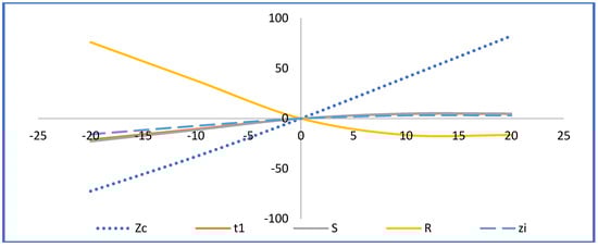
Figure 5. Impact of post optimality analysis of ‘$p$’ on $Z_C$, $t_1$,$S$, $R$, and $\xi$.

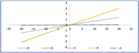
Figure 6. Impact of post optimality analysis of ‘$a$’ on $Z_C$, $t_1$, $S$, $R$, and $\xi$.

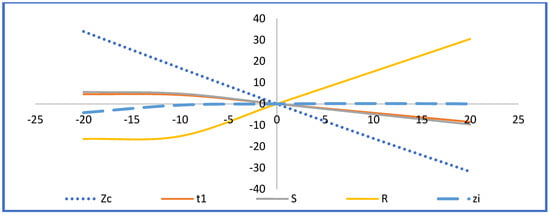
Figure 7. Impact of post optimality analysis of ‘$\left[C_{pL},C_{pU}\right]$’ on $Z_C$, $t_1$, $S$, $R$, and $\xi$.

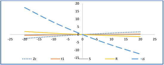
Figure 8. Impact of post optimality analysis of ‘$a_2$’ on $Z_C$, $t_1$, $S$, $R$, and $\xi$.

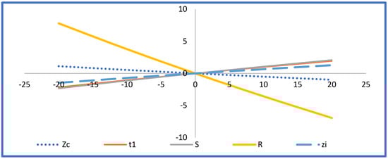
Figure 9. Impact of post optimality analysis of ‘$\left[c_{bL},c_{bU}\right]$’ on $Z_C$,$t_1$, $S$, $R$, and $\xi$.

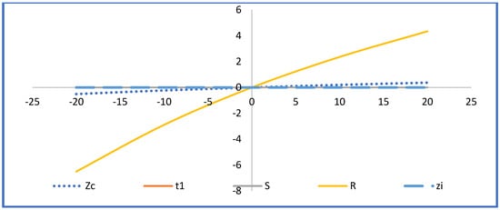
Figure 10. Impact of post optimality analysis of ‘$e_1$’ on $Z_C$, $t_1$, $S$, $R$, and $\xi$.

From the Figure 5, Figure 6, Figure 7, Figure 8, Figure 9 and Figure 10, following implications can be observed.

(i)

The center of average profit ($Z_C$) is highly sensitive w. r. to the selling price ($p$) and interval-valued purchase cost ($\left[C_{pL},C_{pU}\right]$).Again, $Z_C$ is less sensitive w. r. to interval-valued shortage cost ($\left[c_{bL},c_{bU}\right]$), demand parameter, $\left(a\right)$ and preservation parameter ($a_2$) whereas it is insensitive w. r. to demand parameter $\left(e_1\right)$. Further, $\left[C_{pL},C_{pU}\right]$ and $\left[c_{bL},c_{bU}\right]$ both have a reverse effect on the average profit.

(ii)

Stock-in period $(t_1)$ is less sensitive w. r. to the selling price ($p$), purchase cost $\left(\left[C_{pL},C_{pU}\right]\right)$, shortage cost ($\left[c_{bL},c_{bU}\right]$), demand parameter ($a_2$) and demand parameter ($e_1$). Again, T is insensitive with respect to preservation parameter ($a_2$). Further, the parameters ‘$a$’, ‘$\left[C_{pL},C_{pU}\right]$’, ‘$\left[c_{bL},c_{bU}\right]$’, ‘$e_1$’ all have inverse effect on the business period ’$t_1$’.

(iii)

Initial inventory level ($S$) is less sensitive w. r. to purchase cost $\left[C_{pL},C_{pU}\right]$ and with respect to selling price $\left(p\right)$, demand parameter $\left(a\right)$ and $\left(\left[c_{bL},c_{bU}\right]\right)$. Again, it is insensitive with respect to preservation parameter $a_2$ and $e_1$. Further, it is observed that for the positive changes of the parameters ‘$a$’, ‘$\left[c_{bL},c_{bU}\right]$’, ‘$e_1$’, the initial inventory level $\left(S\right)$ changes inversely.

(iv)

The highest shortages level ($R$) is highly sensitive w. r. to selling price $\left(p\right)$ and demand parameter purchase cost $\left(\left[C_{pL},C_{pU}\right]\right)$ but $\left(p\right)$ has the reverse effect on ‘$R$’. Further, it is less impact w.r.to demand parameter $\left(a\right)$, preservation parameter ($a_2$), $\left[c_{bL},c_{bU}\right]$ and demand parameter ($e_1$). Further, it is noted that $\left(p\right)$$\left[c_{bL},c_{bU}\right]$ and have a reverse effect on ‘$R$’.

(v)

Preservation cost ($\xi$) is equally sensitive w. r. to preservation parameter ($a_2$) and it is less sensitive w. r. to the selling price $\left(p\right)$ and w. r. to $\left[c_{bL},c_{bU}\right]$. Again, it is insensitive w. r. to parameters $a$, $\left[C_{pL},C_{pU}\right]$ and $e_1.$

8. Managerial Implications

From the earlier observations, the following managerial insights may be suggested:

• The selling price of the item ($p$) and interval-valued purchasing cost ($\left[C_{pL},C_{pU}\right]$) have a significant impact on the retailer’s profit per unit time. So, the decision-maker should think about the selling price of the item to increase the customers’ demand as well as the smooth running of their business.
• To reduce the natural effect of the deterioration of products in the stock-in situation, preservation technology should be used to increase the average profit of the system.
• The proposed model is more appropriate for seasonal products e.g., fruits, vegetables, seasonal fishes, etc. At the beginning of the season, the demand for such type of the product increases then after a certain period it becomes stable. Finally, the demand for the product declined up to a certain level throughout the business period. So, the business period may be fixed. Keeping in mind this type of behavior of the demand of the sessional product, decision-maker should make the proper business plan to increase their profit.

9. Conclusions

In this study, an inventory model is developed for deteriorating items considering trapezoidal type demand and preservation technology to reduce the deterioration. Shortages are partially backlogged and inventory costs parameters are as interval-valued. Then the corresponding profit maximization problem is developed. Three different variants of QPSO techniques GQPSO, AQPSO, and WQPSO are used to solve this profit maximization problem. Finally, sensitivity analyses are studied graphically for Example 2 to study the impact of different parameters on the best-found policy. Also, from the statistical analysis, it is observed that both the techniques GQPSO and WQPSO are equally efficient to solve the optimization problems with interval-valued objectives.

The proposed trapezoidal type of demand is observed in the case of seasonal products. To reduce the natural phenomenon of deterioration, consideration of preservation technology makes more realistic in the modeling of inventory problems.

This work can be extended in various ways. One may consider the advertisement numbers/ cost, time, selling price as well as displayed stock level dependent demand, nonlinear holding cost, inflation, etc. Furthermore, this work can be extended by considering trade credit policy, discount facility, advance payment policy.

References

- Cheng, M.; Wang, G. A note on the inventory model for deteriorating items with trapezoidal type demand rate. Comput. Ind. Eng. 2009, 56, 1296–1300. [Google Scholar] [CrossRef]
- Cheng, M.; Zhang, B.; Wang, G. Optimal policy for deteriorating items with trapezoidal type demand and partial backlogging. Appl. Math. Model. 2011, 35, 3552–3560. [Google Scholar] [CrossRef]
- Lin, K.-P. An extended inventory models with trapezoidal type demands. Appl. Math. Comput. 2013, 219, 11414–11419. [Google Scholar] [CrossRef]
- Chuang, K.-W.; Lin, C.-N.; Lan, C.-H. Order Policy Analysis for Deteriorating Inventory Model with Trapezoidal Type Demand Rate. J. Netw. 2013, 8, 1838–1844. [Google Scholar] [CrossRef] [Green Version]
- Singh, T.; Pattnayak, H. An EOQ inventory model for deteriorating items with varying trapezoidal type demand rate and Weibull distribution deterioration. J. Inf. Optim. Sci. 2013, 34, 341–360. [Google Scholar] [CrossRef]
- Lin, J.; Hung, K.-C.; Julian, P. Technical note on inventory model with trapezoidal type demand. Appl. Math. Model. 2014, 38, 4941–4948. [Google Scholar] [CrossRef]
- Mishra, U. An inventory model for deteriorating items under trapezoidal type demand and controllable deterioration rate. Prod. Eng. 2015, 9, 351–365. [Google Scholar] [CrossRef]
- Wu, J.; Skouri, K.; Teng, J.-T.; Hu, Y. Two inventory systems with trapezoidal-type demand rate and time-dependent deterioration and backlogging. Expert Syst. Appl. 2016, 46, 367–379. [Google Scholar] [CrossRef]
- Vandana; Srivastava, H.M. An inventory model for ameliorating/deteriorating items with trapezoidal demand and complete backlogging under inflation and time discounting. Math. Methods Appl. Sci. 2016, 40, 2980–2993. [Google Scholar] [CrossRef]
- Wu, J.; Teng, J.-T.; Skouri, K. Optimal inventory policies for deteriorating items with trapezoidal-type demand patterns and maximum lifetimes under upstream and downstream trade credits. Ann. Oper. Res. 2017, 264, 459–476. [Google Scholar] [CrossRef]
- Garai, T.; Chakraborty, D.; Roy, T.K. Fully fuzzy inventory model with price-dependent demand and time varying holding cost under fuzzy decision variables. J. Intell. Fuzzy Syst. 2019, 36, 3725–3738. [Google Scholar] [CrossRef]
- Xu, C.; Zhao, D.; Min, J.; Hao, J. An inventory model for nonperishable items with warehouse mode selection and partial backlogging under trapezoidal-type demand. J. Oper. Res. Soc. 2020, 72, 744–763. [Google Scholar] [CrossRef]
- Kumar, P. Optimal policies for inventory model with shortages, time-varying holding and ordering costs in trapezoidal fuzzy environment. Indep. J. Manag. Prod. 2021, 12, 557–574. [Google Scholar] [CrossRef]
- Kazemi, N.; Ehsani, E.; Jaber, M. An inventory model with backorders with fuzzy parameters and decision variables. Int. J. Approx. Reason. 2010, 51, 964–972. [Google Scholar] [CrossRef] [Green Version]
- De, S.K.; Sana, S.S. Fuzzy order quantity inventory model with fuzzy shortage quantity and fuzzy promotional index. Econ. Model. 2013, 31, 351–358. [Google Scholar] [CrossRef]
- Mondal, M.; Maity, A.K.; Maiti, M.K.; Maiti, M. A production-repairing inventory model with fuzzy rough coefficients under inflation and time value of money. Appl. Math. Model. 2013, 37, 3200–3215. [Google Scholar] [CrossRef]
- Manna, A.K.; Dey, J.K.; Mondal, S.K. Controlling GHG emission from industrial waste perusal of production inventory model with fuzzy pollution parameters. Int. J. Syst. Sci. Oper. Logist. 2017, 6, 368–393. [Google Scholar] [CrossRef]
- De, A.; Khatua, D.; Kar, S. Control the preservation cost of a fuzzy production inventory model of assortment items by using the granular differentiability approach. Comput. Appl. Math. 2020, 39, 1–22. [Google Scholar] [CrossRef]
- Pulido-Rojano, A.; Andrea, A.; Padilla-Polanco, M.; Sánchez-Jiménez, M.; De la-Rosa, L. An optimization approach for inventory costs in probabilistic inventory models: A case study. Ingeniare 2020, 28, 383–395. [Google Scholar] [CrossRef]
- Adak, S.; Mahapatra, G.S. Effect of reliability on varying demand and holding cost on inventory system incorporating probabilistic deterioration. J. Ind. Manag. Optim. 2020, 18, 173–193. [Google Scholar] [CrossRef]
- Dutta, D.; Kumar, P. A partial backlogging inventory model for deteriorating items with time-varying demand and holding cost: An interval number approach. Croat. Oper. Res. Rev. 2015, 6, 321–334. [Google Scholar] [CrossRef]
- Bhunia, A.K.; Shaikh, A.A. Investigation of two-warehouse inventory problems in interval environment under inflation via particle swarm optimization. Math. Comput. Model. Dyn. Syst. 2016, 22, 160–179. [Google Scholar] [CrossRef]
- Bhunia, A.K.; Shaikh, A.A.; Cárdenas-Barrón, L.E. A partially integrated production-inventory model with interval valued inventory costs, variable demand and flexible reliability. Appl. Soft Comput. 2017, 55, 491–502. [Google Scholar] [CrossRef]
- Gupta, R.K.; Bhunia, A.K.; Goyal, S.K. An application of genetic algorithm in a marketing oriented inventory model with interval-valued inventory costs and three-component demand rate dependent on displayed stock level. Appl. Math. Comput. 2007, 192, 466–478. [Google Scholar] [CrossRef]
- Gupta, R.K.; Bhunia, A.; Goyal, S. An application of Genetic Algorithm in solving an inventory model with advance payment and interval valued inventory costs. Math. Comput. Model. 2009, 49, 893–905. [Google Scholar] [CrossRef]
- Chakrabortty, S.; Madhumangal, P.A.L.; Nayak, P.K. An algorithm for solution of an interval-valued EOQ model. Int. J. Optim. Control. Theor. Appl. 2013, 3, 55–64. [Google Scholar] [CrossRef] [Green Version]
- Mondal, R.; Shaikh, A.A.; Bhunia, A.K. Crisp and interval inventory models for ameliorating item with Weibull distributed amelioration and deterioration via different variants of quantum behaved particle swarm optimization-based techniques. Math. Comput. Model. Dyn. Syst. 2019, 25, 602–626. [Google Scholar] [CrossRef]
- Shaikh, A.A.; Cárdenas-Barrón, L.E.; Tiwari, S. A two-warehouse inventory model for non-instantaneous deteriorating items with interval-valued inventory costs and stock-dependent demand under inflationary conditions. Neural Comput. Appl. 2019, 31, 1931–1948. [Google Scholar] [CrossRef]
- Rahman, S.; Manna, A.K.; Shaikh, A.A.; Bhunia, A.K. An application of interval differential equation on a production inventory model with interval-valued demand via center-radius optimization technique and particle swarm optimization. Int. J. Intell. Syst. 2020, 35. [Google Scholar] [CrossRef]
- Ruidas, S.; Seikh, M.R.; Nayak, P.K. A production inventory model with interval-valued carbon emission parameters under price-sensitive demand. Comput. Ind. Eng. 2021, 154, 107154. [Google Scholar] [CrossRef]
- Ghare, P.M.; Schrader, G.F. An inventory model for exponentially deteriorating items. J. Ind. Eng. 1963, 14, 238–243. [Google Scholar]
- Covert, R.P.; Philip, G.C. An EOQ Model for Items with Weibull Distribution Deterioration. AIIE Trans. 1973, 5, 323–326. [Google Scholar] [CrossRef]
- Mahapatra, G.S.; Adak, S.; Mandal, T.K.; Pal, S. Inventory model for deteriorating items with time and reliability dependent demand and partial backorder. Int. J. Oper. Res. 2017, 29, 344–359. [Google Scholar] [CrossRef]
- Shaikh, A.A.; Mashud, A.H.M.; Uddin, M.S.; Khan, M.A.A. Non-instantaneous deterioration inventory model with price and stock dependent demand for fully backlogged shortages under inflation. Int. J. Bus. Forecast. Mark. Intell. 2017, 3, 152–164. [Google Scholar] [CrossRef]
- Shah, N.H.; Naik, M.K. Inventory model for non-instantaneous deterioration and price-sensitive trended demand with learning effects. Int. J. Inventory Res. 2018, 5, 60–77. [Google Scholar] [CrossRef]
- Chen, L.; Chen, X.; Keblis, M.F.; Li, G. Optimal pricing and replenishment policy for deteriorating inventory under stock-level-dependent, time-varying and price-dependent demand. Comput. Ind. Eng. 2019, 135, 1294–1299. [Google Scholar] [CrossRef]
- Mahmoodi, A. Joint pricing and inventory control of duopoly retailers with deteriorating items and linear demand. Comput. Ind. Eng. 2019, 132, 36–46. [Google Scholar] [CrossRef]
- Saha, S.; Sen, N. An inventory model for deteriorating items with time and price dependent demand and shortages under the effect of inflation. Int. J. Math. Oper. Res. 2019, 14, 377–388. [Google Scholar] [CrossRef]
- Khakzad, A.; Gholamian, M.R. The effect of inspection on deterioration rate: An inventory model for deteriorating items with advanced payment. J. Clean. Prod. 2020, 254, 120117. [Google Scholar] [CrossRef]
- Khan, A.-A.; Shaikh, A.A.; Panda, G.C.; Bhunia, A.K.; Konstantaras, I. Non-instantaneous deterioration effect in ordering decisions for a two-warehouse inventory system under advance payment and backlogging. Ann. Oper. Res. 2020, 289, 243–275. [Google Scholar] [CrossRef]
- Xu, C.; Liu, X.; Wu, C.; Yuan, B. Optimal Inventory Control Strategies for Deteriorating Items with a General Time-Varying Demand under Carbon Emission Regulations. Energies 2020, 13, 999. [Google Scholar] [CrossRef] [Green Version]
- Dye, C.-Y. The effect of preservation technology investment on a non-instantaneous deteriorating inventory model. Omega 2012, 41, 872–880. [Google Scholar] [CrossRef]
- Wahab, M.; Mamun, S.; Ongkunaruk, P. EOQ models for a coordinated two-level international supply chain considering imperfect items and environmental impact. Int. J. Prod. Econ. 2011, 134, 151–158. [Google Scholar] [CrossRef]
- Zhao, L. An Inventory Model under Trapezoidal Type Demand, Weibull-Distributed Deterioration, and Partial Backlogging. J. Appl. Math. 2014, 2014, 1–10. [Google Scholar] [CrossRef] [Green Version]
- Taleizadeh, A.A.; Moshtagh, M.S.; Moon, I. Optimal decisions of price, quality, effort level and return policy in a three-level closed-loop supply chain based on different game theory approaches. Eur. J. Ind. Eng. 2017, 11, 486. [Google Scholar] [CrossRef] [Green Version]
- Rahman, M.S.; Duary, A.; Shaikh, A.A.; Bhunia, A.K. An application of parametric approach for interval differential equation in inventory model for deteriorating items with selling-price-dependent demand. Neural Comput. Appl. 2020, 32, 14069–14085. [Google Scholar] [CrossRef]
- Dey, B.K.; Bhuniya, S.; Sarkar, B. Involvement of controllable lead time and variable demand for a smart manufacturing system under a supply chain management. Expert Syst. Appl. 2021, 184, 115464. [Google Scholar] [CrossRef]
- Shaikh, A.A.; Das, S.C.; Bhunia, A.K.; Sarkar, B. Decision support system for customers during availability of trade credit financing with different pricing situations. RAIRO Rech. Opérationnelle 2021, 55, 1043–1061. [Google Scholar] [CrossRef]
- Jabbarzadeh, A.; Aliabadi, L.; Yazdanparast, R. Optimal payment time and replenishment decisions for retailer’s inventory system under trade credit and carbon emission constraints. Oper. Res. 2019, 21, 589–620. [Google Scholar] [CrossRef]
- Singh, S.R.; Rathore, H. Optimal Payment Policy with Preservation Technology Investment and Shortages Under Trade Credit. Indian J. Sci. Technol. 2015, 8, 203. [Google Scholar] [CrossRef]
- Tayal, S.; Singh, S.R.; Sharma, R. An integrated production inventory model for perishable products with trade credit period and investment in preservation technology. Int. J. Math. Oper. Res. 2016, 8, 137. [Google Scholar] [CrossRef]
- Mishra, U.; Tijerina-Aguilera, J.; Tiwari, S.; Cárdenas-Barrón, L.E. Retailer’s Joint Ordering, Pricing, and Preservation Technology Investment Policies for a Deteriorating Item under Permissible Delay in Payments. Math. Probl. Eng. 2018, 2018, 1–14. [Google Scholar] [CrossRef]
- Mishra, U.; Cárdenas-Barrón, L.E.; Tiwari, S.; Shaikh, A.A.; Treviño-Garza, G. An inventory model under price and stock-dependent demand for controllable deterioration rate with shortages and preservation technology investment. Ann. Oper. Res. 2017, 254, 165–190. [Google Scholar] [CrossRef]
- Bardhan, S.; Pal, H.; Giri, B.C. Optimal replenishment policy and preservation technology investment for a non-instantaneous deteriorating item with stock-dependent demand. Oper. Res. 2017, 19, 347–368. [Google Scholar] [CrossRef]
- Shah, N.H.; Chaudhari, U.; Jani, M.Y. Optimal control analysis for service, inventory and preservation technology investment. Int. J. Syst. Sci. Oper. Logist. 2019, 6, 130–142. [Google Scholar] [CrossRef]
- Das, S.C.; Zidan, A.; Manna, A.K.; Shaikh, A.A.; Bhunia, A.K. An application of preservation technology in inventory control system with price dependent demand and partial backlogging. Alex. Eng. J. 2020, 59, 1359–1369. [Google Scholar] [CrossRef]
- Khanna, A.; Jaggi, C.K. An inventory model under price and stock-dependent demand for controllable deterioration rate with shortages and preservation technology investment: Revisited. OPSEARCH 2021, 58, 181–202. [Google Scholar]
- Rahman, S.; Duary, A.; Khan, A.-A.; Shaikh, A.A.; Bhunia, A.K. Interval valued demand related inventory model under all units discount facility and deterioration via parametric approach. Artif. Intell. Rev. 2021, 1–40. [Google Scholar] [CrossRef]
- Hsu, P.H.; Wee, H.M.; Teng, H.M. Preservation technology investment for deteriorating inventory. Int. J. Prod. Econ. 2010, 124, 388–394. [Google Scholar] [CrossRef]
- Hasan, R.; Mashud, A.H.M.; Daryanto, Y.; Wee, H.M. A non-instantaneous inventory model of agricultural products considering deteriorating impacts and pricing policies. Kybernetes 2020, 50, 2264–2288. [Google Scholar] [CrossRef]
- Mashud, A.; Khan, M.; Uddin, M.; Islam, M. A non-instantaneous inventory model having different deterioration rates with stock and price dependent demand under partially backlogged shortages. Uncertain Supply Chain Manag. 2018, 6, 49–64. [Google Scholar] [CrossRef]
- Yang, C.-T.; Dye, C.-Y.; Ding, J.-F. Optimal dynamic trade credit and preservation technology allocation for a deteriorating inventory model. Comput. Ind. Eng. 2015, 87, 356–369. [Google Scholar] [CrossRef]
- Das, S.C.; Manna, A.K.; Rahman, S.; Shaikh, A.A.; Bhunia, A.K. An inventory model for non-instantaneous deteriorating items with preservation technology and multiple credit periods-based trade credit financing via particle swarm optimization. Soft Comput. 2021, 25, 5365–5384. [Google Scholar] [CrossRef]
Publisher’s Note: MDPI stays neutral with regard to jurisdictional claims in published maps and institutional affiliations. |
© 2021 by the authors. Licensee MDPI, Basel, Switzerland. This article is an open access article distributed under the terms and conditions of the Creative Commons Attribution (CC BY) license (https://creativecommons.org/licenses/by/4.0/).