Spatiotemporal Dynamics in a Predator–Prey Model with Functional Response Increasing in Both Predator and Prey Densities

Abstract

In this paper, a diffusive predator–prey system with a functional response that increases in both predator and prey densities is considered. By analyzing the characteristic roots of the partial differential equation system, the Turing instability and Hopf bifurcation are studied. In order to consider the dynamics of the model where the Turing bifurcation curve and the Hopf bifurcation curve intersect, we chose the diffusion coefficients $d_1$ and $\beta$ as bifurcating parameters. In particular, the normal form of Turing–Hopf bifurcation was calculated so that we could obtain the phase diagram. For parameters in each region of the phase diagram, there are different types of solutions, and their dynamic properties are extremely rich. In this study, we have used some numerical simulations in order to confirm these ideas.

1. Introduction

The relationship between prey and predator plays an important role in various ecosystems [1,2,3,4,5]. Many researchers have established differential equation-type models with functional response functions to describe this interaction [6,7,8,9]. One set of types of classical functional response is the Holling I–III types [10,11,12]. While this type of functional response only depends on the prey density, it is not sufficient to describe the relationship for some species. For example, when tuna encounter a school of prey, the population always forages in a line and aggregates together [13]. This phenomenon shows that the behavior of the tuna could lead to an effective increase in the encounter rate [14]. Based on this result, the following functional response function is proposed by Cosner et al. [14]:

$$g\left(m,n\right)=\frac{C{e}_{0}mn}{1+hC{e}_{0}mn},$$

(1)

where the positive constant $e_0$ is the total encounter coefficient between prey and predator, and $h>0$ is the handling time per prey. Moreover, C is a positive constant which represents the amount consumed by each predator per encounter [14]. In principle, when the predator population becomes large, they can hunt prey more efficiently. This functional response could make the predator–prey model more interesting and exhibit more complex dynamics.

Therefore, Ryu et al. [15] considered the predator–prey model (2) with the functional response (1):

$$\left\{\begin{array}{c}\frac{dx}{dt}=rx\left(1-\frac{x}{K}\right)-\frac{C{e}_{0}xy}{1+hC{e}_{0}xy}y,x\left(0\right)>0,\hfill \\ \frac{dy}{dt}=\frac{\epsilon C{e}_{0}xy}{1+hC{e}_{0}xy}y-\mu y,y\left(0\right)>0,\hfill \end{array}\right.$$

(2)

where $\epsilon$ is the conversion rate, and $\mu$ is the death rate of the predator. Using the following equations

$$rt=\tilde{t},\frac{x}{K}=\tilde{x},hC{e}_{0}Ky=\tilde{y},\frac{1}{C{e}_{0}r{\left(hK\right)}^2}=\alpha ,\frac{\epsilon }{rh}=\beta ,\frac{\mu }{r}=\gamma ,$$

and dropping the upper bars, the model (2) becomes:

$$\left\{\begin{array}{c}\frac{dx}{dt}=x\left(1-x\right)-\frac{\alpha x{y}^2}{1+xy},x\left(0\right)>0,\hfill \\ \frac{dy}{dt}=\frac{\beta x{y}^2}{1+xy}-\gamma y,y\left(0\right)>0.\hfill \end{array}\right.$$

(3)

Ryu et al. [15] analyzed the bifurcations of the model (3), such as the saddle–node bifurcation, Hopf bifurcation, and Bogdanov–Takens bifurcation. They showed that the model with the functional response (1) had more complex dynamics.

In the real world, prey and predators do not remain stationary and often spread. This situation leads to diffusion. Many researchers have added diffusive terms to predator–prey models and shown complex bifurcating phenomena [16,17,18,19,20]. Singh et al. studied a modified Leslie–Gower predator–prey model with a double Allee effect [19]. They mainly considered the local bifurcations. Using the first Lyapunov coefficient, they found the local existence of the limit cycle emerging.

Motivated by the studies mentioned above, we considered the intervention of diffusion and functional response function (1) for a predator–prey model. Using theoretical analysis and numerical simulation, we aim to address the following questions. Firstly, compared with the classical Holling I–III types’ functional responses, can the functional response (1) induce different dynamics phenomena? Secondly, what are the dynamic effects of diffusion on the model (3)? Finally, whether the codimension-2 bifurcation (Turing–Hopf bifurcation) occurs in the new model?

This paper is organized into sections. In Section 2, we formulate the model and discuss the existence of positive equilibrium. In Section 3, a lot of work has been conducted in analyzing branches. In Section 4, the normal form of Turing–Hopf bifurcation is discussed. In Section 5, in order to verify our statements, some numerical simulations are carried out.

2. Model Formulation

Based on the model (3), we conclude that $\delta =\frac{\gamma }{\beta }$; this study examines the following model with this diffusion term:

$$\left\{\begin{array}{c}\frac{\partial u\left(x,t\right)}{\partial t}=d_1\Delta u+u\left(1-u-\frac{\alpha v^2}{1+uv},\right)x\in \Omega ,t>0,\hfill \\ \frac{\partial v\left(x,t\right)}{\partial t}=d_2\Delta v+\beta v\left(-\delta +\frac{uv}{1+uv}\right),x\in \Omega ,t>0,\hfill \\ u_x\left(x,t\right)=v_x\left(x,t\right)=0,x\in \partial \Omega ,t>0,\hfill \\ u\left(x,0\right)=u_0\left(x\right)\ge 0,v\left(x,0\right)=v_0\left(x\right)\ge 0,x\in \overline{\Omega },\hfill \end{array}\right.$$

(4)

where $u(x,t)$ is regarded as prey, and $v(x,t)$ stands for predator, the densities of which were measured at location x and time t. The diffusion coefficients of prey, $d_1$, and diffusion coefficients of predator, $d_2$, are displayed. $\beta$, $\alpha$, and $\delta$ are all positive parameters. The boundary condition is of the Neumann type. For convenience, we chose one-dimensional space $\Omega =(0,l\pi )$, where $l>0$.

In this section, we analyze the existence of a positive equilibrium. By the nature of the positive equilibrium, we consider the corresponding ODE system of (4) without diffusion terms.

$$\left\{\begin{array}{c}u\left(1-u\right)-\frac{\alpha u{v}^2}{1+uv}=0,\hfill \\ \beta \left(-\delta v+\frac{u{v}^2}{1+uv}\right)=0.\hfill \end{array}\right.$$

(5)

From (5), it is easy to verify that $(0,0)$ and $(1,0)$ are two boundary equilibria of model (4). From the second equation of system (5), we can easily calculate that $u=\frac{\delta }{v\left(1-\delta \right)}$. If $\delta >1$, then $u=\frac{\delta }{v\left(1-\delta \right)}<0$. Therefore, system (5) has no positive equilibrium. We will use $E_{*}(u_{*},v_{*})$ as the positive equilibrium of model (4) in the rest of this paper, supposing that $\delta <1$ holds.

Substituting $u=\frac{\delta }{v\left(1-\delta \right)}$ into the first equation of (5), we have:

$$h\left(v\right)=\delta {\left(-1+\delta \right)}^2\alpha v^3+\delta \left(-1+\delta \right)v+{\delta }^2=0.$$

(6)

Obviously, $\frac{dh\left(v\right)}{dv}=3\alpha {\left(-1+\delta \right)}^2\delta v^2+\left(-1+\delta \right)\delta =0$ has two roots:

$$v_{\pm }=\pm \frac{\sqrt{1-\delta }}{\sqrt{3}\sqrt{\alpha -2\alpha \delta +\alpha {\delta }^2}}.$$

(7)

In addition, $h\left(0\right)={\delta }^2>0$. Therefore, $h\left(v\right)=0$ has two positive roots if $h\left(v_{+}\right)<0$, one positive root if $h\left(v_{+}\right)=0$, and no positive root if $h\left(v_{+}\right)>0$.

Due to the above analysis, we have the following lemma:

Lemma 1.

For the model (4), the following statements about the coexistence equilibrium are true:

1. 

There is no coexistence equilibrium if $\delta >min\{\frac{2}{1+\sqrt{1+27\alpha }},1\}$.

2. 

There is a unique coexistence equilibrium $\left(u_{+},v_{+}\right)$ if $\delta =\frac{2}{1+\sqrt{1+27\alpha }}<1$, where $u_{+}=\frac{\delta }{v_{+}\left(1-\delta \right)}$.

3. 

There are two coexistence equilibria $\left(u_1,v_1\right)$ and $\left(u_2,v_2\right)$ if $0<\delta <min\{\frac{2}{1+\sqrt{1+27\alpha }},1\}$, where $v_{1,2}$ are the two positive roots of (6) and $u_{1,2}=\frac{\delta }{v_{1,2}\left(1-\delta \right)}$.

For the final statement, we always regard $(u_{*},v_{*})$ as a coexistence equilibrium of the system (4).

3. Bifurcation Analysis

Sobolev space is used to study the theory of partial differential equations. In this section, we define

$$X:=\left\{{(u,v)}^T:u,v\in H^2(0,l\pi ),(u_x,v_x){|}_{x=0,l\pi }=0\right\},$$

as a real-valued Sobolev space and

$$X_{\mathbb{C}}:=X\oplus iX=\left\{x_1+i{x}_2|x_1,x_2\in X\right\}.$$

as the complexification of X. The linearization of (4) at $(u_{*},v_{*})$ is

$$\dot{U}\left(t\right)=\left(\begin{array}{cc}{d}_1& 0\\ 0& d_2\end{array}\right)\Delta U\left(t\right)+\left(\begin{array}{cc}{a}_1& -a_2\\ \beta b_1& \beta b_2\end{array}\right)U\left(t\right),$$

(8)

where

$$\begin{array}{cc}\hfill a_1& =-u_{*}+\frac{u_{*}{v}_{*}^3\alpha }{{\left(1+u_{*}{v}_{*}\right)}^2},a_2=\frac{\alpha u_{*}{v}_{*}\left(2+u_{*}{v}_{*}\right)}{{\left(1+u_{*}{v}_{*}\right)}^2}>0,\hfill \\ \hfill b_1& =\frac{v_{*}^2}{{\left(1+u_{*}{v}_{*}\right)}^2}>0,b_2=\frac{u_{*}{v}_{*}}{{\left(1+u_{*}{v}_{*}\right)}^2}>0.\hfill \end{array}$$

(9)

It is well known that the operator $u\mapsto ▵u$, with ${\partial }_{\nu }u=0$ at 0 and $l\pi$, has eigenvalues $-z_n$ with corresponding eigenfunctions $cos\frac{nx}{l}$, where $z_n=n^2/l^2,n\in {\mathbb{N}}_0:=\{0,1,2,3...\}.$

Thus, we can obtain the following characteristic equation of (8):

$${\lambda }^2-T_n\lambda +D_n=0,n\in {\mathbb{N}}_0\triangleq \mathbb{N}\cup \left\{0\right\},$$

(10)

where

$$T_n:=-\left(d_1+d_2\right)z_n+a_1+b_2\beta$$

(11)

is the trace of (10) and

$$D_n:=d_1{d}_2{z}_n^2-\left(b_2{d}_1\beta +a_1{d}_2\right)z_n+\beta \left(a_2{b}_1+a_1{b}_2\right)$$

(12)

is the determinant of (10).

Thus, we calculate that the eigenvalues of (10) are

$${\lambda }_{1,2}^{\left(n\right)}\left(r\right):=\frac{T_n\pm \sqrt{T_n^2-4D_n}}{2}.$$

(13)

To simplify our work, we make the assumptions $\left({\mathbf{H}}_{\mathbf{1}}\right)$ and $\left({\mathbf{H}}_{\mathbf{2}}\right)$:

$$\begin{array}{c}\hfill \left({\mathbf{H}}_{\mathbf{1}}\right):a_1+b_2\beta <0,\\ \hfill \left({\mathbf{H}}_{\mathbf{2}}\right):a_1{b}_2+a_2{b}_1>0.\end{array}$$

(14)

If $\left({\mathbf{H}}_{\mathbf{1}}\right)$ and $\left({\mathbf{H}}_{\mathbf{2}}\right)$ hold, for $n=0$, and $T_0<0$ and $D_0>0$ are satisfied, the roots of (5) have negative real parts. Thus, we have the following theorem:

Theorem 1.

Assume $\left({\mathbf{H}}_{\mathbf{1}}\right)$ and $\left({\mathbf{H}}_{\mathbf{2}}\right)$ hold. For ordinary differential equation systems, the equilibrium $E_{*}(u_{*},v_{*})$ is locally asymptotically stable.

3.1. Turing Instability

Using the above assumptions $\left({\mathbf{H}}_{\mathbf{1}}\right)$ and $\left({\mathbf{H}}_{\mathbf{2}}\right)$, we can obtain the following:

$$-a_2\frac{b_1}{b_2}<a_1<-b_2\beta .$$

(15)

This implies that $a_1<0$. For $n\in {\mathbb{N}}_0$, we obtain $T_n<T_0<0$, if $\left({\mathbf{H}}_{\mathbf{1}}\right)$ holds. For $D_n\left(\beta \right)=d_1{d}_2{z}_n^2-\left(b_2{d}_1\beta +a_1{d}_2\right)z_n+\beta \left(a_1{b}_2+a_2{b}_1\right)$, we chose $\beta$ as the bifurcation parameter and mainly consider the following conditions:

$$\begin{array}{cc}\hfill & \mathbf{I}:\beta \le -\frac{a_1{d}_2}{b_2{d}_1}\hfill \\ \hfill & \mathbf{II}:\beta >-\frac{a_1{d}_2}{b_2{d}_1},and\Delta <0\hfill \\ \hfill & \mathbf{III}:\beta >-\frac{a_1{d}_2}{b_2{d}_1},and\Delta >0,\hfill \end{array}$$

(16)

where $\Delta :={\left(b_2{d}_1\beta +a_1{d}_2\right)}^2-4d_1{d}_2\beta \left(a_1{b}_2+a_2{b}_1\right)$.

Obviously, $T_n<0$ for $n\in {\mathbb{N}}_0$ under the assumption $\left({\mathbf{H}}_{\mathbf{1}}\right)$. When condition I holds, the roots of (4) have negative real parts if $D_n>0$$(n\in {\mathbb{N}}_0)$. As for the case in which condition II holds, we follow a similar principle, so that $E_{*}(u_{*},v_{*})$ is locally asymptotically stable. If a $k\in {\mathbb{N}}_0$ exists such that $D_k<0$ in condition III, then the roots of (4) have a positive real part ${\lambda }_1^{\left(k\right)}$, which means that the stability of the equilibrium $E_{*}(u_{*},v_{*})$ has changed for system (4). Based on the above analysis, we obtain Theorem 2:

Theorem 2.

Here, we suppose $\left({\mathbf{H}}_{\mathbf{1}}\right)$ and $\left({\mathbf{H}}_{\mathbf{2}}\right)$ always hold. For a reaction–diffusion system (4), the equilibrium $E_{*}(u_{*},v_{*})$ is locally asymptotically stable in $\left(\mathbf{I}\right)$. As for $\left(\mathbf{II}\right)$, if no $k\in {\mathbb{N}}_0$ exists such that $D_k<0$, then the stability of $E_{*}(u_{*},v_{*})$ does not change. Otherwise, a $k\in {\mathbb{N}}_0$ exists such that $D_k<0$; therefore Turing instability could take place at $E_{*}(u_{*},v_{*})$ in $\left(\mathbf{III}\right)$.

Remark 1.

Turing instability cannot occur when the functional response is replaced by classical Holling I–III types in the model (4).

Proof. 

If we choose the functional response of the Holling I–III types in the model (4), we can obtain $a_2>0$, $b1>0$, and $b_2\equiv 0$, where the symbol of $a_1$ is unknown for (14). In this case, the trace of characteristic Equation (10) is:

$$T_n:=-d_1{z}_n+a_1,$$

where the determinant of (10) is

$$D_n:=d_1{d}_2{z_n}^2-a_1{d}_2{z}_n+a_2{b}_1.$$

We make assumptions ${\left({\mathbf{H}}_{\mathbf{1}}\right)}^{\prime }$ and ${\left({\mathbf{H}}_{\mathbf{2}}\right)}^{\prime }$ which are similar to (14):

$$\begin{array}{c}\hfill {\left({\mathbf{H}}_{\mathbf{1}}\right)}^{\prime }:a_1<0,\\ \hfill {\left({\mathbf{H}}_{\mathbf{2}}\right)}^{\prime }:a_2{b}_1>0.\end{array}$$

(17)

If ${\left({\mathbf{H}}_{\mathbf{1}}\right)}^{\prime }$ and ${\left({\mathbf{H}}_{\mathbf{2}}\right)}^{\prime }$ hold, it is easy to find that $D_n>0$ for all values of $d_1$ and $d_2$, which are assumed to be positive. In that case, the eigenvalues ${\lambda }_{1,2}^{\left(n\right)}\left(r\right)$ will always have negative parts. This means that the equilibrium $E_{*}(u_{*},v_{*})$ is locally asymptotically stable for the reaction–diffusion system (4). Therefore, Turing instability will never happen for system (4) with the Holling I–III functional response. The proof is finished. □

3.2. Hopf Bifurcation

For Hopf bifurcation, Equation (10) must have a pair of purely imaginary roots. Therefore, we obtain:

$$\beta ={\beta }_n:=\frac{\left(d_1+d_2\right){\left(1+u_{*}{v}_{*}\right)}^2{z}_n}{u_{*}{v}_{*}}+\frac{{\left(1+u_{*}{v}_{*}\right)}^2}{v_{*}}-v_{*}^2\alpha ,$$

(18)

where $z_n=\frac{n^2}{l^2}$.

For $n=0$, $D_0=\beta \left(a_1{b}_2+a_2{b}_1\right)>0$ when $\left({\mathbf{H}}_{\mathbf{2}}\right)$ holds. Thus:

$$n^{*}=max\{k\in {\mathbb{N}}_0|D_n>0and{\beta }_n>0forn=0,1,\cdots ,k-1\},$$

(19)

and

$${\Lambda }_1=\left\{0,\dots ,n^{*}-1\right\},{\Lambda }_2=\left\{1,\dots ,n^{*}-1\right\}.$$

We can summarize the results as follows:

Theorem 3.

Suppose assumption $\left({\mathbf{H}}_{\mathbf{2}}\right)$ is satisfied. For a reaction–diffusion system (4), Hopf bifurcation can take place at equilibrium $E_{*}(u_{*},v_{*})$, when $n\in {\Lambda }_1$, and has a spatially homogeneous bifurcating periodic solution when $\beta ={\beta }_0$. In addition, a spatially non-homogeneous bifurcating periodic solution exists when $\beta ={\beta }_n$ for $n\in {\Lambda }_2$.

Proof. 

Let

$${\lambda }_n\left({\beta }_n\right)={\alpha }_n\left({\beta }_n\right)\pm i{\eta }_n\left({\beta }_n\right),n\in {\Lambda }_1$$

be the roots of Equation (10). When $\beta ={\beta }_n$, we can obtain $T_n\left(\beta \right)=0$ and $D_n\left(\beta \right)>0$ for $0\le n\le n^{*}-1$, and the characteristic Equation (10) will have a pair of purely imaginary roots ${\lambda }_n\left({\beta }_n\right)=\pm i\sqrt{D_n\left({\beta }_n\right)}$.

When the value of $\beta$ nears ${\beta }_n$, the eigenvalues of Equation (10) are

$${\alpha }_n\left(\beta \right)\pm i{\eta }_n\left(\beta \right)=\frac{T_n\left(\beta \right)\pm \sqrt{T_n^2\left(\beta \right)-4D_n\left(\beta \right)}}{2},$$

and the transversal condition is:

$$\frac{d{\alpha }_n\left(\beta \right)}{d\beta }=\frac{b_2}{2}>0,n\in {\Lambda }_1.$$

This proof is over. □

3.3. Turing–Hopf Bifurcation

Suppose assumption $\left({\mathbf{H}}_{\mathbf{2}}\right)$ always holds in this section. From Theorem 3, we know that system (4) undergoes Hopf bifurcation when $\beta ={\beta }_0=\frac{{\left(1+u_{*}{v}_{*}\right)}^2}{v_{*}}-v_{*}^2\alpha$.

In accordance with this, we chose $d_1$ as the bifurcation parameter and obtained a series of Turing bifurcation curves:

$$\begin{array}{c}\hfill d_1^k:=\frac{a_1{d}_2{z}_k-{\beta }_k\left(a_1{b}_2+a_2{b}_1\right)}{z_k\left(d_2{z}_k-b_2{\beta }_k\right)},\mathbb{S}:=\left\{\left.k\in {\mathbb{N}}_0\right|d_1^k>0\right\}.\end{array}$$

(20)

When $\beta ={\beta }^{*}$, we can obtain the Hopf bifurcation curve:

$${\beta }^{*}:=\frac{{\left(1+u_{*}{v}_{*}\right)}^2}{v_{*}}-v_{*}^2\alpha ,$$

(21)

where a $k_{*}\in \mathbb{N}$ exists, such that

$$d_1^{k_{*}}:=\frac{a_1{d}_2{z}_{k_{*}}-{\beta }^{*}\left(a_1{b}_2+a_2{b}_1\right)}{z_{k_{*}}\left(d_2{z}_{k_{*}}-b_2{\beta }^{*}\right)}=\underset{k\in \mathbb{S}}{min}\frac{a_1{d}_2{z}_k-{\beta }^{*}\left(a_1{b}_2+a_2{b}_1\right)}{z_k\left(d_2{z}_k-b_2{\beta }^{*}\right)}.$$

Thus, we gain the Theorem 4 about the Turing–Hopf bifurcation.

Theorem 4.

For system (4), assumption $\left({\mathbf{H}}_{\mathbf{2}}\right)$ always holds. Then,

(i)

If set $\mathbb{S}=\varnothing$, no Turing–Hopf bifurcation exists for system (4);

(ii)

If set $\mathbb{S}\ne \varnothing$, we choose $\left(\beta ,d_1\right)=\left({\beta }^{*},d_1^{k_{*}}\right)$ as the Turing–Hopf bifurcation point, so that system (4) can undergo Turing–Hopf bifurcation at $\left({\beta }^{*},d_1^{k_{*}}\right)$. In addition, $E_{*}(u_{*},v_{*})$ is locally asymptotically stable when $\left(\beta ,d_1\right)\in Q$,

where $Q:=\left\{\left.\left(\beta ,d_1\right)\right|\beta >{\beta }^{*},0<d_1<\frac{a_1{d}_2{z}_{k_{*}}-\beta \left(a_1{b}_2+a_2{b}_1\right)}{z_{k_{*}}\left(d_2{z}_{k_{*}}-b_2\beta \right)}\right\}$.

Proof. 

In the $d_1-\beta$ plane, the Hopf bifurcation curve is denoted by

$${\mathcal{H}}_0:\beta :={\beta }^{*}.$$

The Turing bifurcation curves are

$${\mathcal{L}}_k:d_1^k:=\frac{a_1{d}_2{z}_k-\beta \left(a_1{b}_2+a_2{b}_1\right)}{z_k\left(d_2{z}_k-b_2\beta \right)},k\in \mathbb{S}.$$

$1.$ If $\mathbb{S}=\varnothing$ in the first quadrant, the bifurcation curves ${\mathcal{L}}_k$ and ${\mathcal{H}}_0$ have no intersection with each other, so a Turing–Hopf bifurcation does not exist for the reaction–diffusion system (4).

$2.$ If $\mathbb{S}\ne \varnothing$, ${\mathcal{L}}_{k_{*}}$ intersects with ${\mathcal{H}}_0$ at the Turing–Hopf bifurcation point $\left({\beta }^{*},d_1^{k_{*}}\right)$, it is easy to demonstrate that $T_n<0$ and $D_n>0$ for $n\in \mathbb{N}$ when $\left(\beta ,d_1\right)\in Q$. This leads to $E_{*}(u_{*},v_{*})$ being locally asymptotically stable and real parts of all other eigenvalues of Equation (10) ($n\ne 0,k_{*}$) being negative.

In order to verify the transversality conditions, we make the following assumption:

$\left({\mathbf{H}}_{\mathbf{3}}\right):$ For $z_n=n^2/l^2$, no $n\in {\mathbb{N}}_0$ exists so that $-b_2{d}_1{z}_n+a_2{b}_1+a_1{b}_2=0.$

Thus, under assumption $\left({\mathbf{H}}_{\mathbf{3}}\right)$, we suppose ${\lambda }_1\left(\beta \right)={\alpha }_1\left(\beta \right)+i{\eta }_1\left(\beta \right)$ with ${\alpha }_1\left({\beta }^{*}\right)=0$, ${\eta }_1\left({\beta }^{*}\right)=\omega >0$, and ${\lambda }_2\left(\beta \right)={\alpha }_2\left(\beta \right)+i{\eta }_2\left(\beta \right)$ with ${\alpha }_2\left({\beta }^{*}\right)=0$, ${\eta }_2\left({\beta }^{*}\right)=0$, and we can obtain:

$$\begin{array}{cc}\hfill & \frac{dRe\left({\lambda }_1\left(\beta \right)\right)}{d\beta }{\mid }_{\beta =-\frac{a_1}{b_2},{\mathcal{H}}_0}=\frac{b_2}{2}>0,\hfill \\ \hfill & \frac{dRe\left({\lambda }_2\left(\beta \right)\right)}{d\beta }{\mid }_{\beta =-\frac{a_1}{b_2},{\mathcal{L}}_{k_{*}}}=\frac{-b_2{d}_1{z}_{k_{*}}+a_2{b}_1+a_1{b}_2}{T_n}\ne 0.\hfill \end{array}$$

This can be demonstrated. □

4. Normal Forms for Turing–Hopf Bifurcation

We can see that $\beta ={\beta }^{*}+{\mu }_2$ and $d_1=d_1^{k_{*}}+{\mu }_1$, where perturbation parameters are ${\mu }_1$ and ${\mu }_2$. From Theorem 4, for a reaction–diffusion system (4), the theorem is satisfies that when ${\mu }_1=0$, ${\mu }_2=0$, Turing–Hopf bifurcation could take place at $E_{*}(u_{*},v_{*})$. Thus, when we translate the equilibrium to the origin $(u=\overline{u}+u_{*}$, $v=\overline{v}+v_{*})$ and drop the bars, the reaction–diffusion system (4) becomes

$$\left\{\begin{array}{c}\frac{\partial u\left(x,t\right)}{\partial t}=\left(d_1^{k_{*}}+{\mu }_1\right)\Delta u+\left(u+u_{*}\right)\left(1-\left(u+u_{*}\right)-\frac{\alpha {\left(v+v_{*}\right)}^2}{1+\left(u+u_{*}\right)\left(v+v_{*}\right)}\right),\hfill \\ \frac{\partial v\left(x,t\right)}{\partial t}=d_2\Delta v+\left(v+v_{*}\right)\left({\beta }^{*}+{\mu }_2\right)\left(-\delta +\frac{\left(u+u_{*}\right)\left(v+v_{*}\right)}{1+\left(u+u_{*}\right)\left(v+v_{*}\right)}\right).\hfill \end{array}\right.$$

(22)

Thus, according to [21], we gain

$$\begin{array}{cc}\hfill D\left({\mu }_1\right)& =\left(\begin{array}{cc}{d}_1^{k_{*}}& 0\\ 0& d_2\end{array}\right)+\left(\begin{array}{cc}2{\mu }_1& 0\\ 0& 0\end{array}\right)=D\left(0\right)+D_1\left({\mu }_1\right),\hfill \\ \hfill L\left({\mu }_2\right)& =\left(\begin{array}{cc}{a}_1& -a_2\\ {\beta }^{*}{b}_1& {\beta }^{*}{b}_2\end{array}\right)+\left(\begin{array}{cc}0& 0\\ 2{\mu }_2{b}_1& 2{\mu }_2{b}_2\end{array}\right)=L\left(0\right)+L_1\left({\mu }_2\right),\hfill \end{array}$$

$$F\left({\varphi }_k,{\mu }_k\right)=\left(\begin{array}{c}\left({\varphi }_1+u_{*}\right)\left(1-\left({\varphi }_1+u_{*}\right)-\frac{\alpha {\left({\varphi }_2+v_{*}\right)}^2}{1+\left({\varphi }_1+u_{*}\right)\left({\varphi }_2+v_{*}\right)}\right)-a_1{\varphi }_1+a_2{\varphi }_2\\ \left({\beta }^{*}+{\mu }_2\right)\left(\frac{\left({\varphi }_1+u_{*}\right){\left({\varphi }_2+v_{*}\right)}^2}{1+\left({\varphi }_1+u_{*}\right)\left({\varphi }_2+v_{*}\right)}-\left(b_1{\varphi }_1+{\varphi }_2\left(b_2+\delta \right)+\delta v_{*}\right)\right)\end{array}\right),$$

$$\begin{array}{cc}\hfill Q(\varphi ,\psi )& =\left(\begin{array}{c}{\alpha }_{11}{\varphi }_1{\psi }_1+{\alpha }_{12}({\varphi }_1{\psi }_2+{\psi }_1{\varphi }_2)+{\alpha }_{13}{\varphi }_2{\psi }_2\\ {\alpha }_{21}{\varphi }_1{\psi }_1+{\alpha }_{22}({\varphi }_1{\psi }_2+{\psi }_1{\varphi }_2)+{\alpha }_{23}{\varphi }_2{\psi }_2\end{array}\right),\hfill \end{array}$$

$$C(\varphi ,\psi ,\upsilon )=\left(\begin{array}{c}{\beta }_{11}{\varphi }_1{\psi }_1{\upsilon }_1+{\beta }_{12}({\varphi }_1{\psi }_1{\upsilon }_2+{\varphi }_1{\psi }_2{\upsilon }_1+{\varphi }_2{\psi }_1{\upsilon }_1)+{\beta }_{13}({\varphi }_1{\psi }_2{\upsilon }_2+{\varphi }_2{\psi }_1{\upsilon }_2+{\varphi }_2{\psi }_2{\upsilon }_1)+{\beta }_{14}{\varphi }_2{\psi }_2{\upsilon }_2\\ {\beta }_{21}{\varphi }_1{\psi }_1{\upsilon }_1+{\beta }_{22}({\varphi }_1{\psi }_1{\upsilon }_2+{\varphi }_1{\psi }_2{\upsilon }_1+{\varphi }_2{\psi }_1{\upsilon }_1)+{\beta }_{23}({\varphi }_1{\psi }_2{\upsilon }_2+{\varphi }_2{\psi }_1{\upsilon }_2+{\varphi }_2{\psi }_2{\upsilon }_1)+{\beta }_{24}{\varphi }_2{\psi }_2{\upsilon }_2\end{array}\right),$$

with

$$\begin{array}{cc}\hfill {\alpha }_{11}& =2\left(-1+\frac{\alpha v_{*}^3}{{\left(1+u_{*}{v}_{*}\right)}^3}\right),{\alpha }_{12}=-\frac{2\alpha v_{*}}{{\left(1+u_{*}{v}_{*}\right)}^3},{\alpha }_{13}=-\frac{2\alpha u_{*}}{{\left(1+u_{*}{v}_{*}\right)}^3},\hfill \\ \hfill {\alpha }_{21}& =-\frac{2v_{*}^3{\beta }^{*}}{{\left(1+u_{*}{v}_{*}\right)}^3},{\alpha }_{22}=\frac{2v_{*}{\beta }^{*}}{{\left(1+u_{*}{v}_{*}\right)}^3},{\alpha }_{23}=\frac{2u_{*}{\beta }^{*}}{{\left(1+u_{*}{v}_{*}\right)}^3},{\beta }_{11}=-\frac{6\alpha v_{*}^4}{{\left(1+u_{*}{v}_{*}\right)}^4},\hfill \\ \hfill {\beta }_{12}& =\frac{6\alpha v_{*}^2}{{\left(1+u_{*}{v}_{*}\right)}^4},{\beta }_{13}=\frac{2\left(-1+2u_{*}{v}_{*}\right)\alpha }{{\left(1+u_{*}{v}_{*}\right)}^4},{\beta }_{14}=\frac{6\alpha u_{*}^2}{{\left(1+u_{*}{v}_{*}\right)}^4},{\beta }_{21}=\frac{6v_{*}^4{\beta }^{*}}{{\left(1+u_{*}{v}_{*}\right)}^4},\hfill \\ \hfill {\beta }_{22}& =-\frac{6v_{*}^2{\beta }^{*}}{{\left(1+u_{*}{v}_{*}\right)}^4},{\beta }_{23}=\frac{2\left(1-2u_{*}{v}_{*}\right){\beta }^{*}}{{\left(1+u_{*}{v}_{*}\right)}^4},{\beta }_{24}=-\frac{6u_{*}^2{\beta }^{*}}{{\left(1+u_{*}{v}_{*}\right)}^4}.\hfill \end{array}$$

and $\varphi ={({\varphi }_1,{\varphi }_2)}^T$, $\psi ={({\psi }_1,{\psi }_2)}^T$, $v={(v_1,v_2)}^T\in X$.

The corresponding characteristic matrices are

$${\Lambda }_k\left(\lambda \right)=\left(\begin{array}{cc}\lambda +d_1^{k_{*}}{z}_k-a_1& a_2\\ -{\beta }^{*}{b}_1& \lambda +d_2{z}_k-{\beta }^{*}{b}_2\end{array}\right).$$

Thus, we can find the eigenvalues of ${\Lambda }_0\left(\lambda \right)$ to be $\lambda =\pm i\omega$, with $\omega =\sqrt{{\beta }^{*}\left(a_1{b}_2+a_2{b}_1\right)}$. According to Theorem 4, ${\Lambda }_{k_{*}}\left(\lambda \right)$ has a simple eigenvalue of $\lambda =0$, and the real parts of the other eigenvalues are less than zero. From [21], we can see that

$$\begin{array}{c}\hfill {\varphi }_1=\left(\begin{array}{c}1\\ \frac{b_1{\beta }^{*}}{d_2{z}_{k_{*}}-b_2{\beta }^{*}}\end{array}\right),{\psi }_1={\left(\begin{array}{c}\frac{d_2{z}_{k_{*}}-b_2{\beta }^{*}}{-a_1+d_1^{k_{*}}{z}_{k_{*}}+d_2{z}_{k_{*}}-b_2{\beta }^{*}}\\ \frac{\left(a_1-d_1^{k_{*}}{z}_{k_{*}}\right)\left(d_2{z}_{k_{*}}-b_2{\beta }^{*}\right)}{b_1{\beta }^{*}\left(a_1-d_1^{k_{*}}{z}_{k_{*}}-d_2{z}_{k_{*}}+b_2{\beta }^{*}\right)}\end{array}\right)}^T,\end{array}$$

$${\varphi }_2=\left(\begin{array}{c}1\\ \frac{a_1-i\omega }{a_2}\end{array}\right),{\psi }_2={\left(\begin{array}{c}\frac{a_2{b}_1{\beta }^{*}}{-a_1^2+a_2{b}_1{\beta }^{*}+2i{a}_1\omega +{\omega }^2}\\ \frac{a_2\left(i\omega -a_1\right)}{-a_1^2+a_2{b}_1{\beta }^{*}+2i{a}_1\omega +{\omega }^2}\end{array}\right)}^T.$$

Moreover, $\Phi =({\varphi }_1,{\varphi }_2,{\overline{\varphi }}_2)$ and $\Psi ={({\psi }_1,{\psi }_2,{\overline{\psi }}_2)}^T$, satisfying $\Phi \Psi ={\mathrm{I}}_3$, where ${\mathrm{I}}_3$ is 3-order identity matrix. From [21], we can see that

$$\begin{array}{cc}\hfill a_1\left(\mu \right)=& \frac{1}{2}{\psi }_1\left(L_1\left(\mu \right){\varphi }_1-{\mu }_{k_{*}}{D}_1\left(\mu \right){\varphi }_1\right),\hfill \\ \hfill a_{200}=& a_{011}=b_{110}=0,\hfill \\ \hfill b_2\left(\mu \right)=& \frac{1}{2}{\psi }_2(L_1\left(\mu \right){\varphi }_2-0D_1\left(\mu \right){\varphi }_2),\hfill \\ \hfill a_{300}=& \frac{1}{4}{\psi }_1{C}_{{\varphi }_1{\varphi }_1{\varphi }_1}+\frac{1}{\omega }{\psi }_1\mathrm{Re}\left[i{Q}_{{\varphi }_1{\varphi }_2}{\psi }_2\right]Q_{{\varphi }_1{\varphi }_1}+{\psi }_1{Q}_{{\varphi }_1(h_{200}^0+\frac{1}{\sqrt{2}}{h}_{200}^{2k_{*}})},\hfill \\ \hfill a_{111}=& {\psi }_1{C}_{{\varphi }_1{\varphi }_2{\overline{\varphi }}_2}+\frac{2}{\omega }{\psi }_1\mathrm{Re}\left[i{Q}_{{\varphi }_1{\varphi }_2}{\psi }_2\right]Q_{{\varphi }_2{\overline{\varphi }}_2}+{\psi }_1(Q_{{\varphi }_1(h_{011}^0+\frac{1}{\sqrt{2}}{h}_{011}^{2k_{*}})}+Q_{{\varphi }_2{h}_{101}^{k_{*}}}+Q_{{\overline{\varphi }}_2{h}_{110}^{k_{*}}}),\hfill \\ \hfill b_{210}=& \frac{1}{2}{\psi }_2{C}_{{\varphi }_1{\varphi }_1{\varphi }_2}+\frac{1}{2i\omega }{\psi }_2(2Q_{{\varphi }_1{\varphi }_1}{\psi }_1{Q}_{{\varphi }_1{\varphi }_2}+(-Q_{{\varphi }_2{\varphi }_2}{\psi }_2+Q_{{\varphi }_2{\overline{\varphi }}_2}{\overline{\psi }}_2)Q_{{\varphi }_1{\varphi }_1})\hfill \\ \hfill & +{\psi }_2(Q_{{\varphi }_1{h}_{110}^{k_{*}}}+Q_{{\varphi }_2{h}_{200}^0}),\hfill \\ \hfill b_{021}=& \frac{1}{2}{\psi }_2{C}_{{\varphi }_2{\varphi }_2{\overline{\varphi }}_2}+\frac{1}{4i\omega }{\psi }_2\left(\frac{2}{3}{Q}_{{\overline{\varphi }}_2{\overline{\varphi }}_2}{\overline{\psi }}_2{Q}_{{\varphi }_2{\varphi }_2}+(-2Q_{{\varphi }_2{\varphi }_2}{\psi }_2+4Q_{{\varphi }_2{\overline{\varphi }}_2}{\overline{\psi }}_2)Q_{{\varphi }_2{\overline{\varphi }}_2}\right)\hfill \\ \hfill & +{\psi }_2(Q_{{\varphi }_2{h}_{011}^0}+Q_{{\overline{\varphi }}_2{h}_{020}^0}),\hfill \end{array}$$

where

$$\begin{array}{cc}\hfill h_{200}^0=& -\frac{1}{2}{L}^{-1}\left(0\right)Q_{{\varphi }_1{\varphi }_1}+\frac{1}{2\omega i}({\varphi }_2{\psi }_2-{\overline{\varphi }}_2{\overline{\psi }}_2)Q_{{\varphi }_1{\varphi }_1},\hfill \\ \hfill h_{200}^{2k_{*}}=& -\frac{1}{2\sqrt{2}}{\left[L\left(0\right)+diag(-4{\mu }_{k_{*}},-4d_{k_{*}}{\mu }_{k_{*}})\right]}^{-1}{Q}_{{\varphi }_1{\varphi }_1},\hfill \\ \hfill h_{011}^0=& -L^{-1}\left(0\right)Q_{{\varphi }_2{\overline{\varphi }}_2}+\frac{1}{\omega i}({\varphi }_2{\psi }_2-{\overline{\varphi }}_2{\overline{\psi }}_2)Q_{{\varphi }_2{\overline{\varphi }}_2},\hfill \\ \hfill h_{020}^0=& \frac{1}{2}{\left[2i\omega I-L\left(0\right)\right]}^{-1}{Q}_{{\varphi }_2{\varphi }_2}-\frac{1}{2\omega i}\left({\varphi }_2{\psi }_2+\frac{1}{3}{\overline{\varphi }}_2{\overline{\psi }}_2\right)Q_{{\varphi }_2{\varphi }_2},\hfill \\ \hfill h_{110}^{k_{*}}=& {\left[i\omega I-(L\left(0\right)-diag(-{\mu }_{k_{*}},-d_{k_{*}}{\mu }_{k_{*}}))\right]}^{-1}{Q}_{{\varphi }_1{\varphi }_2}-\frac{1}{\omega i}{\varphi }_1{\psi }_1{Q}_{{\varphi }_1{\varphi }_2},\hfill \\ \hfill h_{002}^0=& \overline{h_{020}^0},h_{101}^{k_{*}}=\overline{h_{110}^{k_{*}}},h_{011}^{2k_{*}}=0.\hfill \end{array}$$

From [21], for a reaction–diffusion system (4), the normal form of a Turing–Hopf bifurcation is

$$\left\{\begin{array}{cc}\hfill & {\dot{z}}_1=a_1\left(\mu \right)z_1+a_{200}{z}_1^2+a_{011}{z}_2{\overline{z}}_2+a_{300}{z}_1^3+a_{111}{z}_1{z}_2{\overline{z}}_2+h.o.t.,\hfill \\ \hfill & {\dot{z}}_2=i\omega z_2+b_2\left(\mu \right)z_2+b_{110}{z}_1{z}_2+b_{210}{z}_1^2{z}_2+b_{021}{z}_2^2{\overline{z}}_2+h.o.t.,\hfill \\ \hfill & {\dot{\overline{z}}}_2=-i\omega {\overline{z}}_2+{\overline{b}}_2\left(\mu \right){\overline{z}}_2+{\overline{b}}_{110}{z}_1{\overline{z}}_2+{\overline{b}}_{210}{z}_1^2{\overline{z}}_2+{\overline{b}}_{021}{z}_2{\overline{z}}_2^2+h.o.t.\hfill \end{array}\right.$$

(23)

Using cylinder coordinate transformation $z_1=r$, $z_2=\rho cos\theta -i\rho sin\theta$, Equation (23) becomes:

$$\left\{\begin{array}{cc}\hfill & \dot{r}=a_1\left(\mu \right)r+a_{300}{r}^3+a_{111}r{\rho }^2,\hfill \\ \hfill & \dot{\rho }=Re\left(b_2\left(\mu \right)\right)\rho +Re\left(b_{210}\right)\rho r^2+Re\left(b_{021}\right){\rho }^3.\hfill \end{array}\right.$$

(24)

5. Numerical Simulations

Some numerical simulations are presented to show more dynamics phenomena for the reaction–diffusion system (4). If we choose $l=4$, system (4) becomes:

$$\left\{\begin{array}{c}\frac{\partial u\left(x,t\right)}{\partial t}=d_1\Delta u+u\left(1-u-\frac{1.5v^2}{1+uv}\right),\hfill \\ \frac{\partial v\left(x,t\right)}{\partial t}=0.2\Delta v+\beta v\left(-0.25+\frac{uv}{1+uv}\right).\hfill \end{array}\right.$$

(25)

From our calculations, we obtain two positive equilibrium points $\left(u_1,v_1\right)\approx \left(0.8090,0.4120\right)$ and $\left(u_2,v_2\right)\approx \left(0.5000,0.6667\right)$. We obtain $D_0<0$ when $\left(u_1,v_1\right)\approx \left(0.8090,0.4120\right)$, which shows that this equilibrium is unstable. Therefore, we choose $\left(u_{*},v_{*}\right)=\left(u_2,v_2\right)$, we obtain $a_1\approx -0.3750$, $a_2\approx 0.6563$, $b_1\approx 0.2500$, $b_2\approx 0.1875$, and assumption $\left({\mathbf{H}}_{\mathbf{2}}\right)$ holds.

The Hopf bifurcation curve in the $\beta -d_1$ plane is

$${\mathcal{H}}_0:\beta ={\beta }^{*}\approx 2.000.$$

The Turing bifurcation curves are

$${\mathcal{L}}_k:d_1^k=\frac{a_1{d}_2{z}_k-{\beta }_k\left(a_1{b}_2+a_2{b}_1\right)}{z_k\left(d_2{z}_k-b_2{\beta }_k\right)},k\in \mathbb{S}=\{1,2,3,4,5\}.$$

So, we created these curves using MATLAB in order to find the first intersection point for the Turing bifurcation curves and the Hopf bifurcation curve.

Figure 1 (Left) shows the Turing bifurcation curve ${\mathcal{L}}_k,k=1,2,3,4,5$ and the Hopf bifurcation curve ${\mathcal{H}}_0$; they have many intersection points. We chose the first intersection point when $k_{*}=4.000$ and $d_1^{k_{*}}\approx 1.500$ as the Turing–Hopf bifurcation point $(\beta ,d_1)$ of system (25). The stable region for $(u_{*},v_{*})$ is located on the right-hand side of the Hopf bifurcation curve $H_0$ and below the Turing bifurcation curve ${\mathcal{L}}_4$. The Turing unstable region for $(u_{*},v_{*})$ is shown on the right-hand side of the Hopf bifurcation curve $H_0$ and above the Turing bifurcation curve ${\mathcal{L}}_1$.

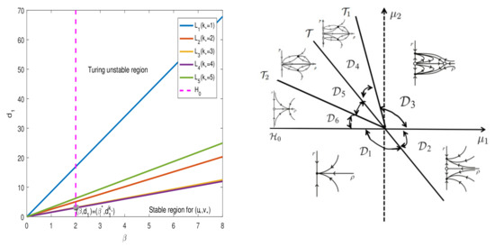
Figure 1. Left: some regions of $(u_{*},v_{*})$ and some curves in the $d_1-\beta$ plane. Right: the phase diagram, which is described more in Proposition 1.

Using (23), the normal form for system (25) at the Turing–Hopf bifurcation point can be calculated:

$$\left\{\begin{array}{cc}\hfill & {\dot{z}}_1=0.1029\left(1.0000{\mu }_1+1.0714{\mu }_2\right)z_1-2.1102z_1^3+2.2109z_1{z}_2{\overline{z}}_2,\hfill \\ \hfill & {\dot{z}}_2=0.4330i{z}_2+(0.0938+0.1083i){\mu }_1{z}_2+(-8.1018+2.2894i)z_1^2{z}_2-(2.0714+8.2719i)z_2^2{\overline{z}}_2,\hfill \\ \hfill & {\dot{\overline{z}}}_2=-0.4330i{\overline{z}}_2+(0.0938-0.1083i){\mu }_1{\overline{z}}_2+(-8.1018-2.2894i)z_1^2{\overline{z}}_2-(2.0714-8.2719i)z_2{\overline{z}}_2^2.\hfill \end{array}\right.$$

Using the same tranformation as (24), we obtain

$$\left\{\begin{array}{cc}\hfill & \dot{r}=0.1029\left(1.0000{\mu }_1+1.0714{\mu }_2\right)r-2.1102r^3+2.2109r{\rho }^2,\hfill \\ \hfill & \dot{\rho }=0.0938{\mu }_1\rho -8.1018\rho r^2-2.0714{\rho }^3.\hfill \end{array}\right.$$

(26)

From [21], considering $\rho >0$, system (26) has the following equilibria:

(1)

The coexistence equilibrium: $A_0=(0,0)$.

(2)

The spatially inhomogeneous steady states:

$$A_1^{\pm }=(\pm 0.0590\sqrt{14.0{\mu }_1+15.0{\mu }_2},0),for14.0{\mu }_1+15.0{\mu }_2>0.$$

(3)

The spatially homogeneous periodic solution:

$$A_2=(0,0.2123\sqrt{{\mu }_2}),for{\mu }_2>0.$$

(4)

The spatially inhomogeneous periodic solutions:

$$A_3^{\pm }=\left(\pm \sqrt{0.0096(1.0{\mu }_1+2.0434{\mu }_2)},\sqrt{-0.034\left(1.0{\mu }_1+0.8342{\mu }_2\right)}\right),$$

$$for1.0{\mu }_1+2.0434{\mu }_2>0and1.0{\mu }_1+0.8342{\mu }_2<0.$$

Through analysis of the existence of these equilibria for system (26), the following critical bifurcation curves are obtained:

$$\begin{array}{cc}\hfill {\mathcal{H}}_0:& {\mu }_2=0,\mathcal{T}:{\mu }_2=-0.9333{\mu }_1,\hfill \\ \hfill {\mathcal{T}}_1:& {\mu }_2=-1.1987{\mu }_1,{\mu }_1\le 0,{\mathcal{T}}_2:{\mu }_2=-0.4894{\mu }_1,{\mu }_1\le 0.\hfill \end{array}$$

(27)

These bifurcation curves, $\mathcal{T},{\mathcal{T}}_1$, and ${\mathcal{T}}_2$, divide the parameter plane $\left({\mu }_1,{\mu }_2\right)$ into six regions, see Figure 1 (Right). From each area, we gain Proposition 1:

Proposition 1.

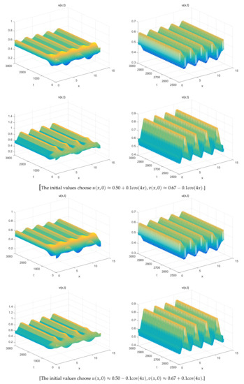
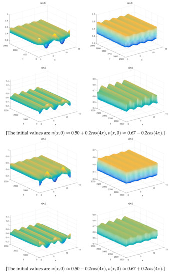
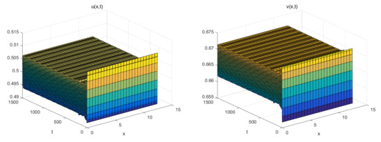
The Figure 1 (Right) shows more different dynamic phenomena by analyzing the stability of the equilibria of system (26). For each parameter region, we obtain some interesting results. When $\left({\mu }_1,{\mu }_2\right)\in D_1$, a coexistence equilibrium $A_0$, exists which is asymptotically stable (Figure 2). However, $A_0$ becomes unstable if $\left({\mu }_1,{\mu }_2\right)\notin D_1$. When $\left({\mu }_1,{\mu }_2\right)\in D_2$, a pair of spatially inhomogeneous steady states $A_1^{\pm }$ exist, along with an unstable coexistence equilibrium $A_0$, which is attracted by stable $A_1^{\pm }$ (Figure 3). When $\left({\mu }_1,{\mu }_2\right)\in D_3$, a pair of spatially inhomogeneous steady states $A_1^{\pm }$ remain stable, while a spatially homogeneous periodic solution $A_2$ becomes unstable (see Figure 4). When $\left({\mu }_1,{\mu }_2\right)\in D_4$, a pair of spatially inhomogeneous steady states $A_1^{\pm }$ and a spatially homogeneous periodic solution $A_2$ become unstable; however a pair of stable spatially inhomogeneous periodic solutions $A_3^{\pm }$ appears (see Figure 5). When $\left({\mu }_1,{\mu }_2\right)\in D_5$, a pair of spatially inhomogeneous steady states $A_1^{\pm }$ disappear, the stability of a pair of spatially inhomogeneous periodic solutions $A_3^{\pm }$ has not changed, and an unstable spatially homogeneous periodic solution $A_2$ tends toward stable $A_3^{\pm }$ (Figure 6). When $\left({\mu }_1,{\mu }_2\right)\in D_6$, there only a stable spatially homogeneous periodic solution $A_2$ exists, which means that the system (26) indicates temporal patterns (Figure 7).

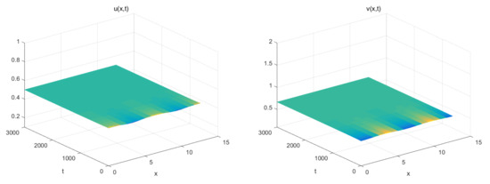
Figure 2. For $\left({\mu }_1,{\mu }_2\right)=\left(-0.1,-0.01\right)\in D_1$. Where $A_0$ is the coexistence equilibrium, which is asymptotically stable.

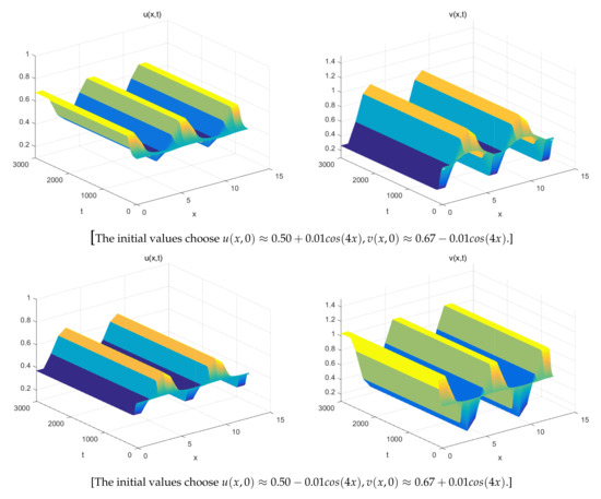
Figure 3. For $\left({\mu }_1,{\mu }_2\right)=\left(0.1,-0.01\right)\in D_2$, a pair of spatially inhomogeneous steady states $A_1^{\pm }$ exists, which is stable.

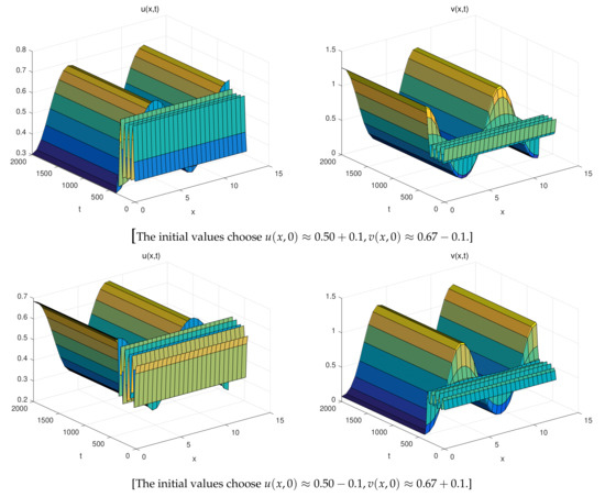
Figure 4. For $({\mu }_1,{\mu }_2)=(0.1,1.0)\in D_3$, $A_1^{\pm }$ (a pair of spatially inhomogeneous steady states) remains stable, but a track which connects with an unstable spatially homogeneous periodic solution $A_2$ exists.

Figure 5. When $({\mu }_1,{\mu }_2)=(-0.01,0.01)\in D_4$, there are three different types of solutions, a pair of spatially inhomogeneous periodic solutions $A_3^{\pm }$ remains stable, $A_1^{\pm }$ become unstable, and $A_2$ remains unstable in this region. A track connects them with each other.

Figure 6. For $\left({\mu }_1,{\mu }_2\right)=\left(-0.05,0.03\right)\in D_5$, $A_3^{\pm }$ (a pair of spatially inhomogeneous periodic solutions) remains stable, while $A_2$ becomes unstable and tends toward $A_3^{\pm }$.

Figure 7. The initial values are $u\left(x,0\right)\approx 0.50+0.01andv\left(x,0\right)\approx 0.67-0.01$. When $\left({\mu }_1,{\mu }_2\right)=\left(-0.4,0.1\right)\in D_6$, only a stable spatially homogeneous periodic solution $A_2$ exists.

6. Conclusions

Ryu et al. [15] have conducted much fantastic work to analyze model (3). From [22], we know that Turing instability may take place if diffusion terms are added to an ordinary differential equation system. In particular, we find that the system (4) with classical Holling I–III types can not occur during Turing instability (see Remark 1). Therefore, based on model (3), a diffusive predator–prey model with functional response (1) is considered in this article. From Theorem 2, we find that Turing instability could take place when Case 3 holds. Theorem 3 shows the conditions necessary for the existence of Hopf bifurcation. We used the central manifold and normal forms from [21] to explore whether Turing–Hopf bifurcation occurs. This is also the source of both the difficulty and novelty of our article. We chose $\beta ,d_1$ as bifurcation parameters and divided the bifurcation diagram into six regions. The model produced different states for each region. In $D_1$, it shows that the positive equilibrium of system (4) is asymptotically stable, which means two populations (predator and prey) will survive together and keep stable. In $D_2$, due to a pair of stable spatially inhomogeneous steady states (which means that the two populations (predator and prey) finally tend to being stable), the spatial distributions of populations are inhomogeneous. In $D_3$, a pair of spatially inhomogeneous steady states (which are stable) and a spatially homogeneous periodic solution (which is unstable) appear. This means that the two populations (predator and prey) will exhibit periodic oscillation and tend to be stable in the end. In $D_4$, there are three different types of solutions, a pair of spatially inhomogeneous periodic solutions ($A_3^{\pm }$) which are stable, and $A_1^{\pm }$ and $A_2$ which are unstable in this region. This means that the state of the two populations has been chaotic since the beginning, ultimately periodic phenomena may appear, which tend to stability. In $D_5$, a pair of spatially inhomogeneous steady states, $A_1^{\pm }$, became non-existent. This means that predator and prey will coexist and exhibit oscillatory behavior. In $D_6$, the system (4) only has a stable spatially homogeneous periodic solution. This also means that predator and prey will coexist and exhibit oscillatory behavior. Finally, the results of numerical simulations to support the above work which indicate the model (4) have more complex dynamic properties (see Figure 2, Figure 3, Figure 4, Figure 5, Figure 6 and Figure 7).

References

- Sabin, G.C.W.; Summers, D. Chaos in a periodically forced predator-prey ecosystem model. Math. Biosci. 1993, 113, 113. [Google Scholar] [CrossRef]
- Sadhu, S.; Kuehn, C. Stochastic mixed-mode oscillations in a three-species predator-prey model. Chaos 2018, 28, 033606. [Google Scholar] [CrossRef] [PubMed]
- Gilioli, G.; Pasquali, S.; Ruggeri, F. Nonlinear functional response parameter estimation in a stochastic predator-prey model. Math. Biosci. Eng. 2017, 9, 75–96. [Google Scholar]
- Shi, Q.; Shi, J.; Song, Y. Hopf bifurcation in a reaction-diffusion equation with distributed delay and Dirichlet boundary condition. J. Differ. Equ. 2017, 263, 6537–6575. [Google Scholar] [CrossRef]
- Bica, A.M.; Muresan, S. Smooth Dependence by LAG of the Solution of a Delay Integro-Differential Equation from Biomathematics. Commun. Math. Anal. 2006, 1, 64–74. [Google Scholar]
- Xiao, D.; Ruan, S. Multiple Bifurcations in a Delayed Predator-Prey System with Nonmonotonic Functional Response. J. Differ. Equ. 2001, 176, 494–510. [Google Scholar] [CrossRef] [Green Version]
- Lamontagne, Y.; Coutu, C.; Rousseau, C. Bifurcation analysis of a predator-prey system with generalised Holling type III functional response. J. Dyn. Differ. Equ. 2008, 20, 535–571. [Google Scholar] [CrossRef]
- Yang, R.; Ming, L.; Zhang, C. A delayed-diffusive predator-prey model with a ratio-dependent functional response. Commun. Nonlinear Sci. Numer. Simul. 2017, 53, S1007570417301508. [Google Scholar]
- Yang, R.; Zhang, C. Dynamics in a diffusive predator-prey system with a constant prey refuge and delay. Nonlinear Anal. Real World Appl. 2016, 31, 1–22. [Google Scholar] [CrossRef]
- Holling, C.S. The functional response of predators to prey density and its role in mimicry and population regulation. Mem. Entomol. Soc. Can. 1965, 97, 1–60. [Google Scholar] [CrossRef] [Green Version]
- Holling, C.S. Resilience and stability of ecological systems. Annu. Rev. Ecol. Syst. 1973, 4, 1–23. [Google Scholar] [CrossRef] [Green Version]
- Holling, C.S.; Sra, B. A behavioral model of predator-prey functional responses. Syst. Res. Behav. Sci. 2010, 21, 183–195. [Google Scholar] [CrossRef]
- Partridge, B.L.; Johansson, J.; Kalish, J. The structure of schools of giant bluefin tuna in Cape Cod Bay. Environ. Biol. Fishes 1983, 9, 253–262. [Google Scholar] [CrossRef]
- Cosner, C.; Deangelis, D.L.; Ault, J.S. Effects of spatial grouping on the functional response of predators. Theor. Popul. Biol. 1999, 56, 65–75. [Google Scholar] [CrossRef] [Green Version]
- Ryu, K.; Ko, W.; Haque, M. Bifurcation analysis in a predator-prey system with a functional response increasing in both predator and prey densities. Nonlinear Dyn. 2018, 94, 1639–1656. [Google Scholar] [CrossRef] [Green Version]
- Faria, T. Stability and bifurcation for a delayed predator-prey model and the effect of diffusion. J. Math. Anal. Appl. 2001, 254, 433–463. [Google Scholar] [CrossRef] [Green Version]
- Xu, Z.; Song, Y. Bifurcation analysis of a diffusive predator-prey system with a herd behavior and quadratic mortality. Math. Methods Appl. Sci. 2015, 38, 2994–3006. [Google Scholar] [CrossRef]
- Wolkowicz, G.S.K. Bifurcation analysis of a predator-prey system involving group defence. Siam J. Appl. Math. 1988, 48, 592–606. [Google Scholar] [CrossRef]
- Singh, M.K.; Bhadauria, B.S.; Singh, B.K. Bifurcation analysis of modified Leslie-Gower predator-prey model with double Allee effect. Ain Shams Eng. J. 2016, 9, S2090447916301095. [Google Scholar] [CrossRef] [Green Version]
- Song, Y.; Peng, Y.; Zhang, T. The spatially inhomogeneous Hopf bifurcation induced by memory delay in a memory-based diffusion system. J. Differ. Equ. 2021, 300, 597–624. [Google Scholar] [CrossRef]
- Jiang, W.; An, Q.; Shi, J. Formulation of the normal forms of Turing-Hopf bifurcation in reaction-diffusion systems with time delay. J. Differ. Equ. 2020, 268, 6067–6102. [Google Scholar] [CrossRef]
- Yi, F. Turing instability of the periodic solutions for reaction-diffusion systems with cross-diffusion and the patch model with cross-diffusion-like coupling. J. Differ. Equ. 2021, 281, 379–410. [Google Scholar] [CrossRef]
Publisher’s Note: MDPI stays neutral with regard to jurisdictional claims in published maps and institutional affiliations. |
© 2021 by the authors. Licensee MDPI, Basel, Switzerland. This article is an open access article distributed under the terms and conditions of the Creative Commons Attribution (CC BY) license (https://creativecommons.org/licenses/by/4.0/).