Abstract
This study presents LPV H∞ control with an augmented nonlinear observer (ANOB) to improve both the position and yaw tracking errors for Sawyer motors. The proposed control method consists of the forces and torque modulation scheme, an ANOB, and a Lyapunov-based current controller with the LPV H∞ state feedback controller to guarantee the stability of tracking error dynamics. The ANOB is designed to estimate all the state variables including the position, velocity, current, and disturbance using only position feedback. We propose a vertex expansion technique to solve the influence of the convex interpolation parameters in the LPV system on the tracking error performance. To be robust against disturbance, a state feedback controller with the LPV gain scheduling is determined by applying the H∞ control in the linear-matrix-inequality (LMI) technique. The closed-loop stability is proved through the Lyapunov theory. The effectiveness of the proposed control method is evaluated through simulation results and compared with the conventional proportional-integral-derivative (PID) control method to verify both the improved tracking error performance and a suitable disturbance rejection.
1. Introduction
In high-precision motion control, Sawyer motors have been widely used to achieve the strict requirements in position ControlThese motors play an extremely important role in automated assembly lines, precision machining tools, and semiconductor wafer stage systems. The Sawyer motors are dual-axis linear motors that have four forcers mounted symmetrically on the housing part [1]. Forcers X1 and X2 generate force in the X direction while forcers Y1 and Y2 generate force in the Y direction, as shown in Figure 1. Yaw of the motor is generated by asymmetries in the forcers and leads to loss of synchronization between the motor and platen teeth. The motor is not only a high-order dynamics but also has complex nonlinear properties. In addition, the motor has high position resolution and speed motion in the open-loop microstepping ControlHowever, it can have step-out, a long settling time, and especially low disturbance compensation. These problems are closely related to the yaw motion control that degrades the position tracking performance. Thus, the motor requires a highly accurate position control method.
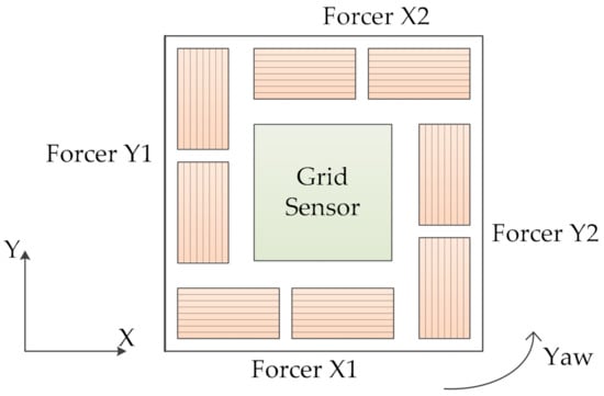
Figure 1.
Bottom view of a Sawyer motor.
Many advanced control approaches have been proposed to improve the position tracking performance for the Sawyer motors [1,2,3,4,5]. Structures of various robust adaptive controllers have been developed to guarantee position tracking performance [1,2]. To achieve the desired position, the nonlinear cascade control algorithms used linear techniques, such as conventional PID control [3]. By modifying proportional-integral-derivative (PID) and lead-and-PI compensators, they are designed to obtain the desired performances [4]. A combination of robust adaptive control and iterative learning control make compensation decisions to adapt to uncertain parameters and improve transient response in the position control [5]. However, the above-mentioned control algorithms are not optimal in the position tracking performance because the optimal control of nonlinear systems is very difficult and a great challenge. Although the optimal control of these motors was also studied to improve the positioning precision [6,7], the performance criteria for nonlinear dynamics are still uncertain and the influence of disturbance in the position control has not been considered; disturbance plays a critical role and directly affects control of the yaw angle of the motor. In addition, complex nonlinear models of the systems always contain nonlinear parameters that vary throughout the control process, making the nonlinear control system unstable. Therefore, linear parameter varying (LPV) systems whose nonlinear parameters are updated continuously online through measurements were developed to improve the control quality through greater stability and robustness [8,9,10].
To address the influence of disturbance, many different disturbance observers (DOBs) were designed to estimate and compensate for disturbance [11,12,13,14,15,16,17,18,19]. DOB was generalized to obtain the high-order disturbances in the sense of the time series expansion [11]. The use of all the measured states and linear DOB techniques based on control algorithms to reject external disturbance was studied in [12,13,14,15]. To improve the transient response by compensating for unknown and uncertain disturbances, a state-space DOB is proposed in [16,17]. However, the limitation of the aforementioned DOBs needs accurate state information regarding the nonlinear dynamics to estimate disturbance. This limitation is extremely difficult in practice to measure all the state variables using sensors because there are several problems, such as cost and space limitations. Therefore, an augmented nonlinear observer (ANOB) design is considered to estimate all the state variables including disturbance. In addition, there are different strategies to compensate the friction using the friction model and comparing the output of the inverse model and the input of the original nonlinear system [18,19]; however, it is difficult for friction compensation because the friction is very diverse. In the context of the previous studies mentioned above, the augmented nonlinear observer design is essential for the Sawyer motors to improve the transient response in position control in the presence of disturbance.
The main contribution of this study was to design the LPV H∞ control with an ANOB to reduce both the position and yaw tracking errors for the Sawyer motors in the presence of disturbance. The proposed control method consists of the forces and torque modulation scheme, an ANOB, and a Lyapunov-based current controller with the LPV H∞ state feedback controller. The forces and torque modulation scheme is developed to guarantee the stability of the position and yaw tracking errors for the mechanical tracking error dynamics and to generate the desired phase currents. A Lyapunov-based current controller with an LPV H∞ state feedback controller is proposed to guarantee the stability of phase current tracking errors for the electrical tracking error dynamics under the influence of back-electromotive forces (EMFs) and phase lag by inductances during operation. All the state variables (position, velocity, current) including the load forces and load torque are estimated by using only the position feedback. Estimated state variables are used instead of the measured signals. This makes the control performance unaffected under the measurement noise in the currents. The position control problem of the Sawyer motor was analyzed in the optimal LPV problem. A vertex expansion technique is introduced to compute the convex interpolation parameters to solve the influence of vertices on the tracking performance in the LPV system. To be robust against disturbance, a state feedback controller with the LPV gain scheduling is determined by applying the H∞ control in the linear-matrix-inequality (LMI) technique. The closed-loop stability is proved through the Lyapunov theory. The effectiveness of the proposed control method was demonstrated by comparing the simulation results with the performance of the conventional PID control method.
This article is organized into seven sections. Section 2 describes the mathematical model of the Sawyer motor. Section 3 defines the forces, torque modulation scheme, and the Lyapunov-based current controller. Section 4 defines the configuration of the LPV system. Section 5 proposes the ANOB and H∞ feedback control design using LPV synthesis including the ANOB and LPV H∞ state feedback ControlSection 6 presents the simulation results of the proposed control method and a performance comparison with the conventional PID control method. Finally, Section 7 presents the conclusions.
2. Mathematical Model of Sawyer Motor
The mathematical model of the Sawyer motor consists of mechanical and electrical dynamics that can be respectively represented [1,2] as follows:
where and
where , , and are the positions of the X-axis, Y-axis, and yaw rotation of the motor, respectively; , , and are the velocities of the X-axis, Y-axis, and yaw rate of the motor, respectively; and are the distances from the center of the motor to the forcer; and are forces made by the two X-axis forcers, whereas and are forces made by the two Y-axis forcers; is the force constant; and denote the motor mass and inertia, respectively; , , and are coefficients of friction; is the tooth pitch of the platen; , , , , , , , and are phase currents; , , , , , , , and are input voltages in phases A and B; and , , and are unknown load forces and torque, respectively.
3. Forces, Torque Modulation Scheme, and Lyapunov-Based Current Controller
3.1. Tracking Error Dynamics
Let us define the tracking-error state vectors as follows:
where:
where , , and are the desired positions of the X-axis, Y-axis, and yaw rotation, respectively; , , and are the virtual velocities of the X-axis, Y-axis, and virtual yaw rate, respectively; , , and are the position tracking errors of the X-axis, Y-axis, and yaw rotation, respectively; , , and are the velocity tracking errors of the X-axis, Y-axis, and yaw rate, respectively; , , , , , , , and are the desired phase currents; and , , , , , , , and are the current tracking errors in phases A and B.
Differentiating (5) with respect to time, the tracking error dynamics are represented as follows:
where , , and .
3.2. Forces and Torque Modulation Scheme
To guarantee the stability of the position and yaw tracking errors for the mechanical tracking error dynamics, we propose to express the forces and torque modulation in the LPV system as follows:
where , , , , , and are positive constants.
We define the commutation scheme in the LPV system to generate the desired phase currents as follows:
3.3. Lyapunov-Based Current Controller
To guarantee the stability of phase current tracking errors for the electrical tracking error dynamics under the influence of back-EMFs and phase lag by inductances during operation, we propose the Lyapunov-based current controller with LPV H∞ state feedback control in the LPV system in terms of Theorem 1.
Theorem 1.
According to the tracking error dynamics expressed by (6) and (7), the voltage inputs of the Sawyer motor are defined as follows:
where the H∞ state feedback control law with LPV gain schedulingfor the electrical tracking error dynamics, whose design is presented in
Section 5, is expressed as follows:
Proof of Theorem 1.
Let us consider the first Lyapunov function candidate:
The derivative of with respect to time is expressed as follows:
Let us consider now the second Lyapunov function candidate:
Using (8), the derivative of with respect to time is obtained as follows:
Let us finally consider the third Lyapunov function candidate:
Using , , , , , , , and in (12), and the LPV H∞ state feedback control law with LPV gain scheduling given by (13), the derivative of with respect to time is obtained as follows:
Let us introduce the following definition:
where and
According to the Schur complement [20], is equivalent to the following expression:
Given that , and always exists to satisfy the condition in (18), is definitely negative. Therefore, converges to zero and the closed-loop stability is guaranteed.
Substituting (9), (10), (11), and (12) into (6) and (7), the tracking error dynamics can be re-written as follows:
□
4. Configuration of LPV System
4.1. LPV System
The varying parameters of the tracking error dynamics are defined as follows:
Given that these are trigonometric functions, the varying parameters are bounded as follows:
where .
Therefore, the tracking error dynamics of the Sawyer motor expressed in (19) and (20) can be transformed into an LPV system expressed as follows:
The parameter-dependent matrix and are defined as follows:
where , , ,
The varying parameters , , , , ,, , and can be continuously updated online during the control process through the measurements of , , , and . Moreover, the values of these varying parameters are limited by known upper and lower bounds, as expressed in (22). These varying parameters can be described as polytopic:
where is a convex interpolation parameter vector, is a vertex, and satisfying the following conditions:
Therefore, determined in the LPV system through (23) can be expressed as follows:
where , , and .
We define the polytopic decomposition as follows:
where and are real-fixed nodal matrices related to and extreme values of the varying parameters.
4.2. Vertex Expansion Technique
The convex interpolation parameter vector plays an important role in determining the parameter-dependent matrix . It is computed based on vertices. Given that the vertex V cannot implement the inverse, we propose the vertex expansion technique through Definition 1:
Definition 1.
Considerandwe define, andas the constrained polytopic parameters. If , then we have the following expressions:
According to Definition 1 and the varying parameters limited by known upper and lower bounds, as expressed in (22), . We have extended the V vertex to satisfy the inverse. Thus, the varying parameter vector is expressed as follows:
Finally, the convex interpolation parameter vector is computed as follows:
The vertices must simultaneously comply with the following constraint conditions:
5. Augmented Nonlinear Observer and H∞ Feedback Control Design Using LPV Synthesis
5.1. Augmented Nonlinear Observer
In the previous section, we assumed that all the state variables are measurable in the error dynamics, LPV system, and the proposed current controller. The measurement of all the state variables is extremely difficult by using sensors because there are several problems, such as cost and space limitations. In addition, to be robust against disturbance in the position control, the load forces and torque as disturbance must be determined. This subsection describes the design of an augmented nonlinear observer by using only position feedback to obtain all the state variables (position, velocity, current) including disturbance. In practice, the load forces and torque vary very slowly; therefore, it can be reasonably supposed that , , and, . The augmented nonlinear observer is designed as follows:
where
Let us define the vector , the estimation vector , and the estimation error vector of the augmented state variables as follows:
and
where
and
The estimation error dynamics of the augmented state variables can be given as follows:
where , , and
Theorem 2.
Consider the estimation error dynamics of the augmented state variables (38). If an observer gain matrix L can be chosen such that:
whereandis the maximum eigenvalue of. Then, exponentially converges to zero.
Proof of Theorem 2.
Let us consider the Lyapunov function candidate:
The derivative of with respect to time is expressed as follows:
Thus, if , then exponentially converges to zero [21]. □
Remark 1:
Since the proposed method guarantees the exponential stability of the zero equilibrium point of (39), the proposed method guarantees the robustness against the parameter uncertainties if the parameter uncertainties can be regarded as the vanishing perturbation term [21]. However, if the parameter uncertainties are in the form of the nonvanishing perturbation term, the proposed method guarantees only the boundedness of the tracking error and the estimation error [21].
5.2. LPV H∞ State Feedback Control and Closed-Loop Stability Analysis
In the previous subsection, we discussed the augmented nonlinear observer design to obtain all the state variables (position, velocity, current) including the load forces and torque as disturbance. In this subsection, we present the design of the pre-defined control inputs , , , , , , , and in the context of a linear system using H∞ optimization. The estimated state variables are used instead of the measured signals so that the control performance is not affected by the measurement noise. Let us define the tracking-error state vectors of the augmented state variables as follows:
From (23), the tracking error dynamics in the LPV system becomes:
where is the objective function signal, is as the exogenous disturbance signal, is the covariance matrix, and and are the weighting matrices of the tracking errors and control inputs, respectively:
The LPV H∞ state feedback control law becomes as follows:
where is the LPV gain scheduling.
The closed-loop system dynamics of the proposed control method is illustrated in Figure 2. The state vectors are defined as follows:
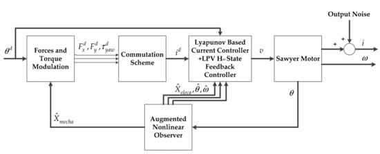
Figure 2.
Structure of the proposed control method.
The stability of the closed-loop system dynamics consists of the estimation error dynamics of the augmented state variables (38) and tracking errors dynamics (41) as follows:
Theorem 3.
Consider the closed-loop system dynamics (43). If the LPV gain scheduling and observer gain matrix L can be chosen such that:
whereandis the maximum eigenvalue of. Then, exponentially converges to zero.
Proof of Theorem 3.
Let us consider the Lyapunov function candidate:
The derivative of with respect to time is expressed as follows:
Thus, if , then exponentially converges to zero [21]. □
To determine the LPV gain scheduling , we apply the H∞ control in the LMI technique with Assumption 1 in the optimal control design [22]:
Assumption 1.
- (A1)
- is stable.
- (A2)
- is invertible.
- (A3)
- .
- (A4)
- has no unobservable modes on the imaginary axis.
Note that the H∞ norm of the LPV control system is represented as follows:
The LPV H∞ state feedback control will determine the bound on the H∞ norm of the LPV control system with the linear matrix inequality (LMI) condition. The following statements are equivalent.
- There exists such that .
- There exists such that:
Given that we design the H∞ state feedback control based on the LPV system, is interpolated by the polytopic decomposition . Therefore, the linear matrix inequality given by (46) is redefined as follows:
Then, we define a new variable as , so the LPV gain scheduling of the state feedback control is recovered by with the following LMI condition:
Finally, the LPV H∞ state feedback control law is expressed as follows:
6. Simulation Results
We utilized the Sawyer motor parameters, control gains, and augmented nonlinear observer gains listed in Table 1. The desired position profiles were those of the ramp function as shown in Figure 3, and the yaw desired profile was set to 0 rad.

Table 1.
Sawyer motor parameters, control gains, and augmented nonlinear observer gains.
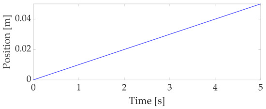
Figure 3.
X-axis and Y-axis desired position profiles.
The results of the 16 interpolation parameters are shown in Figure 4 to satisfy the constraint conditions related to the proposed vertex expansion technique in Section 4. The maximum value of each interpolation parameter is 0.125, in which the influence of the load forces and torque as exogenous disturbance of the X-axis, Y-axis, and yaw at 2 s is shown in Figure 5. From these results, we confirm that the proposed LPV control system performs well.
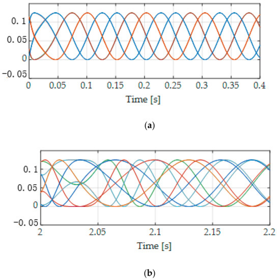
Figure 4.
Sixteen interpolation parameters of the LPV control system. (a) Zoom-in X-axis at the start time of 16 interpolation parameters. (b) Zoom-in X-axis at 2 s of 16 interpolation parameters.
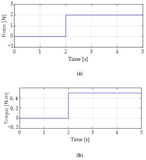
Figure 5.
Load forces and load torque. (a) Load forces and (b) Load torque .
The estimation performance of the proposed ANOB of positions of the X-axis, Y-axis, yaw rotation, the load forces and torque, and phase currents is confirmed as shown in Figure 6. In addition, the estimation error performance is also represented in Figure 7. We verify that the load forces and torque and the state variables were well estimated by applying the proposed ANOB in the presence of 5% output noise of the current.
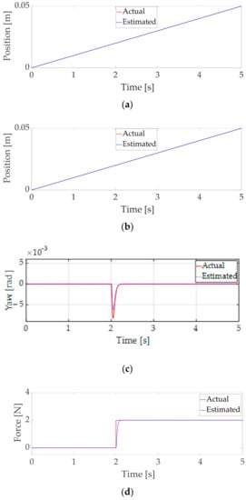
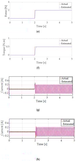
Figure 6.
Estimation performance of the proposed ANOB. (a) Estimation performance of and . (b) Estimation performance of and . (c) Estimation performance of and . (d) Estimation performance of and . (e) Estimation performance of and . (f) Estimation performance of and . (g) Estimation performance of and . (h) Estimation performance of and .
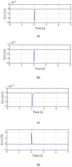
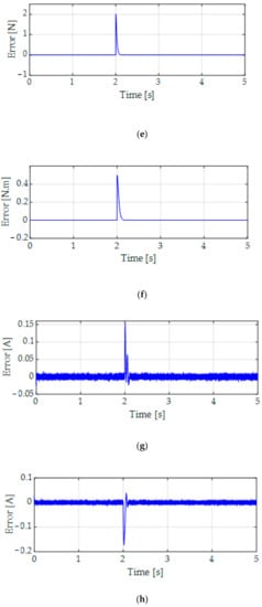
Figure 7.
Estimation error performance of the proposed ANOB. (a) Estimation error performance of . (b) Estimation error performance of . (c) Estimation error performance of . (d) Estimation error performance of . (e) Estimation error performance of . (f) Estimation error performance of . (g) Estimation error performance of . (h) Estimation error performance of .
To evaluate the effectiveness of the proposed control method in the influence of the load forces and torque as exogenous disturbance, output noise as well as the robustness to uncertain parameters by 5% change of the nominal parameters including inertia and coefficients of friction , and of the motor, we represented the simulation results in the following two cases:
Case 1: Conventional PID control.
Case 2: LPV H∞ control with an ANOB.
The position and yaw tracking errors of the two cases are shown in Figure 8. Note that the conventional PID control in Case 1 had a large overshoot during the acceleration and the deceleration periods as well as violent oscillations of yaw motion. The effect of controller gains in Case 1 was high for tracking error dynamics, which means a long settling time in the transient response for the position and yaw tracking error control.
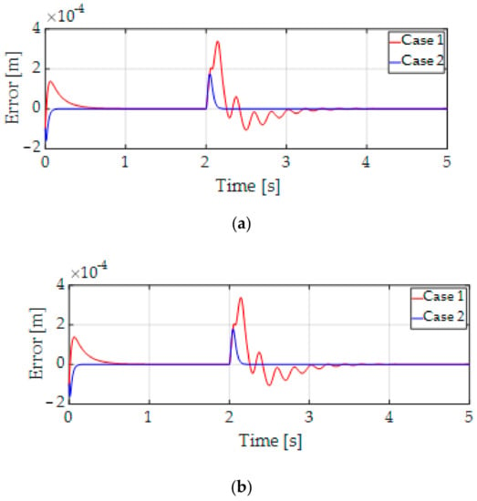
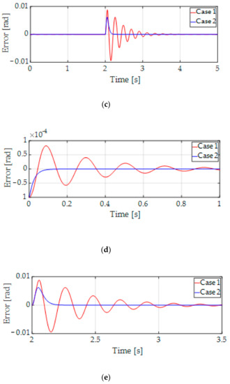
Figure 8.
Position and yaw tracking errors. (a) X-axis position tracking error of . (b) Y-axis position tracking error of . (c) Yaw tracking error of . (d) Zoom-in X-axis at the start time of . (e) Zoom-in X-axis at 2 s of .
In Case 2, the position and yaw tracking errors were improved, and the oscillation of yaw motion was considerably reduced in the proposed control method because the LPV gain scheduling was controlled to regulate the tracking errors. The convergences of position and yaw tracking errors are zero. Figure 8 also shows that the yaw motion is well regulated in the influence of the load forces and torque as exogenous disturbance at 2 s and uncertain parameters because the effectiveness of the H∞ control was guaranteed by using the H∞ norm in (45) to be robust against disturbance. We confirm that the proposed control method improves the tracking error performance and rejects disturbance better than the conventional PID control method.
7. Conclusions
This study proposes LPV H∞ control with an augmented nonlinear observer for the Sawyer motors. The proposed control method consists of the forces and torque modulation scheme, the augmented nonlinear observer, and the Lyapunov-based current controller with the LPV H∞ state feedback controller to reduce the tracking error dynamics. The forces and torque modulation scheme is developed to guarantee the stability of the position and yaw tracking errors for the mechanical tracking error dynamics and to generate the desired phase currents. The augmented nonlinear observer is designed to estimate all the state variables including disturbance using only the position feedback. The Lyapunov-based current controller with an LPV H∞ state feedback controller is proposed to guarantee the stability of phase current tracking errors for the electrical tracking error dynamics. The effectiveness of the proposed control method was verified through simulation results and compared with the conventional PID control method, showing improved tracking error performance and suitable disturbance rejection.
One possible future research direction is to consider polytopic representation of the LPV system using the tensor product approach to derive a polytopic convex model with various convex hull representations [23,24,25].
Author Contributions
K.H.S. and K.B. designed the algorithm and developed the simulation; Y.L. and W.K. provided guidance in designing the algorithm. All authors have read and agreed to the published version of the manuscript.
Funding
This study was financially supported by the Chung-Ang University Research Scholarship Grants in 2021 and partly by Basic Science Research Program through the National Research Foundation of Korea (NRF) funded by the Ministry of Education (2020R1I1A3073378).
Institutional Review Board Statement
Not applicable.
Informed Consent Statement
Not applicable.
Conflicts of Interest
The authors declare that they have no conflict of interest.
Abbreviations
| LPV | Linear parameter varying |
| ANOB | Augmented nonlinear observer |
| LMI | Linear matrix inequality |
| PID | Proportional integral derivative |
| DOB | Disturbance observer |
| EMF | Electromotive force |
References
- Krishnamurthy, P.; Khorrami, F. Robust adaptive control of Sawyer motors without current measurements. IEEE/ASME Trans. Mechatron. 2004, 9, 689–696. [Google Scholar] [CrossRef]
- Krishnamurthy, P.; Khorrami, F.; Ng, T.L.; Cherepinsky, I. Control design and implementation for Sawyer motors used in manufacturing systems. IEEE Trans. Control Syst. Technol. 2011, 19, 1467–1478. [Google Scholar] [CrossRef]
- Pan, J.; Cheung, N.C.; Yang, J. High-precision position control of a novel planar switched reluctance motor. IEEE Trans. Ind. Electron. 2005, 52, 1644–1652. [Google Scholar] [CrossRef]
- Nguyen, V.H.; Kim, W.J. Design and control of a compact light-weight planar positioner moving over a concentrated-field magnet matrix. IEEE/ASME Trans. Mechatron. 2013, 18, 1090–1099. [Google Scholar] [CrossRef]
- Hu, C.; Wang, Z.; Zhu, Y.; Zhang, M.; Liu, H. Performance-oriented precision LARC tracking motion control of a magnetically levitated planar motor with comparative experiments. IEEE Trans. Ind. Electron. 2016, 63, 5763–5773. [Google Scholar] [CrossRef]
- Huang, S.D.; Chen, L.; Cao, G.Z.; Wu, C.; Xu, J.; He, Z. Predictive position control of planar motors using trajectory gradient soft constraint with attenuation coefficients in the weighting matrix. IEEE Trans. Ind. Electron. 2021, 68, 821–837. [Google Scholar] [CrossRef]
- Huang, S.D.; Cao, G.Z.; Xu, J.; Cui, Y.; Wu, C.; He, J. Predictive position control of long-stroke planar motors for high-precision positioning applications. IEEE Trans. Ind. Electron. 2021, 68, 796–811. [Google Scholar] [CrossRef]
- Apkarian, P.; Gahinet, P.; Becker, G. Self-scheduled H∞ control of linear parameter-varying systems: A design example. Automatica 1995, 31, 1251–1261. [Google Scholar] [CrossRef]
- Packard, A. Gain scheduling via linear fractional transformations. Syst. Control Lett. 1994, 22, 79–92. [Google Scholar] [CrossRef]
- Shamma, S. Analysis and Design of Gain Scheduled Control Systems. Ph.D. Thesis, Massachusetts Institute of Technology, Cambridge, MA, USA, 1988. [Google Scholar]
- Kim, K.S.; Rew, K.H.; Kim, S. Disturbance observer for estimating higher order disturbances in time series expansion. IEEE Trans. Automat. Contr. 2010, 55, 1905–1911. [Google Scholar]
- Ishikawa, J.; Tomizuka, M. Pivot friction compensation using an accelerometer and a disturbance observer for hard disk drives. IEEE/ASME Trans. Mechatron. 1998, 3, 194–201. [Google Scholar] [CrossRef]
- Kim, K.H.; Youn, M.J. A nonlinear speed control for a PM synchronous motor using a simple disturbance estimation technique. IEEE Trans. Ind. Electron. 2002, 49, 524–535. [Google Scholar]
- Liu, H.; Li, S. Speed control for PMSM servo system using predictive functional control and extended state observer. IEEE Trans. Ind. Electron. 2012, 59, 1171–1183. [Google Scholar] [CrossRef]
- Cho, K.; Kim, J.; Choi, S.B.; Oh, S. A high-precision motion control based on a periodic adaptive disturbance observer in a PMLSM. IEEE/ASME Trans. Mechatron. 2015, 20, 2158–2171. [Google Scholar] [CrossRef]
- Lee, S.H.; Kang, H.J.; Chung, C.C. Robust fast seek control of a servo track writer using a state space disturbance observer. IEEE Trans. Control Syst. Technol. 2012, 20, 346–355. [Google Scholar] [CrossRef]
- Kang, H.J.; Kim, K.S.; Lee, S.H.; Chung, C.C. Bias compensation for fast servo track writer seek Control. IEEE Trans. Magn. 2011, 47, 1937–1943. [Google Scholar] [CrossRef]
- Delibas, B.; Koc, B. A method to realize low velocity movability and eliminate friction induced noise in piezoelectric ultrasonic motors. IEEE/ASME Trans. Mechatron. 2020, 25, 2677–2687. [Google Scholar] [CrossRef]
- Ding, S.; Chen, W.H.; Mei, K.; Murray-Smith, D.J. Disturbance observer design for nonlinear systems represented by input-output models. IEEE Trans. Ind. Electron. 2020, 67, 1222–1232. [Google Scholar] [CrossRef] [Green Version]
- Boyd, S.; Vandenberghe, L. Convex Optimization; Cambridge University Press: Cambridge, UK, 2003. [Google Scholar]
- Khalil, H.K. Nonlinear Systems, 3rd ed.; Prentice-Hall: Englewood Cliffs, NJ, USA, 2002. [Google Scholar]
- Lee, Y.W.; Lee, S.H.; Chung, C.C. LPV H∞ Control with disturbance estimation for permanent magnet synchronous motors. IEEE Trans. Ind. Electron. 2018, 65, 488–497. [Google Scholar] [CrossRef]
- Baranyi, P.; Yam, Y.; Varlaki, P. Tensor Product Model Transformation in Polytopic Model-Based Control; CRC Press: Boca Raton, FL, USA, 2013. [Google Scholar]
- Szollosi, A.; Baranyi, P. Influence of the tensor product model representation of qLPV models on the feasibility of linear matrix inequality. Asian J. Control 2016, 18, 1328–1342. [Google Scholar] [CrossRef]
- Takarics, B.; Vanek, B. Robust control design for the FLEXOP demonstrator aircraft via tensor product models. Asian J. Control 2021, 23, 1290–1300. [Google Scholar] [CrossRef]
Publisher’s Note: MDPI stays neutral with regard to jurisdictional claims in published maps and institutional affiliations. |
© 2021 by the authors. Licensee MDPI, Basel, Switzerland. This article is an open access article distributed under the terms and conditions of the Creative Commons Attribution (CC BY) license (https://creativecommons.org/licenses/by/4.0/).