Trade and Permanent Growth with Domestic and Foreign Capital Goods, and International Capital Movements

Abstract

Domestic and foreign capital and consumption goods are imperfect substitutes in production and demand functions of the growth model by Bardhan–Lewis. We extend the model by introducing exogenous technical progress and allow for foreign debt dynamics without dropping domestic capital goods. Trade and growth are mutually affecting each other. Trade may speed up or decrease growth in theory with and without technical progress in comparison with the Solow–Swan model. Steady-state growth rates include that of world income, and the income and price elasticities of export demand. The dynamic process of the economy is analyzed in terms of exports and foreign debt, and both as a share of a stock of imported capital goods. There are multiple steady states where imported capital goods are paid for by high exports and debt, low debt and low exports, or even negative debt and low exports. A stable VAR with data for Brazil shows that the high-debt steady state is relevant for this country. Steady states with high and low debt are saddle-point stable and the steady-state medium debt is stable. Neoclassical standard results appear as two special cases. We link the model to several strands of literature.

1. Introduction

According to economic theory there are three main links explaining how international trade affects growth. First, in static trade models, going from more to less restricted trade in the basic case of normal goods, there is more consumption and production of all goods and a higher utility level. Higher utility is associated with more income. Getting from lower to higher income is a process of comparative static growth, which, however, is not permanent but rather transitional. An open economy getting more of one factor, for example, labour through migration, leads to a larger production possibility set and, in case of limited effects on the terms of trade, to a higher level of production, income and consumption.

Second, in models of endogenous growth there are two effects under imperfect specialization. (i) Trade liberalization generates a larger market for intermediate goods, and if these are productive in R&D, as in the lab-equipment model of Rivera-Batiz and Romer (1991), the rate of technical progress increases. (ii) Suppose there are two factors of production, high and low skilled labour, and three sectors, with different skill intensities, one of which produces a non-tradable rate of technical progress; then trade leads to specialization in the good, which is relatively high (low)-skill intensive, thus competing skilled labour away from (into) the technical progress sector (Grossman & Helpman, 1991, Chapter 6). Technical progress will decrease (increase) through trade depending on the shift in production factors away from or to the activity producing technical change. The composition of these two effects will determine the impact of trade on endogenous growth. Several variations to these effects exist. There is no impact of income elasticities of export demand other than unity, because imported intermediates are working through CES functions. Consequently, technical change is the only driver of productivity, and there is no impact of a second driving force, world GDP growth, as in our model explained below.

Third, if in the previous example the economy under autarky does not produce technical progress, it may start doing so under trade if it specializes in the low-skill intensive goods and if this makes high-skill labour sufficiently cheap through the reduction in production in the high-skill intensive sector (Rivera-Batiz & Xie, 1993).

The latter two models have innovation-related trade channels. The downside of these three stories is that without technical change there can be no permanent growth under decreasing returns to reproducible factors.1 There are exceptions to these models. Imagine a simple Solow growth model. Next, assume that capital consists of goods, which are different from output, and all (merely for simplification) changes in the capital stock must be imported. Therefore, they must be paid for by exports, either now or later if foreign debt can be incurred. If there is an export demand function, where the quantity depends on the endogenous terms of trade and world income, the economy has two motors of growth: technical progress as in Solow’s model, if it is positive, and also world income (growth) in the export (growth) function.2 Growing world income may lead to permanent growth even if there is no technical progress. It allows earning foreign exchange, which can be used to import capital goods. If the product of world income growth and its income elasticity in the export function is larger than population growth, the economy grows permanently unless the small country assumption applies.3 The basic paper showing this is that of Bardhan and Lewis (1970), which contains also the domestic capital stock in a Cobb–Douglas function as in the Solow–Swan model. They consider it as a neoclassical version of two-gap theory. It is a trade channel related to capital accumulation. Ziesemer (1998) has related a simplified version of the model to the Prebisch–Singer thesis and to vent-for-surplus theory. Ziesemer (1995b) has added perfect capital movements and related the model to the issue of the link between exports and labour productivity, which consists of imported capital goods. The two mentioned papers did work with the simplifying assumption of having no domestic capital goods, which is abandoned in this paper.4 Whereas the role of income elasticities of demand is widely acknowledged in the literature (see Boppart, 2014, footnote 3), the unique feature of the literature just mentioned is that it combines the income elasticity and a finite export price elasticity with the fact of importing capital goods, which are imperfect substitutes in a Cobb–Douglas function, which has elasticity of substitution unity. Through this combination the steady-state growth rate includes world income and the income and price elasticities of export demand.

In this paper, we bring back domestic capital goods and emphasize the effect of trade for permanent growth through imported capital goods. We extend the Bardhan–Lewis model to introduce exogenous technical progress, and allow for foreign debt, without dropping domestic capital goods as in Ziesemer (1995b, 1998). Whereas in the neoclassical Solow–Swan model a country produces one good, which is used for consumption and capital formation, in our model each of two countries produces one good that is used for consumption and capital formation in both countries. Through imported capital goods trade and growth interact as in Bardhan and Lewis (1970). Adding technical change and foreign debt to the Bardhan/Lewis model produces several new interactions. The model has gained relevance from the recent development in Germany, a country that is strong in exports and in machinery and transport equipment (SITC 7). Germany has noticed recently that the diversification of the past has become less relevant compared to dependence on imported batteries, chips (with low nanometers like Intel’s 1.5; the cluster in Dresden has 12 to 28 nanometers), and digital machines, products and components. Imported inputs gain in relevance for a strong machine exporter.

The modified structure of the model responds to the overarching research question ‘what is the dynamic system of the model with foreign debt and domestic and foreign capital goods that replaces the central differential equation in one capital good in the Solow model and the system of two capital goods in the Bardhan–Lewis model?’. The answer is that there are multiple steady states for a dynamic system in debt and exports both expressed as percentage of the stock of foreign capital goods, where imported capital goods are paid for by high exports and debt, low debt and low exports, or negative debt and very low exports.5 For the perspective of the interaction of these three variables, the model by Bardhan and Lewis (1970) is the one that is most similar because in includes domestic and foreign capital goods, though not foreign debt. The model versions leaving out domestic capital goods induce the question whether less favourable growth results, if suggested by these models, could be avoided by substituting foreign capital goods by using more domestic capital goods, for example, in the case of falling terms of trade suggested by Prebisch (1950) and Singer (1999). This type of question can only be answered when both types of capital goods are included in the model. The following new results come from this paper’s model. We show that trade may speed up or decrease growth in theory with and without technical progress in comparison with the Solow model, and some results hold with and without production and use of domestic capital. However, through the introduction of domestic capital goods, there are not two regimes anymore as in Ziesemer (1995b). The Solow–Swan results as well as those associated with Prebisch (1950, 1959) and Singer (1999) are special cases of the model with and without technical change. Adding an empirical vector autoregressive (VAR) model in the debt and export ratios allows us to determine which of the steady states is most realistic for the country considered. We do this for data from Brazil.

Section 2 extends the Bardhan and Lewis (1970) model through foreign debt and technical change, and those of Ziesemer (1995a/1998, 1995b, 1998) by domestic capital goods. Section 3 provides a steady-state solution in growth rates, defines a steady state, shows non-uniqueness and (saddle-point) stability, derives comparative static results, estimates a VAR for Brazil in the variables of the theoretical model, and simulates forward to see where debt and export ratios go. Section 4 has a broad comparison with the literature. Section 5 provides a compact, non-technical summary and concludes.

2. Methodology: The Model

We start by making assumptions on technology, endowments, and preferences. Output, Y, is assumed to be produced by domestic capital, K_id, foreign capital, K_f, and labour, L, in a macroeconomic production function of the Cobb–Douglas type with total factor productivity b^et (uppercase letters depend on time t, but this is not written down explicitly):

$$Y=e^{bt}{K}_d^{\alpha }{K}_f^{\beta }{L}^{1-\alpha -\beta }$$

(1)

As this is a Cobb–Douglas function, the elasticity of substitution between any two factors is unity, in particular for domestic and foreign capital goods, and therefore they are all imperfect substitutes. This simplifying assumption excludes from the consideration the very low elasticities of substitution, which reduce the effects of price changes, and the very high ones, which possibly lead to non-existence of steady states (Harris, 1975).6 If domestic capital goods consist of units of domestic output, which has price P_d, whereas foreign capital goods have price P_f, nominal profits can be written as follows:

$$P_d{e}^{bt}{K}_d^{\alpha }{K}_f^{\beta }{L}^{1-\alpha -\beta }-\left(r+\delta \right)P_d{K}_d-\left(r+\delta \right)P_f{K}_f-WL$$

(2)

Costs are calculated at the corresponding credit costs at a given and constant world market interest rate r plus depreciation at rate δ. Marginal productivity conditions of profit maximizing choice of the inputs are derived as follows:

$$r+\delta ={\displaystyle \frac{\alpha Y}{K_d}}$$

(3)

$$r+\delta ={\displaystyle \frac{p\beta Y}{K_f}}, p\equiv {\displaystyle \frac{P_d}{P_f}}$$

(4)

$$w\equiv {\displaystyle \frac{W}{P_d}}=(1-\alpha -\beta )Y/L$$

(5)

We assume absence of rigidities for investment and no large shocks. Then the choice of investment into the capital stocks can always ensure marginal products of capital equal to capital costs, and the ensuing full-employment output determines wages. Conversely, for any given wage, employment/output ratios are chosen and wages are assumed to fall until this ensures full employment. Unemployment issues are not of interest in this paper.7 The second equation in (4) defines the terms of trade. There is an exogenous employment:

$$L=L_0{e}^{\epsilon t}$$

(6)

Gross investment, consisting of foreign and domestic capital goods, can be financed by domestic savings, S, or by a change (indicated by a dot) in foreign debt, D:

$${\dot{K}}_f+\delta K_f+p({\dot{K}}_d+\delta K_d)=S+\dot{D}$$

(7)

Equation (7) is formulated in units of foreign capital goods.8

Gross national income (GNI) is pY − rD. A share s of it is saved.9 Savings, S, are assumed to be a fixed percentage, s, of the value of output after interest has been paid:

$$S=s(pY-rD)$$

(8)

The change in the stock of foreign capital goods plus re-investment is imported, and other imports are a constant share γ of consumption, γ(1 − s)(pY − rD):10

$${M=\gamma \left(1-s\right)\left(pY-rD\right)+\dot{K}}_f+\delta K_f$$

(9)

Changes in debt are the result of the trade deficit and interest payments:

$$\dot{D}=M-pX+rD$$

(10)

Foreign debt allows paying for imported capital and consumption goods with exports later and consuming earlier. This comes at the cost of paying interest. Given the trade balance, the interest rate causes a partial instability: more interest payments lead to more new debt flows, which then lead to higher interest. If debt is increasingly negative, more consumption later is possible, and interest income may be an increasing share of GNI (Amano, 1965). The quantity of exports, X, is a function of world income, Z, with income elasticity, ρ, and the terms of trade, p, with price elasticity, η, which has a negative value:

$$X=Z^{\rho } p^{\eta }\equiv e^{\omega t}{p}^{\eta }, \omega \equiv \rho \widehat{Z}$$

(11)

The exponential formulation on the right-hand side of the second equation was used by Bardhan and Lewis (1970) and earlier by Johnson (1953) with p = 1. Using world income instead makes it possible to link the model to the literature emphasizing income elasticities of demand, here the exponent of Z.

Some simplifying assumptions made here like constant interest rates and constant population growth can be interpreted as rigidities. We do not impose other rigidities because we do not have the idea that they would change our results essentially. One well-known exception is a fixed wage. The consequences have been discussed in Ziesemer (1995a/1998). The impact of imported capital goods and the properties export demand functions then appear in the labour demand functions rather than in wage growth rates. This is analogous to the shift from a Solow to a Lewis model. Fixed wages are empirically doubtful, and other imperfections are mostly controversial, and we do not see benefits from imposing them here. This holds mainly for fixed terms of trade, which is clearly an unrealistic assumption (Ziesemer, 2014).

Equations (1) and (3)–(11) are ten equations to determine the ten variables Y, P, w, L, K_d, K_f, D, S, X, M. In the next section we go to solve the model.

3. Results

3.1. Solution of the Model

A first step to make the 10 by 10 system smaller is to insert L from (6), M from (9), Y from (1), S from (8), and X from (11) into the other equations. The resulting system is the following system of five equations with five variables:

$$r+\delta =\alpha e^{bt}{K}_d^{\alpha -1}{K}_f^{\beta }{L}^{1-\alpha -\beta }$$

(12)

$$r+\delta =p\beta e^{bt}{K}_d^{\alpha }{K}_f^{\beta -1}{L}^{1-\alpha -\beta }$$

(13)

$$w\equiv {\displaystyle \frac{W}{P_d}}=(1-\alpha -\beta )e^{bt}{K}_d^{\alpha }{K}_f^{\beta }{L}^{-\alpha -\beta }$$

(14)

$${\dot{K}}_f+\delta K_f+p({\dot{K}}_d+\delta K_d)=s\left(p{e}^{bt}{K}_d^{\alpha }{K}_f^{\beta }{L}^{1-\alpha -\beta }-rD\right)+\dot{D}$$

(15)

$$\dot{D}=\gamma \left(1-s\right)\left(p{e}^{bt}{K}_d^{\alpha }{K}_f^{\beta }{L}^{1-\alpha -\beta }-rD\right)+{\dot{K}}_f+\delta K_f-p^{\eta +1}{Z}^{\rho }+rD$$

(16)

L is left in its simple notation, and its form as in (6) will be used when convenient. The wage w appears only in (14); the logic of solving goes from factors to wages, whereas the microeconomic interpretation goes from given wages to labour choice. The other four equations determine K_d, K_f, p, and D. To reduce the system even further we equate the right-hand sides of (12) and (13), solve for the terms of trade in (17), and use (17) in (15) and (16) to get rid of the terms of trade p:

$$p={\displaystyle \frac{\alpha }{\beta }}{\displaystyle \frac{K_f}{K_d}},\widehat{p}={\widehat{K}}_f-{\widehat{K}}_d$$

(17)

$${\dot{K}}_f+\delta K_f+{\displaystyle \frac{\alpha K_f}{\beta K_d}}({\dot{K}}_d+\delta K_d)=s\left({\displaystyle \frac{\alpha K_f}{\beta K_d}}{e}^{bt}{K}_d^{\alpha }{K}_f^{\beta }{L}^{1-\alpha -\beta }-rD\right)+\dot{D}$$

(15’)

$$\dot{D}=\gamma \left(1-s\right)\left({\displaystyle \frac{\alpha K_f}{\beta K_d}}{e}^{bt}{K}_d^{\alpha }{K}_f^{\beta }{L}^{1-\alpha -\beta }-rD\right)+{\dot{K}}_f+\delta K_f-{\left({\displaystyle \frac{\alpha K_f}{\beta K_d}}\right)}^{\eta +1}{Z}^{\rho }+rD$$

(16’)

Now, (12), (15’), and (16’) are three equations to determine K_d, K_f, and D. When these are obtained, we can plug them back into (17) and (14) to get p and w. (17) indicates that changes in the terms of trade p will lead to changing profit, maximizing choices of domestic and foreign capital goods with unity elasticity of substitution. The relative foreign/domestic capital expression appears in (17), (15’), and (16’). Lee (1995) provides cross-country evidence for its relevance in growth regressions. Its partial effect is to react to the terms of trade in (17), imports and exports in (16’), and savings and investment in (15’). Next, we obtain (for constant world market interest and depreciation rates) demand for domestic capital from (12) in levels and growth rates as

$$K_d={\left({\displaystyle \frac{r+\delta }{\alpha }}{e}^{-bt}{K}_f^{-\beta }{L}^{-1+\alpha +\beta }\right)}^{{\displaystyle \raisebox{1ex}{$1$}\!\left/ \!\raisebox{-1ex}{$\alpha -1$}\right.}},{\widehat{K}}_d={\displaystyle \frac{b}{1-\alpha }}+{\displaystyle \frac{\beta }{1-\alpha }}{\widehat{K}}_f+{\displaystyle \frac{1-\alpha -\beta }{1-\alpha }}\epsilon$$

(12’)

The positive relation with foreign capital indicates that domestic and foreign capital are dynamic complements. Note that we could also solve the second equations in (17) and (12’) for the growth rates of the capital stocks as a function of labour force growth and the percentage change in the terms of trade. Our next step, however, is to insert levels and growth rates of (12) into (15’) to get rid of domestic capital11:

$${\dot{K}}_f+\delta K_f+{\displaystyle \frac{\alpha }{\beta }}{K}_f({\displaystyle \frac{b}{1-\alpha }}+{\displaystyle \frac{\beta }{1-\alpha }}{\widehat{K}}_f+{\displaystyle \frac{1-\alpha -\beta }{1-\alpha }}\epsilon +\delta )=s\left({\displaystyle \frac{r+\delta }{\beta }}{K}_f-rD\right)+\dot{D}$$

(15’’)

Putting the level version of (12’) into (16’) yields

$$\dot{D}=\gamma \left(1-s\right)\left({\displaystyle \frac{r+\delta }{\beta }}{K}_f-rD\right)+{\dot{K}}_f+\delta K_f-{\left({\displaystyle \frac{\alpha K_f}{\beta }}{\left({\displaystyle \frac{r+\delta }{\alpha }}{e}^{-bt}{K}_f^{-\beta }{L}^{-1+\alpha +\beta }\right)}^{{\displaystyle \raisebox{1ex}{$1$}\!\left/ \!\raisebox{-1ex}{$1-\alpha $}\right.}}\right)}^{\eta +1}{Z}^{\rho }+rD$$

(16’’)

(15’) and (16’) are now two differential equations in D and $K_f$. Putting D-terms and K-terms to one side in (15’’) and (16’’), we get:

$$K_f[-s{\displaystyle \frac{r+\delta }{\beta }}+{\widehat{K}}_f+\delta +{\displaystyle \frac{\alpha }{\beta }}({\displaystyle \frac{b}{1-\alpha }}+{\displaystyle \frac{\beta }{1-\alpha }}{\widehat{K}}_f+{\displaystyle \frac{1-\alpha -\beta }{1-\alpha }}\epsilon +\delta )]=(\widehat{D}-sr)D$$

(15’’’)

$$(\widehat{D}-r)D=K_f⌈\gamma \left(1-s\right)\left({\displaystyle \frac{r+\delta }{\beta }}-r{\displaystyle \frac{D}{K_f}}\right)+{\widehat{K}}_f+\delta -{K_f}^{\eta }{\left({\displaystyle \frac{\alpha }{\beta }}{\left({\displaystyle \frac{r+\delta }{\alpha }}{e}^{-bt}{K}_f^{-\beta }{L}^{-1+\alpha +\beta }\right)}^{{\displaystyle \raisebox{1ex}{$1$}\!\left/ \!\raisebox{-1ex}{$1-\alpha $}\right.}}\right)}^{\eta +1}{Z}^{\rho }⌉$$

(16’’’)

Equations (15’’’) and (16’’’) can be rearranged to get D/K_f on the left-hand side:

$${\displaystyle \frac{D}{K_f}}={\displaystyle \frac{[-s\frac{r+\delta }{\beta }+{\widehat{K}}_f+\delta +\frac{\alpha }{\beta }(\frac{b}{1-\alpha }+\frac{\beta }{1-\alpha }{\widehat{K}}_f+\frac{1-\alpha -\beta }{1-\alpha }\epsilon +\delta )]}{(\widehat{D}-sr)}}$$

(15^iv)

$${\displaystyle \frac{D}{K_f}}={\displaystyle \frac{\left[\gamma \left(1-s\right)\left(\frac{r+\delta }{\beta }-r\frac{D}{K_f}\right)+{\widehat{K}}_f+\delta -{K_f}^{\eta }{\left(\frac{\alpha }{\beta }{\left(\frac{r+\delta }{\alpha }{e}^{-bt}{K}_f^{-\beta }{L}^{-1+\alpha +\beta }\right)}^{\raisebox{1ex}{$1$}\!\left/ \!\raisebox{-1ex}{$1-\alpha $}\right.}\right)}^{\eta +1}{Z}^{\rho }\right]}{(\widehat{D}-r)}}$$

(16^iv)

Next, we define a steady state and look at the conditions for its existence, uniqueness versus multiplicity, stability, and the interpretation.

3.2. Definition of a Steady State

A look at Equations (15^iv) and (16^iv) suggests defining a steady state as a constant ratio of D/K_f, which implies that the stocks of debt and foreign capital must have the same growth rates and that these growth rates are constant. For this to be the case, it is a necessary condition that the last term in the numerator of Equation (16^iv) is constant, and therefore its growth rate is zero. This requires that

$${\widehat{K}}_f=\widehat{D}={\displaystyle \frac{(1-\alpha )\rho \widehat{Z}-b(\eta +1)-(1-\alpha -\beta )\epsilon (\eta +1)}{-\eta (1-\alpha -\beta )+\beta }}>0, \mathrm{if} \eta +1<0 (\mathrm{suff}.)$$

(18)

Stocks of foreign capital goods and debt grow more quickly when exports grow more quickly through stronger world GDP growth. Exports are also growing more quickly when technical change reduces unit costs and terms of trade, provided exports are price elastic, which is necessary to increase the value of exports, pX.

With these growth rates, we can determine the steady-state value of the right-hand side of Equation (15^iv). By implication, we get in principle on the left-hand side the value for D/K_f. With these values we can go to (16^iv) and determine the level of K_f. The level of D can be concluded next from (15^iv) or (16^iv). The growth rate of domestic capital then can be calculated from (12’) and (18):

$${\widehat{K}}_d={\displaystyle \frac{\beta \rho \widehat{Z}-\eta \left[b+\left(1-\alpha -\beta \right)\epsilon \right]}{\left[-\eta (1-\alpha -\beta )+\beta \right]}}$$

(19)

Unlike the Solow–Swan model, (18) and (19) are not only determined by technical change and population growth, but rather world income growth, income, and price elasticities of export demand are also included. The growth rates of per capita variables are obtained from (18) and (19):

$${\widehat{k}}_f\equiv {\widehat{K}}_f-\epsilon =\widehat{D}-\epsilon ={\displaystyle \frac{(1-\alpha )(\rho \widehat{Z}-\epsilon )-b(\eta +1)}{-\eta (1-\alpha -\beta )+\beta }}$$

(18’)

$${\widehat{k}}_d\equiv {\widehat{K}}_d-\epsilon ={\displaystyle \frac{\beta (\rho \widehat{Z}-\epsilon )-\eta b}{\left[-\eta (1-\alpha -\beta )+\beta \right]}}$$

(19’)

The growth rate of the terms of trade can be obtained from (17) using (18) and (19):

$$\widehat{p}={\widehat{K}}_f-{\widehat{K}}_d={\displaystyle \frac{(1-\alpha -\beta )(\rho \widehat{Z}-\epsilon )-b}{\left[-\eta (1-\alpha -\beta )+\beta \right]}}$$

(17’)

The right-hand side of (17’) shows the driving demand and supply forces that change the terms of trade: as the denominator is positive, a higher world GDP growth diminished by the population growth rate increases terms of trade growth, and technical change reduces it; both effects are stronger the smaller the absolute price elasticity is. Through the first equation of (17’), the substitution has an impact via these arguments also on the growth of these capital stocks in (18) and (19) or their per capita expressions in (18’) and (19’). The growth rate of real wages in terms of domestic goods, and of per capita income from (14), using (18) and (19), is the same as (19’) for domestic capital goods:

$$\widehat{w}=\widehat{Y}-\epsilon =b+\alpha {\widehat{k}}_d+\beta {\widehat{k}}_f={\displaystyle \frac{\beta (\rho \widehat{Z}-\epsilon )-\eta b}{\left[-\eta (1-\alpha -\beta )+\beta \right]}}$$

(14’)

The growth rate of exports per worker from (11) using (17’) is

$$\widehat{X}+\widehat{p}-\epsilon =\rho \widehat{Z}+(\eta +1)\widehat{p}-\epsilon ={\displaystyle \frac{(1-\alpha )(\rho \widehat{Z}-\epsilon )-(\eta +1)b}{\left[-\eta (1-\alpha -\beta )+\beta \right]}}$$

(11’)

This is the same as (18’) for foreign capital goods; also, the growth of export values, pX, depends ultimately not only on technical change via the terms of trade, and directly also on world GDP growth rates. There are three driving forces in all these formulas: growth of world income, Z, technical progress, and population growth in connection with income and price elasticities of export demand and elasticities of production.

Even without technical progress (b = 0), a sufficiently large world income growth in the numerator guarantees growth because it spurs export growth, and the revenues for exports are used also for imported investment goods. Conversely, if the product of world income growth and the income elasticity is small, low or even negative growth rates are possible, and the terms of trade are falling; this case is what Prebisch (1950, 1959) and Singer (1999) had in mind with emphasis on imported capital goods on page 2 of the 1950 article. Technical change (b > 0) does not necessarily invalidate this result.

A special case arises under the small country assumption of an infinitely negative price elasticity. Dividing the above formulas by (−η) and letting (−η) go to infinity we get the standard neoclassical result of steady-state growth driven by technical change:

$$\widehat{X}+\widehat{p}-\epsilon =\widehat{w}=\widehat{Y}-\epsilon ={\widehat{k}}_d={\widehat{k}}_f=\widehat{D}-\epsilon ={\displaystyle \frac{b}{1-\alpha -\beta }}; \widehat{p}=0$$

(20)

Other conditions for the special case of the neoclassical growth result can also be obtained without infinite price elasticity by equating (18’), (19’), (11’), (14’) to the labour-augmenting version of the rate of technical change ${\displaystyle \frac{b}{1-\alpha -\beta }}$. For (19’) and (14’) one can show that this leads to the balanced growth result $\rho \widehat{Z}-\epsilon ={\displaystyle \frac{b}{1-\alpha -\beta }}$. This result also holds for the other variables (see Appendix A for the derivation for (11’) and (18’)). It follows from (17’) that growth of the two capital stocks is balanced, and the terms of trade are constant only if $\rho \widehat{Z}-\epsilon ={\displaystyle \frac{b}{1-\alpha -\beta }}$. In other words, growth of world income weighted by the income elasticity minus population growth must equal the rate of labour augmenting technical progress to get neoclassical standard results. The growth rate on the demand side and the growth rate of the supply side must be equally strong to get the traditional neoclassical result. Of course, this is a very special case of theoretical interest but very unlikely to be found empirically. If there is no technical progress, the left-hand side must also be zero under balanced growth, that is, the world income growth effect must equal population growth, $\rho \widehat{Z}=\epsilon ,$ to keep terms of trade constant.

In contrast, for finite price elasticities, world income growth and export price elasticities play a strong role in the growth rate formulas that is much more in line with attributing a strong role to globalization also for growth rates. Without balanced growth, terms of trade are driven up (down) by demand in case of a high (low) product of world income growth and income elasticity relative to the supply-side growth rate of technical change and population growth. Getting higher growth rates under conditions when the terms of trade grow more is like an endogenous growth mechanism via price changes (Leung, 2000).

The logic in partial steps of the two driving forces, technical change b and world income, in the form $\rho \widehat{Z}-\epsilon$ is as follows, where the denominator is always positive and identical in all equations. Technical change reduces unit costs and therefore the terms of trade growth rate in (17’). Under price (in)elastic exports, this increases (decreases) export growth in (11’). Under higher (lower) exports we get higher (lower) growth rates of stocks of imported capital goods. This effect is called the handmaiden effect of technical change (Kravis, 1970). The other variables, which all appear also in the Solow–Swan model, have growth rates from the direct appearance of technical change as in the Solow–Swan model and from the indirect or handmaiden effects just spelled out. Together they lead to the effect −ηb in (14’) and (19’), which is the sum of the terms of trade effect $-(\eta +1)b$ and the closed economy effect b. For $-\eta =1$ we get the result b making the closed and the open economy version observationally equivalent regarding the technical change effect. For a more price (in)elastic situation the value gets larger (smaller) than in the closed economy model. This indicates the key role of price elasticities. Income elasticities appear in the terms $\rho \widehat{Z}$. This is called the engine of growth (Nurkse, 1944/1961; Kravis, 1970). It increases exports X in (11’) and the terms of trade in (17’), which works in the opposite direction. Both together are always positive for growth rates of imported capital goods in (18) and (18’), domestic capital goods in (19) and (19’), as well as wages and income in (14’).

3.3. Non-Uniqueness and (In-)Stability

3.3.1. Getting a Dynamic System

In this section we derive a 2 × 2 system of dynamic equations, one of which is linear, and the other will turn out to be cubic, leading to three steady states. One of them is stable. The other two are only saddle point stable, meaning that only a jump onto the saddle-point stable trajectory can lead the economy into a steady state.12 In Section 3.3.2 we will continue working numerically.

We start from (15’’) and (16’’).13 To come to a standard form of differential equations, we eliminate the change in debt from (15’’) by insertion of (16’’) into (15’’). After cancellation of the change in foreign capital this yields

$$\begin{gathered} {\displaystyle \frac{\alpha }{\beta }}{K}_f\left({\displaystyle \frac{b}{1-\alpha }}+{\displaystyle \frac{\beta }{1-\alpha }}{\widehat{K}}_f+{\displaystyle \frac{1-\alpha -\beta }{1-\alpha }}\epsilon +\delta \right)=s\left({\displaystyle \frac{r+\delta }{\beta }}{K}_f-rD\right)+\gamma \left(1-s\right)\left({\displaystyle \frac{r+\delta }{\beta }}{K}_f-rD\right)- \\ {\left({\displaystyle \frac{\alpha K_f}{\beta }}{\left({\displaystyle \frac{r+\delta }{\alpha }}{e}^{-bt}{K}_f^{-\beta }{L}^{-1+\alpha +\beta }\right)}^{{\displaystyle \raisebox{1ex}{$1$}\!\left/ \!\raisebox{-1ex}{$1-\alpha $}\right.}}\right)}^{\eta +1}{Z}^{\rho }+rD \end{gathered}$$

(21)

Putting all terms but the change in K_f to the right-hand side to get an equation of the form ${\dot{K}}_f=F\left(K_f, D\right)$ yields

$$\begin{gathered} {\dot{K}}_f={\displaystyle \frac{1-\alpha }{\alpha }}\left[-{\displaystyle \frac{\alpha b}{\beta \left(1-\alpha \right)}}{K}_f-{\displaystyle \frac{\alpha \left(1-\alpha -\beta \right)}{\beta \left(1-\alpha \right)}}\epsilon K_f-{\displaystyle \frac{\alpha }{\beta }}\delta K_f+s\left({\displaystyle \frac{r+\delta }{\beta }}{K}_f-rD\right)+\gamma \left(1-s\right)\left({\displaystyle \frac{r+\delta }{\beta }}{K}_f-rD\right) \\ -Z^{\rho }{\left({\displaystyle \frac{\alpha }{\beta }}{K}_f^{{\displaystyle \frac{1-\alpha -\beta }{1-\alpha }}}{\left({\displaystyle \frac{r}{\alpha }}{e}^{-bt}{L}^{-1+\alpha +\beta }\right)}^{{\displaystyle \raisebox{1ex}{$1$}\!\left/ \!\raisebox{-1ex}{$\left(1-\alpha \right)$}\right.}}\right)}^{\eta +1}+rD\right] \end{gathered}$$

(21’)

Inserting (21’) into (16’’) to get an equation of the form $\dot{D}=F\left(K_f, D\right)$ yields

$$\begin{array}{c}\hspace{1em}\hspace{1em}\hspace{1em}\hspace{1em}\hspace{1em}\hspace{1em}\hspace{1em}\hspace{1em}\hspace{1em}\dot{D}=\gamma \left(1-s\right)\left({\displaystyle \frac{r+\delta }{\beta }}{K}_f-rD\right)\hfill \\ +{\displaystyle \frac{1-\alpha }{\alpha }}[-{\displaystyle \frac{\alpha b}{\beta \left(1-\alpha \right)}}{K}_f-{\displaystyle \frac{\alpha \left(1-\alpha -\beta \right)}{\beta \left(1-\alpha \right)}}\epsilon K_f-{\displaystyle \frac{\alpha }{\beta }}\delta K_f+s\left({\displaystyle \frac{r+\delta }{\beta }}{K}_f-rD\right)\hfill \\ +\gamma \left(1-s\right)\left({\displaystyle \frac{r+\delta }{\beta }}{K}_f-rD\right)-Z^{\rho }{\left({\displaystyle \frac{\alpha }{\beta }}{K}_f^{{\displaystyle \frac{1-\alpha -\beta }{1-\alpha }}}{\left({\displaystyle \frac{r+\delta }{\alpha }}{e}^{-bt}{L}^{-1+\alpha +\beta }\right)}^{{\displaystyle \raisebox{1ex}{$1$}\!\left/ \!\raisebox{-1ex}{$\left(1-\alpha \right)$}\right.}}\right)}^{\eta +1}+rD]+\delta K_f\hfill \\ -{\left({\displaystyle \frac{\alpha K_f}{\beta }}{\left({\displaystyle \frac{r+\delta }{\alpha }}{e}^{-bt}{K}_f^{-\beta }{L}^{-1+\alpha +\beta }\right)}^{{\displaystyle \raisebox{1ex}{$1$}\!\left/ \!\raisebox{-1ex}{$1-\alpha $}\right.}}\right)}^{\eta +1}{Z}^{\rho }+rD\hfill \end{array}$$

(16^v)

Simplifying (21’) and (16^v) yields

$$\begin{gathered} {\dot{K}}_f=\left(-{\displaystyle \frac{b}{\beta }}-{\displaystyle \frac{\left(1-\alpha -\beta \right)}{\beta }}\epsilon \right)K_f-{\displaystyle \frac{1-\alpha }{\beta }}\delta K_f\hspace{1em}\hspace{1em}\hspace{1em}\hspace{1em}\hspace{1em}\hspace{1em}\hspace{1em}\hspace{1em}\hspace{1em}\hspace{1em}\hspace{1em}\hspace{1em}\hspace{1em}\hspace{1em}\hspace{1em}\hspace{1em}\hspace{1em}\hspace{1em} \\ +{\displaystyle \frac{1-\alpha }{\alpha }}\left[s\left({\displaystyle \frac{r+\delta }{\beta }}{K}_f-rD\right)+\gamma \left(1-s\right)\left({\displaystyle \frac{r+\delta }{\beta }}{K}_f-rD\right) \\ \hspace{1em}\hspace{1em}-Z^{\rho }{\left({\displaystyle \frac{\alpha }{\beta }}{K}_f^{{\displaystyle \frac{1-\alpha -\beta }{1-\alpha }}}{\left({\displaystyle \frac{r+\delta }{\alpha }}{e}^{-bt}{L}^{-1+\alpha +\beta }\right)}^{{\displaystyle \raisebox{1ex}{$1$}\!\left/ \!\raisebox{-1ex}{$\left(1-\alpha \right)$}\right.}}\right)}^{\eta +1}+rD\right] \end{gathered}$$

(21’’)

$$\begin{gathered} \dot{D}={\displaystyle \frac{1}{\alpha }}\gamma \left(1-s\right)\left({\displaystyle \frac{r+\delta }{\beta }}{K}_f-rD\right)+\left(-{\displaystyle \frac{b}{\beta }}-{\displaystyle \frac{\left(1-\alpha -\beta \right)}{\beta }}\epsilon -{\displaystyle \frac{1-\alpha -\beta }{\beta }}\delta \right)K_f+{\displaystyle \frac{1-\alpha }{\alpha }}s\left({\displaystyle \frac{r+\delta }{\beta }}{K}_f-rD\right) \\ -{\displaystyle \frac{1}{\alpha }}{Z}^{\rho }{\left({\displaystyle \frac{\alpha }{\beta }}{K}_f^{{\displaystyle \frac{1-\alpha -\beta }{1-\alpha }}}{\left({\displaystyle \frac{r+\delta }{\alpha }}{e}^{-bt}{L}^{-1+\alpha +\beta }\right)}^{{\displaystyle \raisebox{1ex}{$1$}\!\left/ \!\raisebox{-1ex}{$\left(1-\alpha \right)$}\right.}}\right)}^{\eta +1}+{\displaystyle \frac{1}{\alpha }}rD \end{gathered}$$

(16^vi)

So far, equations were linear in debt terms. We know that $K_f$ and D can both not be constant and have stationary points. We must work towards ratios and their growth rates. Dividing (21’’) by K_f and (16^vi) by D yields

$$\begin{gathered} {\displaystyle \frac{{\dot{K}}_f}{K_f}}=\left(-{\displaystyle \frac{b}{\beta }}-{\displaystyle \frac{\left(1-\alpha -\beta \right)}{\beta }}\epsilon -{\displaystyle \frac{1-\alpha }{\beta }}\delta \right)\hspace{1em}\hspace{1em}\hspace{1em}\hspace{1em}\hspace{1em}\hspace{1em}\hspace{1em}\hspace{1em}\hspace{1em}\hspace{1em}\hspace{1em}\hspace{1em}\hspace{1em}\hspace{1em}\hspace{1em}\hspace{1em}\hspace{1em}\hspace{1em}\hspace{1em} \\ +{\displaystyle \frac{1-\alpha }{\alpha }}\left[s\left({\displaystyle \frac{r+\delta }{\beta }}-r{\displaystyle \frac{D}{K_f}}\right)+\gamma \left(1-s\right)\left({\displaystyle \frac{r+\delta }{\beta }}-r{\displaystyle \frac{D}{K_f}}\right) \\ \hspace{1em}\hspace{1em}\hspace{1em}\hspace{1em}\hspace{1em}\hspace{1em}-Z^{\rho }{\left({\displaystyle \frac{\alpha }{\beta }}{K}_f^{{\displaystyle \frac{1-\alpha -\beta }{1-\alpha }}-{\displaystyle \frac{1}{\eta +1}}}{\left({\displaystyle \frac{r+\delta }{\alpha }}{e}^{-bt}{L}^{-1+\alpha +\beta }\right)}^{{\displaystyle \raisebox{1ex}{$1$}\!\left/ \!\raisebox{-1ex}{$\left(1-\alpha \right)$}\right.}}\right)}^{\eta +1}+r{\displaystyle \frac{D}{K_f}}\right] \end{gathered}$$

(21’’’)

$$\begin{gathered} {\displaystyle \frac{\dot{D}}{D}}={\displaystyle \frac{1}{\alpha }}\gamma \left(1-s\right)\left({\displaystyle \frac{r+\delta }{\beta }}{\displaystyle \frac{K_f}{D}}-r\right)+\left(-{\displaystyle \frac{b}{\beta }}-{\displaystyle \frac{\left(1-\alpha -\beta \right)}{\beta }}\epsilon -{\displaystyle \frac{1-\alpha -\beta }{\beta }}\delta \right){\displaystyle \frac{K_f}{D}}+{\displaystyle \frac{1-\alpha }{\alpha }}s\left({\displaystyle \frac{r+\delta }{\beta }}{\displaystyle \frac{K_f}{D}}-r\right) \\ \hspace{1em}\hspace{1em}\hspace{1em}\hspace{1em}\hspace{1em}\hspace{1em}-{\displaystyle \frac{1}{\alpha }}{Z}^{\rho }{\left({\displaystyle \frac{\alpha }{\beta }}{K}_f^{{\displaystyle \frac{1-\alpha -\beta }{1-\alpha }}-{\displaystyle \frac{1}{\eta +1}}}{{\left({\displaystyle \frac{K_f}{D}}\right)}^{{\displaystyle \frac{1}{\eta +1}}}\left({\displaystyle \frac{r+\delta }{\alpha }}{e}^{-bt}{L}^{-1+\alpha +\beta }\right)}^{{\displaystyle \raisebox{1ex}{$1$}\!\left/ \!\raisebox{-1ex}{$\left(1-\alpha \right)$}\right.}}\right)}^{\eta +1}+{\displaystyle \frac{1}{\alpha }}r \end{gathered}$$

(16^vii)

The right-hand side of (16^vii) is now linear in ${\displaystyle \frac{K_f}{D}}$. Subtracting the former from the latter, (21’’’) from (16^vii), and defining d = D/$K_f$, x = pX/K_f we get

$$\begin{gathered} g_d\equiv \widehat{d}={\displaystyle \frac{1}{\alpha }}\gamma \left(1-s\right)\left({\displaystyle \frac{r+\delta }{\beta }}{\displaystyle \frac{1}{d}}-r\right)+\left(-{\displaystyle \frac{b}{\beta }}-{\displaystyle \frac{\left(1-\alpha -\beta \right)}{\beta }}\epsilon -{\displaystyle \frac{1-\alpha -\beta }{\beta }}\delta \right){\displaystyle \frac{1}{d}} \\ +{\displaystyle \frac{1-\alpha }{\alpha }}s\left({\displaystyle \frac{r+\delta }{\beta }}{\displaystyle \frac{1}{d}}-r\right)-{\displaystyle \frac{1}{\alpha }}{\displaystyle \frac{x}{d}}+{\displaystyle \frac{1}{\alpha }}r \\ -\left(-{\displaystyle \frac{b}{\beta }}-{\displaystyle \frac{\left(1-\alpha -\beta \right)}{\beta }}\epsilon -{\displaystyle \frac{1-\alpha }{\beta }}\delta \right)-{\displaystyle \frac{1-\alpha }{\alpha }}\left[s\left({\displaystyle \frac{r+\delta }{\beta }}-rd\right)+\gamma \left(1-s\right)\left({\displaystyle \frac{r+\delta }{\beta }}-rd\right)-x+rd\right] \end{gathered}$$

(20)

(22) has on the right-hand side now 1/d in the balance of payments part, and d in the goods market equilibrium part. Having merged the goods–market–equilibrium equation and the balance-of-payments equation, both including imported capital goods, and all other parts of the model, has made (22) nonlinear in foreign debt (% foreign capital stock). In simpler growth models with foreign debt (see Ziesemer (2005) and references there), debt can be derived from the difference in investment and savings. The balance-of-payments equation then determines the trade balance. Given the trade balance, the terms of trade follow. This separation of debt and trade vanishes when imported capital goods appear in the goods market equilibrium and the balance of payments. The nonlinearity of (22) and the multiple steady states derived next are another consequence of this.

As (22) contains x, we have to find an equation for its change depending only on x and d. For the growth rate of x, we use (11), (17), and (12’) to get

$$g_x=\rho g_Z+\left(-{\displaystyle \frac{b}{1-\alpha }}-{\displaystyle \frac{\left(1-\alpha -\beta \right)}{1-\alpha }}\epsilon \right)\left(\eta +1\right)+\left(\left({\displaystyle \frac{1-\alpha -\beta }{1-\alpha }}\right)\left(\eta +1\right)-1\right)g_{K_f}$$

(21)

Inserting (21’’’) for g_Kf yields

$$\begin{gathered} g_x=\rho g_Z+\left(-{\displaystyle \frac{b}{1-\alpha }}-{\displaystyle \frac{\left(1-\alpha -\beta \right)}{1-\alpha }}\epsilon \right)\left(\eta +1\right)+\left(\left({\displaystyle \frac{1-\alpha -\beta }{1-\alpha }}\right)\left(\eta +1\right)-1\right)\left(\right(-{\displaystyle \frac{b}{\beta }}- \\ {\displaystyle \frac{\left(1-\alpha -\beta \right)}{\beta }}\epsilon -{\displaystyle \frac{1-\alpha }{\beta }}\delta )+{\displaystyle \frac{1-\alpha }{\alpha }}\left[s\left({\displaystyle \frac{r+\delta }{\beta }}-rd\right)+\gamma \left(1-s\right)\left({\displaystyle \frac{r+\delta }{\beta }}-rd\right)-x+rd\right]) \end{gathered}$$

(22’)

(22) and (23’) are the dynamic system of our model, which replaces the dynamic system of two capital stocks in Bardhan and Lewis (1970) and the central differential equation in capital per efficient labour unit of the Solow–Swan model. The stationary line for g_x = 0 is

$$\begin{gathered} 0=\rho g_Z+\left(-{\displaystyle \frac{b}{1-\alpha }}-{\displaystyle \frac{\left(1-\alpha -\beta \right)}{1-\alpha }}\epsilon \right)\left(\eta +1\right)+\left(\left({\displaystyle \frac{1-\alpha -\beta }{1-\alpha }}\right)\left(\eta +1\right)-1\right) \\ \left(\left(-{\displaystyle \frac{b}{\beta }}-{\displaystyle \frac{\left(1-\alpha -\beta \right)}{\beta }}\epsilon -{\displaystyle \frac{1-\alpha }{\beta }}\delta \right)+{\displaystyle \frac{1-\alpha }{\alpha }}\left[s\left({\displaystyle \frac{r+\delta }{\beta }}-rd\right)+\gamma \left(1-s\right)\left({\displaystyle \frac{r+\delta }{\beta }}-rd\right)-x+rd\right]\right) \end{gathered}$$

(23)

Solving for x yields

$$\begin{gathered} \left[{\displaystyle \frac{\rho g_Z+\left(-\frac{b}{1-\alpha }-\frac{\left(1-\alpha -\beta \right)}{1-\alpha }\epsilon \right)\left(\eta +1\right)}{\left(\left(\frac{1-\alpha -\beta }{1-\alpha }\right)\left(\eta +1\right)-1\right)}}-\left({\displaystyle \frac{b}{\beta }}+{\displaystyle \frac{\left(1-\alpha -\beta \right)}{\beta }}\epsilon +{\displaystyle \frac{1-\alpha }{\beta }}\delta \right)\right]{\displaystyle \frac{\alpha }{1-\alpha }}+s\left({\displaystyle \frac{r+\delta }{\beta }}-rd\right) \\ +\gamma \left(1-s\right)\left({\displaystyle \frac{r+\delta }{\beta }}-rd\right)+rd=x\hspace{1em}\hspace{1em}\hspace{1em}\hspace{1em}\hspace{1em}\hspace{1em}\hspace{1em}\hspace{1em}\hspace{1em}\hspace{1em}\hspace{1em}\hspace{1em}\hspace{1em} \end{gathered}$$

(24’)

Defining A as the first large expression in brackets, we get the line for constant x:

$$x = s\left({\displaystyle \frac{r+\delta }{\beta }}-rd\right)+\gamma \left(1-s\right)\left({\displaystyle \frac{r+\delta }{\beta }}-rd\right)+rd+A$$

Collecting d-terms yields

$$x=r\left(1-s-\gamma \left(1-s\right)\right)d+{\displaystyle \frac{r+\delta }{\beta }}\left(s+\gamma \left(1-s\right)\right)+A \mathrm{with}$$

(24’’)

$$A \equiv \left[{\displaystyle \frac{\rho g_Z-\left(\frac{b}{1-\alpha }+\frac{\left(1-\alpha -\beta \right)}{1-\alpha }\epsilon \right)\left(\eta +1\right)}{\left(\left(\frac{1-\alpha -\beta }{1-\alpha }\right)\left(\eta +1\right)-1\right)}}-\left({\displaystyle \frac{b}{\beta }}+{\displaystyle \frac{\left(1-\alpha -\beta \right)}{\beta }}\epsilon +{\displaystyle \frac{1-\alpha }{\beta }}\delta \right)\right]{\displaystyle \frac{\alpha }{1-\alpha }}< 0 \mathrm{if} \left(\eta +1\right)<0 (\mathrm{sufficient})$$

$${\left({\displaystyle \frac{\partial x}{\partial d}}\right)}_{g_x=0}=\left(1-\gamma \right)\left(1-s\right)r> 0 as \gamma <1$$

The coefficient of the interest rate r is the GNI share of not imported consumption goods. The stationary line g_x = 0 has a positive and constant slope in x-d space of the figure below. The intercept is (s + $\gamma \left(1-s\right)){\displaystyle \frac{r+\delta }{\beta }}+A$; it can be positive or negative. Export parameters and world income growth appear in the A-term of this line. The line is drawn as a flat line with positive slope in Figure 1.

The stationary line for g_d = 0 from (22) is

$$\begin{gathered} \dot{d}=0={\displaystyle \frac{1}{\alpha }}\gamma \left(1-s\right)\left({\displaystyle \frac{r+\delta }{\beta }}-rd\right)+\left(-{\displaystyle \frac{b}{\beta }}-{\displaystyle \frac{\left(1-\alpha -\beta \right)}{\beta }}\epsilon -{\displaystyle \frac{1-\alpha -\beta }{\beta }}\delta \right) \\ +{\displaystyle \frac{1-\alpha }{\alpha }}s\left({\displaystyle \frac{r+\delta }{\beta }}-rd\right)-{\displaystyle \frac{1}{\alpha }}x+{\displaystyle \frac{1}{\alpha }}rd \\ -\left(-{\displaystyle \frac{b}{\beta }}-{\displaystyle \frac{\left(1-\alpha -\beta \right)}{\beta }}\epsilon -{\displaystyle \frac{1-\alpha }{\beta }}\delta \right)d \\ \hspace{1em}\hspace{1em}\hspace{1em}\hspace{1em}\hspace{1em}\hspace{1em}\hspace{1em}\hspace{1em}\hspace{1em}\hspace{1em}\hspace{1em}-{\displaystyle \frac{1-\alpha }{\alpha }}\left[s\left({\displaystyle \frac{r+\delta }{\beta }}d-r{d}^2\right)+\gamma \left(1-s\right)\left({\displaystyle \frac{r+\delta }{\beta }}d-r{d}^2\right)-xd+r{d}^2\right] \end{gathered}$$

(25)

The quadratic terms appear in the part of interest payment diminishing savings, and in the part of imported consumption goods of the subtracted goods–market–equilibrium condition: the country pays interest, and this also reduces the GNI in the savings and imports parts. The balance of the payments part gets rid of 1/d and changes to a linear one when going from the growth rate of d to the d-dot version on the left-hand of (25). This is analogous to going from $\widehat{k}(k)$ to $\dot{k}(k)$ in the Solow–Swan model, where the former is convex to the origin and the latter is concave to the origin. However, here we also have the balance of payments part, which is linear in d. Solving it for the export/foreign-capital ratio, x, because Figure 1 has x on the vertical axis, yields

$$\begin{gathered} x={\displaystyle \frac{\alpha }{1-\left(1-\alpha \right)d}}\ast \\ \{{\displaystyle \frac{1}{\alpha }}\gamma \left(1-s\right)\left({\displaystyle \frac{r+\delta }{\beta }}-rd\right)+\left(-{\displaystyle \frac{b}{\beta }}-{\displaystyle \frac{\left(1-\alpha -\beta \right)}{\beta }}\epsilon -{\displaystyle \frac{1-\alpha -\beta }{\beta }}\delta \right)\hspace{1em}\hspace{1em}\hspace{1em}\hspace{1em}\hspace{1em}\hspace{1em}\hspace{1em}\hspace{1em}\hspace{1em}\hspace{1em}\hspace{1em} \\ \hspace{1em}+{\displaystyle \frac{1-\alpha }{\alpha }}s\left({\displaystyle \frac{r+\delta }{\beta }}-rd\right)+{\displaystyle \frac{1}{\alpha }}rd-\left(-{\displaystyle \frac{b}{\beta }}-{\displaystyle \frac{\left(1-\alpha -\beta \right)}{\beta }}\epsilon -{\displaystyle \frac{1-\alpha }{\beta }}\delta \right)d \\ -{\displaystyle \frac{1-\alpha }{\alpha }}\left[s\left({\displaystyle \frac{r+\delta }{\beta }}d-r{d}^2\right)+\gamma \left(1-s\right)\left({\displaystyle \frac{r+\delta }{\beta }}d-r{d}^2\right)+r{d}^2\right]\} \end{gathered}$$

(25’)

Differentiating (25’) with respect to d requires using the product rule, where we abbreviate the second part in curly brackets of (25’) as {.}.

$$\begin{gathered} {\left({\displaystyle \frac{\partial \mathrm{x}}{\partial \mathrm{d}}}\right)}_{g_d=0}= \\ {\displaystyle \frac{\alpha }{1-\left(1-\alpha \right)d}}(-{\displaystyle \frac{1}{\alpha }}\gamma \left(1-s\right)r-{\displaystyle \frac{1-\alpha }{\alpha }}sr+{\displaystyle \frac{1}{\alpha }}r-(-{\displaystyle \frac{b}{\beta }}-{\displaystyle \frac{\left(1-\alpha -\beta \right)}{\beta }}\epsilon -{\displaystyle \frac{1-\alpha }{\beta }}\delta )-{\displaystyle \frac{1-\alpha }{\alpha }}{\displaystyle \frac{r+\delta }{\beta }}[s+\gamma \left(1-s\right)]-{\displaystyle \frac{1-\alpha }{\alpha }}2d[-s-\gamma \left(1-s\right)+1]r\} \\ +\{.\}{\displaystyle \frac{\left[1-\left(1-\alpha \right)d\right]0-\alpha (\alpha -1)}{{\left[1-\left(1-\alpha \right)d\right]}^2}}= \\ {\displaystyle \frac{\alpha }{1-(1-\alpha )d}}\ast \\ \{\underset{>0}{\underbrace{-{\displaystyle \frac{1}{\alpha }}\gamma (1-s)r-{\displaystyle \frac{1-\alpha }{\alpha }}sr+{\displaystyle \frac{1}{\alpha }}r}}\underset{>0}{\underbrace{-(-\frac{b}{\beta }-\frac{1-\alpha -\beta }{\beta }\epsilon -\frac{1-\alpha }{\beta }\delta )}}\underset{<0}{\underbrace{-{\displaystyle \frac{1-\alpha }{\alpha }}{\displaystyle \frac{r+\delta }{\beta }}[s+\gamma (1-s)]}}\underset{<(>)0 if d>(<)0}{\underbrace{-{\displaystyle \frac{1-\alpha }{\alpha }}2d[-s-\gamma \left(1-s\right)+1]r}}\} \\ +\underset{>0;}{\underbrace{{\displaystyle \frac{1-\left(1-\alpha \right)d}{\alpha }}x{\displaystyle \frac{-\alpha (\alpha -1)}{{\left[1-\left(1-\alpha \right)d\right]}^2}}}} \end{gathered}$$

(26)

The last curly bracket of the first equation of the derivation has been replaced by the first line of (25’). There is no uncomplicated way to find signs for the slope of the stationary line. Therefore, we proceed numerically.

3.3.2. Calibration

We use numerical analysis now to get Figure 1 below. Because of the first fraction in (25’), the stationary line for the foreign debt/capital ratio, d, there is a sign switch at d = ${\displaystyle \frac{1}{1-\alpha }}$; we assume d < ${\displaystyle \frac{1}{1-\alpha }}$. As an example, making this plausible, suppose that α = β = 0.15, d < 1/(1 − α) = 1/0.85 = 1.176, which is a value far on the right-hand side of Figure 1. The slope of (25’) is highly nonlinear in d; (25’) is actually cubic because in addition to the linear-quadratic terms there is a d in the denominator of the first fraction of (25’). This nonlinearity leads to the possibility of multiple steady states. According to Hopf’s theorem they are alternating in being stable and unstable. Export parameters and world income growth do not appear in this line. To get the numerical plot of Figure 1, we make scenarios for three poor, one rich, and an emerging economy. We make the following simple assumptions in Table 1 for the mere purpose of calibrating the model. Poorer countries are less creditworthy and therefore pay higher interest rates. Richer countries have more services and therefore higher rates of depreciation. Domestic capital has a higher elasticity of production reflecting higher embodied productivity for rich countries and a lower one in poor countries; the opposite holds for foreign capital goods. The rate of technical change is higher in richer countries; as our model has no explicit formulation for human capital, the definition of technical change is the basic one of a residual from a production function without human capital (see Perkins et al., 2013).

Table 1. Numerical assumptions for calibration of the model.

Variable ↓, Country →	Rich	Emerging	Poor 1	Poor 2	Poor 3
Interest rate, r	0.05	0.09	0.12	0.12	0.12
Depreciation rate, δ	0.06	0.05	0.04	0.04	0.04
Elasticity of production of Kd, α	0.2	0.15	0.1	0.1	0.1
Elasticity of production of Kf, β	0.2	0.25	0.3	0.3	0.3
Technical change, b	0.017 (a)	0.008	0.002	0.002	0.002
Population growth rate, ε	0.006 (b)	0.01	0.024 (b)	0.024	0.024
World income growth rate, gZ	0.030	0.030	0.03	0.03	0.035
Income elasticity of export demand, ρ	1.5	1	0.4	0.4	0.8
Price elasticity of export demand, η	−2	−4	−1.2	−1.2	−1.2
Consumption import share, γ	0.45	0.35	0.35	0.35	0.35
Saving ratio, s	0.2	0.25	0.2	0.15	0.15

(a) Suggested by Mankiw et al. (1992). (b) From Fosu et al. (2016) for African countries.

Population growth is higher in poorer countries; for African countries there is a long phase 0.024 in the simulations of Fosu et al. (2016). The OECD has little more than a half percent. In line with Burenstam-Linder (1961) we assume that richer countries import (and export) higher shares of GDP or consumption than poorer countries; we are not aware of more recent sources. For emerging economies, we assume that they have higher savings shares, and the poorest countries have low savings shares. For richer countries we assume large income elasticities of export demand. Price elasticities of export demand are (−1) in Stern et al. (1976) but higher more recently also because of more modern econometric methods. Faini et al. (1992) find −2.1 for developing countries and −1.17 for developed countries. Mutz and Ziesemer (2008) list some results from the literature for Brazil ranging from 0.3 to 4 for income elasticities and −0.14 to −1.5. They add income elasticities between 0.19 and 0.328, which are at the low end of the literature range, and price elasticities of −1.86 and −4.9, which are at the high end of the literature range. Habiyaremye and Ziesemer (2012) find a price elasticity of −1.6 and an income elasticity of 2.86 for Mauritius. We assume similar values. For the consumption import share, we assume 0.45 for rich countries and 0.35 for poorer countries. The lower values may express the idea of import substitution for goods with higher international prices and tariffs instead of direct taxes trying to import less consumption goods. Readers can of course try to find the effects of choosing other values.

We have obtained Figure 1 using the parameters of case poor 3 in Table 1. The straight line in Figure 1 is the stationary line (24’’) for x, g_x = 0. The line with changing slope is the stationary line for d, g_d = 0. The denominator in the slope formula of the latter goes to zero when going from low to high d, which increases the slope very much at the right end of the figure.14 The big hump to the left of this stems from the linear-quadratic structure of (25’), which is analogous to the concavity of $\dot{k}(k)$ in the Solow–Swan model, which in all simpler growth-cum-debt models is replaced by $\dot{d}(d)$-dynamics as (3) fixes k (Ziesemer, 2005). The quadratic debt-dynamics are ultimately due to all interest deductions from the GDP in the savings and import functions, and in the interest deduction in the balance-of-payments Equation (10), when going from foreign savings to trade balance terms in the goods market equilibrium, and when (7) contains (10) in the step going to (22). Compared to the Solow–Swan model, imported capital goods and limited exports bring in the x-d line, which is a slight change from the horizontal axis compared to growth-cum-debt models, but it also brings life into the lower steady state, which is not trivial anymore as in the k-dynamics of the Solow–Swan model.

It follows from (23’) that a value of x higher (lower) than on its stationary line leads to a negative (positive) value of g_x, a fall (increase) in x, captured by vertical arrows towards the line g_x = 0. It follows from (25) that a higher (lower) value of x than on the stationary line for d leads to a fall (increase) in d, indicated by horizontal arrows. By implication, the steady state in the middle is stable, whereas the other two are saddle point stable and slightly upward sloping. However, without dynamic optimization there is no reason to be on the stable trajectory. With starting values between the saddle point stable trajectories, the economy will go to the steady state in the middle.

Figure 1. The dynamics of the model with three steady states. Numerical drawing of (24’’) and (25’) for values of the case ‘poor 3’ of Table 1.

For starting values outside the stable area, the economy must find stabilizing policies, which we do not include into the model. For example, high-debt countries can have less consumption and more savings through higher consumption taxes and lower income taxes, whereas countries with negative debt could have lower savings and more consumption through lower consumption taxes and higher income taxes.

3.4. Comparative Static Effects

Table 2 shows the solutions for the steady state of the dynamic system. In the lowest part the values for the case ‘poor 3’ are shown. They correspond to the values in Figure 1.

Table 2. Steady-state solutions (a).

Rich country parameters.	r = 0.05, δ = 0.06, α = 0.2, β = 0.2, b = 0.017, ε = 0.006, gZ = 0.030, η = −2, ρ = 1.5, γ = 0.45, s = 0.2
gx = 0 line, rounded	x = 0.022d + 0.21214
gd = 0 line, rounded	x = ((0.36)/(0.8d − 1))(0.05d − 0.55) − 0.679d − 0.088d2 + 0.157
Solution	d = −7.9533 + 2.5244 × 10−29i, x = 3.7167 × 10−2 + 3.9443 × 10−31i, d = 0.26142 − 3.7865 × 10−28i, x = 0.21789 − 9.0719 × 10−30i d = 0.976 + 3.5341 × 10−28i, x = 0.23361 + 8.6775 × 10−30i],
Emerging economy parameters	r = 0.09, δ = 0.05, α = 0.15, β = 0.25, b = 0.008, ε = 0.01, gZ = 0.03, η = −4, ρ = 1, γ = 0.35, s = 0.25
gx = 0 line, rounded	x = 4.3875 × 10−2d + 0.24262
gd = 0 line, rounded	0.2625((0.09d − 0.56)/(0.85d − 1.0)) − 0.92783d − 0.24863d2 + 0.61733
Solution	d = −5.0899, x = 5.7199 × 10−2; d = 0.52252, x = 0.2845; d = 1.0061, x = 0.30409;
country parameters for case ‘poor 1’	r = 0.12, δ = 0.04, α = 0.1, β = 0.3, b = 0.002, ε = 0.024, gZ = 0.03, η = −1.2, ρ = 0.4, γ = 0.35, s = 0.2
gx = 0 line, rounded	x = 0.0624d + 0.23506
gd = 0 line, rounded	x = ((0.28)/(0.9d − 1.0))(0.12d − 0.53333) − 1.1453d − 0.5616 d2 + 0.82533
Solution	d = −2.6028 + 2.5244 × 10−29i, x = 7.2648 × 10−2 + 1.1833 × 10−30i; d = 0.56069 − 1.2622 × 10−28i, x = 0.27005 − 8.283 × 10−30i; d = 1. 0027 + 1.0097 × 10−28i, x = 0.29763 + 7.0997 × 10−30i;
Country parameters for case ‘poor 2’	r = 0.12, δ = 0.04, α = 0.1, β = 0.3, b = 0.002, ε = 0.024, gZ = 0.03, η = −1.2, ρ = 0.4, γ = 0.35, s = 0.15
gx = 0 line, rounded	x = 0.0663d + 0.21773
gd = 0 line, rounded	x = ((0.2975)/(0.9d − 1.0))(0.12d − 0.53333) − 0.93533d − 0.5967d2 + 0.58533
Solutions	d = −2. 0464 + 6.3109 × 10−30i, x = 8.2052 × 10−2 + 1.5777 × 10−30i; d = 0.4788 − 9.4663 × 10−29i, x = 0.24947 − 7.8886 × 10−30i; d = 1.0001 + 8.8352 × 10−29i, x = 0.28404 + 6.3109 × 10−30i;
Country parameters for case ‘poor 3’	r = 0.12, δ = 0.04, α = 0.1, β = 0.3, b = 0.002, ε = 0.024, gZ = 0.035, η = −1.2, ρ = 0.8, γ = 0.35, s = 0.15
gx = 0 line, rounded	x = 0.0663d + 0.21616
gd = 0 line, rounded	x = −(1/(0.9d−1))(0.53703d3 + 0.2451d2 − 1.4978d + 0.744)
Solutions	d = −2.0475, x = 8.0411 × 10−2; d = 0.48009, x = 0.24799; d = 0.9999, x = 0.28245

Note: (a) Results from using parameter values of Table 1 in Equations (24’’) and (25’). “i“ stands for imaginary number, which is square root of (−1).

The case ‘poor 2’ differs in assuming a lower world growth rate and a lower income elasticity of exports. As both cases are price elastic, this shifts the straight line (24’’) up. Steady-state values for x are higher; steady-state values for d are further to the left (right) when they are (saddle point) stable.

The case ‘poor 1’ differs from ‘poor 2’ only by a higher savings ratio going from 0.15 to 0.2. The straight line for constant x gets a higher intercept and a flatter slope, leading to higher x in the middle and at the right side, but to lower x (more negative meaning higher net wealth) at the very left side. The debt ratios are getting algebraically larger compared to ‘poor 2’. The peak of the cubic curve is higher, and the minimum is less deep. Whereas the increase in wealth (relative to imported capital) on the left side is intuitive, it is perhaps surprising that the debt ratio may increase; when consumption decreases it is not surprising that more is exported.

Emerging economies have half the technical change of rich countries. Through the implied implicit human capital growth, they have also less population growth. Their own capital goods are more productive and the foreign ones less so. Depreciation is slightly higher because of higher shares of services. Their credit worthiness is better, and therefore they pay lower interest rates than the poor countries. Their industrial goods are in the competitive range with relatively high negative price elasticities. The straight line is again higher and flatter. The cubic curve has again higher peaks and troughs. The debt values at the outer steady states are again larger (in absolute terms), whereas the one in the middle is slightly lower than under poor 1 but higher than under poor 2 and 3. The export ratios on the left are again smaller, and those in the middle and the right steady state are again higher.

All parameters for the rich country are different in the same direction as in the case of emerging economies but more strongly so. In addition, the share of imported consumption goods is larger because there is a larger machinery industry. The savings ratio is set lower again and prices are less elastic because of the higher technological level. The higher income elasticity leads to a lower intercept of the stationary line for the export/foreign-capital ratio x. All export ratios have become lower compared to previous results because technical change and other aspects matter relatively more. The outer equilibria are again further to the left, whereas the middle one has a low debt/foreign-capital ratio, d.

For all the five constellations, none of the steady states vanish. The highest debt/foreign-capital ratio near unity is reminiscent of a classical golden rule for government debt: debt should be incurred only for investment, here foreign debt for foreign capital goods.15 For each set of parameters we have three steady states. The parameters themselves therefore are not the reason for three steady states. But rather under nonlinearity, caused by having imported capital goods in the goods market equilibrium and the balance-of-payments equation, there are multiple solutions to the system of Equations (22) and (23’). The values of the central variables x and d themselves determine where the system moves for each set of given parameters. For policy makers it should be of interest to keep the economy in the stable range between the saddle-point-stable steady states. Debt accumulation should be limited because in the unstable part of the model interest payments may absorb the GDP, leaving little for wages and consumption, and exports become a multiple of the stock of imported capital, again leaving little for consumption; to keep output high the economy would need increasing domestic capital investment, pressing also consumption down. Accumulation of wealth abroad in the unstable area may lead to GNI consisting mainly of interest from abroad (Amano, 1965). Increasing wealth abroad means postponing consumption ever more in favour of investment to keep output high. In the unstable areas x is moving on the straight line. Moving to the left means lower exports per unit of stock of foreign capital goods. Relatively lower exports and consumption make accumulation of wealth abroad possible. Having two unstable areas with decreasing consumption suggests that the stable steady state is preferable. This leads to the need to discuss policy response functions for the limitation of debt, perhaps under pessimistic expectations in the absence of dynamic optimization. Only for sufficiently moderate debt ratios the model is stable without need for policy interference. The standard recommendation, for example, given to Greece, is to improve productivity. Productivity growth is most strong for the rich country group in Table 1. All steady-state debt ratios are algebraically lower, and the range of stable debt values is a bit broader under high productivity growth rates. But the principal problems do not change. The same argument should hold for models where productivity (growth) is closely related to public investment (growth); this has not yet been proven for models with domestic and foreign capital goods. The two stable saddle paths could be defined as development traps. However, it takes only a small shock to get into the stable area and thereby out of the trap. Similarly, a small shock brings the economy into the unstable areas, which shows the vulnerability.

3.5. Which of the Steady States Is Most Realistic?

As we have three steady states in the theoretical model above, it is not a priori clear, which is most close to the data. We look at the data for Brazil from Ziesemer (2023b). As is frequently done in dynamic macroeconomics, we look at the vector-autoregressive (VAR) model in d = D/K_f and x = pX/K_f, here for the purpose of steady-state selection. Such a VAR should not have a time trend as it would exclude the possibility for a steady state. The optimal lag length according to all standard criteria is 2; such a model is stable with maximum modulus 0.755 (t-values in parentheses):

D/Kf = 1.33D/Kf(−1) − 0.28D/Kf(−2) + 0.29pX/Kf(−1) + 1.23pX/Kf(−2) − 0.45
(11.9)	(−3.65)	(0.56)	(3.07)	(−2.03)
pX/Kf = −0.067D/Kf(−1) − 0.03D/Kf(−2) + 0.657pX/Kf(−1) − 0.5pX/Kf(−2) + 0.347
(−1.80)	(−1.16)	(3.85)	(−3.76)	(4.66)

Note: Period 1990–2020. Adj. R-squared: 0.915; 0.663.

Forecast Evaluation. Sample: 1990–2040. Included observations: 51.

Variable	Incl. obs.	RMSE	MAE	MAPE	Theil
d = D/Kf	31	0.12	0.094	6.835	0.0448
x = pX/Kf	31	0.026	0.02	8.296	0.05

Legend. RMSE: Root Mean Square Error; MAE: Mean Absolute Error; MAPE: Mean Absolute Percentage Error; Theil: Theil inequality coefficient.

The forecast in Figure 2 shows that the debt ratio goes d = 1.38 and x = 0.252. Results are similar when using three lags. Whereas x = 0.252 is in line with the calibrated cases, the value for d is much higher than unity, where debt is covered by the stock of foreign capital goods. This may signal upcoming foreign debt problems through debt for consumption purposes. See Ziesemer (2023b) for a more detailed analysis.

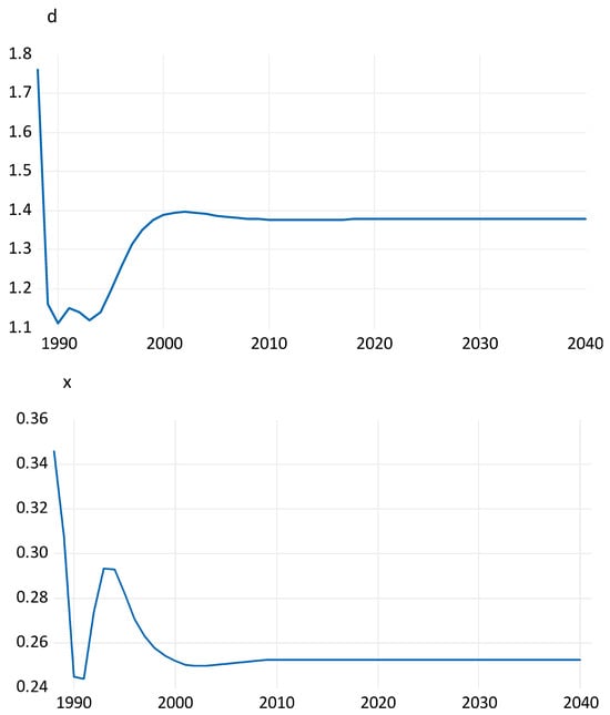
Figure 2. Forecast for a VAR in foreign debt, d = D/K_f, and exports, x = pX/K_f, (both in percent of stock of foreign capital goods) with horizontal lines out of sample for 2021–2040.

The results from this VAR analysis would suggest that the steady states on the most far right of Figure 1 are more plausible for Brazil than the other two.

4. Discussion

This section discusses literature that can be related to the model. Properties of comparable models with or without limited exports are as follows.

The empirical literature explains foreign debt through current account. The theoretical literature explains foreign debt via investment–savings difference. The model of this paper combines the two because imported capital goods appear in both, the current account and the investment savings difference.

The income elasticity argument of Engel (1857), Prebisch (1959), and Marquez (1985a) for developing countries, as well as Marquez (1985b) and others for the USA, holds in a growth model with domestic and imported capital goods explaining foreign deficits and debt besides growth itself.

The terms of trade can increase, fall, or remain constant in the steady state and in the transition as in the modern literature on structural change. The model of Acemoglu and Ventura (2002) has only terms of trade falling through relatively strong capital growth, but not the role of export demand.16

There is possibly permanent structural change in the use of domestic and foreign capital goods, implying a relative shrinkage or expansion of the investment goods sector depending on the development of the terms of trade. Price effects thereby are of long-term nature and do not phase out in steady states, unless the foreign and domestic driving forces of growth are exactly equally strong.

The model is related to several branches of empirical literature, which can perhaps be better understood with the help of the growth model with domestic and imported capital goods paid for by exports and foreign debt. Developing and developed countries’ growth is dependent on world income growth in the export function, not only technical change. There is a relation of exports and growth for OECD and EU countries. Thorbecke (2015) argues that for Japan exports depend on importing countries’ income. Kónya (2006) shows the (two-way) causal impact of several OECD countries’ exports on growth. Maneschiöld (2008) finds cointegration between exports and GDP for Argentina, Brazil, and Mexico; Tang et al. (2011) find it for Hong Kong, Korea, Singapore, and Taiwan; Gupta (2011) for India; and Adelakun et al. (2025) for 22 African countries.

Esfahani (1991) for semi-industrialized countries; Riezman et al. (1995) for 30 of 126 countries (emphasizing the link from imports to production capacity); Thangavelu and Rajaguru (2004) and Hye et al. (2013) and Ahmad et al. (2018) for five Asian countries; Awokuse (2008) for Argentina, Colombia, and Peru; and Ibarra (2011) for Mexico suggest that the export–growth link is intermediated by imports as it is in our model.

Lee (1995) provides cross-section evidence that shifts the argument most clearly to imported capital goods. Cavallo and Landry (2010) find that 20 to 30 percent of US growth stems from imported capital goods. Herrerias and Orts (2013) emphasize the role of imported capital goods for China, Abo-Zaid (2010) for Israel, and Arawomo (2014) for countries of the West Africa Monetary Zone that comprises Nigeria, Ghana, Gambia, Guinea, Liberia, and Sierra Leone, and Co (2023) emphasizes the same for sub-Saharan Africa. Caselli (2018) provides evidence for Mexican manufacturing plants, and Mo et al. (2021) for Chinese manufacturing firms, both suggesting that imported capital goods are more important then imported intermediates. Bakari (2022) shows that exports strengthen the impact of investment on growth in 28 developed countries. Growth rates in these papers and our model depend on the same forces as structural change: income elasticities, rates of technical change, and endowment growth.

All these results together suggest that the nexus from imported capital goods and exports to growth does not only hold for developing countries but also for developed countries. The reason is that the small country assumption of an infinite price elasticity does not hold. Houthakker and Magee (1969) find price elasticities between −0.3 for Italy and −2.4 for South Africa and for twelve OECD countries. Moreover, income elasticities are below unity for USA, UK, and South Africa but above 1.18 and 3.5 for the other countries. Romero and McCombie (2018) find values in this range for sectors of seven EU countries. Price elasticities from Stern et al. (1976) and Faini et al. (1992) mentioned above are in the range of −1 and −2.1. Aiello et al. (2014) find price inelastic exports except for France (−2) and mostly large income elasticities for the other countries. Kumar (2011) finds that long-run income elasticities range between 1 and 1.3, and the relative price elasticities range between −1 and −1.4 for India, China, The Philippines, Indonesia, Singapore, and Malaysia. Ketenci (2014) finds large income elasticities of export demand and mostly short- and long-run price elasticities near zero for BRICS countries, Indonesia, and Turkey. Compared to high price elasticities this means that strong demand may turn into higher prices, but this does not weaken the export demand. Indian sectors have income elasticities near 1.5 and price elasticities between −086 and 1.14 (Raissi & Tulin, 2015). Cao and Kozicki (2017) show for Canada that ‘In most years of the 2000s, the contribution of the terms of trade became significant in real income growth, whereas that of total factor productivity growth was stagnant’. Basnet et al. (2021) state that the positive relation between terms of trade and growth is a standard result in the literature. In our model this latter result implies that export demand growth dominates growth through technical change.

In many papers the link between exports and growth is not confirmed.17 This may be because imports are not included (besides nonlinearity, asymmetry, and other econometric issues; see Lim and Ho (2013); Ben-Salha et al. (2023). If imports are included but the link is still not found, this may be because imports also include imported consumption goods, which are of course not good for growth. Moreover, the link seems to be weaker for imported intermediate goods than for imported capital goods. Consequently, papers analyzing the link between R&D, productivity, and exports (Máñez et al., 2015) and similar related questions should include imported capital goods in future research to get the attribution straight if the data situation allows doing so. The value of having a clear explicit growth model as in this paper is exactly in seeing the requirements for empirical work more clearly than when only specifying regressions with omitted variables, which in VECM models have the additional implication of one or more missing equations and risk of an omitted variable in each equation.

A non-convergence of the trade balance or the current account to zero is not a valid argument against BPCG (McCombie, 2011), or against neoclassical versions as Ziesemer (1995b), or this paper, even when foreign debt growth is constrained, because differences between investment domestic savings or imports and exports are quite normal in international economic thinking, and our model has three steady states in which a constant debt ratio implies that debt is growing with the same rate as the denominator. BPCG models differ from our model in that they do not lean on imported capital goods and the imperfect substitutability with domestic and foreign capital goods. Moreover, they have exogenous and constant terms of trade; therefore, price adjustments cannot lead to substitutions mitigating growth and debt problems. In our model this is possible but may have limited effects depending on price and income elasticities of export demand and substitution between domestic and foreign capital goods. Exports and debt, both per unit of foreign capital, are constant in the long run in this paper, but growth is constrained by limited exports. By implication, in the steady state, exports and debt have growth with the same sign, which is that of the foreign capital stock. Outside the steady state, the arrows in Figure 1 show that any sign for the relation between exports and debt growth is possible. For example, Odhiambo (2022) finds positive (not all significant) Granger causality relations between growth of exports and foreign debt for low- and middle-income countries in sub-Saharan Africa.

5. Summary and Conclusions

Essentially, the Solow–Swan assumption of one good used in the utility and the production function is doubled: two countries each have one good and both goods are used in both utility and production functions.

Trade and permanent growth are linked in this model because statically imperfectly substitutable domestic and foreign capital goods with elasticity of substitution unity are dynamic complements along the growth path. Permanent imports of foreign capital goods with payments through exports or foreign debt give a permanent role to trade. Therefore, income and finite price elasticities of export demand appear in the long run growth formulas

Only in two special cases do we get the standard neoclassical results of the Solow–Swan model: if the effects of world income growth and technical change are equally strong or in the case of infinite price elasticities of export demand.

Trade enhances growth because it brings into the model foreign capital goods, which would have to be invented by every country on its own in the absence of trade. Stronger export growth improves the terms of trade. Higher domestic to foreign prices lead to leaning more on imported machinery and to more capital accumulation.

When exports are limited under endogenous terms of trade, debt is used first to pay for imported capital goods. The value of foreign debt is about as high as the value of accumulated imported capital goods for our five calibration cases. For a VAR with data from Brazil, it is even higher.

Imported capital goods appear in the formula for investment and in the formula for imports. Finding the value of accumulated debt from either only the investment–savings difference or only the current account deficit is not possible in this model. The real policy of limiting foreign debt must reduce both the investment–savings difference and the import–export difference.

The structure of the model provides a perspective for the interpretation of several strands of the literature: the export–growth nexus, its extension to include imports, its variants to emphasize imported intermediates and, more importantly, imported capital goods, and the literature linking all these variables to the terms of trade as a flexible relative price that commands the ratio of domestic and foreign capital goods. The model indicates that it is more meaningful to see these strands of literature as complementary rather than competing.

We will leave the endogenization of high interest rates via spreads by international consortia for future research. In the presence of bail-out practices, it is unclear how important it is.

References

- Abo-Zaid, S. M. (2010). The trade-growth relationship in Israel revisited: Evidence from annual data, 1960–2004. Review of Middle East Economics and Finance, 6(3), 4. [Google Scholar] [CrossRef]
- Acemoglu, D., & Ventura, J. (2002). The world income distribution. The Quarterly Journal of Economics, 117(2), 659–694. [Google Scholar] [PubMed]
- Adelakun, O. J., Ojo, O. O., & Mpungose, S. (2025). Empirical re-investigation into the export-led growth hypothesis (ELGH): Evidence from EAC and SADC economies. Economies, 13(6), 175. [Google Scholar] [CrossRef]
- Ahmad, F., Draz, M. U., & Yang, S. C. (2018). Causality nexus of exports, FDI and economic growth of the ASEAN5 economies: Evidence from panel data analysis. The Journal of International Trade & Economic Development, 27(6), 685–700. [Google Scholar] [CrossRef]
- Aiello, F., Bonanno, G., & Via, A. (2014). Do export price elasticities support tensions in currency markets? Evidence from China and six OECD countries (MPRA Paper No. 56727). Munich Personal RePEc Archive. [Google Scholar]
- Amano, A. (1965). International capital movements and economic growth. Kyklos, 18(4), 693–699. [Google Scholar] [CrossRef]
- Arawomo, D. F. (2014). Nexus of capital goods import and economic growth: Evidence from panel ARDL model for WAMZ. Journal of International and Global Economic Studies, 7(2), 32–44. [Google Scholar]
- Awokuse, T. O. (2008). Trade openness and economic growth: Is growth export-led or import-led? Applied Economics, 40(2), 161–173. [Google Scholar] [CrossRef]
- Bakari, S. (2022). The nexus between domestic investment and economic growth in developed countries: Do exports matter? (MPRA Paper No. 114418). Munich Personal RePEc Archive. [Google Scholar]
- Bardhan, P., & Lewis, S. (1970). Models of growth with imported inputs. Economica, 37(148), 373–385. [Google Scholar] [CrossRef]
- Basnet, H. C., Devkota, S. C., & Upadhyay, M. P. (2021). Terms of trade and real domestic income: New evidence from South and Southeast Asia. International Journal of Finance & Economics, 26(3), 4315–4331. [Google Scholar]
- Ben-Salha, O., Abid, A., & El Montasser, G. (2023). Linear and nonlinear causal linkages between exports and growth in next eleven economies. Journal of the Knowledge Economy, 14(2), 1194–1226. [Google Scholar] [CrossRef]
- Boppart, T. (2014). Structural change and the Kaldor facts in a growth model with relative price effects and non-Gorman preferences. Econometrica, 82(6), 2167–2196. [Google Scholar] [CrossRef]
- Buffie, E. F. (1992). On the condition for export-led growth. The Canadian Journal of Economics/Revue Canadienne d’Economique, 25(1), 211–225. [Google Scholar] [CrossRef]
- Burenstam-Linder, S. (1961). An essay on trade and transformation [Doctoral dissertation, Stockholm School of Economics]. [Google Scholar]
- Cao, S., & Kozicki, S. (2017). Real GDI, productivity, and the terms of trade in Canada. Review of Income and Wealth, 63(S1), S134–S148. [Google Scholar] [CrossRef]
- Caselli, M. (2018). Do all imports matter for productivity? Intermediate inputs vs. capital goods. Economia Politica, 35(2), 285–311. [Google Scholar] [CrossRef]
- Cavallo, M., & Landry, A. (2010). The quantitative role of capital goods imports in us growth. American Economic Review, 100(2), 78–82. [Google Scholar] [CrossRef]
- Co, C. Y. (2023). Export capacity and capital stock augmentation through imports: Evidence from Sub-Saharan African countries. South African Journal of Economics, 91(3), 273–305. [Google Scholar] [CrossRef]
- Engel, E. (1857). Die Productions- und Consumptionsverhaeltnisse des Koenigsreichs Sachsen. Zeitschrift des Statistischen Bureaus des Koniglich Sachsischen Ministeriums des Inneren, 8, 1–54. (In German) [Google Scholar]
- Esfahani, H. S. (1991). Exports, imports, and economic growth in semi-industrialized countries. Journal of Development Economics, 35(1), 93–116. [Google Scholar] [CrossRef]
- Faini, R., Clavijo, F., & Senhadji-Semlali, A. (1992). The fallacy of composition argument: Is it relevant for LDCs’ manufactures exports? European Economic Review, 36(4), 865–882. [Google Scholar] [CrossRef]
- Fosu, A. K., Getachew, Y. Y., & Ziesemer, T. H. W. (2016). Optimal public investment, growth, and consumption: Evidence from African countries. Macroeconomic Dynamics, 20(8), 1957–1986. [Google Scholar] [CrossRef]
- Grossman, G. M., & Helpman, E. (1991). Innovation and growth in the global economy. MIT Press. [Google Scholar]
- Gupta, R. (2011). What causes trade-led growth in India? Margin: The Journal of Applied Economic Research, 5(3), 293–310. [Google Scholar] [CrossRef]
- Habiyaremye, A., & Ziesemer, T. H. W. (2012). Export demand elasticities and productivity as determinants of growth: Estimates for Mauritius. Applied Economics, 44(9), 1143–1158. [Google Scholar] [CrossRef]
- Hamada, K. (1966). Economic growth and long-run capital movements. Yale Economic Essays, 6, 49–96. [Google Scholar]
- Harris, D. J. (1975). The theory of economic growth: A critique and reformulation. The American Economic Review, 65(2), 329–337. [Google Scholar]
- Herrerias, M. J., & Orts, V. (2013). Capital goods imports and long-run growth: Is the Chinese experience relevant to developing countries? Journal of Policy Modeling, 35(5), 781–797. [Google Scholar] [CrossRef]
- Houthakker, H. S., & Magee, S. P. (1969). Source income and price elasticities in world trade. The Review of Economics and Statistics, 51(2), 111–125. [Google Scholar] [CrossRef]
- Hye, Q. M. A., Wizarat, S., & Lau, W. Y. (2013). Trade-led growth hypothesis: An empirical analysis of South Asian countries. Economic Modelling, 35, 654–660. [Google Scholar] [CrossRef]
- Ibarra, C. A. (2011). Import elasticities and the external constraint in Mexico. Economic Systems, 35(3), 363–377. [Google Scholar] [CrossRef]
- Johnson, H. G. (1953). Equilibrium growth in an international economy. Canadian Journal of Economics, 19(4), 478–500. [Google Scholar]
- Ketenci, N. (2014). Trade elasticities, commodity prices, and the global financial crisis: Evidence from BRIICS countries and Turkey. Global Journal of Emerging Market Economies, 6(3), 233–256. [Google Scholar] [CrossRef]
- Kónya, L. (2006). Exports and growth: Granger causality analysis on OECD countries with a panel data approach. Economic Modelling, 23(6), 978–992. [Google Scholar] [CrossRef]
- Kravis, I. B. (1970). Trade as a handmaiden of growth: Similarities between the nineteenth and twentieth centuries. The Economic Journal, 80(320), 850–872. [Google Scholar] [CrossRef]
- Kumar, S. (2011). Estimating export demand equations in selected Asian countries. Journal of Chinese Economic and Foreign Trade Studies, 4(1), 5–16. [Google Scholar] [CrossRef]
- Lee, J. W. (1995). Capital goods imports and long-run growth. Journal of Development Economics, 48(1), 91–110. [Google Scholar] [CrossRef]
- Leung, H. M. (2000). Trade and growth: A theoretical exploration into foreign debts by NICs. Economic Modelling, 17(1), 35–47. [Google Scholar] [CrossRef]
- Lim, S. Y., & Ho, C. M. (2013). Nonlinearity in ASEAN-5 export-led growth model: Empirical evidence from nonparametric approach. Economic Modelling, 32, 136–145. [Google Scholar] [CrossRef]
- Maneschiöld, P. O. (2008). A note on the export-led growth hypothesis: A time series approach. Cuadernos de Economía, 45(132), 293–302. [Google Scholar]
- Mankiw, N. G., Romer, D., & Weil, D. N. (1992). A contribution to the empirics of economic growth. Quarterly Journal of Economics, 107(2), 407–437. [Google Scholar]
- Marquez, J. (1985a). Foreign exchange constraints and growth possibilities in the LDCs. Journal of Development Economics, 19(1–2), 39–57. [Google Scholar]
- Marquez, J. (1985b, July). Currency substitution and the new divisia monetary aggregates: The US case (International Finance Discussion papers 275). Princeton University. [Google Scholar]
- Máñez, J. A., Rochina-Barrachina, M. E., & Sanchis-Llopis, J. A. (2015). The dynamic linkages among exports, R & D and productivity. The World Economy, 38(4), 583–612. [Google Scholar]
- McCombie, J. S. L. (2011). Criticisms and defences of the balance-of-payments constrained growth model: Some old, some new. PSL Quarterly Review, 64(259), 353–392. [Google Scholar]
- McKinnon, R. I. (1964). Foreign exchange constraints in economic development and efficient aid allocation. The Economic Journal, 74(294), 388–409. [Google Scholar] [CrossRef]
- Mo, J., Qiu, L. D., Zhang, H., & Dong, X. (2021). What you import matters for productivity growth: Experience from Chinese manufacturing firms. Journal of Development Economics, 152, 102677. [Google Scholar] [CrossRef]
- Mutz, C., & Ziesemer, T. (2008). Simultaneous estimation of income and price elasticities of export demand, scale economies and total factor productivity growth for Brazil. Applied Economics, 40(22), 2921–2937. [Google Scholar] [CrossRef]
- Nunes-Pereira, F., & Moura, M. G. (2024). On the survival of a flawed theory of capital: Mainstream economics and the Cambridge capital controversies. Cambridge Journal of Economics, 48(2), 169–186. [Google Scholar] [CrossRef]
- Nurkse, R. (1961). Equilibrium and growth in the world economy (G. Haberler, & R. M. Stern, Eds.). Harvard University Press. (Original work published 1944). [Google Scholar]
- Odhiambo, N. M. (2022). Is export-led growth hypothesis still valid for sub-Saharan African countries? New evidence from panel data analysis. European Journal of Management and Business Economics, 31(1), 77–93. [Google Scholar] [CrossRef]
- Onitsuka, Y. (1974). International capital movements and the patterns of economic growth. The American Economic Review, 64(1), 24–36. [Google Scholar]
- Perkins, D. H., Radelet, S., Lindauer, D. L., & Block, S. A. (2013). Economics of development (7th ed.). Norton. [Google Scholar]
- Pesaran, M. H. (2015). Time series and panel data econometrics. Oxford University Press. [Google Scholar]
- Prebisch, R. (1950). The economic development of Latin America and its principal problems. Economic Bulletin for Latin America, 7, 1–22. [Google Scholar]
- Prebisch, R. (1959). Commercial policy in the underdeveloped countries. American Economic Review, 49, 251–273. [Google Scholar]
- Raissi, M., & Tulin, V. (2015). Price and income elasticity of Indian exports—The role of supply-side bottlenecks (IMF Working Paper 15/161). International Monetary Fund. [Google Scholar]
- Riezman, R. G., Summers, P. M., & Whiteman, C. H. (1995). The engine of growth or its handmaiden? A time-series assessment of export-led growth (University of Iowa Department of Economics Working Paper Series, 95-16). University of Iowa. [Google Scholar]
- Rivera-Batiz, L. A., & Romer, P. M. (1991). Economic integration and endogenous growth. The Quarterly Journal of Economics, 106(2), 531–555. [Google Scholar] [CrossRef]
- Rivera-Batiz, L. A., & Xie, D. (1993). Integration among unequals. Regional Science and Urban Economics, 23(3), 337–354. [Google Scholar] [CrossRef]
- Romero, J. P., & McCombie, J. S. (2018). Thirlwall’s law and the specification of export and import functions. Metroeconomica, 69(2), 366–395. [Google Scholar] [CrossRef]
- Singer, H. W. (1999). Beyond terms of trade—Convergence and divergence. Journal of International Development, 11, 911–916. [Google Scholar] [CrossRef]
- Stern, R. M., Francis, J., & Schumacher, B. (1976). Price elasticities in international trade. Macmillan. [Google Scholar]
- Tang, C. F., Lai, Y. W., & Ozturk, I. (2011). The stability of export-led growth hypothesis: Evidence from Asia’s four little dragons (MPRA Paper No. 27962). Munich Personal RePEc Archive. [Google Scholar]
- Thangavelu, S. M., & Rajaguru, G. (2004). Is there an export or import-led productivity growth in rapidly developing Asian countries? a multivariate VAR analysis. Applied Economics, 36(10), 1083–1093. [Google Scholar] [CrossRef]
- Thorbecke, W. (2015). Understanding Japan’s capital goods exports. The Japanese Economic Review, 66(4), 536–549. [Google Scholar] [CrossRef]
- Ziesemer, T. H. W. (1995a). Economic development and endogenous terms of trade determination: Reexamination and reinterpretation of the Prebisch-Singer thesis. UNCTAD Review, 17–34, (Reprinted in 1998, Export-led versus balanced growth in the 1990s (Singer, S. H., Hatti, N., & Tandon, R., Eds.). [NEW WORLD ORDER SERIES VOL. XIII]. B.R. Publishing Corporation Ltd.). [Google Scholar]
- Ziesemer, T. H. W. (1995b). Growth with imported capital goods, limited export demand and foreign debt. Journal of Macroeconomics, 17(1), 31–53. [Google Scholar] [CrossRef]
- Ziesemer, T. H. W. (1998). A Prebisch-Singer growth model and the debt crises. In Development economics and policy: The conference volume to celebrate the 85th birthday of professor sir Hans Singer (pp. 300–317). Palgrave Macmillan. [Google Scholar]
- Ziesemer, T. H. W. (2005). Growth with perfect capital movements in CES: US Debt Dynamics and model estimation (MERIT RM 2005-014). Maastricht Economic Research Institute on Innovation and Technology (MERIT). [Google Scholar]
- Ziesemer, T. H. W. (2014). Country terms of trade: Trends, unit roots, over-differencing, endogeneity, time dummies, and heterogeneity. International Review of Applied Economics, 28(6), 767–796. [Google Scholar] [CrossRef]
- Ziesemer, T. H. W. (2023a). Labour-augmenting technical change data for alternative elasticities of substitution: Growth, slowdown, and distribution dynamics. Economics of Innovation and New Technology, 32(4), 449–475. [Google Scholar] [CrossRef]
- Ziesemer, T. H. W. (2023b). Semi-endogenous growth in a non-Walrasian DSEM for Brazil: Estimation and simulation of changes in foreign income, human capital, R&D, and terms of trade. Economic Change and Restructuring 56, 1147–1183. [Google Scholar]
- Ziesemer, T. H. W. (2024). Estimation of a production function of Brazil with domestic and foreign capital stock, 1991–2017. Applied Econometrics and International Development, 24(2), 103–128. [Google Scholar]
Disclaimer/Publisher’s Note: The statements, opinions and data contained in all publications are solely those of the individual author(s) and contributor(s) and not of MDPI and/or the editor(s). MDPI and/or the editor(s) disclaim responsibility for any injury to people or property resulting from any ideas, methods, instructions or products referred to in the content. |
© 2026 by the author. Licensee MDPI, Basel, Switzerland. This article is an open access article distributed under the terms and conditions of the Creative Commons Attribution (CC BY) license.