Trajectories, Fairness, and Convergence: Global Development in a Multidimensional Econo-Environmental Capability Space

Abstract

This study examines global econo-environmental capability for 118 countries over 1995 to 2024 using a five-lens framework covering productive capacity (PC), developmental momentum (DM), resource efficiency (RE), degradation and depletion ratio (DDR), and remaining development potential (RDP). Using pooled k-means, a stable four archetype typology is identified and shown to persist over time. The analysis assesses how archetypes characterize country–year outcomes (RQ1), whether cross-sectional fairness is changing and relates to frontier slowdown (RQ2), and how archetypes, distance, and regional context shape transition probabilities and club convergence (RQ3). Inequality in five-dimensional capability declines slightly over the period (Gini from 0.109 to 0.092 and Palma from 1.563 to 1.464), implying modest convergence rather than increasing polarization. Average capability also improves, with larger gains for initially distant countries and smaller gains near the frontier, which is consistent with mild club convergence. Regionally, high capability cases are concentrated in Western Europe and North America, while sustained upgrading is observed in parts of Eastern Europe, mixed stability is observed in East and Central Asia, and selective advances are observed in ASEAN. Policy implications should be based on a country’s archetype and its distance to the capability ideal. Lagging countries should prioritize diffusion of proven high efficiency options and basic capability building, while frontier countries should priorities innovation, structural change, and deeper decarbonization. Policy emphasis should be updated as countries move within the capability space over time.

1. Introduction

The challenge of harmonizing economic growth with environmental sustainability remains a central issue in contemporary global development discourse. Since the publication of the Brundtland Report (WCED, 1987), policymakers and researchers have been exploring pathways to reconcile the pursuit of material prosperity with the imperative of preserving ecological systems. This challenge is further complicated by the structural realities of resource scarcity and the contested evolution of sustainability discourses (Redclift, 2005; Sneddon et al., 2006). This debate is evident in the Environmental Kuznets Curve literature. Early optimism that income growth would automatically reduce environmental pressures has been undermined by mixed empirical evidence (Stern et al., 1996). Ecological footprint evidence for OECD countries has also questioned the validity of a single inverted U pathway (Chu & Hoang, 2022). This unresolved tension highlights the need for analytical frameworks and empirical tools that assess sustainability outcomes while also capturing heterogeneous and dynamic processes through which countries navigate trade-offs between development and environmental preservation.

An evolutionary perspective implies that environmental performance can follow multiple pathways, which makes static assessment insufficient. The pivotal inquiry concerns how environmental performance evolves as a dynamic state shaped by long-run interactions among growth, efficiency, and resource use, and how these patterns can be recovered empirically from trajectory aware evidence (Agusdinata et al., 2020). Countries that appear similar at a given point in time may have reached that position through different trajectories, including efficiency upgrading, depletion driven adjustment, or structural momentum (Terluin, 2003). Similar outcomes can also be produced through differing combinations of domestic capacity and external forces. These evolutionary dynamics are difficult to recover from static assessments. Sustainability transitions research has also shifted over time (Stefani et al., 2022). Methodologies that trace transitions, stability, and long-run movement across multidimensional state spaces are therefore required to understand pathways and to derive lessons for more efficient and fair sustainable transitions (Agusdinata et al., 2020; Alotaiq, 2024; Renou-Maissant et al., 2022).

One of the primary challenges is the multidimensional nature of environmental performance. This complexity reflects broader conceptual debates regarding the definition and operationalization of sustainability (Osorio et al., 2005; Ruggerio, 2021). Traditional reliance on singular indicators, such as per capita carbon emissions, energy intensity, or deforestation rates, provides clarity and comparability. However, reality can be oversimplified when environmental performance is reduced to isolated metrics. Such metrics seldom capture systemic interactions among economic activity, resource efficiency, and ecological limits, nor do they adequately reflect how structural shifts and innovation dynamics mediate these interactions (Renou-Maissant et al., 2022). In this context, multidimensional frameworks that jointly track several capability dimensions can enhance understanding of development pathways by revealing patterns, trade-offs, and synergies that single measures may overlook (Agusdinata et al., 2020; Alotaiq, 2024; Moallemi et al., 2022; Eisenack et al., 2019).

In response to the need for more comprehensive perspectives, composite indices have been developed. Key frameworks include the Environmental Sustainability Index (Esty et al., 2005), its successor the Environmental Performance Index (Hsu et al., 2016), the Ecological Footprint (Wackernagel & Rees, 1996), and the Planetary Boundaries approach (Rockström et al., 2009; Steffen et al., 2015). These indices benchmark national performance across multiple dimensions. However, when multidimensional information is condensed into single scores or rankings, cross-sectional comparability is prioritized over dynamic interpretation, and countries’ movement within multidimensional state spaces is obscured (Haque, 2000). Comparative evidence further shows that different national sustainability indices can yield conflicting assessments for the same countries (Siche et al., 2008). While pillar framing supports coverage and accountability, a capability perspective concentrates on a country’s capacity to act, learn, coordinate, and sustain improvement, and facilitates assessment relative to an explicit ideal, including distance-conditioned dynamics, permanence, and reversals. Nevertheless, capability-oriented evolutionary evidence remains limited in cross-country sustainability assessment.

Multidimensional sustainability assessment is commonly pursued through composite indices and pillar-based frameworks that summarize performance across domains (Bluszcz, 2016; Siche et al., 2008; Alotaiq, 2024). This pillar-based tradition has been valuable for descriptive benchmarking. An alternative perspective is offered by the capability approach, which evaluates systems through achieved functioning and the real opportunities that enable them, rather than through input volumes alone (Sen, 1999). When applied to sustainability, attention is directed to capacities that support sustained improvement under constraint. This shift helps identify which capabilities are holding progress back and which ones reinforce each other, rather than only describing domain coverage. Nevertheless, capability-oriented evaluation remains limited in multidimensional cross-country research on sustainability progression.

This study addresses three gaps in the literature. First, environmental sustainability progression is commonly assessed using pillar-based composites, while explicitly capability-oriented evaluations remain limited. Second, multi-indicator assessments have rarely been extended to track capability evolution over time within a consistent multidimensional state space. Third, limited evidence has been developed on how starting conditions, regional context, and structural constraints shape countries’ sustainability pathways, including their movement between archetypes, within environmental capability space. Data for 1995–2024 are used, representing the longest period for which a consistent five-lens environmental capability dataset is available with broad country coverage. This coverage supports examination of long-run trajectories and dynamics. Based on these gaps, three research questions are examined:

• RQ1: How can countries be characterized by a set of stable archetypes in the five-lens environmental capability framework over 1995–2024, and how do these archetypes behave and exhibit persistence over time?
• RQ2: Is cross-sectional inequality in capability small and declining, and how is fairness related to a deceleration near the frontier as the distance to the ideal state becomes smaller?
• RQ3: How do starting distance, archetype membership, and regional context shape transition probabilities, permanence, and reversals, and do these mechanisms produce tempered club convergence?

This study advances the literature by operationalizing environmental sustainability progression as evolutionary movement within a five-lens capability space and by recovering stable archetypes that can be compared consistently over time. Each country–year is represented as a position in a multidimensional environmental capability space, which enables trajectories, persistence, and reversals to be examined directly. In addition, distributional patterns, mobility between archetypes, regional structure, and performance improvement within the capability space are examined, with distance to the ideal reference point serving as an analytical benchmark and the permanence rule supporting interpretation of sustained archetype membership and transition stability. These design elements complement convergence perspectives by clarifying how countries move between capability profiles over time. In this way, dynamic capability evolution is emphasized over static benchmarking, and evidence is provided to inform more equitable transition strategies from an environmental capability perspective.

2. Literature Review

Environmental performance has frequently been evaluated using composite indices and benchmarking exercises that summarize national pressures and responses. However, outputs are commonly reported as cross-sectional ranks or single year scores, which limits inference on temporal progression (Esty et al., 2005; Hsu et al., 2016). Earth system perspectives have further contextualized national outcomes within biophysical thresholds and planetary limits, yet national benchmarking typically remains static even when dynamic risks and tipping points are implied (Wackernagel & Rees, 1996; Rockström et al., 2009; Steffen et al., 2015).

Composite indices can yield divergent country rankings because results are sensitive to indicator selection and normalization choices. This variability supports preserving dimensional structure rather than relying on singular ranks (Siche et al., 2008; Bluszcz, 2016). Income based narratives such as the Environmental Kuznets Curve are pollutant specific and contingent on structural conditions. Improvement therefore cannot be inferred from income alone and requires assessment against explicit targets (Stern et al., 1996; OECD, 2002). A distance to ideal framing can provide a consistent basis for evaluating attainment and dispersion across multiple dimensions. In this framing, fairness can be interpreted through cross-sectional dispersion measures, while temporal change can be examined through distance conditioned improvement. Research on limits and scarcity further supports a frontier aware interpretation, since diminishing returns and stock effects imply that progress may slow near biophysical or institutional constraints (Ekins, 1993; Halvorsen & Smith, 1984; Krautkraemer, 1998).

Temporal change is shaped by structure, displacement, and scarcity, so progress cannot be inferred from single drivers. Shifts in composition and technology can reduce pressure, yet gains vary across country structures, so similar changes can yield different environmental outcomes (Gilli et al., 2013; Amann et al., 2013; Renou-Maissant et al., 2022). Trade can relocate emissions and resource use. Local improvement can therefore be observed in importing economies while embodied pressures rise elsewhere, which motivates cross border accounting (Peters et al., 2011; Jackson, 2009; Basu et al., 2022). Near physical or institutional constraints, costs and shadow prices can rise and adjustment can become nonlinear, so improvement may slow despite continued effort (Halvorsen & Smith, 1984; Krautkraemer, 1998; Stern et al., 1996). These mechanisms suggest that initial distance from an explicit ideal can condition subsequent change, motivating distance conditioned metrics that can evaluate whether progress decelerates as the frontier is approached.

Clustering techniques condense multidimensional sustainability data into interpretable country typologies. However, most studies focus on snapshots and have limited ability to document persistence or transitions over time. Recent applications have identified archetypes based on social, environmental, and production indicators, yet trajectories and centroid stability are rarely traced, which constrains evolutionary inference (Küppers et al., 2019; Partelow et al., 2025; Alotaiq, 2024). Methodological syntheses recommend treating archetypes as transferable constructs with defined validity domains. Feedbacks and trade-offs can generate rebounds and instability, so stability validation is required before policy interpretation (Sietz et al., 2019; Eisenack et al., 2019; Moallemi et al., 2022). Related research on distribution dynamics and club convergence has further indicated multiple steady state groups and heterogeneous adjustment speeds shaped by initial conditions and regional structures (Panopoulou & Pantelidis, 2009; Eleftheriou et al., 2024; Erdogan & Okumus, 2021).

Taken together, the literature indicates three recurrent limitations that align with the research questions. First, archetype and typology studies have often been treated cross-sectionally, while multi decade trajectories and persistence patterns remain under examined, which limits evolutionary inference (Küppers et al., 2019; Partelow et al., 2025; Alotaiq, 2024). Second, fairness in capability attainment against defined ideals has rarely been quantified using distributional measures such as Gini and Palma, and frontier behavior has often been discussed descriptively rather than tested using distance conditioned improvement (Bluszcz, 2016; OECD, 2002). Third, mobility mechanisms across capability states remain under examined, since transition probabilities, durability, and reversals are rarely estimated and related to initial distance and regional context, despite evidence of multiple steady states and heterogeneous adjustment speeds in club convergence research (Panopoulou & Pantelidis, 2009; Eleftheriou et al., 2024; Renou-Maissant et al., 2022). Table 1 summarizes representative studies on country environmental archetypes and related trajectory evidence, highlighting methods, scope, and relevance to the research questions.

Table 1. Literature review on country environmental archetypes trajectories and evolution.

Reference	Method	Scope	Timeframe	Focus	Relevance
Agusdinata et al. (2020)	CART classification (country archetypes)	Global	1980 to 2014	CO2 per capita trajectory (slope); GDP growth trend	Supports multi-path emissions archetypes beyond EKC; intensity focus (RQ1, RQ3)
Alotaiq (2024)	k-means clustering	Global	2015 to 2020	Renewables share; electrification; GDP growth; HDI; governance (WGI);	Motivates archetype-specific transition routes; not region-generic (RQ3)
Moallemi et al. (2022)	Systems archetype analysis (causal-loop)	Global	—	SDG interaction patterns; feedbacks; policy levers	Alerts to trade-offs and rebound; monitor reversals (RQ3)
Eisenack et al. (2019)	Archetype analysis framework (conceptual)	Global	—	Conceptual framework	Advocates transferable, scale-aware archetypes with validity domains (RQ1)
Küppers et al. (2019)	k-means clustering	Global (140 countries)	2015 to 2015	49 socioeconomic, climatic, and energy indicators	Suggests tentative clubs; requires dynamic tracking for persistence (RQ3)
Partelow et al. (2025)	Hierarchical clustering	Global (150 countries)	2015 to 2019	42 indicators across social, economic, governance, environmental, and production	Notes risk constraints on mobility and reversal risk (RQ3)
Pedde et al. (2019)	Scenario archetypes (SSP/worldviews)	Global and subnational	—	SSP narratives; STEEP indicators; worldview coding	Emphasizes context dependence; global families fragment locally (RQ3)
Sietz et al. (2019)	Methodological synthesis of archetype analysis	Global	—	Sustainability systems	Prioritizes temporal stability validation over static snapshots (RQ1)
Hansen et al. (2018)	Special issue introduction	Global (developing-country focus)	—	Country sustainability transitions	Highlights durability factors; nurture niches and value-chain links (RQ3)
Eleftheriou et al. (2024)	Phillips–Sul club convergence	Global (137 countries)	1990 to 2019	SDI inputs: CO2 per capita; material footprint; HDI components	Shows club-specific convergence; paths differ by development stage (RQ3)
Erdogan and Okumus (2021)	Phillips–Sul club convergence	Global (89 countries)	1961 to 2016	Ecological footprint per capita	Documents multiple steady states; aggregate convergence misleads (RQ3)
Arogundade et al. (2023)	Phillips–Sul club convergence	Global (189 countries)	1990 to 2017	Ecological footprint per capita	Regional clubs shaped by starting pressure and resources (RQ3)
Haider and Akram (2019)	Phillips–Sul club convergence	Global (77 countries)	1961 to 2014	Ecological footprint per capita; carbon footprint per capita	Two steady states; design policy by club (RQ3)
Emir et al. (2019)	Phillips–Sul club convergence	EU (country level)	1990 to 2016	CO2 intensity (kg CO2 per kg oil-equivalent energy)	EU shows multiple clubs; differentiate targets (RQ3)
Panopoulou and Pantelidis (2009)	Phillips–Sul club convergence with club identification	Global 128 countries)	1960 to 2003	CO2 emissions per capita	Early convergence splits into two clubs; track permanence and reversals (RQ3)
Gómez and Rodríguez (2024)	Phillips–Sul club convergence	Americas (7 countries)	1990 to 2022	Energy consumption per capita; CO2 per capita; Ecological footprint per capita; energy intensity; load capacity factor	Indicator-specific clubs; region- and indicator-tailored pathways (RQ3)
Ulucak and Apergis (2018)	Phillips–Sul club convergence	EU (country level; 20)	1961 to 2013	Ecological footprint per capita	EU convergence rejected; persistent multiple clubs require differentiation (RQ3)
Ma et al. (2025)	Product-space network analysis (“SDG space”)	Global (country level; 166)	2000 to 2022	96 SDG indicators	Polarized specialization; use distance-aware targeting and monitor reversals (RQ3)
Amann et al. (2013)	Global emission inventories and scenario review	Global	1990 to 2010	SO2; NOx; BC; OC; NH3 (inventories)	Decoupling uneven; structure and controls govern permanence or reversals (RQ3)
Gilli et al. (2013)	Shift-share decomposition (sectoral)	EU (DE, FR, IT, NL, SE; sector level)	2000 to 2008	Eco-innovation adoption; productivity; CO2/VA; SOx/VA; energy intensity	Sectoral mix and eco-innovation drive decoupling durability (RQ3)
Renou-Maissant et al. (2022)	PCA + hierarchical clustering	EU-28	2000 to 2019	GHG per capita; primary energy intensity; renewables share	Multi-speed transitions; policy mix and innovation systems shape movement (RQ3)
Stefani et al. (2022)	Structural Topic Modeling (STM)	Global literature corpus	2010 to 2020	Topic tokens; year/journal covariates	Field branches across domains; transitions mediated by governance contexts (RQ3)
Bluszcz (2016)	Comparative analysis of synthetic indicators	Poland vs. Czech Republic	2006 to 2014	SSI (21 indicators); EPI components; EF components	Indices disagree; favor capability panels and dynamic tracking (RQ1, RQ2)
Ekins (1993)	Conceptual synthesis (limits-to-growth vs. sustainable development)	Global	—	Conceptual synthesis contrasting limits to growth and sustainable development	Limits and externalities justify frontier-aware assessment (RQ2)
Halvorsen and Smith (1984)	Duality-based estimation of scarcity rents	Canada	1956 to 1974	Shadow price of ore in situ; processed ore price; factor prices	Track stock scarcity and efficiency, not output alone (RQ2)
Krautkraemer (1998)	Theoretical and empirical review of resource scarcity	Global	—	Resource price; in-situ value (user cost); extraction cost; exploration and capital dynamics	Expect frontier slowdowns; measure rents and capacity (RQ2)
Siche et al. (2008)	Comparative analysis of national sustainability indices	Global	—	EF components; ESI variables; emergy indices	Indices disagree; triangulate measures (RQ1, RQ2)
Stern et al. (1996)	EKC critical review with simulations	Global (country level)	1960 to 1990	Income per capita; SO2 per capita; suspended particulates; deforestation	Rely on distance-to-target and policy or technology shifts (RQ2, RQ3)

3. General Research Framework

3.1. Analytical Flow

To address the research questions, countries are positioned within a relational performance framework and their progression is tracked over time. The five environmental capability lenses {PC, DM, RE, DDR, RDP} are used as coordinates, enabling assessment of proximity to an explicit ideal and cross-sectional equity in attainment (Figure 1). Clustering is then applied to distil the capability space into a small set of archetypes that summarize structural conditions at each country–year and recover recurring outcome patterns. Over the full period, this design provides a concise description of whether countries remain within an archetype or transition across archetypes, thereby addressing RQ1.

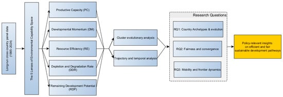
Figure 1. Analytical framework of environmental state-space evolution.

Temporal analysis is conducted using distance to the ideal, defined as the maximum score in each of the five capability dimensions. Trajectories are characterized in terms of capability driven improvement, permanent migration, and oscillation. Annual change is examined conditional on initial distance to evaluate catch up processes and frontier slowdowns, thereby addressing RQ2. By stratifying trajectories by archetype and region, the role of starting distance and regional context in mobility, permanence, and reversals is assessed, addressing RQ3. Figure 1 summarizes the analytical flow from lenses to archetypes to trajectories and motivates the policy interpretation.

3.2. The 5-Dimensional Environmental Lenses

The capability approach prioritizes the evaluation of systems based on their achievements rather than merely the quantity of inputs they possess (Sen, 1999). When applied to sustainability, this approach shifts attention to structural conditions. The comparative ability of countries to transform resources into sustainable environmental and developmental outcomes is then emphasized. This study adopts this perspective through five lenses, emphasizing capability as the foundation for comparison and interpretation, rather than relying solely on inputs.

• Productive capacity (PC)

The PC lens captures a nation’s productive base to generate prosperity through the effective use of resources. Consistent with Sen’s capability approach, it reflects both resource stocks and the ability to convert them into welfare enhancing outcomes (Sen, 1999). To move beyond income ranking, productive potential is represented using a Cobb–Douglas structure linking output to capital, labor, and human capital. Within the five-lens system, PC is interpreted as an enabling means dimension rather than environmental performance itself. High PC can coexist with low RE or high depletion burdens when production remains carbon and resource intensive. Intuitively, higher PC indicates a larger productive base per person and greater capacity to finance transition investments and absorb adjustment costs. Lower PC implies tighter structural constraints, so environmental improvements may face stronger trade-offs with growth and basic development needs.

• Developmental momentum (DM)

The DM lens captures output growth beyond what can be explained by changes in capital, labor, and energy. High momentum indicates that output grows faster than the input bundle, which is consistent with innovation, upgrading, and efficiency improvement. Low or negative momentum indicates weaker productivity dynamics. DM is operationalized using growth accounting and endogenous growth logic as total factor productivity, measured by the Solow residual after accounting for capital, labor, and energy inputs (Solow, 1956; Romer, 1990). DM is interpreted as a dynamic capability rather than a fixed endowment. Intuitively, higher DM indicates that the input bundle is being used more effectively over time. Persistently low or negative DM indicates weaker upgrading dynamics, so emissions reductions may require more targeted transition policies.

• Resource efficiency (RE)

The RE lens captures how much output is produced for a given level of energy use and greenhouse gas emissions. It aligns with Kaya style decompositions and eco efficiency perspectives that emphasize reducing pressure per unit of output as a core transition mechanism (Kaya, 1990; OECD, 2011). RE therefore reflects technical and structural drivers of decoupling, including technology, sectoral composition, and energy system efficiency. High RE indicates that substantial output is produced with relatively low energy reliance and emissions intensity. Low RE indicates energy intensive and carbon intensive production structures. In practical terms, RE distinguishes whether environmental progress is achieved through “doing more with less” rather than through slower economic activity. A lower RE implies that comparable growth tends to translate into higher pressure unless the production mix and energy supply are transformed.

• Resource depletion and degradation ratio (DDR)

The DDR lens reflects the income share associated with natural capital depletion and environmental degradation and can be interpreted as a development drag. In the raw World Bank series, a higher burden share indicates that a larger fraction of income is absorbed by depletion and damages, implying stronger erosion of future capacity. For consistency across the five lenses, the burden measure is inverted before scaling. Higher DDR in capability space therefore indicates lower erosion and a more sustainable position. The interpretation follows green accounting and genuine savings logic, where depletion and degradation reduce the asset base that supports long-run production and welfare. Intuitively, DDR captures whether current prosperity is being supported by running down natural capital. Higher DDR after inversion indicates that depletion and damage burdens are smaller relative to income, while lower DDR indicates stronger erosion pressures and higher risk that near term gains are achieved at the expense of future capacity.

• Remaining Development potential (RDP)

The RDP lens captures remaining development capacity within sustainability limits. A carbon constrained frontier is used, informed by planetary boundary and Paris Agreement perspectives (Rockström et al., 2009; Steffen et al., 2015; IPCC, 2022). RDP is expressed through per capita emissions relative to a carbon budget. Higher RDP indicates greater remaining emissions headroom, while lower RDP indicates proximity to the constraint. Within the five-lens framework, RDP is interpreted as a ceiling dimension that conditions feasibility and helps identify frontier proximity and permanence. In practical terms, RDP distinguishes between countries that remain comfortably below a per capita emissions guardrail and those operating close to, or above, that boundary. Lower RDP implies that further welfare gains must be achieved through faster decarbonization and efficiency improvement to avoid breaching the limit.

4. Methodology

The methodological framework is designed to provide an interpretable and time comparable representation of how countries evolve in a five-dimensional economic environmental capability space (Figure 2). First, lens definitions are specified mathematically and the resulting country–year scores are transformed to ensure comparability across lenses and years, with orientation set such that higher values consistently indicate stronger capability. Second, pooled k-means clustering is applied to the full country–year panel to identify stable archetypes over the study period using a single global set of centroids. Third, the resulting capability space is evaluated using distributional measures of attainment inequality (Gini and Palma), mobility diagnostics based on transition patterns and a five-year permanence rule, and distance-based metrics that quantify attainment, movement, and effectiveness relative to an ideal reference point. The ideal reference point is treated as an analytical benchmark that anchors distance and attainment comparisons and is not interpreted as a prescriptive policy target. Finally, robustness and sensitivity checks are conducted to assess whether the main inferences remain stable under plausible parameter and design perturbations.

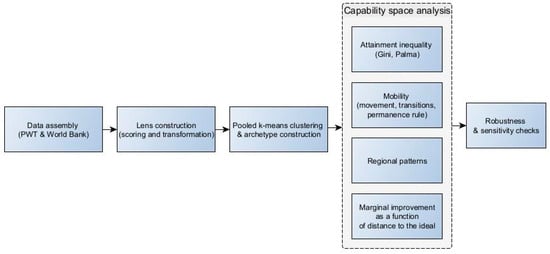
Figure 2. Methodological workflow for econo-environmental state-space evolution in five-lens capability space.

4.1. Data and Preprocessing

The empirical framework constructs a global country–year panel for 1995 to 2024. The panel is designed to support pooled clustering for archetype persistence (RQ1), fairness in attainment and frontier behavior (RQ2), and transition structure by archetype and region (RQ3). Data were sourced from two harmonized databases. The Penn World Table (Feenstra et al., 2015) provides macroeconomic quantities and factor inputs, while the World Development Indicators (World Bank, 2025) provide environmental and auxiliary series. Variable selection followed three criteria. Representativeness for the five lenses (PC, DM, RE, DDR, and RDP) was required, together with cross country coverage and statistical reliability. The final dataset included 118 countries. Definitions and data sources are reported in Table 2.

Table 2. Indicators used across five environmental performance lenses.

Dimensional Lens	Indicator Data
Productive Capacity (PC)	Main Data (PWT, 1995–2019): - Real GDP per capita—$GDPpc$ (USD 2017/person, output per person) - Capital per capita—$Kpc$ (USD 2017/person, physical capital stock per person) - Labor input per capita—$Lpc$ (labor participation, %) - Human Capital Index—$HCI$ (index 0–1, education-adjusted labor quality) Bridge indicators (WB, 2019–2024 extension): - Gross fixed capital formation per capita—$GFCFpc$ (USD 2015, proxy for capital investment) - Employment-to-population ratio—EPR (% of working-age population)
Developmental Momentum (DM)	Main Data: - Real GDP per capita—$GDPpc$ (USD 2017/person, output per person) (Feenstra et al., 2015) - Capital per capita—$Kpc$ (USD 2017/person, physical capital stock per person) (Feenstra et al., 2015) - Labor input per capita—$Lpc$ (labor participation, %) (Feenstra et al., 2015) - Energy use per capita—$Epc$ (kg oil equation/person, energy consumption intensity) Bridge indicators (WB, 2019–2024 extension): - Gross fixed capital formation per capita—$GFCFpc$ (USD 2015, proxy for capital investment) - Employment-to-population ratio—EPR (% of working-age population)
Resource Efficiency (RE)	GDP per unit of energy use—${\displaystyle \frac{GDP}{E}}$ (PPP $/kgoe, energy productivity) GDP per unit of GHG emissions—${\displaystyle \frac{GDP}{GHG}}$ (PPP $ per tCO2e, carbon productivity)
Depletion and Degradation Ratio (DDR)	Mineral depletion—$Dmrl$ (% of GNI, income-equivalent loss from mineral extraction) Energy depletion—$Dene$ (% of GNI, loss from fossil fuel extraction) Forest depletion—$Dfst$ (% of GNI, net forest rent losses)
Remaining Development Potential (RDP)	CO2 emissions per capita—$CO2epc$ (tCO2e/person, carbon pressure)
Notes: Unless otherwise stated, indicators were sourced from WDI (2024 release).

All series are expressed in per capita or intensity form when applicable. Population from the World Bank was used as the denominator to ensure cross country comparability. Short internal gaps were addressed using linear interpolation or short horizon imputation. Leading gaps were not filled to avoid artificial back projection. Lens construction follows Table 2. PC was derived from PWT factor-based quantities. DM was derived from multi-input productivity. RE was derived from output per unit energy use and emissions intensity. DDR was derived from adjusted net savings depletion shares. RDP was derived from per capita emissions relative to an equitable carbon budget threshold. The resulting balanced panel provides consistent inputs for subsequent steps.

4.2. Mathematical Specification of the Five Lenses

4.2.1. Productive Capacity

The computation of PC proceeds in two stages: first, establishing the base series using Penn World Tables data for the period 1995–2018; second, extending it to 2019–2024 through bridging with auxiliary indicators from the World Bank. This approach maximizes temporal coverage and captures longer run dynamics in environmental and developmental evolution. For the base period, PC is calibrated using a pooled log linear Cobb Douglas model with year fixed effects. GDP per capita is treated as the dependent variable, with capital, labor, and human capital as inputs:

$$\mathrm{l}\mathrm{n}GD{Ppc}_{i,t}=\alpha \ln {Kpc}_{ i,t}+\beta \ln {Lpc}_{i,t}+\gamma \ln HC{I}_{ i,t}+{\delta }_t+{\epsilon }_{i, t}$$

(1)

where i and t is the index of the country i at the study year t. Parameters $\alpha , \beta , \mathrm{a}\mathrm{n}\mathrm{d} \gamma$ are estimated elasticity of capital, labor, and human capital, ${\delta }_t$ denotes the year fixed effect, and ${\epsilon }_{i,t}$ represent the model noise. The calibrated parameters are then applied to the observed inputs to derive a productive capacity score. For 1995 to 2018, the raw score is defined as:

$$P{C}_{i,t}^{raw}=\mathrm{e}\mathrm{x}\mathrm{p}(\alpha \ln {Kpc}_{ i,t}+\beta \ln {Lpc}_{ i,t}+\gamma \ln HC{I}_{ i,t}+{\delta }_t)$$

(2)

Capital $Kpc$ is proxied using WB $GFCFpc$ and $Lpc$ is proxied using the $EPR$. Both indicators are then level-aligned to the PWT series using country-specific scaling factors derived from the 2015–2019 overlap period. HCI is assumed constant at its 2019 value.

$$\begin{gathered} s_{K,i}=media{n}_{t\in T}\left({\displaystyle \frac{{Kpc}_{i,t}}{GFC{Fpc}_{ i,t}}}\right), s_{L,i}=media{n}_{t\in T}\left({\displaystyle \frac{{Lpc}_{ i,t}}{{EPR}_{i,t}}}\right) \\ {K}_{i,t}^{tail}=s_{K,i}GFC{Fpc}_{i,t}, L_{ i,t}^{tail}=s_{L,i}EP{R}_{i,t}, HC{I}_{ i,t}^{tail}=HC{I}_{i,2019} \end{gathered}$$

(3)

The calibrated Cobb–Douglas elasticities are subsequently applied to these aligned inputs, and the PC score for 2020–2024 is obtained as the exponential of the fitted log specification:

$$P{C}_{i,t}^{tail}=\mathrm{e}\mathrm{x}\mathrm{p}(\alpha \ln {Kpc}_{ i,t}^{tail}+\beta \ln {Lpc}_{i,t}^{tail}+\gamma \ln HC{I}_{i,2019}+{\delta }_{ 2019})$$

(4)

4.2.2. Development Momentum

This lens computes total factor productivity growth as a Solow residual. A smoothing filter is then applied, which assigns 70% weight to the current year signal and 30% weight to the lagged signal. This specification reflects continuity in development processes, where productivity outcomes are shaped by both current conditions and momentum carried over from the recent past. DM is defined as:

$$D{M}_{ i,t}^{raw}=\lambda g_{i,t}^{TFP}+\left(1-\lambda \right)\rho g_{i,t-1}^{TFP}$$

(5)

Here, $\lambda$ = 0.7, so DM places greater weight on contemporaneous TFP growth, while the lagged term is dampened by $\rho =0.5$. The TFP residual is defined as:

$$g_{i,t}^{TFP}=g_{i,t}^{GDP}-{\theta }_K{g}_{i,t}^K-{\theta }_L{g}_{i,t}^L-{\theta }_E{g}_{i,t}^E$$

(6)

The coefficients ${\theta }_K, { \theta }_L$, and ${\theta }_E$ denote fixed factor elasticities with values of 0.35, 0.60, and 0.05, respectively, reflecting long-run averages of capital, labor, and energy shares. This convention follows the growth accounting tradition (Solow, 1956; Berndt & Wood, 1975) and ensures comparability of TFP residuals across countries and years. The notations $g_{i,t}^{GDP}, { g}_{i,t}^K, g_{i,t}^L,\mathrm{a}\mathrm{n}\mathrm{d} g_{i,t}^E$ denote the log-difference growth rates of $GDP, K, L,$ and $E$, serving as the observable input components in the decomposition. Capital stock K is estimated by using the Perpetual Inventory Method (PIM):

$$K_{i,t}=\left(1-\delta \right)K_{i,t-1}+GFC{Fpc}_{i, t}, K_{i,0}={\displaystyle \frac{GFC{Fpc}_{i,0}}{\delta +g}}$$

(7)

Here, δ = 0.05 and g = 0.03 represent the depreciation rate and the long-run growth assumption, respectively, both of which fall within the conventional ranges widely employed in growth accounting and PIM applications in the empirical literature.

For consistency with PC, the DM series for 2020–2024 is extended using the same bridging procedure described above, aligning World Bank auxiliary indicators with the PWT base through country-specific scaling over the 2015–2019 overlap period.

4.2.3. Resource Efficiency

The resource efficiency (RE) lens builds on the Kaya identity (Kaya, 1990), which decomposes emissions into activity, structure, energy intensity, and carbon intensity. We adopt its inverse perspective, emphasizing efficiency: higher output per unit of resource use or emissions reflects greater sustainability. Two sub-indices are therefore considered:

$$C_{i,t}^E={\displaystyle \frac{{GDP}_{i,t}}{E_{i,t}}}, GDP per unit of energy use$$

(8)

$$G_{i,t}^{GHG}={\displaystyle \frac{{GDP}_{i,t}}{GH{G}_{i,t}}}, GDP per unit of greenhouse gas emisison,$$

(9)

Here, $E_{i,t}$ denotes energy use and $GH{G}_{i,t}$ denotes total greenhouse gases emissions. Because these components are expressed in different units, logged values year-wise normalization is applied to ensure scale invariance and allow aggregation. For country i in year t, each component is log-transformed and standardized:

$${zscore}_{i,t}^E={\displaystyle \frac{ln{C}_{i, t}^E-{\mu }_t^E}{{\sigma }_t^E}}, {zscore}_{i,t}^{GHG}={\displaystyle \frac{ln{C}_{i, t}^{GHG}-{\mu }_t^{GHG}}{{\sigma }_t^{GHG}}}$$

(10)

where $\mu \mathrm{a}\mathrm{n}\mathrm{d} \sigma$ denotes the within year mean and standard deviation of the logged component. The composite RE lens is then computed as:

$$R{E}_{i,t}^{raw}=w_E{zscore}_{i,t}^E+w_{GHG}{zscore}_{i.t}^{GHG}$$

(11)

where w_E = 0.5 and w_GHG = 0.5, equal weights are applied to the two components.

4.2.4. Degradation and Depletion Ratio

Grounded in green accounting/genuine-savings theory, DDR uses World Bank adjusted-savings data. Each component is expressed as % of GNI and covers mineral, energy, and net forest depletion (country i, year t):

$$DD{R}_{i,t}^{raw}={Dmrl}_{i,t}+{Dene}_{i,t}+{Dfst}_{ i,t}$$

(12)

A higher score $DD{R}_{ i,t}^{raw}$ signals a stronger development drag. Today’s output is achieved by depleting tomorrow’s productive base. DDR complements the other lenses by making the intertemporal cost explicit. For cross-lens comparability, this lens is re-oriented during the common scaling step, so that higher values in the capability space indicate lower depletion and degradation.

4.2.5. Remaining Development Potential

RDP was operationalized as an environmental headroom lens: country–year conditions were compared against benchmarks to assess safe room for development versus environmental cost risks. The benchmark focuses on per capita CO₂ emissions, following literature emphasizing carbon budget as the critical constraint for intergenerational sustainability. A threshold of 1.9 tCO₂e per person per year was adopted as a Paris-consistent reference under equitable sharing of the 1.5 °C carbon budget (Chancel, 2022; IPCC, 2022). The headroom function captures whether countries operate within this per capita limit, with values declining toward zero as emissions exceed the benchmark.

$$RD{P}_{ i,t}^{raw}=\left\{\begin{array}{cc}\hfill 0,& CO{2epc}_{i,t}\ge 1.9\hfill \\ \hfill 1-\left({\displaystyle \frac{CO{2epc}_{i,t}}{1.9}}\right),& CO{2epc}_{i,t}<1.9\hfill \end{array}\right.$$

(13)

4.3. Archetype Construction and Clustering Procedure

The research questions are addressed by recovering stable archetypes from the five-lens capability space using pooled k-means (MacQueen, 1967). Archetype membership provides a parsimonious description of country–year outcomes and is used as an organizing structure for the fairness and mobility analyses. RQ1 is operationalized by evaluating cluster separation, stability, and centroid profiles over time.

To ensure comparability across lenses and years, preprocessing was applied to each country–year lens series $(P{C}_{it}^{raw}, {DM}_{it}^{raw}, {RE}_{it}^{raw}, {DDR}_{it}^{raw}, {RDP}_{it}^{raw})$. Interior and tail imputation was used when coverage was sufficient, while short series with insufficient coverage were excluded. Each lens was standardized using z-scores and then compressed using a hyperbolic tangent transform with τ = 2, so that the mid distribution was preserved while extreme values were dampened. The compressed values were linearly rescaled to the interval [−1, 1]. A symmetric [−1, 1] scale was preferred because it supports interpretation in relative terms, where negative values indicate below typical performance and positive values indicate above typical performance. This also avoids the interpretation risk of a [0, 1] scale, where values near zero can be read as an absolute absence of capability. Lenses were oriented for better performance values; DDR was sign-inverted before scaling. The resulting observation for country i in year t is the five-dimensional vector:

$$z_{i,t}=\left(P{C}_{i,t}, D{M}_{i,t}, R{E}_{i,t}, DD{R}_{i,t}, RD{P}_{i,t}\right)\in {\mathbb{R}}^5$$

(14)

A single global clustering solution was estimated on the pooled panel {z_i,t} so that one set of centroids represents time invariant archetypes. This design was adopted to maintain comparability across decades under fixed archetype definitions. When clustering is performed independently for each year, label alignment across time is not ensured. Observed movement can then be induced by changes in cluster definitions rather than by changes in country position. Within year clustering can facilitate clearer cross-sectional comparison within a given year. However, the resulting clusters are not anchored to time invariant archetypes, so evolutionary inference across the full period is not supported.

Clustering was then performed using k-means on the pooled panel in the standardized capability space. A centroid based method was preferred because archetypes are represented directly by centroids that can be profiled and compared across time. K-means was therefore selected for interpretability and for compatibility with Euclidean distance after standardization. K-means partitions the pooled panel into K clusters by minimizing the within cluster sum of squared Euclidean distances. The algorithm proceeds iteratively. Observations are assigned to the nearest centroid, and centroids are updated to the mean of their assigned observations until assignments stabilize. The formal k-means objective is given below:

$${\displaystyle \genfrac{}{}{0pt}{}{min}{{\left\{{\mu }_k\right\}}_{k=1}^K, {\left\{C_k\right\}}_{k=1}^K}}\sum _{k=1}^K\sum _{z\in C_k}{\left|\left|z-{\mu }_k\right|\right|}_2^2$$

(15)

where ${\mu }_k$is the centroid of the cluster $C_k$. The algorithm then runs assignment and update logic until achieving convergence,

$$z_{i,t}\to C_k if k=\arg {\displaystyle \genfrac{}{}{0pt}{}{min}{j=1, \dots , K}}{\left|\left|z_{i,t}-{\mu }_j\right|\right|}_2,$$

(16)

$${\mu }_k\leftarrow {\displaystyle \frac{1}{\left|C_k\right|}}\sum _{z\in C_k}z$$

(17)

Multiple criteria were applied for diagnostic evaluation of robustness and for selection of the cluster number. The elbow method was used to examine within cluster variance across candidate values of cluster size K, and silhouette scores were used to assess cohesion and separation. Multiple random initializations were performed, and the solution with the lowest within cluster sum of squares was retained. In addition, cluster stability was evaluated using the adjusted Rand index (ARI) across repeated initializations and repeated runs. Together, these diagnostics were used to support the retained K choice and to confirm that partitions were well distinguished and stable. For diagnostic evaluation, K was screened over K = 2 to 10.

Clusters represent archetypes of the country’s environmental performance state, thus cluster labelling needs to be arranged to improve interpretability. Relabeling is done by composite performance over the 5 lenses (l):

$$s_k={\displaystyle \frac{1}{5}}\sum _{l=1}^5{\mu }_{k, l}.$$

(18)

Cluster 1 thus represents the lowest $s_k$ (weakest state) and cluster K will read as the group with highest $s_k$ (strongest cluster).

We applied principal component analysis (PCA) to the scaled panel dataset for visualizing the five-lens clustering results. PCA served only as a visualization aid, projecting high-dimensional data onto two principal axes. We retained the first two components (PC1 and PC2), which capture most variance in lens scores, and report their explained variance ratios. This projection enables two-dimensional plots showing cluster archetypes and temporal migration paths, while maintaining comparability of clusters in the original five-lens space.

4.4. Fairness Analysis

This subsection addresses Research Question 2 (RQ2). Cross-sectional inequality in environmental capability is evaluated over 1995–2024 to assess whether it is minimal and gradually decreasing. It also examines the relationship between fairness and frontier deceleration as the distance diminishes. Annually, each country’s attainment is calculated based on its proximity to the ideal point $I=(1, 1, 1, 1, 1)$ in the five-dimensional capability space. The ideal point represents a coordinate reference for distance-based measurement in the normalized capability space. It is not intended as a prescriptive policy target, but as a device for comparing relative proximity and changes over time under a common scale. Fairness is assessed across the cross-section of attainment using the Gini index and the Palma ratio (top 10% vs. bottom 40%). To link fairness with frontier behavior, distance-conditioned improvement is analyzed through distance to the ideal (DDI) gradients and effectiveness near small initial distances.

For each country i at the year t, the Euclidean distance $d_{i,t}$ to the ideal can be written as:

$$d_{i,t}={\left|\left|\mathsf{{\rm I}}-s_{i,t}\right|\right|}_2=\sqrt{\sum _{k\in \{PC, DM, RE, DDR, RDP)}{\left(1-z_{i,t}^k\right)}^2}$$

(19)

For distributional analysis the metric was inverted to an attainment scale where larger values indicate better performance and support is nonnegative. This inversion aids Gini construction since the index use nonnegative quantities ordered low to high. With a higher-is-better orientation, the Lorenz curve ranking corresponds to increasing proximity to the ideal, and inequality levels represent proximity concentration among countries yearly.

Formally the maximum possible distance $DMAX= \sqrt{20}$, attainment was defined as:

$$A_{i, t}=DMAX-d_{i,t}\in \left[0, DMAX\right]$$

(20)

The Gini index at the year t is thus can be computed as:

$$Gini={\displaystyle \frac{1}{2N_t^2\overline{A_t}}} \sum _{i=1}^{N_t}\sum _{j=1}^{N_t}|A_{ i, t}-A_{j,t}|$$

(21)

where $N_t$ and ${\overline{A}}_t$ denotes the number of countries observed and cross-sectional mean attainment in the year t. The Gini index measure summarizes dispersion over the entire distribution and equals twice the area between the Lorenz curve of attainment and the 45-degree equality line (Gini, 1912). Lower Gini values indicate higher fairness in that year, meaning that countries are more similarly distributed in their proximity to the ideal.

The Palma ratio which indicates the ratio of the upper and lower tail of the data are given by:

$$Palm{a}_t={\displaystyle \frac{A_t^{top10}}{A_t^{top40}}}$$

(22)

where $A_t^{top10} \mathrm{a}\mathrm{n}\mathrm{d} A_t^{top40}$are mean attainment of the top 10% and bottom 40% countries of the year t. This index focuses on the tails and captures whether gains in proximity to the ideal are concentrated among the best performers relative to the weakest segment (Palma, 2011). A larger value indicates that the upper tail is pulling away from the lower tail even if the middle of the distribution is relatively stable.

Higher Gini or Palma values indicate advantages concentrated among certain countries, while lower values suggest more equitable distribution near the ideal.

4.5. Temporal Analysis

This subsection provides a system view of how countries navigate capability space over 1995–2024, linked to four archetypes. RQ1 is addressed by tracking archetype persistence through cluster shares and centroid paths. RQ3 is addressed by summarizing mobility using transition probabilities, permanence (no move back for five years), and boundary reversals, with regional context. These temporal diagnostics, alongside fairness results, clarify whether change arises from tightening within clusters or reallocation across clusters.

The five panels of the analysis report: (a) annual archetype shares, (b) mean within cluster distance to centroid by archetype, (c) total annual movement in capability space measured by step length, (d) annual migration counts (up and down), and (e) permanent upgrades and downgrades under the five-year rule.

Within cluster distance (W) is measured as the mean Euclidean distance of members to the year specific centroid ${\mu }_{c,t}$. The measure is given by:

$$W_{c,t}={\displaystyle \frac{1}{n_{c,t}}}\sum _{i\in c}{\left|\left|z_{i,t}-{\mu }_{c,t}\right|\right|}_2$$

(23)

A declining trajectory indicates tightening dispersion and greater internal cohesion within the archetype, whereas an increasing trajectory suggests fragmentation or boundary churn; this indicator complements migration counts by testing whether compositional shifts are accompanied by genuine consolidation inside clusters.

Movement within capability space is measured as annual Euclidean step lengths in five-dimensional state space:

$$M_t=\mathsf{\Sigma }{\left|\left|\Delta z_{i,t}\right|\right|}_2$$

(24)

where $z_{i,t}$ denotes the vector of standardized lens scores for country i in year t.

Annual migration counts are computed to quantify upward and downward shifts in cluster rank between consecutive years.

Finally, a permanence metric was introduced to distinguish sustained migration from short run switching. A migration was classified as permanent when a country did not return to its origin cluster within five subsequent years. A five-year horizon was selected as a pragmatic compromise. Shorter windows are more sensitive to oscillatory reassignment around cluster boundaries. Much longer windows reduce the number of observable permanent events within the 1995 to 2024 sample and can understate durable change. The forward-looking permanence functions, $P_t^{up}, P_t^{down}$ capture the frequency of permanent upward and downward migrations in each year. In other words, once a shift in cluster rank persists for at least a five-year horizon, it is recorded as a durable transition. Sensitivity of permanence classification to the chosen horizon is acknowledged, and the five-year rule is interpreted as a conservative filter for sustained mobility.

4.6. Dynamic Distance Improvement (DDI) Analysis

DDI quantifies annual progress toward the ideal, capturing substantive advancement. By relating DDI to the starting distance from the ideal, catch up and frontier slowdowns can be identified. This addresses RQ2 beyond cluster membership. Examining DDI by archetype and by starting distance also helps distinguish compositional shifts from genuine convergence. When combined with transition results, the analysis links distance, context, and mobility to address RQ3. In this way, heterogeneity that is hidden in aggregate trends is made visible, while interpretation remains anchored to the same ideal reference point. The one-year improvement in proximity to ideal is given as:

$$DD{I}_{i,t}=A_{i,t}-A_{i,t-1}=d_{i,t-1}-d_{i,t}$$

(25)

Hence $DD{I}_{i,t}>0$ indicates movement closer to the ideal in year t for country i. Profiles of $DD{I}_{i,t}$ were evaluated as a function of starting distance of $d_{i,t-1}$ using binned cross-sectional means to summarize distance-conditioned behavior.

Furthermore, the effectiveness of movement measures how much of the annual movement in the capability space is converted into useful progress toward the ideal state. It is defined by:

$$Ef{f}_{i,t}=\left\{\begin{array}{c}{\displaystyle \frac{DD{I}_{i, t}}{L_{i,t}}}, L_{i,t}>0, \\ 0, L_{i,t}=0\end{array}\right.$$

(26)

where $L_{i,t}$is given as the total distance moved in a year:

$$L_{i,t}={\left|\left|z_{i,t}-z_{i,t-1}\right|\right|}_2$$

(27)

Analyzing effectiveness based on distance and clustering provides insights into whether proximate or distant countries from the ideal effectively translate potential into progress. This analysis distinguishes between efficient convergence and lateral movements, thereby refining mechanisms addressed in RQ3.

4.7. Sensitivity Analysis

As an additional robustness check, sensitivity tests were conducted for both the lens weighting scheme and the RDP per capita CO₂e emissions (tCO₂e) threshold. The scoring and clustering framework was re-run under one at a time-perturbations around the baseline specification, including the lens weighting and ±20% variation in the emission threshold used to operationalize remaining development potential. Clustering stability was evaluated using the ARI relative to the baseline solution. Complementary diagnostics were also inspected, including changes in cluster sizes, shifts in transition patterns, and distributional changes in affected lens scores across countries. These tests were used to assess whether the main clustering structure and mobility conclusions are preserved under plausible parameter uncertainty.

4.8. Generative AI Usage

Generative AI tools were used for limited language editing and routine coding assistance. All research design, analysis, and interpretation were conducted by the authors, who take full responsibility for the manuscript.

5. Results and Discussion

5.1. Cluster Formation and Archetypes

The diagnostic analysis reveals a discernible trade-off among fit, separation, and stability. The elbow curve in Figure 3 panel (a) shows rapidly diminishing returns beyond k = 4. This suggests that additional clusters contribute minimally to within cluster improvement. The silhouette scores in panel (b) peak around k = 3–4 and then decline, indicating weaker separation when k exceeds four. Stability across random seeds, measured by the ARI in panel (c), remains consistently high. However, the most robust and consistent stability is observed at k = 4, whereas larger k values yield lower minima and greater dispersion. Collectively, k = 4 emerges as a modest and stable choice. Internal cohesion and between-cluster separation are retained while over-partitioning is avoided.

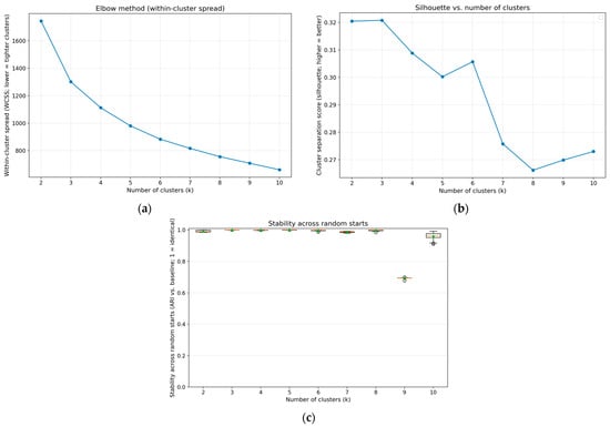
Figure 3. (a) Elbow of within cluster sum of squares; (b) silhouette score; (c) stability across seeds measured by adjusted Rand index (ARI). The boxes in panel (c) appear as thin lines for most k because the dispersion of ARI values is extremely small (ARI close to 1), indicating high stability across seeds. Together these diagnostics indicate k = 4 as a modest and stable choice.

The pooled PCA in Figure 4a shows a clear two-dimensional structure in the environmental capability space. PC1 explains 51.89% of the variance and PC2 explains 17.39%, for a combined 69.28%. As indicated by the axis notes, the positive side of PC1 aligns with higher PC, RE, and DDR, while the negative side aligns with higher RDP and DM. The positive side of PC2 aligns with higher PC and DM, while the negative side aligns with higher RE, DDR, and RDP. Four archetypes are visually distinct. C1 is concentrated in the upper, slightly left region, indicating a DM oriented profile with weaker DDR. C2 is positioned on the left, indicating relatively greater headroom with constrained capability. C3 lies near the center, slightly to the right and below, indicating an intermediate and broadly balanced profile. C4 is concentrated on the right, reflecting stronger capability with tighter headroom. The kernel density envelopes show limited overlap across clusters, which is consistent with standard validation guidance (Kaufman & Rousseeuw, 1990; Everitt et al., 2011).

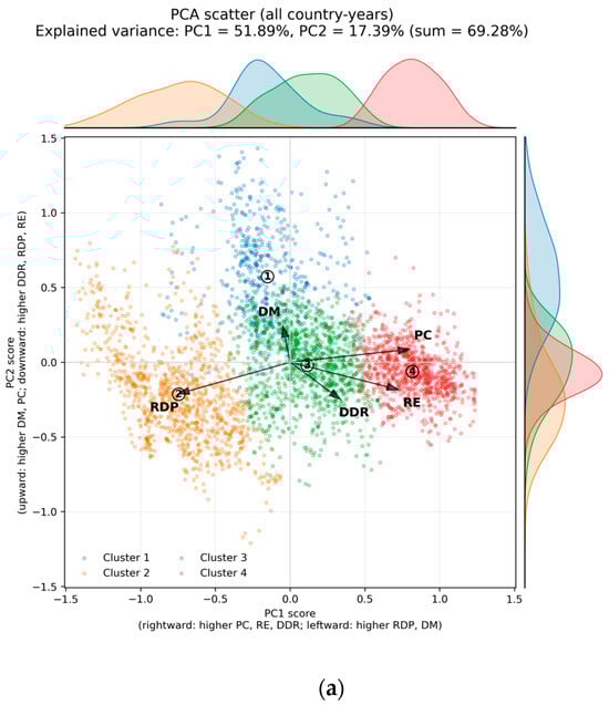
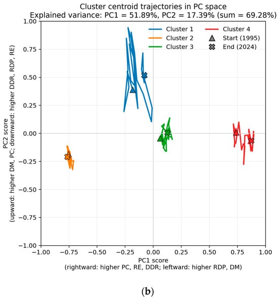
Figure 4. Environmental capability space. Percentages denote explained variance for Principal Component 1 and 2 (PC1 and PC2); axes show principal component scores. (a) PCA scatter of all country-years with k-means cluster labels in the two-dimensional PC1–PC2 plane, with marginal KDEs showing cluster-wise distributions of PC1 (top) and PC2 (right). Loading arrows indicate direction of increasing values for each lens, and arrow length reflects loading strength. A country–year has a higher value on a lens when it lies further in the arrow direction and a lower value when it lies opposite to it (e.g., C4 lies along PC arrow, indicating higher PC, whereas C1 lies opposite from it, indicating lower PC). (b) Cluster centroid trajectories in PC plane, 1995–2024. Each point denotes the annual cluster centroid, and movement reflects changes in the cluster’s average lens profile. Trajectories are short and do not cross; the partition is therefore stable.

The centroid trajectories over 1995 to 2024 remain separated, and crossings are not observed, which supports the stability of the cluster number k = 4 (Figure 4b). C1 shifts upward and slightly rightward, which is consistent with stronger DM alongside stronger PC. C2 remains compact in the lower left with only minimal movement. C3 remains close to the origin with a small drift. C4 shifts rightward and slightly downward despite already high capability, indicating further strengthening in RE and DDR, while headroom remains tight as reflected by opposite movement from RDP loadings.

The four archetypes can be read as distinct profiles in the five-lens capability space, as shown in Figure 5, and their concise interpretations are given below

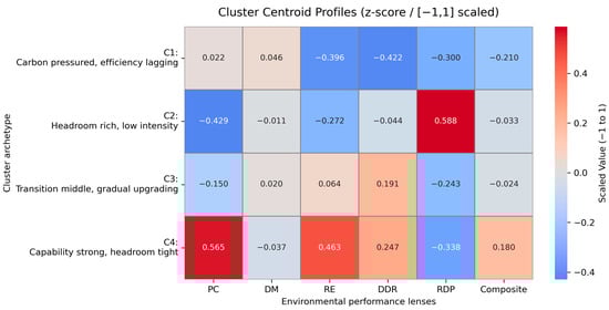
Figure 5. Four archetypes in five-lens environmental capability space. Cells report cluster centroid values. Positive values indicate above sample average performance on a lens, while negative values indicate below sample average performance. Composite column summarizes average lens profile for each archetype.

• Cluster 1—Carbon pressured, efficiency lagging

PC is 0.022 and DM is 0.046, while RE and DDR are negative at −0.396 and −0.422, and RDP is also negative at −0.300, which yields the lowest composite at −0.210. This profile is consistent with systems where resource efficiency and depletion burden reductions remain limited, and where carbon headroom is below average relative to peers.

• Cluster 2—Headroom rich, low intensity

PC is −0.429 and DM is −0.011, RE is −0.272, DDR is −0.044, and RDP is the highest at 0.588, which results in a near-zero composite at −0.033. This profile is consistent with low capacity and low efficiency at modest scale, with relatively high carbon headroom and limited depletion pressure, rather than a mature high-performance transition.

• Cluster 3—Transition middle, gradual upgrading

PC is −0.150 and DM is 0.020, while RE and DDR are mildly positive at 0.064 and 0.191, and RDP is −0.243, which yields a near-zero composite at −0.024. This suggests incremental upgrading with some efficiency and lower-erosion progress but without the capacity lift to move decisively rightward.

• Cluster 4—Capability strong, headroom tight

C is 0.565 and DM is −0.037, RE is 0.463 and DDR is 0.247, while RDP is negative at −0.338, which yields the highest composite at 0.180. This profile is consistent with high capability and efficiency, coupled with limited carbon headroom, which aligns with partial rather than absolute decoupling.

Overall, the PCA mapping delineates interpretable archetypal states that can be used as reference points for trajectory analysis and for the discussion of policy levers. Together with the stability diagnostics and the compact centroid trajectories, the k = 4 solution is supported as a modest and stable representation of country–year patterns over 1995 to 2024. In this way, RQ1 is addressed through an enduring set of archetypes that is suitable for subsequent mobility and convergence analysis.

5.2. Five-Dimensional Gini and Palma Ratio

The global perspective on fairness within the capability space is reflected in the inequality of attainment. Both indicators have remained low from 1995 to 2024, with a slight decline observed: the Gini coefficient fluctuates closely around approximately 0.10 with a minor negative trend, while the Palma ratio decreases from the mid-1.5 to the low-1.4. Since attainment measures the proximity to the capability ideal, low and gradually decreasing dispersion suggests a generally similar opportunity to reach the frontier and a modest convergence in capability. Although short-term oscillations are present, no structural break is visually discernible.

In practical terms, the low and gently declining Gini and Palma values suggest that attainment has not become more polarized into persistent leaders and laggards. This is consistent with a mild form of club convergence across the archetypes. C1 and C2 retain larger remaining headroom, so they have greater scope to reduce distance to the ideal when improvements occur. C4 is closer to the frontier and faces tighter headroom, so gains are expected to be smaller and reversals can be more visible. C3 occupies an intermediate position, where incremental improvements would be expected.

The joint behavior of the Gini and Palma indices suggests that the pattern is not confined to the extremes of the attainment distribution. When both measures remain low and decline gently, dispersion is implied to be narrowing across the upper tail, the middle, and the lower tail, rather than shifting only through changes among a few frontier cases. This pattern is consistent with transition mechanisms based on diffusion and incremental adoption, rather than abrupt redistribution (Markard et al., 2012; Renou-Maissant et al., 2022). A practical implication follows for the mobility analysis. If dispersion is already low, smaller gains would be expected near the frontier than farther from it, and occasional reversals may be more visible among high attainment cases. This distance conditioned asymmetry is examined using the DDI results. Figure 6 therefore supports RQ2 by documenting low and gently declining cross-sectional inequality in attainment, while the transition and DDI evidence is used to interpret mobility patterns (Section 5.5).

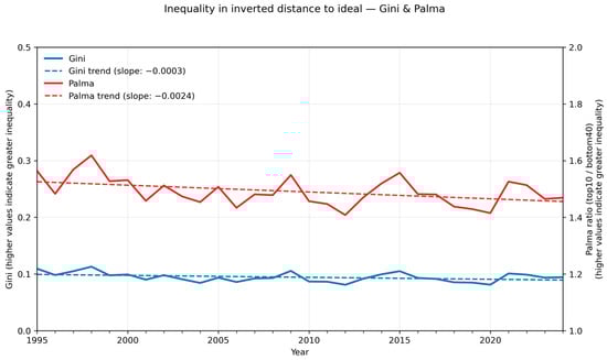
Figure 6. Five-dimensional Gini and Palma inequality indices with capability value measured from ideal state.

5.3. Cluster Dynamics and Temporal Analysis

Evidence on fairness indicates that opportunities are broadly comparable across nations. The temporal evidence is consistent with this pattern. Cluster shares change gradually, within cluster distances to centroids tend to decline, and mobility is limited, with permanent upward moves exceeding permanent downward moves. Given the low dispersion, attention is shifted from static levels to movement over time, including its direction and persistence. Figure 7 therefore summarizes share dynamics, cohesion around centroids, and permanent transitions.

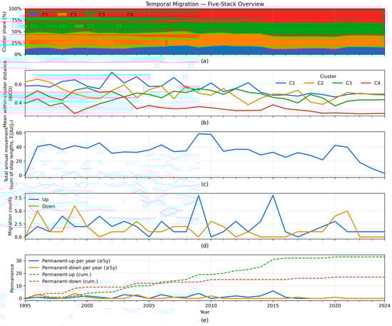
Figure 7. Temporal migration in environmental capability space, 1995–2024. (a) Cluster composition; (b) mean distance to cluster centroids; (c) total annual step length; (d) counts of upward and downward moves; (e) cumulative permanence under five-year no-reversal rule.

Each panel read as follows:

Figure 7a: How stable shares with a gradual expansion of C4 and C3 remain broadly stable, while C2 contracts and C1 remains small. The drift toward C4 indicates that more countries locate in the high capability archetype over time, suggesting selective upgrading within persistent clubs rather than frequent tier switching.

Figure 7b: Mean distance to centroid (WCD). All clusters exhibit gentle declines in within cluster distance, with C4 the tightest and C2–C3 narrowing over time. This indicates growing cohesion inside clubs (“tightening cores”), reinforcing that the four archetypes act as stable attractors rather than fragile partitions.

Figure 7c: Total movement |Δc|. System-wide mobility peaks around the late 2000s and then trends downward, suggesting that the post-crisis decade saw consolidation rather than churn. Fewer countries change club each year as the capability landscape settles.

Figure 7d: Up vs. down transitions. Upward moves generally outnumber downward moves in most years, with episodic spikes rather than sustained bursts. Net mobility is therefore positive but incremental.

Figure 7e: Permanence (≥5-year, no-reversal rule). Cumulative permanent-up rises steadily and far exceeds permanent-down, while annual permanence events become sparse toward the end of the window. Upgrades tend to “stick,” which aligns with the tightening WCD and stable shares.

Across panels, the capability clusters are shown to be durable and dispersion is shown to be low. Progress is expressed through gradual improvements that consolidate over time. This pattern is consistent with tempered club convergence, in which most country-years remain within clusters and selective upgrading into C4 occurs with few reversals (Eleftheriou et al., 2024; Renou-Maissant et al., 2022). These results support RQ1 by confirming persistent archetypes. RQ2 is supported by the low and gently declining inequality in attainment, which implies limited polarization and smaller gains near the frontier. RQ3 is informed by constrained mobility, where permanent upward moves exceed permanent downward moves. The permanence metric separates sustained transitions from short run fluctuations. It supports the interpretation that capability change is driven by long cycle technological and managerial shifts.

Figure 8 is strongly diagonal, which indicates high year to year persistence and limited mobility. Upgrading is observed, but it occurs selectively. Most upward moves occur from C1 to C3 and from C3 to C4, while direct moves into C4 are rare. By contrast, movement across the C2 to C3 boundary is more often bidirectional, which suggests that many country-years lie near a threshold where small changes can shift cluster membership. Exits from C4 are uncommon, which is consistent with consolidation at high capability. These patterns support RQ3 by indicating tempered club convergence and multiple steady states (Eleftheriou et al., 2024; Renou-Maissant et al., 2022).

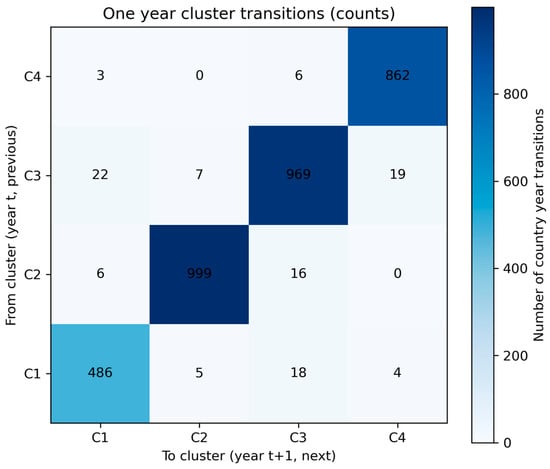
Figure 8. Global one-step transition matrix, pooled over all countries and consecutive year pairs (1995→1996 to 2023→2024). Rows indicate origin cluster at year t and columns indicate destination cluster at year t + 1; diagonal cells represent persistence.

Overall, the temporal evidence points to difficult class mobility and tempered club convergence. Low and gently declining inequality, strong diagonal persistence with only selective upgrading, and distance-conditioned improvement profiles together answer RQ3: capabilities are sticky, movement is stepwise, and durable gains accumulate gradually.

5.4. Dynamics Evolution of Countries and Region

The temporal analysis shows a stable landscape with limited class mobility and convergence in capability. This pattern is consistent with path-dependent accumulation. To examine these mechanisms regionally and identify areas of boundary stability, trajectories are analyzed by region. The regional analysis is used to detect variation at archetype boundaries and to link movement dynamics to capability advancement opportunities. This analysis supports RQ3 by examining club convergence under varied conditions. It is also aligned with evidence of multiple steady states across country groups (Eleftheriou et al., 2024; Renou-Maissant et al., 2022).

The regional pattern of ASEAN, East & Central Asia, and South Asia (Figure 9) remains characterized by stability with selective upgrading. Indonesia shows early oscillation between C2 and C3, followed by a brief mid period dip into C1, and then consolidation in C3 in the later years. Vietnam remains in C2 for most of the earlier period, exhibits a short C1 episode, and subsequently shifts into C3 and remains there. Singapore moves from C3 into C4 by the late 1990s and stays in C4 thereafter, indicating durable frontier positioning. The Philippines is predominantly in C2 and transitions to C3 only in the final segment of the window. Thailand is consistently assigned to C3 with no evident tier switching, while Myanmar remains consistently in C2. Malaysia and Brunei Darussalam remain largely in C1, with only brief deviations. Overall, mobility is concentrated in stepwise movement along the C2 to C3 corridor, while sustained C4 membership is restricted to Singapore. East and Central Asia shows a two-tier structure. Japan and the Republic of Korea anchor C4, while China is mainly C3 with temporary dips before reconsolidation. Kazakhstan and Mongolia remain persistently in C1, and Armenia steps from C2 to C3 and stabilizes. South Asia is C2 dominant with selective upgrades. India shifts from C2 to C3 around the early 2010s and then remains in C3, while Sri Lanka shifts from C2 to C3 and consolidates after a short transitional interruption. The Maldives remains largely in C3 but shows a brief C4 episode around 2020. Bangladesh, Nepal, and Pakistan remain persistently in C2. Oceania shows stability: Australia and New Zealand remain in the frontier archetype (C4), while Fiji maintains a mid–high capability position (C3).

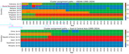
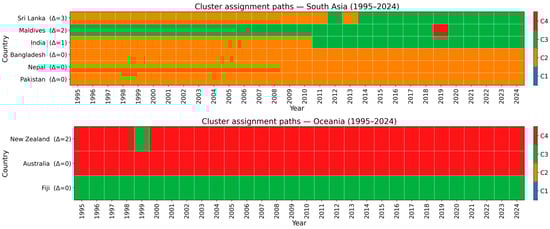
Figure 9. Country archetype evolution for ASEAN, East and Central Asia, South Asia, and Oceania (Δ = cluster transition counts).

The common pattern is tempered club convergence. Durable membership is observed alongside stepwise catch-up through the C2→C3 corridor, while direct moves to C4 remain rare. Boundary churn is concentrated in transitional cases. These patterns are consistent with gradual capability accumulation and uneven adjustment documented in distribution dynamics and transition studies (Eleftheriou et al., 2024; Renou-Maissant et al., 2022).

Throughout Europe, a bifurcated pattern exists (Figure 10). Eastern Europe exhibits stepwise upgrading that is primarily expressed as a C3 to C4 shift, with timing that differs across countries. Slovenia and the Czech Republic are anchored in C4 throughout the period, indicating consistently high capability. A first wave of convergence is visible in the 2000s, where Cyprus, Croatia, Hungary, Latvia, Lithuania, and Slovakia shift from C3 into C4, then remain consolidated. Poland and Romania follow as late movers, remaining largely in C3 for most of the sample and only entering C4 in the 2020s, which indicates delayed but eventual consolidation rather than early convergence. Albania shows an early transition from C2 into C3 and then remains stable in C3, while Bulgaria is largely persistent in C3 without a clear consolidation into C4 within the plotted window. By contrast, the Russian Federation and Ukraine remain persistently in C1, reflecting durable low capability membership in this representation. Western Europe is fully anchored in C4 from 1995 to 2024, indicating persistently high capability with negligible club switching. European integration enables upward mobility, while Western Europe’s stability reflects path dependence at high capability, reinforcing RQ3.

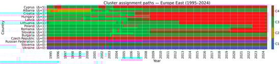
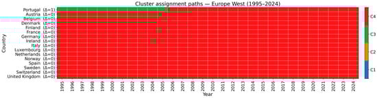
Figure 10. Country archetype evolution for Eastern and Western Europe (Δ = cluster transition counts).

North America shows stability (Figure 11): The US and Canada remain in the frontier archetype (C4), while Mexico maintains a mid-high capability position (C3). This aligns with path-dependent capability accumulation and “frontier lock-in,” where mature infrastructures yield limited class mobility (Dosi & Nelson, 2010; Markard et al., 2012). Latin America and the Caribbean show a club-based pattern (Figure 11). Several larger and more diversified economies remain predominantly in C3 (for example Argentina, Brazil, Colombia, Costa Rica, the Dominican Republic, and Uruguay), while structurally constrained cases persist in C2 (for example Haiti, Honduras, and Nicaragua). Mobility is mostly stepwise, occurring through C2→C3 upgrading (El Salvador and Paraguay) and C3→C4 transitions (Panama and Barbados). Mobility is mostly stepwise, occurring through C2→C3 upgrading and, in fewer cases, C3→C4 transitions, while oscillation is observed in Chile, Ecuador, Guatemala, Belize, and Bolivia. Trinidad and Tobago is an outlier that remains stably in C4. While North America shows minimal class mobility, Latin America provides regional volatility and some permanent upgrades—reflecting slow capability development and uneven reforms noted in sustainability-transition literature. Figure 11 show the transition of the regions.

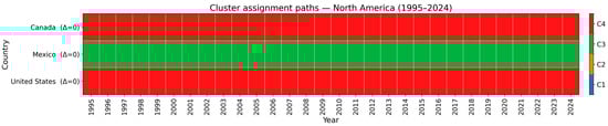
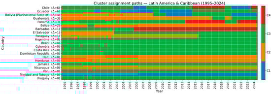
Figure 11. Country archetype evolution for North America, Latin America, and Caribbean (Δ = cluster transition counts).

The Middle East and North Africa display persistent stratification (Figure 12). Israel remains anchored in C4, while Turkey, Morocco, Jordan, and Tunisia are stably positioned in C3. A resource rich C1 group persists with limited mobility, including Iran, Iraq, Algeria, Bahrain, and largely Kuwait. Yemen remains in C2 throughout. Qatar exhibits episodic upgrading into C4 in the later years, whereas Egypt alternates between C1 and C3 and consolidates in C3 by the end of the window. Overall, mobility is selective and concentrated in a small number of cases, which is consistent with path-dependent capability accumulation in resource-oriented systems (Dosi & Nelson, 2010; Markard et al., 2012).

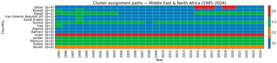
Figure 12. Country archetype evolution for Middle East and North Africa (Δ = cluster transition counts).

The region of Sub-Saharan Africa (Figure 13) is dominated by long spells in C2. This pattern indicates constrained capability with limited transitions. A few durable C3 placements are observed, for example in Mauritius, Botswana, and Namibia. Sporadic oscillations are observed in a small set of cases, notably Congo, South Africa, and Angola, which move between C1, C2, and C3 across sub-periods. Resource intensive enclave economies display extended C1 or C2 plateaus. Overall, cross cluster mobility remains scarce and no C4 placements are observed. Gabon remains stably in C1, while Congo exhibits the most pronounced switching, which is consistent with volatile resource linked trajectories. This pattern accords with the literature on capability bottlenecks and incremental transitions. Institutional and infrastructural constraints are emphasized as factors that slow accumulation and limit the scope for rapid decoupling from environmental pressure (Dosi & Nelson, 2010; Markard et al., 2012).

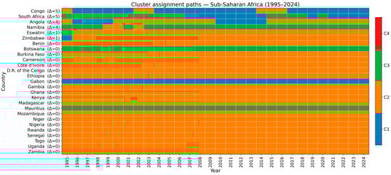
Figure 13. Country archetype evolution for Sub-Saharan Africa (Δ = cluster transition counts).

A moderated pattern of club convergence is observed at the regional level. Western Europe and North America remain at the frontier, while sustained advancement is observed in Eastern Europe. East and Central Asia combines frontier stability with incremental catch up, whereas ASEAN shows gradual progress through the C2 to C3 corridor alongside a persistent lower tail. Sub-Saharan Africa remains largely stationary, and MENA clusters around an intermediate level with limited advancement. Latin America is characterized by stable C2 and C3 clubs with boundary movement and episodic upgrading in a subset of cases. Permanence is most evident in Western Europe and North America through stable C4 membership and in Sub-Saharan Africa through long C2 spells. By contrast, oscillation and boundary churn are concentrated in Latin America and the Caribbean and in selected transitional cases in ASEAN and East and Central Asia. Reversals are localized and typically appear as short dips around the C2-to-C3 or C3-to-C4 boundaries (Table 3). These regional patterns reinforce RQ3 by confirming persistent clubs with selective mobility and varied adjustment speeds (Eleftheriou et al., 2024; Renou-Maissant et al., 2022). They are also consistent with RQ2, given declining dispersion and smaller frontier gains that align with partial decoupling.

Table 3. Region-level summary of dominant archetypes and mobility patterns across 1995–2024.

Region	Dominant Archetype	Typical Mobility Pathways	Oscillation or Reversal Tendency	Permanence Tendency
ASEAN	C2–C3 mix with C3 rising (plus persistent C1 and a C4 anchor)	C2 → C3 and C1 → C3	Low	Medium
East and Central Asia	Bifurcated profile (C4 anchors + C1 persistence + C3 middle)	C2 → C3 (Armenia) and C3 → C4 (Korea); localized C3 → C1 dips (China)	Low	High
South Asia	C2 dominant with selective C3 upgrading	C2 → C3 (India, Sri Lanka)	Very low	High
Oceania	C4 Dominant	Stable C3 and C4	Very low	Very High
Europe West	C4 dominant	Mostly stable C4;	Very low	Very high
Europe East	C3 with sustained upgrading into C4 plus a persistent C1 cases	Limited: C3 → C4	Low	High
North America	C4 anchored with a stable C3 member	No mobility observed	Very low	Very high
Latin America and Caribbean	C2 and C3 dominant	C2 → C3 and C3 → C4	Medium	Medium
Middle East and North Africa	C1 and C3 dominant	C1 → C3 and C3 → C4 (limited)	Low	Medium
Sub-Saharan Africa	C2 dominant with sparse C3 and localized C1 outliers	Mostly stable C2; rare C2 → C3 upgrades	low	High

5.5. Frontier Slowdown in the Environmental Capability Space

The distance DDI profile (Figure 14) shows clear distance-conditioned catch-up. Average DDI is near zero at small gaps and turns positive at larger distance, indicating that countries farther from the ideal reduce distance faster. Negative DDI values indicate divergence from the reference ideal point, meaning that when countries are already close to the ideal reference point they can be pushed away from it. This pattern strengthens RQ2 by tying fairness to a frontier slowdown. It also shows that the ideal state is dynamically unstable. Systems can approach it, but gains compress near the ideal as diffusion advantages fade and diminishing returns set in (Markard et al., 2012). Cluster overlays reveal systematic heterogeneity, which strengthens RQ3. C1 improves only when distance is large. This implies that operational refinements alone do not close distance without parallel expansion of capacity. C2 shows small but steady gains with distance, consistent with incremental adoption. C3 exhibits the strongest catch-up at large distance, suggesting enabling baselines for fast copying. C4 improves strongly at larger distances, but the gains diminish quickly as distance to the ideal narrows near the frontier. This pattern is consistent with deep decarbonization and the need for rapid absolute reductions, which can slow net advance (Haberl et al., 2020; Renou-Maissant et al., 2022).

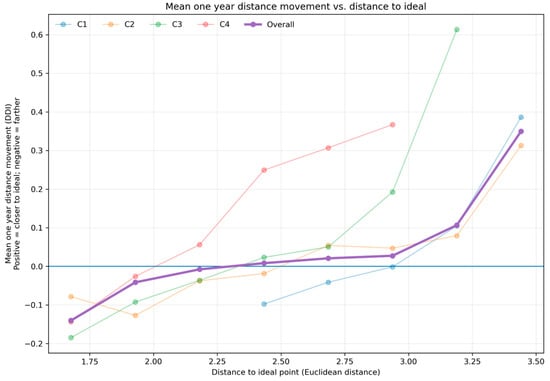
Figure 14. Mean one year improvement in vs. distance to ideal by cluster. Positive DDI indicates average movement toward ideal reference point at that initial distance, while negative DDI indicates average movement away from it.

Effectiveness (DDI per step) rises with distance to the ideal and turns negative close to the frontier (Figure 15). When distance is large, movement tends to translate into larger net distance reductions, whereas as distance narrows the gains plateau and can become negative, indicating divergence from the reference ideal point near the frontier. Greater effort converts into smaller net proximity gains as portfolios approach high capability. This helps explain tempered club convergence. Robust within-club tightening is observed alongside persistent cross-club heterogeneity, even as overall opportunity remains broadly similar (Erdogan & Okumus, 2021; Gilli et al., 2013; Amann et al., 2013).

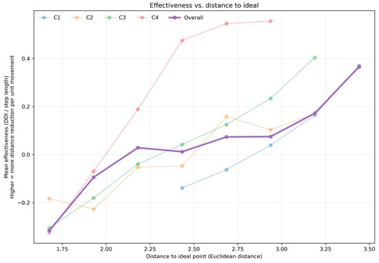
Figure 15. Mean movement effectiveness vs. distance to ideal point by cluster. Effectiveness is measured as DDI per step length.

5.6. Robustness and Sensitivity Checks

Uncertainty in indicator construction, scaling, and relative emphasis across lenses was evaluated using sensitivity perturbations. In this way, plausible changes arising from indicator refinement or alternative operationalizations were approximated without redefining the full framework. Cluster assignment stability was assessed using ARI between the baseline pooled partition and partitions re estimated under one at a time lens reweighting within a ±20% band (0.8–1.2) (Figure 16). Across this plausible range, the clustering remains highly stable, with ARI generally close to unity. PC and RDP are particularly robust. DM shows the largest decline when upweighted. This pattern indicates that emphasizing the momentum dimension reorients the clustering geometry more strongly, even under moderate perturbation. Changes in membership are concentrated at the lower boundary. Marginal observations primarily shift between C1 and C2, while the upper archetype C4 remains highly stable. The full robustness figures are reported in Appendix A (Figure A1 and Figure A2).

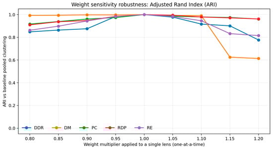
Figure 16. ARI between baseline pooled clustering and partitions re-estimated under one at a time lens reweighting (0.8–1.2).

Sensitivity to the CO₂ threshold was evaluated by varying the RDP limit by ±20% around the baseline (1.9 t CO₂ per capita) (Figure 17). The distribution shifts left under higher limits, as more country–year observations fall below the tightened sustainability ceiling, yet the overall shape and dispersion remain largely preserved. The clustering remains stable, with ARI values close to unity across the perturbation range, confirming that the four-archetype structure is insensitive to moderate changes in the carbon boundary. Minor reassignments occur mainly between mid-range groups, as shown in Appendix A (Figure A3), while the top archetype remains virtually unchanged.

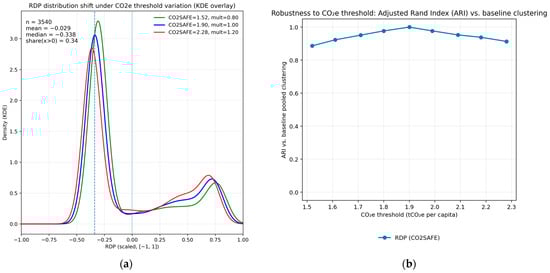
Figure 17. CO₂ threshold sensitivity: (a) distributional shift of RDP lens under varying tCO₂e per capita threshold limits. The vertical blue dashed line indicates the base case median RDP score (threshold = 1.90 tCO₂e per capita), and (b) ARI robustness of pooled clustering.

6. Conclusions and Policy Implication

The evidence shows a stable environmental capability landscape with four enduring archetypes and decreasing cross-sectional inequality from 1995 to 2024. Clear separation exists in the PCA plane. Persistent cluster membership is observed, and centroid path crossing is minimal. Regionally, high capability frontier archetypes are concentrated in Western Europe and North America, together with Japan, the Republic of Korea, and a few city-state economies. Low inequality in attainment, measured by the Gini and Palma indices, suggests similar opportunities to approach the ideal for majority of the countries. Outcomes in this study are determined by how countries navigate the capability space rather than by income alone. Mobility is selective and path-dependent. Transition matrices are diagonal dominated, and gradual permanent upgrades are observed, as seen in the steady advancement of several Eastern European and ASEAN economies. These findings align with tempered club convergence driven by cumulative capability, diffusion, and coordination costs.

Building on the findings, policy implications can be framed by a country’s position in capability space and its associated archetype. For C1, moderate productive capacity coexists with low efficiency, high depletion, and limited remaining headroom. In this period, this cluster includes several resource-exporting economies in the Middle East and North Africa. Priorities include restructuring and upgrading existing capacity with proven low-carbon and efficiency-improving technologies, reducing depletion burdens, and strengthening coordination mechanisms. For C2, capability is low but depletion pressure is relatively low and remaining development potential is high. This cluster is common in South Asia, much of Sub-Saharan Africa, and lower-income ASEAN member. Policy should focus on scaling proven technologies, reinforcing regulations, expanding concessional finance, and building implementation capacity. For C3, balanced intermediate profiles characterize many higher-income ASEAN and Latin American, and middle-income European economies. Returns are obtained from systems integration and diffusion, including grid flexibility and cross-sector coordination, so that spatial challenges are transformed into benefits. For C4, countries are located at the high capability frontier but remaining headroom is limited. This cluster is found mainly in Western Europe, North America, Japan, and a few city-state economies. Emphasis shifts to innovation that relaxes environmental constraints, demand management, and deeper decarbonization with cross-sector coordination.

Instruments for sustainable transition should be allocated accordingly. Nations far from the ideal can achieve substantial reductions through established practices and targeted investments. Policy should prioritize technology transfer, standards, and concessional financing. In regions near the frontier, where incremental effectiveness diminishes, focus should shift to coordination, reform, and incentives that improve effectiveness. Support should emphasize permanence. Programs should target upgrades lasting at least five years and protect against boundary reversals. Regional cooperation that reduces diffusion costs can expedite progress. These distance-aware and archetype-specific strategies offer a pathway to advancement in a world of persistent capabilities and moderated convergence.

Despite these findings, several limitations suggest avenues for future research. First, the analysis is restricted to 1995 to 2024, so earlier episodes of large-scale energy and environmental disruption are not observed. If the sample is extended backward, the durability of the archetypes could be assessed over longer cycles. Second, the lens set can be expanded. In particular, remaining development potential is operationalized using a CO₂ based constraint, whereas a more comprehensive representation aligned with planetary boundaries would be desirable. This extension could incorporate additional pressures such as land and forest change and water use. However, consistent long-run cross-country coverage for these indicators remains limited in large samples, so multi boundary constraints are left for future work. Third, the results characterize pathways and archetypes but do not identify the underlying social and institutional processes that shape divergence among countries with similar starting positions. While PC and DM proxy some internal capabilities, deeper qualitative and country specific work would be needed to explain why particular routes are taken.

References

- Agusdinata, D. B., Aggarwal, R., & Ding, X. (2020). Economic growth, inequality, and environment nexus: Using data mining techniques to unravel archetypes of development trajectories. Environment, Development and Sustainability, 23, 6234–6258. [Google Scholar] [CrossRef]
- Alotaiq, A. (2024). Global low carbon transitions in the power sector: A machine learning clustering approach using archetypes. Journal of Economy and Technology, 2, 95–127. [Google Scholar] [CrossRef]
- Amann, M., Klimont, Z., & Wagner, F. (2013). Regional and global emissions of air pollutants: Recent trends and future scenarios. Annual Review of Environment and Resources, 38, 31–55. [Google Scholar] [CrossRef]
- Arogundade, S., Hassan, A., Akpa, E., & Biyase, M. (2023). Closer together or farther apart: Are there club convergence in ecological footprint? Environmental Science and Pollution Research, 30, 15293–15310. [Google Scholar] [CrossRef]
- Basu, S., Ogawa, T., & Ishihara, K. N. (2022). The methods and factors of decoupling energy usage and economic growth. In Waste-to-energy approaches towards zero waste (pp. 269–313). Elsevier. [Google Scholar] [CrossRef]
- Berndt, E. R., & Wood, D. O. (1975). Technology, prices, and the derived demand for energy. Review of Economics and Statistics, 57, 259–268. [Google Scholar] [CrossRef]
- Bluszcz, A. (2016). A comparative analysis of selected synthetic indicators of sustainability. Procedia Social and Behavioral Sciences, 220, 40–50. [Google Scholar] [CrossRef]
- Chancel, L. (2022). Global carbon inequality over 1990–2019. Nature Sustainability, 5, 931–938. [Google Scholar] [CrossRef]
- Chu, L. K., & Hoang, D. P. (2022). The shadow economy–environmental quality nexus in OECD countries: Empirical evidence from panel quantile regression. Environmental Science and Pollution Research, 29, 65233–65258. [Google Scholar] [CrossRef] [PubMed]
- Dosi, G., & Nelson, R. R. (2010). Technical change and industrial dynamics as evolutionary processes. In B. H. Hall, & N. Rosenberg (Eds.), Handbook of the economics of innovation (Vol. 1, pp. 51–127). Elsevier. [Google Scholar] [CrossRef]
- Eisenack, K., Villamayor-Tomas, S., Epstein, G., Kimmich, C., Magliocca, N., Manuel-Navarrete, D., Oberlack, C., Roggero, M., & Sietz, D. (2019). Design and quality criteria for archetype analysis. Ecology and Society, 24(3), 6. [Google Scholar] [CrossRef]
- Ekins, P. (1993). “Limits to growth” and “sustainable development”: Grappling with ecological realities. Ecological Economics, 8, 269–288. [Google Scholar] [CrossRef]
- Eleftheriou, K., Nijkamp, P., & Polemis, M. L. (2024). Club convergence of sustainable development: Fresh evidence from developing and developed countries. Economic Change and Restructuring, 57, 32. [Google Scholar] [CrossRef]
- Emir, F., Balcilar, M., & Shahbaz, M. (2019). Inequality in carbon intensity in EU-28: Analysis based on club convergence. Environmental Science and Pollution Research, 26, 3308–3319. [Google Scholar] [CrossRef] [PubMed]
- Erdogan, S., & Okumus, I. (2021). Stochastic and club convergence of ecological footprint: An empirical analysis for different income group of countries. Ecological Indicators, 121, 107123. [Google Scholar] [CrossRef]
- Esty, D. C., Levy, M., Srebotnjak, T., & de Sherbinin, A. (2005). Environmental sustainability index: Benchmarking national environmental stewardship. Yale Center for Environmental Law and Policy. [Google Scholar]
- Everitt, B. S., Landau, S., Leese, M., & Stahl, D. (2011). Cluster analysis (5th ed.). John Wiley & Sons, Ltd. [Google Scholar] [CrossRef]
- Feenstra, R. C., Inklaar, R., & Timmer, M. P. (2015). The next generation of the Penn World Table. American Economic Review, 105, 3150–3182. [Google Scholar] [CrossRef]
- Gilli, M., Mazzanti, M., & Nicolli, F. (2013). Sustainability and competitiveness in evolutionary perspectives: Environmental innovations, structural change and economic dynamics in the EU. The Journal of Socio-Economics, 45, 204–215. [Google Scholar] [CrossRef]
- Gini, C. (1912). Variabilità e mutabilità: Contributo allo studio delle distribuzioni e delle relazioni statistiche. Tipografia di Paolo Cuppini. [Google Scholar]
- Gómez, M., & Rodríguez, J. C. (2024). Analysis of the convergence of environmental sustainability and its main determinants: The case of the Americas (1990–2022). Sustainability, 16, 6819. [Google Scholar] [CrossRef]
- Haberl, H., Wiedenhofer, D., Virág, D., Kalt, G., Plank, B., Brockway, P., & Creutzig, F. (2020). A systematic review of the evidence on decoupling of GDP, resource use and GHG emissions. Environmental Research Letters, 15, 063002. [Google Scholar] [CrossRef]
- Haider, S., & Akram, V. (2019). Club convergence analysis of ecological and carbon footprint: Evidence from a cross-country analysis. Carbon Management, 10, 451–463. [Google Scholar] [CrossRef]
- Halvorsen, R., & Smith, T. R. (1984). On measuring natural resource scarcity. Journal of Political Economy, 92(5), 954–964. [Google Scholar] [CrossRef]
- Hansen, U. E., Nygaard, I., Romijn, H., Wieczorek, A., Kamp, L. M., & Klerkx, L. (2018). Sustainability transitions in developing countries: Stocktaking, new contributions and a research agenda. Environmental Science & Policy, 84, 198–203. [Google Scholar] [CrossRef]
- Haque, M. S. (2000). Environmental discourse and sustainable development: Linkages and limitations. Ethics and the Environment, 5, 3–21. [Google Scholar] [CrossRef]
- Hsu, A., Esty, D. C., Levy, M. A., & de Sherbinin, A. (2016). 2016 Environmental performance index. Yale Center for Environmental Law and Policy. [Google Scholar]
- Intergovernmental Panel on Climate Change (IPCC). (2022). Global warming of 1.5 °C: IPCC special report on impacts of global warming of 1.5 °C above pre-industrial levels in context of strengthening response to climate change, sustainable development, and efforts to eradicate poverty. Cambridge University Press. [Google Scholar]
- Jackson, T. (2009). Prosperity without growth: Economics for a finite planet. Earthscan. [Google Scholar]
- Kaufman, L., & Rousseeuw, P. J. (1990). Finding groups in data: An introduction to cluster analysis. Wiley. [Google Scholar]
- Kaya, Y. (1990). Impact of carbon dioxide emission control on GNP growth: Interpretation of proposed scenarios. IPCC Energy and Industry Subgroup, Response Strategies Working Group. [Google Scholar]
- Krautkraemer, J. A. (1998). Nonrenewable resource scarcity. Journal of Economic Literature, 36, 2065–2107. [Google Scholar]
- Küppers, M., Metzger, M., Huber, M., & Paulus, S. (2019, June 23–27). Archetypes of country energy systems. 2019 IEEE Milan PowerTech (PowerTech) (pp. 1–6), Milan, Italy. [Google Scholar]
- Ma, F., Wang, H., Tzachor, A., Hidalgo, C. A., Schandl, H., Zhang, Y., Zhang, J., Chen, W.-Q., Zhao, Y., Zhu, Y.-G., & Fu, B. (2025). The disparities and development trajectories of nations in achieving the sustainable development goals. Nature Communications, 16, 1107. [Google Scholar] [CrossRef] [PubMed]
- MacQueen, J. (1967). Some methods for classification and analysis of multivariate observations. In Proceedings of the fifth Berkeley symposium on mathematical statistics and probability, Berkeley, CA, USA, 21 June–18 July 1965 and 27 December 1965–7 January 1966 (Vol. 1, pp. 281–297). University of California Press. [Google Scholar]
- Markard, J., Raven, R., & Truffer, B. (2012). Sustainability transitions: An emerging field of research and its prospects. Research Policy, 41, 955–967. [Google Scholar] [CrossRef]
- Moallemi, E. A., Hosseini, S. H., Eker, S., Gao, L., Bertone, E., Szetey, K., & Bryan, B. A. (2022). Eight archetypes of SDG synergies and trade-offs. Earth’s Future, 10, e2021EF002621. [Google Scholar] [CrossRef]
- OECD. (2002). Indicators to measure decoupling of environmental pressure from economic growth. OECD Publishing. [Google Scholar]
- OECD. (2011). Towards green growth. OECD Publishing. [Google Scholar]
- Osorio, L. A. R., Lobato, M. O., & del Castillo, X. Á. (2005). Debates on sustainable development: Towards a holistic view of reality. Environment, Development and Sustainability, 7, 501–518. [Google Scholar] [CrossRef]
- Palma, J. G. (2011). Homogeneous middles vs. heterogeneous tails, and the end of the “inverted U”: It is all about the share of the rich. Development and Change, 42(1), 87–153. [Google Scholar] [CrossRef]
- Panopoulou, E., & Pantelidis, T. (2009). Club convergence in carbon dioxide emissions. Environmental and Resource Economics, 44, 47–70. [Google Scholar] [CrossRef]
- Partelow, S., Nagel, B., Gentry, R., Gephart, J., & Rocha, J. (2025). Archetypes of aquaculture development across 150 countries. Aquaculture, 595, 741484. [Google Scholar] [CrossRef]
- Pedde, S., Kok, K., Hölscher, K., Oberlack, C., Harrison, P. A., & Leemans, R. (2019). Archetyping shared socioeconomic pathways across scales: An application to central Asia and European case studies. Ecology and Society, 24(4), 30. [Google Scholar] [CrossRef]
- Peters, G. P., Minx, J. C., Weber, C. L., & Edenhofer, O. (2011). Growth in emission transfers via international trade from 1990 to 2008. Proceedings of the National Academy of Sciences, 108, 8903–8908. [Google Scholar] [CrossRef] [PubMed]
- Redclift, M. (2005). Sustainable development (1987–2005): An oxymoron comes of age. Sustainable Development, 13, 212–227. [Google Scholar] [CrossRef]
- Renou-Maissant, P., Abdesselam, R., & Bonnet, J. (2022). Trajectories for energy transition in EU-28 countries over the period 2000–2019: A multidimensional approach. Environmental Modeling & Assessment, 27, 525–551. [Google Scholar] [CrossRef]
- Rockström, J., Steffen, W., Noone, K., Persson, Å., Chapin, F. S., Lambin, E., & Foley, J. A. (2009). A safe operating space for humanity. Nature, 461, 472–475. [Google Scholar] [CrossRef] [PubMed]
- Romer, P. M. (1990). Endogenous technological change. Journal of Political Economy, 98, S71–S102. [Google Scholar] [CrossRef]
- Ruggerio, C. A. (2021). Sustainability and sustainable development: A review of principles and definitions. Science of the Total Environment, 786, 147481. [Google Scholar] [CrossRef]
- Sen, A. (1999). Development as freedom. Oxford University Press. [Google Scholar]
- Siche, R., Agostinho, F., Ortega, E., & Romeiro, A. (2008). Sustainability of nations by indices: Comparative study between environmental sustainability index, ecological footprint and the emergy performance indices. Ecological Economics, 66, 628–637. [Google Scholar] [CrossRef]
- Sietz, D., Frey, U., Roggero, M., Gong, Y., Magliocca, N. R., Rong, T., Janssen, P., & Václavík, T. (2019). Archetype analysis in sustainability research: Methods and applications. Ecology and Society, 24(3), 34. [Google Scholar] [CrossRef]
- Sneddon, C., Howarth, R. B., & Norgaard, R. B. (2006). Sustainable development in a post-Brundtland world. Ecological Economics, 57, 253–268. [Google Scholar] [CrossRef]
- Solow, R. M. (1956). A contribution to the theory of economic growth. Quarterly Journal of Economics, 70, 65–94. [Google Scholar] [CrossRef]
- Stefani, G., Biggeri, M., & Ferrone, L. (2022). Sustainable transitions narratives: An analysis of the literature through topic modelling. Sustainability, 14, 2085. [Google Scholar] [CrossRef]
- Steffen, W., Richardson, K., Rockström, J., Cornell, S. E., Fetzer, I., Bennett, E. M., & Sörlin, S. (2015). Planetary boundaries: Guiding human development on a changing planet. Science, 347, 1259855. [Google Scholar] [CrossRef] [PubMed]
- Stern, D. I., Common, M. S., & Barbier, E. B. (1996). Economic growth and environmental degradation: The environmental Kuznets curve and sustainable development. World Development, 24(7), 1151–1160. [Google Scholar] [CrossRef]
- Terluin, I. J. (2003). Differences in economic development in rural regions of advanced countries: An overview and critical analysis of theories. Journal of Rural Studies, 19, 327–344. [Google Scholar] [CrossRef]
- Ulucak, R., & Apergis, N. (2018). Does convergence really matter for the environment? An application based on club convergence and on the ecological footprint concept for the EU countries. Environmental Science and Policy, 80, 21–27. [Google Scholar] [CrossRef]
- Wackernagel, M., & Rees, W. (1996). Our ecological footprint: Reducing human impact on the earth. New Society Publisher. [Google Scholar]
- World Bank. (2025). World development indicators. Data set, world bank databank. Available online: https://databank.worldbank.org/data/download/WDI_EXCEL.zip (accessed on 30 July 2025).
- World Commission on Environment and Development (WCED). (1987). Our common future. Oxford University Press. [Google Scholar]
Disclaimer/Publisher’s Note: The statements, opinions and data contained in all publications are solely those of the individual author(s) and contributor(s) and not of MDPI and/or the editor(s). MDPI and/or the editor(s) disclaim responsibility for any injury to people or property resulting from any ideas, methods, instructions or products referred to in the content. |
© 2026 by the authors. Licensee MDPI, Basel, Switzerland. This article is an open access article distributed under the terms and conditions of the Creative Commons Attribution (CC BY) license.