One Model Fits All? Evaluating Bankruptcy Prediction Across Different Economic Periods

Abstract

Financial distress prediction models are widely used to support risk management. However, economic turbulence, such as the COVID-19 pandemic, can disrupt the relationships between financial indicators and distress, thus threatening the stability and accuracy of the models’ predictions. In this study, the stability of bankruptcy prediction models is examined on a large sample of small and medium-sized enterprises (SMEs) in Slovakia. Three periods are distinguished: the pre-pandemic years 2018–2019, the COVID-19 pandemic years 2020–2021, and the post-pandemic recovery years 2022–2023. Two approaches to model construction are compared: separate models are estimated for each period, and a single comprehensive model covering all three periods is constructed with a period-specific indicator among the predictors. Publicly available financial data and machine learning methods are employed, and model performance is evaluated using common classification metrics. Differences in performance are revealed, indicating whether period-specific models provide superior predictive accuracy or whether a universal model can adapt to changing economic conditions. The robustness, stability, predictive power, and practical applicability of both approaches are assessed, and the influence of economic fluctuations on accuracy is demonstrated. The findings provide guidance on selecting modelling strategies across different economic environments and offer recommendations for further developing and implementing predictive models in volatile financial conditions.

1. Introduction

Predictive models are essential in business practice, as they enable early risk identification and support effective decision-making. Their use is particularly critical in financial distress prediction, where they can help minimise financial losses for all stakeholders (Hammond et al., 2023). Assessing the financial sustainability of business partners, customers, or financial institutions is particularly important given that corporate failures result in substantial economic losses not only for shareholders and creditors but also for society, imposing broader social and economic costs (Zelenkov & Volodarskiy, 2021; Laitinen et al., 2023). However, financial distress or bankruptcy can often be anticipated through various warning signals. Early recognition and accurate interpretation of these signals enable managers to take timely and effective actions to mitigate the consequences of a potential crisis (Balina et al., 2021). Consequently, the ability to reliably predict corporate failure has become a vital element of strategic decision-making in both financial and non-financial firms (Citterio, 2024).

Currently, the business environment faces challenges such as global health crises, supply chain disruptions, geopolitical tensions, and rising inflation and interest rates, all of which fundamentally affect firms’ financial stability (Svabova et al., 2022). The COVID-19 pandemic has made even large companies vulnerable, emphasising the need for reliable tools to identify risks and predict potential insolvency (Archanskaia et al., 2023). Therefore, the reliability and robustness of prediction models are particularly important not only for the affected companies but also for investors, creditors, and regulators, who must make informed decisions under conditions of uncertainty (Chakrabarti et al., 2024).

Conventional bankruptcy prediction models, including Altman’s Z-score and logit models, have typically been developed and tested under economically stable conditions (Shi & Li, 2024; Bobitan & Dumitrescu, 2024). However, their application during times of crisis may yield misleading results due to the dynamic evolution of the relationship between financial ratios and the probability of bankruptcy over time (Dasilas & Rigani, 2024). Therefore, it is crucial to assess their effectiveness at different stages of the economic cycle (Papik & Papikova, 2024). Despite the growing importance of this issue, the literature contains relatively limited research that methodologically compares the performance of predictive models across different economic conditions. This research area offers the potential for deeper analysis that can contribute to more effective financial risk management and the development of more robust predictive tools applicable in practice.

Although this study focuses primarily on classification-based predictive techniques, it is important to recognise that time-series forecasting methods have also played a major role in economic and financial prediction. The Box-Jenkins ARIMA framework has historically been one of the earliest and most influential approaches for modelling in economics (Box & Jenkins, 1970; Box et al., 2016). Its relevance extends across the economic and social sciences, where ARIMA models have been widely applied to predict macroeconomic aggregates, market movements, and firm-level financial ratios (Chatfield, 2003; Hyndman & Athanasopoulos, 2018). In financial distress research, time-series approaches can complement ratio-based classification models by modelling the temporal evolution of financial indicators or macroeconomic conditions that shape insolvency risk (Kaczmarek, 2012). The usefulness of ARIMA has been reinforced during periods of heightened volatility, including the COVID-19 pandemic, when it was widely used to generate reliable forecasts. For instance, Das (2020) demonstrated the strong predictive performance of the ARIMA model in forecasting COVID-19 incidences across highly affected countries, highlighting the method’s robustness and accuracy. While our study does not employ ARIMA directly, acknowledging this methodological stream extends the broader forecasting context within which bankruptcy prediction research is situated.

Therefore, the impact of different economic periods on the accuracy of financial distress prediction is analysed in this paper. Moreover, two approaches to model creation are compared. First, separate models for three different economic periods (pre-pandemic, pandemic, and post-pandemic) are developed. The period 2022–2023 is referred to as the post-pandemic period, representing the phase after pandemic-related restrictions ended. We acknowledge that this period includes additional shocks, most notably the war in Ukraine and subsequent inflationary pressures. Therefore, this period is not treated as fully homogeneous but rather as a distinct phase characterised by macroeconomic conditions different from those of the acute pandemic years. Second, a single comprehensive model is created that incorporates period-indicating variables. The research examines whether models customised for specific business cycle phases exhibit greater predictive capability than a universal model with the period indicator.

The motivation for this study arises from the growing need to understand how economic disruptions, particularly extreme events such as the COVID-19 pandemic, affect the stability and reliability of financial distress prediction models. Although bankruptcy prediction has been extensively studied for decades, the existing literature rarely examines whether these models’ performance remains consistent when economic conditions change significantly. Most prior studies focus either on crisis or on stable periods alone, without systematically comparing predictive accuracy across multiple phases of the economic cycle or assessing whether a unified modelling framework can adapt to shifting financial dynamics. This research gap is particularly important because, during the pandemic, companies faced abrupt financial pressures, structural changes in cash flows, and increased liquidity risk, raising concerns about whether prediction models developed under normal conditions remain stable in periods of economic instability. For risk managers, investors, regulators, and policymakers, the ability to rely on prediction models during turbulent periods is essential for timely intervention, credit allocation, and systemic risk monitoring. By addressing this gap, this study responds to these needs by providing a systematic comparison of model performance across three distinct economic periods and evaluating whether a single comprehensive model can maintain predictive accuracy even when the economic environment changes significantly.

Reflecting the aim of the research, the following question and hypotheses were set for the purpose of this research:

RQ: How does changing the modelling approach affect the ability to predict financial distress over different economic periods?

H1. 

The relative predictive performance ranking of modelling techniques differs significantly across economic periods (pre-pandemic, pandemic, and post-pandemic periods).

H2. 

Period-specific models achieve higher accuracy than a universal model with a period indicator.

The next parts of the paper are organised as follows. The Literature review section highlights the current state of financial distress prediction. Section 2 explains the study methodology, briefly characterises the modelling techniques, and describes the data used in the study. Section 3 presents the results for both modelling approaches. The final section concludes the study.

Literature Review

The prediction of corporate failure has been extensively studied since the work of Beaver (1966) and Altman (1968). Among the best-known models is Altman’s Z-score, based on multivariate discriminant analysis (Khashei et al., 2024), which is widely used due to its ease of application and relative reliability (Alam et al., 2021). However, its limitations have also been highlighted in the literature, including its origins in US industrial firms, the use of static indicators, and its sensitivity to accounting manipulations (Dieperink et al., 2024).

The predictive model’s performance is strongly influenced by economic conditions. Using a random forest algorithm, the key factors contributing to the increased bankruptcy risk during the COVID-19 pandemic were identified by Bozkurt and Kaya (2023), highlighting that the country’s macroeconomic conditions had an even greater impact on bankruptcy risk. These results were confirmed by Durana et al. (2025a) for the V4 countries, emphasising the importance of national economic specificities, and by Narvekar and Guha (2021), who highlighted the significance of business cycle phases for model performance.

The importance of considering the broader context of corporate bankruptcies is also emphasised by Kitowski et al. (2022) and Amankwah-Amoah et al. (2021). It is argued that the focus should be on globalisation, accelerating change, and new forms of risk that reduce the effectiveness of existing prediction models. It is also pointed out that relying on experience can become a disadvantage precisely because of the strategic rigidity of firms.

Similarly, it was found by Papik and Papikova (2022) that models trained on pre-pandemic data are significantly less reliable during a pandemic. During the crisis, debt indicators were important, while liquidity dominated the stable period. Similar findings are reported in the study by Spiler et al. (2022), in which traditional models failed to account for structural changes during the 2020 pandemic crisis, resulting in a decline in prediction accuracy. Therefore, the development of more flexible models that can respond to market dynamics in times of crisis is recommended.

Modifications to the model for the crisis period are also discussed by Halteh (2025), whose research found that the COVID-19 crisis primarily affected larger firms. A divergence in factors affecting financial distress between small and large firms was also revealed, underscoring the need for firm-specific models. While small firms were mainly affected by liquidity and debt, large firms were primarily impacted by profitability and capital structure.

The methodology for model creation was discussed by Shetty et al. (2022), and the reliability of simple financial data models was demonstrated. However, the benefits of machine learning techniques are highlighted by Mate et al. (2023) and Durica et al. (2023). In the study of Elsayed et al. (2024), the random forest algorithm achieved the best results. Moreover, it was emphasised that the correct selection of input variables significantly enhances prediction accuracy.

2. Methodology

In this study, several models for predicting companies’ financial distress have been developed using two modelling approaches. Firstly, separate period-specific models for the pre-pandemic, pandemic, and post-pandemic periods were developed. Secondly, a comprehensive model covering all periods that contains the period-indicating variables among the potential predictors was created. Several techniques for model development were selected, including CART, CHAID, and C5 decision trees, as well as logistic regression, discriminant analysis, and neural networks. All these methods are suitable for the classification task of predicting the company’s financial state. Therefore, in the following section, all methods of model creation and the measures for their evaluation are briefly characterised.

2.1. Modelling Techniques Used in the Study

Decision tree algorithms are widely used in predictive modelling, mainly due to their interpretability and flexibility. These algorithms recursively partition the dataset into increasingly homogeneous subsets based on the decision rules derived from the explanatory variables (Rudd Mph & Priestley, 2017). In decision-tree terminology, the root node represents the initial node containing the entire dataset before any partitioning occurs. From this point, the algorithm applies splitting rules based on selected predictor variables to divide the data into more homogeneous groups. The splitting variables and the splitting criteria are selected automatically according to the criterion of best separation between or among the groups of the outcome variable. This criterion varies across decision tree techniques. The nodes resulting from these intermediate splits are called internal nodes; each contains a subset of observations and may be further partitioned if doing so improves node purity. The process continues until no additional meaningful splits can be made or a stopping criterion is reached. The splitting process stops when the stop criteria are met, such as a maximum tree depth, a minimum number of cases in a parent or child node, or a minimal change in impurity. At this stage, the algorithm produces terminal nodes, also known as leaves, which represent the final, indivisible subsets of the data. The entire process yields a tree-structured model, where each internal node represents a division based on a predictor variable, and each leaf node represents a specific prediction. In classification tasks, the predicted class is determined by the modal class; in regression tasks, by the average value. The tree should be rewritten into a set of if-then criteria or depicted as a tree. This hierarchical representation enables decision trees to capture non-linear relationships and interaction effects without requiring distributional assumptions or prior specification of functional forms. The tree prediction model should be used for both predictive and descriptive purposes, as it can not only classify new cases but also provide easily interpretable relationships between the predictors and the outcome.

The CART (Classification and Regression Trees) algorithm, originally introduced by Breiman et al. (1984), represents one of the most influential methods in the family of decision tree techniques. It is a non-parametric predictive modelling method based on recursive partitioning of the predictor space. CART constructs a decision tree by recursively partitioning the data into increasingly homogeneous subsets according to values of the explanatory variables. The tree is binary, meaning each parent node has two child nodes. At each step, the method evaluates potential splits and selects the one automatically that yields the greatest improvement in node purity. The input variables for these splits are chosen automatically based on a criterion that maximises the homogeneity of the resulting subsets. For classification tasks, the most frequently used criterion for measuring the homogeneity is the Gini impurity index, while regression trees rely on minimising the variance within nodes (Loh, 2011). In our study, the technique is employed to solve the classification task, with a minimum impurity change of 0.0001. The stopping rules are as follows: a maximum tree depth of 5, a minimum of 2% of records in the parent branch, and 1% of records in the child branch. To address the problem of overfitting, in which the resulting CART model becomes overly complex, the tree can be pruned by removing branches that do not significantly improve the model’s prediction accuracy (Gabrikova et al., 2023).

CHAID (Chi-Square Automatic Interaction Detection) is a decision tree algorithm that utilises chi-square statistical tests to identify the optimal splits at each step of the recursive partitioning process. For continuous predictors, CHAID groups values into categories prior to testing, whereas for categorical predictors, it merges categories that do not differ significantly from each other with respect to the outcome variable. This merging ensures that only the categories with distinct relationships with the outcome remain (Kass, 1980; Song & Lu, 2015). CHAID trees can have multiple branches at each node, making them more universal and capable of capturing more complex relationships and interactions among the predictors and the outcome (Magidson, 1993). However, as CHAID employs statistical significance testing, the computational complexity in the case of large datasets is likely to be overly high (Durica et al., 2019; Kicova et al., 2025). The stopping criteria used in this study are as follows: a maximum tree depth of 5, a minimum of 2% of records in the parent branch, and 1% of records in the child branch, a significance level for splitting and merging the continuous predictors of 0.05, and a minimum change in expected cell frequencies for categorical predictors (if any) of 0.001.

The C5.0 algorithm constructs decision trees by selecting predictors and their splitting criteria based on the concept of information entropy. Each parent node can be divided into multiple child nodes, allowing for the capture of the complexity of the relationships among the variables. This technique is particularly known for its speed, accuracy, and ability to handle noisy data (M.-Y. Chen, 2011). The stopping criteria used in this study are defined by a pruning severity of 75% and a minimum of 2 records in the child branch. This technique enables pruning after tree growth, where branches without a significant contribution to the model’s predictive performance are omitted to improve readability and simplify the tree structure (Massahi Khoraskani et al., 2018; Vlaović Begović & Bonić, 2020).

Logistic regression (LR) is a widely used statistical technique for modelling the probability of a binary outcome and has long been applied to financial distress prediction, primarily due to its simplicity and interpretability. It estimates the probability of a data case belonging to a particular class of the outcome variable, which is most commonly binomial, by modelling the log-odds as a linear combination of the explanatory variables (Hosmer et al., 2013). In our study, the LR models the probability of a company’s financial distress, given the values of the financial ratios and other variables included in the model. Because the outcome of interest in LR is a probability, it must, by definition, lie between 0 and 1. Therefore, a probability model must ensure that no combination of predictor variables produces values outside this range. A simple linear regression model, expressed as a linear combination of predictors, cannot guarantee this restriction, because the linear predictor can take any real value. Consequently, the estimated probabilities could fall below 0 or above 1, which is mathematically invalid and meaningless for classification. To avoid this problem, logistic regression applies a link function that transforms the real values into the $\left(0,1\right)$ interval. Such a transformation is achieved by modelling the log-odds (or logit) of the outcome rather than the probability itself. Formally, if $p$ denotes the probability of financial distress, the logistic model specifies that

$$\log {\displaystyle \frac{p}{1-p}}={\beta }_0+{\beta }_1{x}_1+\cdots +{\beta }_k{x}_k$$

(1)

where $\log {\displaystyle \frac{p}{1-p}}$ represents the logit transformation of the probability $p$, and $x_1,\dots ,x_k$ denote the values of predictor variables. The log-odds transformation ensures that the predicted values remain bounded between 0 and 1 (Menard, 2002). The regression coefficients ${\beta }_0,{\beta }_1,\cdots ,{\beta }_k$ are typically estimated using the method of maximum likelihood, which identifies the parameter values that maximise the probability of obtaining the observed data (Long, 1997; Hosmer et al., 2013). After estimating the regression coefficients of predictors, the logistic function for the probability of financial distress is

$$p={\displaystyle \frac{1}{1+e^{-z}}}$$

(2)

where $z=b_0+b_1{x}_1+\cdots +b_k{x}_k$ and $b_0,b_1,\dots ,b_k$ are the estimated values of coefficients ${\beta }_0,{\beta }_1,\cdots ,{\beta }_k$.

The estimated coefficients can be interpreted in terms of odds ratios and describe the direction and magnitude of the relationship between each predictor and the probability of the outcome, thereby providing an intuitive understanding of the relative impact of financial indicators on the likelihood of distress (Peng et al., 2002). The reverse transformation by exponentiating the coefficient $b_i$ into $\exp \left(b_i\right)$, yields an odds ratio, which quantifies the multiplicative change in the odds of financial distress associated with a one-unit increase in the corresponding predictor, holding other variables constant (Menard, 2002). In this study, the logistic regression coefficients estimate how the one-unit changes in a particular financial ratio affect the probability that a company enters financial distress within the one-year horizon.

LR has several advantages, including ease of estimation, well-understood statistical properties and straightforward interpretability of the coefficients. Its parametric form provides a clear quantification of relationships and allows for hypothesis testing (Peng et al., 2002). However, LR relies on linearity in the logit and several other assumptions that may limit its effectiveness in capturing complex, non-linear, or interactive patterns that often characterise financial data (Zizi et al., 2021).

Discriminant analysis (DA) is one of the earliest statistical techniques applied to corporate failure prediction,, with the most famous model being Altman’s Z-score model, which was created using linear DA and represents the most prominent example of its successful use in this field (Altman, 1968). The purpose of DA is to classify observations into predefined groups of the outcome variable based on a set of explanatory variables. Discrimination is achieved by deriving a discriminant function that best separates the groups based on their multivariate profiles. In the case of linear DA, which is the most common form, the discriminant function is constructed as a linear combination of predictors in the form

$$D=w_1{x}_1+w_2{x}_2+\cdots +w_k{x}_k+c$$

(3)

where the coefficients $w_j$ are selected to maximise the separation between distressed and non-distressed companies. Mathematically, the optimisation criterion is based on maximising the ratio of the between-group variance to the within-group variance, which ensures the greatest discriminatory power (Johnson & Wichern, 2008; Rencher & Christensen, 2012).

Once the discriminant function is estimated, its values are compared against a classification threshold, which may be fixed or estimated from the data, to classify each company into one of the predefined outcome groups. In binary classification tasks, such as financial distress prediction, companies are classified into one of two groups based on the outcome variable (distressed or healthy). The discriminant coefficients can be interpreted similarly to regression coefficients, reflecting the relative contribution of each financial indicator to the value of the discriminant function. Additionally, structure coefficients or canonical correlations may be examined to understand the relationships between the predictors and the discriminant function. Discriminant analysis has been extensively used for predicting corporate financial distress, as it classifies companies into categories based on the outcome variable using a discriminant rule and an associated threshold value that separates financially distressed from non-distressed firms.

The advantage of DA is its effectiveness and interpretability of the results. However, it has several statistical assumptions, such as that the independent variables follow a multivariate normal distribution within each group and that the covariance matrices are equal across groups, which ensures linear separation of the classes (Huberty & Olejnik, 2006; Lachenbruch, 2006). These assumptions may limit its applicability to real-world financial data, where they are often not met (Soni, 2019; Yakymova & Kuz, 2019). However, despite its limitations, such as sensitivity to violations of normality and homogeneity assumptions, discriminant analysis remains a benchmark technique in financial distress prediction studies due to its interpretability and historical significance (Huberty & Olejnik, 2006).

Artificial Neural Networks (ANNs) represent a class of computational models inspired by biological neural systems. ANNs have gained prominence in financial distress prediction due to their capacity to model complex, non-linear relationships between financial indicators and corporate outcomes (Dubea et al., 2021). ANNs consist of interconnected processing nodes (neurons) organised in an input layer, one or more hidden layers, and an output layer. Each neuron transforms incoming signals through an activation function, such as the logistic sigmoid, hyperbolic tangent or rectified linear unit, and weighted connections (Haykin, 1999). The learning process typically involves optimising these weights of the connections between neurons so that the network reproduces the mapping between input variables and the observed output as accurately as possible. This is typically achieved using algorithms such as backpropagation to minimise prediction error, combined with optimisation algorithms such as gradient descent or its modern variants, which iteratively update the weights to minimise a predefined loss function (Jang et al., 2019; Goodfellow et al., 2016). Through repeated exposure to training data, the network gradually improves its internal representation of the underlying structure of the financial ratios and other covariates relevant for distress prediction.

Unlike traditional statistical methods, ANNs do not require stringent assumptions of multivariate normality, linearity, or homogeneity of variances, making them particularly suitable when financial data characterised by skewness, heavy tails, outliers, or multicollinearity (Wu et al., 2022).

Nevertheless, despite these strengths, ANNs also present several methodological challenges. They are prone to overfitting, especially when trained on relatively small samples or noisy financial data (Goodfellow et al., 2016). Their performance depends heavily on the selection of hyperparameters, such as the number of layers, the number of neurons, the learning rate, and the activation functions. Furthermore, they are often criticised for their limited interpretability, as the internal structure of a trained neural network does not readily reveal how individual financial indicators contribute to the predicted outcome, a characteristic often described as the “black box” nature (Aydin et al., 2022).

2.2. Outcome Variable and Models’ Evaluation

The binary outcome variable $Y$ in all prediction models is a company’s financial state. In line with standard practice in classification modelling, the company’s state of financial distress was coded as the positive category, $Y=1$, while the healthy state was coded as the negative category, $Y=0$. Although this notation may appear counterintuitive from a semantic perspective, the positive class in predictive modelling corresponds to the event of primary analytical interest (a so-called hit category); in this case, identifying companies at risk of financial distress. This coding facilitates the interpretation of commonly used evaluation metrics, mentioned below, such as sensitivity (true positive rate), and it is widely applied in bankruptcy prediction research (e.g., Barboza et al., 2017; Durana et al., 2025b; Valaskova et al., 2023; Zelenkov & Volodarskiy, 2021; Zizi et al., 2021). While these two categories of the outcome variable are strongly unbalanced in the data used in this study (see Table 1 below), an oversampling technique was applied, which artificially increases the number of companies in the minority class by duplicating existing ones. This approach helps balance the dataset, allowing predictive models to learn the characteristics of both groups more effectively and thereby improve their ability to detect financially distressed firms.

Table 1. Frequencies of companies in the dataset used in the study (Source: own elaboration).

Sample	Full		Training (Oversampled)		Testing
Company’s financial state	absolute frequency	relative frequency [%]	absolute frequency	relative frequency [%]	absolute frequency	relative frequency [%]
Healthy	68,883	21.5	126,012	50.0	34,392	21.5
Financially distressed	251,607	78.5	125,863	50.0	125,762	78.5
Total	320,490	-	251,875	-	160,154	-

Finally, after creating the models, their prediction performance was assessed using a confusion matrix, which shows the distribution of companies into the following possible situations: (Kicova et al., 2025)

• True positives (TP—actually distressed companies predicted as distressed);
• False positives (FP—non-distressed companies predicted as distressed);
• True negatives (TN—correctly predicted non-distressed companies);
• False negatives (FN—truly distressed companies predicted as non-distressed).

Here, we consider a financially distressed company a positive case; conversely, a healthy company is considered a negative one. As the most important evaluation metrics calculated from the confusion matrix, the following were considered:

• Total accuracy, which is the proportion of all correctly predicted companies among all companies (i.e., the ratio of TP + TN to TP + FP + TN + FN);
• Sensitivity, which measures the model’s ability to identify distressed companies correctly (i.e., the ratio of TP to TP + FN).

Lastly, the Area Under the Curve (AUC) of the Receiver Operating Characteristic (ROC) curve was also used as a measure of evaluation. The ROC curve is constructed by plotting the true positive rate (sensitivity) against the false positive rate at various classification thresholds. The values of AUC close to 1 indicate strong discrimination, while an AUC below 0.7 generally suggests weak predictive performance.

To ensure reliable performance evaluation, the dataset was divided into a training set used to build the model and a testing set used to evaluate the model’s predictive performance on independent data, with a 50:50 ratio. Therefore, in Section 3, only the results of the models’ evaluation on the training part of the data are presented, whereas the best models themselves are presented as they were trained on the testing part of the data. To assess the robustness of the results, additional random train–test splits (namely 60:40, 70:30, and 80:20) were evaluated alongside the main 50:50 partition. These checks produced results consistent with the reported findings, confirming that the relative performance of the modelling approaches does not depend materially on the specific split ratio.

It is necessary to admit that several methodological considerations should be considered and justified. Firstly, because the sample is highly imbalanced, oversampling of distressed firms was applied to balance the training data. While this technique can increase sensitivity to duplicated patterns, it is widely used in financial distress prediction and enables the models to learn minority-class characteristics more effectively. Then, because the dataset contains missing values for some financial ratios, industry-mean imputation was applied to maintain sample completeness. Although this widely used approach may slightly reduce variability within industries, it ensures consistency across the dataset and prevents further data loss. Given the size and structure of the sample, this imputation method remains appropriate and does not undermine the models’ internal comparability. Finally, the predictors include only firm-level financial ratios, thereby excluding potential macroeconomic, qualitative, or structural determinants of distress, although this is a standard practice in bankruptcy modelling. Despite these limitations, the dataset remains sufficiently large, diverse, and representative to support stable model estimation, and the comparative design applied across periods ensures that all modelling approaches are evaluated under consistent and transparent conditions.

2.3. Data Used in the Study

In this study, comprehensive data on companies operating in Slovakia from 2018 to 2023 were utilised. The company-level data used in this study were obtained from the Finstat database, a commercial provider that aggregates publicly available annual financial statements of companies registered in the Slovak Republic. Based on this source, information on small and medium-sized enterprises (SMEs) operating in Slovakia during 2018–2023 was extracted, and a panel of 320,490 firm-year observations was compiled. The size of companies was classified according to the SME criteria used in the underlying data, using thresholds for the number of employees, annual turnover, and total assets: small enterprises have fewer than 50 employees and an annual turnover and total assets below 10 million €, while medium-sized enterprises have fewer than 250 employees and an annual turnover below 50 million € and total assets below 43 million €. Finstat covers the vast majority of active Slovak companies that are required by law to submit financial statements. However, the final analytical sample does not represent the entire set of companies. Entities that did not submit financial statements in the years analysed are not included. In addition, only companies with balance sheets and profit and loss items sufficient to derive basic indicators of liquidity, indebtedness, and profitability were retained. Observations with missing or economically inconsistent mandatory items were removed during pre-processing, while missing values in the remaining financial indicators were imputed using industry-specific methods, as described below. The analysed dataset should, therefore, be interpreted as a high-coverage sample of economically relevant Slovak SMEs rather than a complete inventory of all enterprises. For the purposes of this study, the period into three parts: firstly, the data on companies from 2018 to 2019 represents a pre-pandemic period; then, the dataset covering the years 2020 to 2021 represents the pandemic period; and finally, the last dataset covering the years 2022 to 2023 represents the post-pandemic period. Additionally, the entire period from 2018 to 2023 is utilised for the comprehensive common model.

As all the models are created as one-year-ahead, the financial ratio values come from the first-mentioned year in each of the three periods, while the second year is used to state the companies’ financial state. To identify companies’ financial distress, the following criteria were used based on Act 513/1991 Coll—Commercial Code, which defines a company in crisis as one in financial distress or threatened by it. Following this definition, the company is in crisis if it is considered insolvent, i.e., if its current liabilities exceed 1.3 times the value of its cash assets. Subsequently, the company’s status, threatened by financial distress, is defined as a state in which the level of coverage of liabilities by equity is below 0.8 (equity-to-debt ratio). These two criteria are grounded in practices commonly used in Slovakia for determining the company’s financial state. (Valaskova et al., 2023).

Using these conditions, the following frequencies of companies were obtained. Table 1 presents the numbers for each of the two groups, as well as the number of companies in the training and testing samples where the oversampling technique was applied to the training sample.

In this study, only small and medium enterprises were considered. All selected financial ratios underwent a correctness check, and all companies with economically invalid values (i.e., negative values in ratios that must be positive) were removed from further analysis. Additionally, missing values were substituted with the industry-specific mean values.

Table 2 presents the financial ratios used in the study as input variables, along with their means and standard deviations (in parentheses) for each of the three periods and the whole period under review.

Table 2. Financial ratios used in the study and their descriptive characteristics (Source: own elaboration).

Ratio	Ratio Name	Pre-Pandemic Mean (Std. Dev.)	Pandemic Mean (Std. Dev.)	Post-Pandemic Mean (Std. Dev.)	Comprehensive Model Mean (Std. Dev.)
x1	Liquidity 1	9.7 (195.6)	12.5 (645.7)	14.1 (560.4)	12.2 (514.3)
x2	Liquidity 2	12.5 (303.3)	16.5 (769.7)	18.4 (608.0)	16.0 (599.8)
x3	Liquidity 3	13.3 (306.5)	17.3 (771.5)	20.1 (637.8)	17.1 (612.1)
x4	Total Debt Ratio	145.3 (7429.4)	133.0 (5560.2)	160.5 (10,720.4)	146.6 (8278.8)
x5	Long-term Debt Ratio	15.0 (1303.5)	9.6 (908.1)	12.7 (565.5)	12.4 (953.7)
x6	Interest Coverage Ratio	40,611.7 (955,381.6)	31,142.5 (1,085,998.7)	35,924.5 (840,780.5)	35,748.6 (963,413.2)
x7	Gross Return on Assets	−8.6 (957.7)	−9.5 (1971.2)	−18.2 (5031.7)	−12.3 (3269.8)
x8	Gross Return on Equity	−2.4 (9445.5)	−31.8 (4138.4)	−4.2 (3751.5)	−12.9 (6164.2)
x9	Net Profit Margin	−274.3 (49,939.6)	−1756.0 (120,559.0)	−138.0 (127,170.1)	−722.4 (702,991.9)
x10	Return on Revenue from Accounting CF	−189.4 (42,851.5)	−1689.7 (1,205,413.8)	−88.2 (123,726.5)	−656.3 (702,524.4)
x11	Net Return on Revenues	−156.0 (28,010.1)	14.3 (3235.5)	−55.2 (5696.1)	−62.6 (15,946.3)
x12	Net Return on Costs	15.8 (564.6)	34.9 (4500.9)	23.6 (935.4)	25.0 (2684.8)
x13	Cost to Sales Ratio	7.1 (643.6)	27.3 (5202.7)	8.3 (1078.8)	14.3 (3102.6)
x14	Cost to Total Revenues Ratio	2.6 (279.2)	0.4 (181.0)	1.56 (57.0)	1.5 (189.5)
x15	Revenue Profitability	4.4 (351.3)	53.5 (12,896.3)	6.9 (1099.4)	21.8 (7501.3)
x16	Cost Effectiveness	1.2 (5.8)	2.1 (140.2)	1.2 (9.4)	1.5 (81.5)
x17	Added Value Profitability	2.1 (994.3)	14.2 (4375.1)	10.3 (1447.9)	9.1 (2734.4)

3. Results

In this study, the comparison of the models’ performances is prioritised over the interpretation of the relationships between the company’s financial state and the input financial ratios. Therefore, in this section, mainly the performance of the models is presented. The predictive performance of the models was evaluated on the testing data using a confusion matrix and key evaluation metrics, including sensitivity, accuracy, and AUC. Nevertheless, the models with the highest prediction performance are presented in more detail.

A comparative overview of the performance of the created bankruptcy prediction models across three distinct economic periods: pre-pandemic, pandemic, and post-pandemic, reveals the following results. Additionally, a comprehensive model covering all periods is presented.

Table 3 presents the results for the pre-pandemic period. Among the six methods applied to create the prediction model, several achieved high predictive performances. The CHAID and CART models have the best overall balance of sensitivity and accuracy, and the CHAID tree also achieved the highest AUC value. The C5.0 model and the neural network performed strongly as well. Logistic regression achieved solid results, while discriminant analysis was clearly the weakest across all metrics.

Table 3. Performance of Prediction Models in the pre-pandemic period (Source: own elaboration).

Modelling Technique	Positives		Negatives		Sensitivity (%)	Accuracy (%)	AUC
	TP	FP	FN	TN
CART	34,838	1534	5760	8763	85.8	85.7	0.90
ANN	34,646	1875	5950	8422	85.3	84.6	0.90
CHAID	34,615	1460	5983	8837	85.3	85.4	0.92
DA	10,988	1790	29,610	8507	27.1	38.3	0.56
LR	32,186	1217	8412	9080	79.3	81.1	0.90
C5.0	34,548	1867	6050	8430	85.1	84.4	0.84

If the models are ordered by their sensitivity, accuracy, and AUC in the period before the pandemic, the first place belongs to CART, closely followed by CHAID model. Therefore, these two models are presented in detail in Figure 1 and Figure 2. In all models, blue colour indicates stable companies, while red indicates companies in financial distress. Both models are very similar, with the same ratios and the same values selected by the method as the most important in distinguishing between financially healthy and distressed companies.

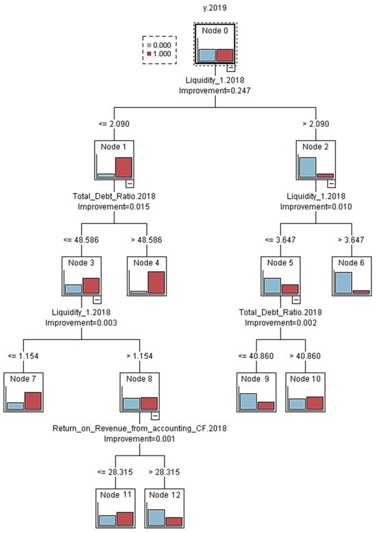
Figure 1. CART model for the Pre-pandemic period (Source: own elaboration).

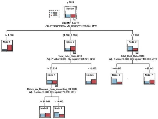
Figure 2. CHAID model for the pre-pandemic period (Source: own elaboration).

In the CART model, the first dividing criterion is Liquidity 1. Companies with Liquidity 1 at or below 2.090 form the left branch, while those with Liquidity 1 above 2.090 form the right branch. On the left branch, the next split is Total Debt Ratio. If the Total Debt Ratio exceeds 48.586, the segment shifts toward higher risk even without further splits. If the Total Debt Ratio is at or below 48.586, the model splits again by Liquidity 1 at 1.154. Values at or below 1.154 indicate a high-risk segment characterised by a predominance of distressed firms. For Liquidity 1 above 1.154, the last distribution is Return on Revenue from accounting Cash Flow, where values at or below 28.315 indicate a higher likelihood of distress, and lower values are linked to a higher share of stable companies. On the right side of the tree, node 2 is split again according to Liquidity 1, with a threshold value of 3.647. Companies with Liquidity 1 higher than 3.647 are immediately classified into the group of stable companies, whereas those with Liquidity 1 in the interval $\left(2.090\right.;\left.3.647\right]$, the Total debt ratio becomes crucial. Among these companies, those with debts of less than 40.860 are classified as stable, while those with higher debts are predominantly distressed.

In the CHAID model, the first dividing criterion is again the Liquidity 1 indicator. Companies with a Liquidity 1 value of 1.078 or lower are classified as high-risk, primarily comprising distressed companies. The remaining companies with liquidity between 1.078 and 2.090 are further split by Total Debt Ratio. If it is at most 32.835, the next division considers Return on Revenue from accounting Cash Flow. A value of up to 19.946 indicates a higher likelihood of distress, while a value above is associated with a higher proportion of stable companies. If the Total Debt Ratio exceeds 32.835 in the moderate liquidity group, the proportion of distressed companies rises even if other liquidity measures are acceptable. For companies with high liquidity (Liquidity 1 above 2.090) the Total Debt Ratio becomes a key factor again. A value of up to 48.442 typically corresponds to a segment mainly composed of stable companies. However, if the Total Debt Ratio exceeds 48.442, the risk of distress increases despite high liquidity. Based on the ranking, short-term liquidity is identified as the most important factor, followed by total debt, with Return on Revenue from Accounting Cash Flow serving as a supporting indicator.

Table 4 presents the results for the pandemic period. Although the models slightly decreased their prediction performance, this may be attributed to the increased economic uncertainty caused by the COVID-19 pandemic. However, it is notable that the DA model has improved compared to its pre-pandemic performance. The CHAID model maintained its high performance, achieving the highest AUC, which highlights its robustness across various economic environments. The neural network achieved the highest sensitivity and the highest accuracy among the compared methods. CART delivered solid accuracy with a stable AUC, and C5.0 performed competitively as well. Logistic regression showed moderate and relatively stable results, but it still lagged behind the tree-based and NN approaches.

Table 4. Performance of prediction models in the pandemic period (Source: own elaboration).

Modelling Technique	Positives		Negatives		Sensitivity (%)	Accuracy (%)	AUC
	TP	FP	FN	TN
CART	35,535	1489	6913	10,264	83.7	84.5	0.88
ANN	36,715	2532	5732	9221	86.5	84.8	0.89
CHAID	35,575	1518	6873	10,235	83.8	84.5	0.92
DA	23,078	5331	19,370	6422	54.4	54.4	0.57
LR	30,586	1111	11,861	10,642	72.1	76.1	0.88
C5.0	35,989	1942	6459	9811	84.8	84.5	0.85

When the models are compared in terms of their evaluation measures, it can be concluded that ANN achieves the highest prediction performance, followed by the CHAID model. Nevertheless, as the ANN model is of a black-box nature, a detailed description of it cannot be provided. However, the importance of the predictors used in this model can be presented. Figure 3 illustrates these details for the six most important variables included in the model, ordered by their predictor importance. The total importance of all predictors in the model is one.

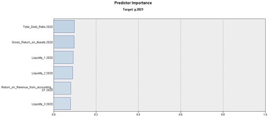
Figure 3. Importance of predictors in the ANN model for the pandemic period (Source: own elaboration).

In this case, the Total Debt Ratio and Gross Return on Assets share first place, with an importance of 0.10, followed by Liquidity 1 and Liquidity 2, with an importance of 0.09. The third place belongs to the Return on Revenue from Accounting Cash Flow and Liquidity 3, with the importance of 0.08.

Figure 4 presents the CHAID model for the pandemic period.

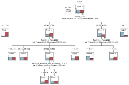
Figure 4. CHAID model for the pandemic period (Source: own elaboration).

As in the pre-pandemic period, the Liquidity 1 indicator maintained its position as the first dividing criterion in the CHAID tree. Companies with a liquidity value of 1.248 or less are classified as high risk and are mostly in distress. The remaining companies with liquidity between 1.248 and 2.379 are further split by the Total Debt Ratio. If the Total Debt Ratio is at most 20.162, the segment is mostly stable. If the total debt ratio is 20.162 or less, the segment is mostly stable with a slight occurrence of blue cases. On the contrary, values between 20.162 and 31.122 show a slight predominance of problematic companies, indicating a slight move towards higher risk. Suppose the Total Debt Ratio is between 31.122 and 46.535. In that case, the next split considers the Return on Revenue from accounting Cash Flow, where a value below 14.951 indicates a higher probability of distress, and a value above 14.951 indicates a higher proportion of stable companies. When the Total Debt Ratio exceeds 46.535 in this group, the proportion of companies in difficulty increases. For companies with higher liquidity, meaning liquidity between 1 and 2.379 and 4.129, the total debt ratio again becomes crucial. A value of up to 46.535 typically corresponds to a segment comprising mostly stable companies, while values above this level increase the risk of distress. At very high liquidity above 4.129, the resulting segment is generally favourable.

In Table 5, which reflects the post-pandemic period, results indicate a partial recovery in performance for most methods. The CHAID model achieved the highest accuracy, confirming its strong overall balance. The CART model achieved the highest sensitivity and maintained a close accuracy. The neural network performed competitively across all metrics, maintaining stable accuracy. Logistic regression achieved the lowest sensitivity yet still yielded a relatively high AUC. The C5.0 tree delivered solid results, and discriminant analysis improved compared with the pandemic period but remained the least effective, particularly in identifying distressed firms. When ranking the models based on all their evaluation measures, the CHAID model should be considered the one with the highest predictive performance. Therefore, Figure 5 presents the CHAID model for the post-pandemic period.

Table 5. Performance of Prediction Models in the post-pandemic period (Source: own elaboration).

Modelling Technique	Positives		Negatives		Sensitivity (%)	Accuracy (%)	AUC
	TP	FP	FN	TN
CART	36,452	1848	6065	10,651	85.7	85.6	0.86
ANN	36,409	2891	6106	9608	85.6	83.7	0.89
CHAID	36,349	1729	6168	10,770	85.5	85.7	0.93
DA	34,171	8583	8346	3916	80.4	69.2	0.58
LR	33,679	1372	8836	11,127	79.2	81.4	0.90
C5.0	35,952	1933	6565	10,566	84.6	84.6	0.85

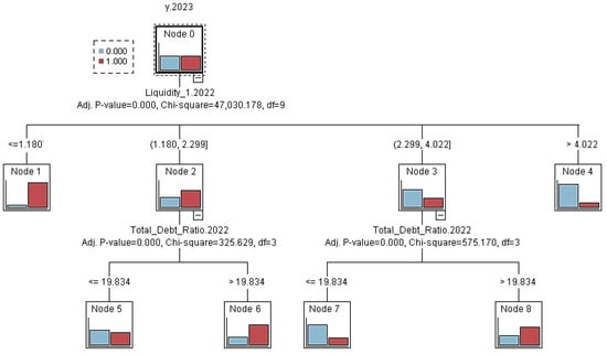
Figure 5. CHAID model for the post-pandemic period (Source: own elaboration).

Comparing the model rankings based on their evaluation measures, we can conclude that CHAID achieves the highest predictive performance. Figure 5 shows the resulting classification tree, including the nodes and the criteria used to divide them.

In the CHAID model, the first dividing criterion is again the Liquidity 1 indicator. Companies with a liquidity value of 1.180 or less are classified as high risk and are mostly in distress. The remaining companies with liquidity between 1.180 and 2.299 are further split by the Total Debt Ratio. If the Total Debt Ratio is at most 19.834, the segment is generally stable; however, values above 19.834 are associated with a higher proportion of distressed firms. For companies with liquidity between 2.299 and 4.022, the total debt ratio becomes crucial again. A debt level of 19.834 or lower indicates a segment dominated by stable companies, while a level above 19.834 increases the risk of distress. With very high liquidity above 4.022, the resulting segment is generally favourable, with a dominance of stable companies.

Table 6 summarises the results of the complex model trained on data covering all periods. Discriminant analysis performed worst across all measurements. The CHAID model again achieved the highest AUC value and high accuracy and sensitivity, confirming its top performance. The CART model and the neural network also achieved very good results, combining high sensitivity with solid accuracy. The C5.0 tree was the weakest among the tree models, but its results remained competitive and at a good level. Clearly, the performance of this comprehensive model was not significantly different from the separate models. This suggests that one comprehensive model can be as effective as individual, economically specific models. In this case, across all evaluation metrics, CART should be considered the most effective method, while DA is the least effective.

Table 6. Performance of the Comprehensive Prediction Models (Source: own elaboration).

Modelling Technique	Positives		Negatives		Sensitivity (%)	Accuracy (%)	AUC
	TP	FP	FN	TN
CART	108,468	5244	17,294	29,148	86.3	85.9	0.87
ANN	107,391	6032	18,369	28,360	85.4	84.8	0.90
CHAID	106,198	4489	19,564	29,903	84.4	85.0	0.92
DA	38,820	8292	86,942	26,100	30.9	40.5	0.56
LR	101,065	4703	24,695	29,689	80.4	81.6	0.90
C5.0	107,142	6144	18,620	28,248	85.2	84.5	0.85

Figure 6 presents the comprehensive CART model for the entire period under review, which has the best predictive properties.

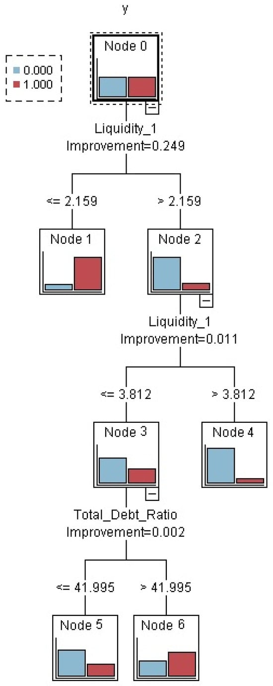
Figure 6. CART comprehensive model for the entire period (Source: own elaboration).

In the CART comprehensive model, the first dividing criterion is also Liquidity 1 indicator. Companies with a Liquidity 1 value at or below 2.159 are classified as high risk, with a dominance of companies in distress. For the remaining companies with Liquidity 1 above 2.159, the tree splits again by Liquidity 1 at 3.812. When Liquidity 1 is at or below 3.812, the next criterion is the Total Debt Ratio. If the Total Debt Ratio is 41.995 or lower, the segment consists mainly of stable companies, whereas values above 41.995 exhibit a higher proportion of companies in difficulty. For companies with high liquidity above 3.812, the resulting segment is generally favourable, with a dominance of stable companies.

Figure 7 presents the CHAID comprehensive model for the entire period under review, which has the second-highest prediction performance.

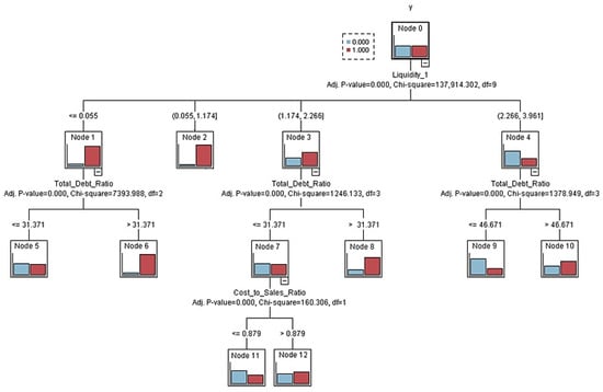
Figure 7. CHAID comprehensive model for the entire period (Source: own elaboration).

In the CHAID model, the first dividing criterion is the Liquidity 1 indicator. Companies with Liquidity 1 equal to or below 0.055 form a separate group, characterised by a higher proportion of companies in difficulty. This group is further divided according to the total debt ratio. When the total debt ratio exceeds 31.371, the segment is clearly dominated by companies in difficulty. When it is at or below 31.371, stable companies dominate. Companies with liquidity 1 in the range of 0.055 to 1.174 form a separate group with an increased proportion of distressed companies. For companies with Liquidity 1 between 1.174 and 2.266, the next split is based on the Total Debt Ratio. If the Total Debt Ratio is 31.371 or lower, the segment is mostly stable. Consequently, it branches according to the Cost-to-Sales Ratio indicator. At values above 0.879, the proportion of companies in difficulty increases, while at values equal to or lower than 0.879, companies without problems dominate. On the contrary, total debt values above 31.371 indicate a segment with a significant number of companies in difficulty. For companies with higher liquidity between 2.266 and 3.961, the Total Debt Ratio becomes decisive again. Debt at or below 46.671 corresponds to a segment dominated by stable firms, whereas debt above 46.671 increases the probability of distress despite higher liquidity.

To supplement the detailed overview of the distribution rules, the key predictors identified by the CART, CHAID, and ANN models in each period are summarised in Table 7. In all decision trees, Liquidity 1 and Total debt ratio are consistently shown as primary distribution variables, while profitability measures such as Return on Revenue from accounting CF are selected as secondary predictors. These recurring patterns suggest that the liquidity position of firms and total debt remain key determinants of financial distress regardless of the economic phase.

Table 7. Main financial predictors of distressed firms (Source: own elaboration).

Period	Model	1st Key Predictor	2nd Key Predictor(s)	3rd Key Predictor(s)
Pre-pandemic	CART	Liquidity 1	Total Debt Ratio; Liquidity 1	Total Debt Ratio; Liquidity
Pre-pandemic	CHAID	Liquidity 1	Total Debt Ratio	Return on Revenue from accounting CF
Pandemic	ANN	Total Debt Ratio	Gross Return on Assets	Liquidity 1
Pandemic	CHAID	Liquidity 1	Total Debt Ratio	Return on Revenue from accounting CF
Post-pandemic	CHAID	Liquidity 1	Total Debt Ratio	-
Comprehensive	CART	Liquidity 1	Liquidity 1	Total Debt Ratio
Comprehensive	CHAID	Liquidity 1	Total Debt Ratio	Cost to Sales Ratio

Comparison of Individual Models and the Comprehensive All-Periods Model

In Table 8, the evaluation of two modelling approaches is summarised: (1) separate models estimated for each period, and (2) a unified comprehensive model estimated on the full sample with a period indicator. The first approach aims to capture phase-specific financial patterns, whereas the second applies a consistent predictive framework across all periods. Across periods, CHAID, CART, and ANN dominate, while DA is clearly the weakest, and LR is consistently average. It is essential to note that the period-indicating variables were not selected as classification criteria in the tree models, indicating their limited additive value for classification purposes. They may be present among the inputs in the ANN, but their high significance has not been proven, and their role cannot be directly interpreted due to the model’s black box nature. The table also shows that the complex model provides the best overall performance. Within this approach, CART achieves the best balance between sensitivity and accuracy, while CHAID is a close competitor, achieving the highest AUC.

Table 8. Performance of modelling techniques across all approaches (Source: own elaboration).

Modelling Technique	Pre-Pandemic			Pandemic			Post-Pandemic			Comprehensive Model
	Sensitivity (%)	Accuracy (%)	AUC	Sensitivity (%)	Accuracy (%)	AUC	Sensitivity (%)	Accuracy (%)	AUC	Sensitivity (%)	Accuracy (%)	AUC
CART	85.8	85.7	0.90	83.7	84.5	0.88	85.7	85.6	0.86	86.3	85.9	0.87
ANN	85.3	84.6	0.90	86.5	84.8	0.89	85.6	83.7	0.89	85.4	84.8	0.90
CHAID	85.3	85.4	0.92	83.8	84.5	0.92	85.5	85.7	0.93	84.4	85.0	0.92
DA	27.1	38.3	0.56	54.4	54.4	0.57	80.4	69.2	0.58	30.9	40.5	0.56
LR	79.3	81.1	0.90	72.1	76.1	0.88	79.2	81.4	0.90	80.4	81.6	0.90
C5.0	85.1	84.4	0.84	84.8	84.5	0.85	84.6	84.6	0.85	85.2	84.5	0.85

Since the CART comprehensive model was identified as the best overall, its performance was cross-evaluated in separate tree periods: pre-pandemic, pandemic, and post-pandemic. This evaluation was performed by comparing the actual state of the companies with the predictions of the comprehensive model, followed by calculating the sensitivity, accuracy, and AUC separately for each period. Table 9 presents these values. Overall, the model’s performance can be considered remarkably stable across periods. Sensitivity varies only slightly, so the small decline during the pandemic is insignificant. Accuracy is virtually unchanged, indicating consistent overall classification quality. AUC remains stable across all periods, and the Gini index is likewise steady, further confirming stable discriminatory power.

Table 9. Performance of the comprehensive CART model in individual periods (Source: own elaboration).

Period	Sensitivity (%)	Accuracy (%)	AUC
Pre-pandemic	87.2	85.8	0.85
Pandemic	85.6	85.6	0.86
Post-pandemic	86.3	85.9	0.86
Entire	96.3	85.9	0.87

4. Discussion

This study examined whether a change in modelling approach improves the prediction of a company’s financial state across different economic periods. We compared period-specific models with a single universal model that included a period indicator. The main finding is that prediction accuracy remained broadly stable across approaches. The universal model matched the performance of period-specific models even during the turbulence associated with the pandemic period. This suggests that well-specified models can absorb regime variation without the need for frequent recalibration. The following section synthesises the models and their performance comparison across the periods.

4.1. Comparative Interpretation of Models’ Performance

The comparative analysis of the modelling techniques reveals clear and consistent differences in their predictive capabilities across the examined economic periods. Non-linear machine learning methods, particularly ANNs and tree-based approaches (CART and CHAID), demonstrated stronger and more stable performance than classical statistical techniques. These findings are in line with previous studies suggesting that flexible, non-parametric learning algorithms adapt more readily to structural breaks and heterogeneous data patterns characteristic of financial distress processes (e.g., Barboza et al., 2017; Zelenkov & Volodarskiy, 2021). Their ability to model non-linear relationships among variables, interactions, and threshold effects gives them an advantage when financial indicators behave differently across varying macroeconomic conditions.

Among all the techniques, the CHAID method achieved the strongest results in terms of sensitivity, overall accuracy, and AUC, while discriminant analysis lagged behind. The strength of the CHAID method lies in its ability to capture non-linear relationships in heterogeneous data. By contrast, DA exhibited the weakest performance across the majority of evaluation metrics. Its weaker performance can be attributed to its restrictive assumptions. DA requires multivariate normality and equal covariance matrices across groups; however, these conditions financial ratios rarely satisfy, particularly during crisis periods. The technique is also sensitive to outliers and, unlike other methods, cannot capture non-linear patterns and variable interactions. These methodological constraints likely contributed to DA achieving the lowest accuracy across most evaluation metrics.

Across the economic periods, no single modelling technique uniformly dominated, but several important patterns emerged. First, the pandemic period produced the largest decline in predictive accuracy across all models, confirming that rapid and unpredictable changes in financial structures pose challenges for estimation and classification. Second, the ranking of models changed slightly between periods, indicating that the relative effectiveness of modelling approaches is sensitive to the economic environment. This finding is consistent with the hypothesis that financial distress processes differ across regimes. Third, the comprehensive model covering all periods produced results comparable to those of many period-specific models, suggesting that a unified approach, supported by a period indicator, can sufficiently absorb cross-period heterogeneity for practical predictive use. Amirshahi and Lahmiri (2024) also demonstrate in their study that ensembles and gradient boosting effectively handle highly imbalanced bankruptcy data, delivering strong accuracy on unseen test sets, which supports the finding of this study that a single flexible model can maintain reliable performance. Rahman and Zhu (2024) also report that modern machine learning models outperform traditional approaches in predicting financial distress in the construction sector, which further aligns with results. However, the superior performance of some period-specific models in certain metrics indicates that full parameter pooling may not always be optimal during highly disrupted conditions.

4.2. Key Findings and Implications of the Study

These findings have practical implications for risk managers, investors, and regulators. A single comprehensive model with a transparent period indicator can provide reliable monitoring without the burden of maintaining separate models for each macroeconomic phase. This simplifies management and supports decision-making. Macro-level evidence complements this view. Acheampong et al. (2024) document international variation in bank credit risk during the COVID-19 period, which supports the use of a simple period indicator to acknowledge shifting risk conditions while keeping the core predictive structure stable. Hu et al. (2025) analyse bank failures over the long term and show that machine learning techniques retain strong predictive power while taking advantage of time-saving controls, which is consistent with the universal model strategy applied in this study.

The results also help explain why performance remained relatively stable during the pandemic. It appears that most of the predictive power comes from company-level indicators, which remain informative over the years, while the period indicator only adjusts to changes in the environment. This suggests that once key financial indicators are correctly specified, a single flexible model can remain effective even under changing macroeconomic conditions. The finding of this study that a single, well-specified universal model performs as well as period-specific specifications is consistent with extensive studies showing that flexible, non-linear methods generally achieve strong performance on unseen test data in the area of credit risk and financial distress prediction. For instance, Lessmann et al. (2015) found that modern classification approaches, especially tree and ensemble methods, outperform traditional techniques in credit scoring, which is consistent with the finding of better performance of tree algorithms compared to discriminant analysis. Similarly, Barboza et al. (2017) show that bagging, boosting, and random forests significantly improve bankruptcy prediction accuracy compared to discriminant analysis and logistic regression, which supports results of this study, in which CHAID outperformed discriminant analysis. However, regarding the time stability of models, the picture in the literature is mixed. Papik and Papikova (2022) documented a noticeable weakening of model performance during periods of crisis, highlighting the need for recalibration, which contrasts with our findings. In contrast, du Jardin (2021) emphasises the contribution of dynamic approaches that explicitly model the evolution of a firm over time to capture regime changes. More recent work also points to the expansion of the feature set, demonstrating the benefits of textual and hybrid approaches. T. Chen et al. (2023) increase accuracy by adding textual information from annual reports to machine learning models. A comprehensive review by Dasilas and Rigani (2024) further concludes that modern machine learning methods generally outperform traditional techniques, which reinforces the consistency of the results presented here.

It is important to acknowledge that although economic phases cannot be forecasted in advance, the purpose of analysis presented in this study is not to identify future economic conditions, nor to predict the future economic phase of the companies, but rather to evaluate how different predictive models behave when economic conditions change significantly. Understanding a model’s robustness across different economic periods provides valuable insights for practitioners operating in uncertain environments. Such evidence helps determine whether a single comprehensive model can be reliably used across heterogeneous environments or whether recalibration is advisable when early signs of economic stress appear.

Although the empirical data used in this study come solely from Slovak companies, the methodological contributions and empirical insights extend beyond national boundaries. Firstly, the modelling approaches used (decision trees, neural networks, logistic regression, and discriminant analysis) are universal and widely applied in corporate finance and risk management worldwide. Secondly, the finding that a single well-specified model can match the performance of period-specific models offers practical value to international practitioners facing similar questions about model recalibration during crises. Then, Slovakia represents an informative and policy-relevant case for investigating model stability across economic conditions. As a small, open, and export-oriented economy with a high share of small and medium-sized enterprises (over 99%), Slovakia exhibits structural characteristics common to many European and global markets. Finally, many structural factors that affect financial distress, such as liquidity shortages, rising debt burdens, or profitability shocks, are not country-specific but shared by SMEs across the continents. Similarly to many other countries, Slovak companies experienced the full spectrum of economic conditions during the study period: a stable pre-pandemic phase, an intense COVID-19 shock, and a post-pandemic recovery, nevertheless marked by inflationary pressures and supply chain disruptions. Therefore, evidence from Slovakia contributes to a broader understanding of how predictive models behave under economic stress and provides insights relevant to modelling in other countries.

5. Conclusions

This study examined how a change in modelling approach impacts the ability to predict a company’s financial state across different economic periods. Our findings indicate no significant differences in prediction accuracy across the individual periods compared to the comprehensive universal model for all periods. Even though the economic disruptions caused by the COVID-19 pandemic significantly affect companies’ financial performance, the use of a period-specific model, or at least a period indicator variable, helps maintaining the models’ predictive accuracy.

Hypothesis H1, which assumed that the relative ranking of the predictive performance of modelling techniques would be significantly varied across economic periods, was therefore only partially supported. During the pandemic, a significant improvement in discriminant analysis was observed compared to the periods before and after, while the performance of other methods changed only slightly, leaving the overall ranking largely stable across periods. Hypothesis H2 was not supported, as the period-specific models did not achieve higher accuracy than a comprehensive model that included a period indicator. Across all techniques evaluated, CHAID slightly outperformed other models in terms of sensitivity, accuracy, and AUC, while discriminant analysis consistently showed the lowest predictive performance. These results suggest that a robustly constructed complex model can offer equally reliable predictive accuracy and provide a simpler yet practically beneficial approach. As a result, practitioners, investors, and regulators can confidently apply such complex models, even during periods of economic uncertainty.

This study also has several limitations that suggest directions for further research. First, the models were evaluated by using the 50:50 train–test split. In the future, the performance of the models created in this study should be evaluated using either a cross-validation technique or by verifying the accuracy of their predictions on newly generated data from consecutive years. Second, missing values in the financial ratios were imputed with industry averages, which may weaken variability and relationships between variables. In further research, more advanced imputation methods, such as model-based imputation, could help mitigate the bias caused by the imputation. Third, the modelling framework does not specify the causal relationships between a company’s financial state and financial indicators or their structural interactions with pandemic-related effects. Instead, these interdependencies are absorbed implicitly through the financial ratios and the COVID-19 dummy variable. While this approach is appropriate for predictive modelling, it does not capture the theoretical directionality of financial relationships, which represents a methodological limitation. Then, although we compared six popular techniques (CART, CHAID, C5.0, ANN, LR, DA), we did not explore more complex techniques, such as ensemble modelling, gradient boosting, or hybrid models, which often improve performance but are often hindered by their low readability. Next, the models are one year ahead, and in this study, they are purposely prioritised for predictive performance over interpretability. After that, the set of potential financial distress predictors consists exclusively of firm-level ratios. Adding macroeconomic and sectoral covariates, such as demand shocks and policy measures, and their interaction with firm characteristics, could shed light on why performance remains stable across periods and whether there is heterogeneity by size or industry. Furthermore, classifying 2022–2023 as a post-pandemic period is an oversimplification. These years were still affected by major macroeconomic shocks, notably the war in Ukraine, rising energy prices, and high inflation. Therefore, the post-pandemic period in this study should be interpreted as a phase with overlapping shocks rather than a completely stable regime, and future research could refine the periodisation or explicitly model multiple concurrent shocks to verify the robustness of the results. Another limitation is the very high variability and extreme values observed in some financial indicators. These wide ranges are caused by companies with extreme but economically acceptable indicator values, which are typical for populations of small and medium-sized enterprises with small denominators, large losses, or one-off gains. In the environment of SMEs, even slight changes in income, assets, or liabilities can translate into very large movements in financial ratios, so such variability does not usually indicate errors in the data but rather reflects the underlying financial reality. In addition, extreme values may signal emerging financial distress and therefore provide essential information for predictive modelling. Removing these observations would eliminate precisely the type of signals that financial distress models seek to detect and would bias the sample toward financially stable firms. In this study, only observations with economically inconsistent or technically incorrect values in mandatory items were removed, while extreme but acceptable indicator values were retained, and no winsorisation or robust transformation of indicators were used. As a result, the reported standard deviations remain high, and future research could use alternative scaling, trimming, or winsorisation procedures to assess the sensitivity of the models to such extremes. Finally, our findings are most closely related to Slovak SMEs. Replication in other countries, legal environments, and with alternative definitions of distress would test the transferability and boundary conditions.

References

- Acheampong, A., Ibeji, N., & Danso, A. (2024). COVID-19 and credit risk variation across banks: International insights. Managerial and Decision Economics, 45(7), 4415–4431. [Google Scholar] [CrossRef]
- Alam, T. M., Shaukat, K., Mushtaq, M., Ali, Y., Khushi, M., Luo, S., & Wahab, A. (2021). Corporate bankruptcy prediction: An approach towards better corporate world. The Computer Journal, 64(11), 1731–1746. [Google Scholar] [CrossRef]
- Altman, E. I. (1968). Financial ratios, discriminant analysis and the prediction of corporate bankruptcy. Journal of Finance, 23(4), 589–609. [Google Scholar] [CrossRef]
- Amankwah-Amoah, J., Khan, Z., & Wood, G. (2021). COVID-19 and business failures: The paradoxes of experience, scale, and scope for theory and practice. European Management Journal, 39(2), 179–184. [Google Scholar] [CrossRef] [PubMed]
- Amirshahi, B., & Lahmiri, S. (2024). Bankruptcy prediction using optimal ensemble models under balanced and imbalanced data. Expert Systems, 41(8), e13599. [Google Scholar] [CrossRef]
- Archanskaia, E., Canton, E., Hobza, A., Nikolov, P., & Simons, W. (2023). The asymmetric impact of COVID-19: A novel approach to quantifying financial distress across industries. European Economic Review, 158, 104509. [Google Scholar] [CrossRef] [PubMed]
- Aydin, N., Sahin, N., Deveci, M., & Pamucar, D. (2022). Prediction of financial distress of companies with artificial neural networks and decision trees models. Machine Learning with Applications, 10, 100432. [Google Scholar] [CrossRef]
- Balina, R., Idasz-Balina, M., & Achsani, N. A. (2021). Predicting insolvency of the construction companies in the creditworthiness assessment process—Empirical evidence from Poland. Journal of Risk and Financial Management, 14(10), 453. [Google Scholar] [CrossRef]
- Barboza, F., Kimura, H., & Altman, E. (2017). Machine learning models and bankruptcy prediction. Expert Systems with Applications, 83, 405–417. [Google Scholar] [CrossRef]
- Beaver, W. H. (1966). Financial ratios as predictors of failure. Journal of Accounting Research, 4, 71–111. [Google Scholar] [CrossRef]
- Bobitan, N., & Dumitrescu, D. (2024). Financial distress of Romanian listed companies under systemic events: Analysis and accuracy of prediction models. Transformations in Business & Economics, 23(1), 305–324. [Google Scholar]
- Box, G. E. P., & Jenkins, G. M. (1970). Time series analysis: Forecasting and control. Holden-Day. [Google Scholar]
- Box, G. E. P., Jenkins, G. M., Reinsel, G. C., & Ljung, G. M. (2016). Time series analysis: Forecasting and control (5th ed.). Wiley. [Google Scholar]
- Bozkurt, İ., & Kaya, M. V. (2023). Foremost features affecting financial distress and bankruptcy in the acute stage of COVID-19 crisis. Applied Economics Letters, 30(8), 1112–1123. [Google Scholar] [CrossRef]
- Breiman, L., Friedman, J. H., Olshen, R. A., & Stone, C. J. (1984). Classification and regression trees. Wadsworth. [Google Scholar]
- Chakrabarti, B., Jain, A., Nagpal, P., & Rout, J. K. (2024). A spatiotemporal context aware hierarchical model for corporate bankruptcy prediction. Multimedia Tools and Applications, 83(10), 28281–28303. [Google Scholar] [CrossRef]
- Chatfield, C. (2003). The analysis of time series: An introduction (6th ed.). Chapman & Hall/CRC. [Google Scholar]
- Chen, M.-Y. (2011). Predicting corporate financial distress based on integration of decision tree classification and logistic regression. Expert Systems with Applications, 38(9), 11261–11272. [Google Scholar] [CrossRef]
- Chen, T., Liao, H., Chen, G., Kang, W., & Lin, Y. (2023). Bankruptcy prediction using machine learning models with the text-based communicative value of annual reports. Expert Systems with Applications, 233, 120714. [Google Scholar] [CrossRef]
- Citterio, A. (2024). Bank failure prediction models: Review and outlook. Socio-Economic Planning Sciences, 92, 101818. [Google Scholar] [CrossRef]
- Das, R. C. (2020). Forecasting incidences of COVID-19 using Box-Jenkins method for the period July 12–September 11, 2020: A study on highly affected countries. Chaos, Solitons & Fractals, 140, 110248. [Google Scholar]
- Dasilas, A., & Rigani, A. (2024). Machine learning techniques in bankruptcy prediction: A systematic literature review. Expert Systems with Applications, 255, 124761. [Google Scholar] [CrossRef]
- Dieperink, H., Adriaanse, J., & Dechesne, M. (2024). Predicting viability of small businesses on the edge of failure. Journal of Small Business Management, 63(5), 2422–2454. [Google Scholar] [CrossRef]
- Dubea, F., Nzimande, N., & Muzindutsi, P.-F. (2021). Application of artificial neural networks in predicting financial distress in the JSE financial services and manufacturing companies. Journal of Sustainable Finance & Investment, 13(1), 723–743. [Google Scholar] [CrossRef]
- du Jardin, P. (2021). Dynamic self-organizing feature map-based models applied to bankruptcy prediction. Decision Support Systems, 147, 113576. [Google Scholar] [CrossRef]
- Durana, P., Kovalova, E., Blazek, R., & Bicanovska, K. (2025a). Business efficiency: Insights from Visegrad four before, during, and after the COVID-19 pandemic. Economies, 13(2), 26. [Google Scholar] [CrossRef]
- Durana, P., Poliak, M., Kovalova, E., & Blazek, R. (2025b). Prediction models reloaded: Advanced insights for SMEs in the Bucharest Nine countries. Oeconomia Copernicana, 16(2), 689–760. [Google Scholar] [CrossRef]
- Durica, M., Frnda, J., & Svabova, L. (2019). Decision tree based model of business failure prediction for Polish companies. Oeconomia Copernicana, 10(3), 453–469. [Google Scholar] [CrossRef]
- Durica, M., Svabova, L., & Kramarova, K. (2023, September 28–29). Predictive modelling of financial distress of Slovak companies using machine learning techniques. 8th International Scientific Conference of the Economics, Management & Business (pp. 780–786), High Tatras, Slovakia. [Google Scholar]
- Elsayed, N., Elaleem, S. A., & Marie, M. (2024). Improving prediction accuracy using random forest algorithm. International Journal of Advanced Computer Science and Applications, 15(4), 436–441. [Google Scholar] [CrossRef]
- Gabrikova, B., Svabova, L., & Kramarova, K. (2023). Machine learning ensemble modelling for predicting unemployment duration. Applied Sciences, 13(18), 10146. [Google Scholar] [CrossRef]
- Goodfellow, I., Bengio, Y., & Courville, A. (2016). Deep learning. MIT Press. [Google Scholar]
- Halteh, K. (2025). Does size matter? Analysing the financial implications of COVID-19 on SMEs and large companies using a hybrid methodology. Journal of Statistical Theory and Applications, 24, 199–217. [Google Scholar] [CrossRef]
- Hammond, P., Opoku, M. O., Kwakwa, P. A., & Amissah, E. (2023). Predictive models of going concerns and business failure. Cogent Business & Management, 10(2), 2226481. [Google Scholar] [CrossRef]
- Haykin, S. (1999). Neural networks: A comprehensive foundation (2nd ed.). Prentice Hall. [Google Scholar]
- Hosmer, D. W., Lemeshow, S., & Sturdivant, R. X. (2013). Applied logistic regression (3rd ed.). Wiley. [Google Scholar]
- Hu, W., Shao, C., & Zhang, W. (2025). Predicting U.S. bank failures and stress testing with machine learning algorithms. Finance Research Letters, 75, 106802. [Google Scholar] [CrossRef]
- Huberty, C. J., & Olejnik, S. (2006). Applied MANOVA and discriminant analysis (2nd ed.). Wiley. [Google Scholar]
- Hyndman, R. J., & Athanasopoulos, G. (2018). Forecasting: Principles and practice (2nd ed.). OTexts. [Google Scholar]
- Jang, Y., Jeong, I., Cho, Y., & Ahn, Y. (2019). Predicting business failure of construction contractors using long short-term memory recurrent neural network. Journal of Construction Engineering and Management, 145(11), 04019067. [Google Scholar] [CrossRef]
- Johnson, R. A., & Wichern, D. W. (2008). Multivariate analysis. In F. Ruggeri, R. S. Kenett, & F. W. Faltin (Eds.), Encyclopedia of statistics in quality and reliability. Wiley. [Google Scholar]
- Kaczmarek, J. (2012). Construction elements of bankruptcy prediction models in multi-dimensional early warning systems. Polish Journal of Management Studies, 5, 130–143. [Google Scholar]
- Kass, G. V. (1980). An exploratory technique for investigating large quantities of categorical data. Journal of the Royal Statistical Society: Series C (Applied Statistics), 29(2), 119–127. [Google Scholar] [CrossRef]
- Khashei, M., Etemadi, S., & Bakhtiarvand, N. (2024). A new discrete learning-based logistic regression classifier for bankruptcy prediction. Wireless Personal Communications, 134(2), 1075–1092. [Google Scholar]
- Kicova, E., Svabova, L., Ponisciakova, O., & Rosnerova, Z. (2025). Forecasting financial literacy levels with respect to consumer shopping behaviour. International Journal of Financial Studies, 13(1), 1. [Google Scholar] [CrossRef]
- Kitowski, J., Kowal-Pawul, A., & Lichota, W. (2022). Identifying symptoms of bankruptcy risk based on bankruptcy prediction models—A case study of Poland. Sustainability, 14(3), 1416. [Google Scholar] [CrossRef]
- Lachenbruch, P. A. (2006). Discriminant analysis. In S. Kotz, C. B. Read, N. Balakrishnan, B. Vidakovic, & N. L. Johnson (Eds.), Encyclopedia of statistical sciences. Springer. [Google Scholar]
- Laitinen, E. K., Camacho-Minano, M. D., & Munoz-Izquierdo, N. (2023). A review of the limitations of financial failure prediction research. Revista de Contabilidad—Spanish Accounting Review, 26(2), 255–273. [Google Scholar] [CrossRef]
- Lessmann, S., Baesens, B., Seow, H., & Thomas, L. C. (2015). Benchmarking state-of-the-art classification algorithms for credit scoring: An update of research. European Journal of Operational Research, 247(1), 124–136. [Google Scholar] [CrossRef]
- Loh, W. Y. (2011). Classification and regression trees. Wiley Interdisciplinary Reviews: Data Mining and Knowledge Discovery, 1(1), 14–23. [Google Scholar]
- Long, J. S. (1997). Regression models for categorical and limited dependent variables. SAGE Publications. [Google Scholar]
- Magidson, J. (1993). The CHAID approach to segmentation modelling: Chi-squared automatic interaction detection. In R. P. Bagozzi (Ed.), Advanced methods of marketing research (pp. 118–159). Blackwell. [Google Scholar]
- Massahi Khoraskani, M., Kheradmand, F., & Arshadi Khamseh, A. (2018). Application and comparison of neural network, C5.0, and classification and regression trees algorithms in the credit risk evaluation problem (case study: A standard German credit dataset). International Journal of Knowledge Engineering and Data Mining, 4(1), 259–276. [Google Scholar] [CrossRef]
- Mate, D., Raza, H., & Ahmad, I. (2023). Comparative analysis of machine learning models for bankruptcy prediction in the context of Pakistani companies. Risks, 11(10), 176. [Google Scholar] [CrossRef]
- Menard, S. (2002). Applied logistic regression analysis (2nd ed.). SAGE Publications. [Google Scholar]
- Narvekar, A., & Guha, D. (2021). Bankruptcy prediction using machine learning and an application to the case of the COVID-19 recession. Data Science in Finance and Economics, 1(2), 180–195. [Google Scholar] [CrossRef]
- Papik, M., & Papikova, L. (2022). Impacts of crisis on SME bankruptcy prediction models’ performance. Expert Systems with Applications, 214, 119072. [Google Scholar] [CrossRef]
- Papik, M., & Papikova, L. (2024). Automated machine learning in bankruptcy prediction of manufacturing companies. Procedia Computer Science, 232, 1428–1436. [Google Scholar] [CrossRef]
- Peng, C. Y. J., Lee, K. L., & Ingersoll, G. M. (2002). An introduction to logistic regression analysis and reporting. The Journal of Educational Research, 96(1), 3–14. [Google Scholar] [CrossRef]
- Rahman, M. J., & Zhu, H. (2024). Predicting financial distress using machine learning approaches: Evidence China. Journal of Contemporary Accounting & Economics, 20(1), 100403. [Google Scholar] [CrossRef]
- Rencher, A. C., & Christensen, W. F. (2012). Methods of multivariate analysis (3rd ed.). Wiley. [Google Scholar] [CrossRef]
- Rudd Mph, G. J., & Priestley, J. L. (2017). A comparison of decision tree with logistic regression model for prediction of worst non-financial payment status in commercial credit. Grey Literature from PhD Candidates, 5. Available online: http://digitalcommons.kennesaw.edu/dataphdgreylit/5 (accessed on 3 March 2025).
- Shetty, S., Musa, M., & Brédart, X. (2022). Bankruptcy prediction using machine learning techniques. Journal of Risk and Financial Management, 15(1), 35. [Google Scholar] [CrossRef]
- Shi, Y., & Li, X. (2024). Bankruptcy prediction for the European aviation industry: An application of the Altman model. Managerial and Decision Economics, 45(1), 477–491. [Google Scholar] [CrossRef]
- Song, Y. Y., & Lu, Y. (2015). Decision tree methods: Applications for classification and prediction. Shanghai Archives of Psychiatry, 27(2), 130–135. [Google Scholar]
- Soni, R. (2019). Application of discriminant analysis to diagnose the financial distress. Theoretical Economics Letters, 9(4), 1197–1209. [Google Scholar] [CrossRef]
- Spiler, M., Matejic, T., Knezevic, S., Milasinovic, M., Mitrovic, A., Arsic, V. B., Obradovic, T., Simonovic, D., Despotovic, V., Milojevic, S., Adamovic, M., Resimic, M., & Milosevic, P. (2022). Assessment of the bankruptcy risk in the hotel industry as a condition of the COVID-19 crisis using time-delay neural networks. Sustainability, 15(1), 272. [Google Scholar] [CrossRef]
- Svabova, L., Kramarova, K., & Chabadova, D. (2022). Impact of the COVID-19 pandemic on the business environment in Slovakia. Economies, 10(10), 244. [Google Scholar] [CrossRef]
- Valaskova, K., Gajdosikova, D., & Belas, J. (2023). Bankruptcy prediction in the post-pandemic period: A case study of Visegrad group countries. Oeconomia Copernicana, 14(1), 253–293. [Google Scholar] [CrossRef]
- Vlaović Begović, S., & Bonić, L. (2020). Developing a model to predict corporate bankruptcy using decision tree in the Republic of Serbia. Facta Universitatis, Series: Economics and Organization, 17(2), 127–139. [Google Scholar] [CrossRef]
- Wu, D., Ma, X., & Olson, D. L. (2022). Financial distress prediction using integrated Z-score and multilayer perceptron neural networks. Decision Support Systems, 159, 113814. [Google Scholar] [CrossRef]
- Yakymova, L., & Kuz, V. (2019). The use of discriminant analysis in the assessment of municipal company’s financial health. Economics & Sociology, 12(2), 64–78. [Google Scholar]
- Zelenkov, Y., & Volodarskiy, N. (2021). Bankruptcy prediction on the base of the unbalanced data using multi-objective selection of classifiers. Expert Systems with Applications, 185, 115559. [Google Scholar] [CrossRef]
- Zizi, Y., Jamali-Alaoui, A., El Goumi, B., Oudgou, M., & El Moudden, A. (2021). An optimal model of financial distress prediction: A comparative study between neural networks and logistic regression. Risks, 9(11), 200. [Google Scholar] [CrossRef]
Disclaimer/Publisher’s Note: The statements, opinions and data contained in all publications are solely those of the individual author(s) and contributor(s) and not of MDPI and/or the editor(s). MDPI and/or the editor(s) disclaim responsibility for any injury to people or property resulting from any ideas, methods, instructions or products referred to in the content. |
© 2025 by the authors. Licensee MDPI, Basel, Switzerland. This article is an open access article distributed under the terms and conditions of the Creative Commons Attribution (CC BY) license (https://creativecommons.org/licenses/by/4.0/).