Article

Statistical Quantification of the COVID-19 Pandemic’s Continuing Lingering Effect on Economic Losses in the Tourism Sector

by
Amos Mohau Mphanya
1,
Sandile Charles Shongwe
1,*,
Thabiso Ernest Masena
2 and
Frans Frederick Koning
1
1
Department of Mathematical Statistics and Actuarial Science, Faculty of Natural and Agricultural Sciences, University of the Free State, Bloemfontein 9301, South Africa
2
Department of Mathematics and Applied Mathematics, Faculty of Natural and Agricultural Sciences, University of the Free State (South Campus), Bloemfontein 9301, South Africa
*
Author to whom correspondence should be addressed.
Economies 2025, 13(12), 362; https://doi.org/10.3390/economies13120362
Submission received: 17 October 2025 / Revised: 12 November 2025 / Accepted: 24 November 2025 / Published: 9 December 2025
(This article belongs to the Section Economic Development)

Abstract

The impact of the COVID-19 pandemic on the number of international tourist arrivals in the Republic of South Africa (RSA) is studied in this paper using the seasonal autoregressive integrated moving average (SARIMA) model comprising a pulse function covariate vector evaluated via trial and error as an exogenous variable (SARIMAX). This paper provides a methodological innovation that combines outlier detection with intervention quantification so that tourism academics and practitioners can correctly capture estimated economic losses caused by the COVID-19 pandemic and the response to it. In the pre-intervention modelling, four additive outliers and innovative outliers were detected and incorporated into the SARIMAX ( 1 , 1 , 1 ) ( 0 , 1 , 2 ) 12 model, which significantly lowered the model’s evaluation metrics, making it the best fitting pre-intervention model. Next, from March 2020 to June 2025 (end of dataset), it is shown that the estimated total losses amount to 7,328,919 tourists compared to if there been no pandemic. This means that the number of tourist arrivals in the RSA has not yet returned to the pre-COVID-19 forecasted path as of June 2025, indicating that the COVID-19 pandemic continues to have long-term negative effects on the RSA’s number of tourist arrivals. Therefore, more efforts must be focused on developing innovative and advanced statistical models to assist the RSA government and private entities in creating incentives for investment, planning more effectively, providing societies reliant on tourism with more resources, and creating suitable regulations that boost the economy through the tourism sector.

1. Introduction and Literature Review

It is unarguable that the tourism sector has been the largest contributor to the global and African economies for a long time due to its significantly positive contribution towards economic growth and development through job creation (Viljoen et al., 2019). Naudé and Saayman (2005) even referred to Africa as a continent of explorers and adventures. However, this significant progress towards the improvement of sustainable economies through various channels within the tourism sector was hampered by the emergence of the 2019 novel coronavirus (COVID-19) pandemic in 2020. As a result, the RSA (Republic of South Africa) government responded with strict measures and protocols, which included extreme or strict restrictions on local and international travel (Rogan & Skinner, 2020). A multitude of studies have pointed out that the tourism sector was the hardest hit globally due to its heavy reliance on tourist arrivals and the physical nature of its activities (Ilo et al., 2023). A. Liu et al. (2021) asserted that the COVID-19 pandemic has caused a significant decline in South Africa’s international tourist arrivals and foreign tourist income. Additional studies on the social and economic impact of the COVID-19 pandemic in the RSA and the other parts of the world can be found in the works by Ilo et al. (2023), Hamza et al. (2025), Zenker and Kock (2020), and Demir et al. (2021).
To the authors’ knowledge, there exist only three time series analysis studies aimed at investigating the sustained impact of the COVID-19 pandemic in the RSA using tourist arrivals data (see Chipumuro and Chikobvu (2022) and Chipumuro et al. (2024a, 2024b)). All three of these papers assessed the impact of COVID-19 on the number of monthly international tourist arrivals from other countries to the RSA using the Box–Jenkins’ seasonal autoregressive integrated moving average (SARIMA) models outlined in Cryer and Chan (2008). The studies by Chipumuro and Chikobvu (2022) and Chipumuro et al. (2024a, 2024b) concluded that before the emergence of COVID-19, the number of tourist arrivals in the RSA showed a sustained upward trend and seasonality but were negatively affected immediately after the onset of the COVID-19 pandemic. However, the following inconsistencies and deficiencies were noted within Chipumuro and Chikobvu (2022) and Chipumuro et al. (2024a, 2024b):
(i)
The three studies did not provide the estimated loss of tourist arrivals in the post-intervention period;
(ii)
The selected pre-intervention period in the three studies is inconsistent with the exact timeframe (March 2020) in which lockdown was introduced in RSA;
(iii)
The different types of outliers were not detected in the three studies and incorporated within the pre-intervention model in order to improve its overall fit and accuracy;
(iv)
The three studies used basic SARIMA models without incorporating any intervention variables to capture the effect of COVID-19 during the post-intervention period, meaning that we may quantify the exact economic losses due to the sustained negative effect (or lingering effect) of the COVID-19 pandemic since March 2020 when the first strict lockdown was implemented in the RSA.
In tourism analysis applied to data from other countries, different researchers have used various time series methodologies to study the impact of the COVID-19 pandemic within those tourism sectors, depending on the dynamics observed within those particular data. For instance, Arshad et al. (2021) investigated the loss of monthly foreign tourist arrivals caused by COVID-19 in the Indian tourism industry. Their study used the SARIMA and Holt–Winters models to accurately capture and forecast the expected foreign tourist arrivals in India from March 2020 to December 2020. Both the SARIMA and Holt–Winters models accounted for trends and seasonality in this study, but losses in foreign tourist arrivals were not quantified and the outlier detection analysis was not conducted before fitting the models. This study found that the SARIMA model outperformed the Holt–Winters method and the onset of COVID-19 caused an enormous reduction in the number of expected foreign tourist arrivals in India.
In a similar study, Paudel et al. (2024) investigated the monthly patterns of international tourist arrivals in Nepal from January 1992 to December 2023, where they implemented the SARIMA and Holt–Winters exponential smoothing (Winters additive and multiplicative) models to assess the impact of earthquake in 2015 and COVID-19 in 2020 to Nepal tourism industry. The Winters additive and multiplicative model outperformed the SARIMA model, displaying the lowest error metric values. This study found that the number of tourist arrivals would have continued to increase in Nepal had the earthquake and the COVID-19 pandemic not occurred. Janjua et al. (2021) investigated the impact of COVID-19 on the inflow of international tourists into Thailand from January 1991 to March 2020 using the autoregressive integrated moving average (ARIMA) model. This study found that the COVID-19 pandemic caused a shortfall in international tourist arrivals in Thailand, which had not returned to their pre-intervention levels by December 2020.
Rahayu and Sumargo (2023) assessed the impact of the COVID-19 pandemic on the number of foreign tourists visiting Indonesia from January 2016 to July 2021. Their study used ARIMA and autoregressive conditional heteroscedasticity (ARCH) to model the dataset and revealed that the number of foreign tourists visiting Indonesia declined due to the emergence of COVID-19, which also decreased tourism income. Devi et al. (2024) investigated the number of international tourist arrivals before and after the onset of COVID-19 in the Indian tourism industry. Their study used a yearly pre-pandemic international tourist arrivals dataset from January 1995 to December 2019 and a post-pandemic series from January 2022 to November 2023 in India. Devi et al. (2024) fitted the ARIMA and SARIMA models and found that during the pre-intervention period, tourist arrivals in India increased significantly, while the onset of COVID-19 caused a decline in tourist arrivals; in addition, they also observed that from February 2022, tourist arrivals gradually returned to their original baseline.
Khusna et al. (2024) monitored the number of monthly international tourist arrivals entering Soekarno-Hatta, Ngurah-Rai, and Kualanamu international airports in Indonesia from January 2008 to September 2023 and assessed the impact of COVID-19 as well as the recovery process to pre-intervention levels. Their study used the SARIMA model and found that the number of international tourist arrivals entering the three airports bounced back to the pre-pandemic baseline at a quick pace. Park et al. (2021) assessed the influence of news media topics in China and the US on monthly tourist arrivals in Hong Kong from Mainland China and the US between January 2011 and November 2019. Next, they used SARIMA, error-trend-seasonality (ETS), the seasonal naive method (SNAIVE), and seasonal autoregressive integrated moving average incorporating external variables (SARIMAX) and found that some online news had a short-term impact, whereas other online news may have longer-term impacts on Hong Kong’s tourism industry. Furthermore, the SARIMAX model outperformed the SARIMA, ETS, and SNAIVE models.
In another study, Yang et al. (2023) analysed the seasonality in the number of visitors to urban green spaces and ocean areas in the Okinawa region in the south of Japan under normal conditions and during the COVID-19 pandemic—that is, from January 2014 to December 2024. They used the ARIMA model and found that COVID-19 greatly impacted visitor enthusiasm for visiting urban green spaces in Okinawa, which resulted in a decline in actual tourist arrivals compared to predicted values obtained using the pre-intervention period. Mendieta-Aragón et al. (2024) examined how hotel demand in a tourist destination can be accurately predicted using Twitter data at Santiago de Compostela in Spain between January 2018 and September 2022. Their study used the traditional SARIMA and the SARIMAX models to forecast hotel demand. These authors noted that to improve accuracy in the prediction of hotel demand, the traditional SARIMA model can be improved by adding exogenous variable like Twitter data. Furthermore, this study indicates that SARIMAX model improves the in-sample forecast of the SARIMA model’s fit by 5.75% and 9.05% and the out-of-sample prediction by 20.3% and 18.0% when using the mean absolute error (MAE) and root mean square error (RMSE) evaluation measures, respectively. Thus, the SARIMAX model was observed to be the best model.
Ma et al. (2023) investigated the roles of the aesthetics of user-generated images on online travel agency (OTA) platforms in tourism demand forecasting for Hong Kong from the United States, the Taiwan region, and the Chinese mainland from January 2015 to June 2018. They used the SARIMA, SARIMAX, and SNAÏVE models and found that image aesthetics play a significant role in improving the accuracy of tourism demand forecasting. Furthermore, image aesthetics can supplement search query-based volume variables to enhance tourism demand forecasting. The SARIMAX model performed better than the SARIMA and SNAÏVE models. Wickramasinghe and Ratnasiri (2020) used monthly data on international tourist arrivals, guest overnight stays, and Google trends from January 2004 to December 2019 to produce regionally disaggregated (Europe, Asia, the Pacific, America, other) monthly tourism forecasts for Sri Lanka and to quantify estimated losses caused by COVID-19. This study used the SARIMAX, ARIMA, SARIMA, and autoregressive integrated moving average with exogenous inputs (ARIMAX) models. The results in Wickramasinghe and Ratnasiri (2020) demonstrated that a steady growth in international arrivals and guest overnight stays was observed before the onset of COVID-19; however, thereafter, there was a 40% overall loss in tourist arrivals and as 29% loss in guest overnight stays in the first quarter of 2020. Furthermore, the SARIMAX model outperformed the SARIMA, ARIMA and ARIMAX models in accurately forecasting tourism demand.
Neves et al. (2022) assessed the monthly number of overnight stays in tourist establishments on the Sal Island, Cape Verde, during the period from January 2000 to December 2018. Their study used the SARIMA model and found that the number of overnight stays increased before the onset of COVID-19. Wu et al. (2020) used different forecasting methods and approaches to investigate the daily tourist arrivals in Macau SAR, China from January 2017 to April 2019. Their study used SARIMA, long short-term memory (LSTM), and the seasonal autoregressive integrated moving average combined with long short-term memory (SARIMA-LSTM) model and found that SARIMA-LSTM minimizes the error levels and enhances the accuracy rate in predicting daily tourist arrivals. Furthermore, other methods were used in this study and SARIMA-LSTM was found to outperform the SARIMA, LSTM, naïve-1, SNAIVE, simple exponential smoothing, Holt’s linear, and ARIMA methods.
X. Liu et al. (2024) conducted an in-depth investigation of the monthly domestic tourist arrivals from January 2007 to September 2022 and evaluated the impact of the COVID-19 pandemic on tourism in Hawaii. Their study used the SARIMA model and found that domestic tourist arrivals were negatively impacted by COVID-19 but had fully recovered by May 2022. Makoni et al. (2023) modelled and forecasted international tourist arrivals in Zimbabwe using the SARIMA model. Ljubotina and Raspor (2022) assessed the yearly development of the Slovenian tourism industry from 1991 to 2022 and how it was impacted by the COVID-19 and Ukraine crises. The data used was based on the total number of arrivals, overnight stays, revenue, and the number of workers employed in the Slovenian tourism industry. This study used an ARIMA model to show that the COVID-19 pandemic and the Ukraine war had significant long-term consequences or lingering effects on the Slovenian tourism sector.
Rianda and Usman (2023) used monthly arrivals data from January 2010 to June 2019 to predict foreign tourist visits to West Nusa Tenggara (NTB) in Indonesia from January 2021 to December 2023 using the ARIMA model. This study found that although the earthquake on 5th August 2018 and COVID-19 pandemic impacted the number of foreign tourists visiting NTB, the number of tourist arrivals showed a positive trend and increased every month between January 2021 and December 2023. Upadhayaya (2021) analysed the yearly number of tourist arrivals in Nepal from 1965 to 2019. Their study used the ARIMA model to forecast the number of tourist arrivals in Nepal based on historical data and found that due to several interruptions that occurred, the number of tourist arrivals declined in several years during this period. Furthermore, forecasts indicated an upward trend in the international tourism demand from 2020 to 2029.
The SARIMAX intervention model used in this current study should not be confused with the common SARIMAX model discussed above in multiple studies, where the choice of exogenous variables (covariates) is informed by domain theory and industry knowledge. The SARIMAX model used in this current study modifies the SARIMA model by incorporating a pulse function covariate vector as an exogenous variable or an intervention variable, as well as incorporating the detection of different types of outliers. The covariates used in this study are merely real numbers, selected by trial and error using the approach outlined in Section 2.3. Furthermore, the SARIMAX intervention model is appropriate for the analysis of the impact of the COVID-19 pandemic given its flexible and innovative approach to modelling interventions using the pulse function covariate vector in the post-intervention period—this is illustrated in the figures in Section 3. Moreover, the RSA’s tourist arrivals data displays highly seasonal behaviour and provides a clear indication of the abrupt negative impact of COVID-19 from March 2020 onwards.
The main objective of this paper is to use the SARIMAX intervention model comprising the pulse function covariate vector evaluated via trial and error during the postintervention period to correct the inconsistencies in Chipumuro and Chikobvu (2022) and Chipumuro et al. (2024a, 2024b). That is, given that the dataset on the impact of COVID-19 on the number of international tourist arrivals in the RSA was discussed in Chipumuro and Chikobvu (2022) and Chipumuro et al. (2024a, 2024b), the shortcomings of these latter three studies need to be established. Consequently, the corresponding research questions (RQ) are as follows:
(RQ1)
Is the SARIMAX (instead of the SARIMA) intervention model appropriate for quantifying the effect of the COVID-19 pandemic on tourist arrivals?
(RQ2)
What are estimated total losses in the number of tourist arrivals due to COVID-19?
(RQ3)
Did the number of tourist arrivals recover to its pre-COVID-19 levels?
(RQ4)
What is the possible future outlook for tourist arrivals?
The remaining sections of the paper are structured as follows: Section 2 outlines the methodology used in this paper. Then, Section 3 provides detailed analysis and results of the pre- and post-intervention modelling of tourist arrivals. Thereafter, a detailed discussion of the results of related publications and those of this paper is provided in Section 4. Lastly, the conclusions and limitations of this study are presented in Section 5 and Section 6, respectively.

2. Materials and Methods

2.1. SARIMA Model

The seasonal autoregressive integrated moving average (SARIMA) model of the form SARIMA p , d , q P , D , Q s is expressed according to Montgomery et al. (2015):
ϕ B Φ B 1 B d 1 B s D A t = θ B Θ B Θ B ε t
where A t denotes the uninterrupted tourist arrivals data series in the pre-intervention period; ϕ ( B ) and θ ( B ) denote the non-seasonal autoregressive (AR) and moving average (MA) components with the parameters ϕ p and θ q , respectively. Meanwhile, Φ B and Θ ( B ) denote the seasonal AR and MA components with the parameters Φ P and Θ Q , respectively. The seasonal and non-seasonal AR orders are represented by P and p , respectively, whereas the seasonal and non-seasonal MA orders are represented by Q and q , respectively. Also, the seasonal and non-seasonal orders of differencing are represented by D and d , respectively. Note that s is the number of data points in a single seasonal period and ε t is the random error component.

2.2. Additive and Innovative Outliers

Outliers are regarded as observations that deviate from others in a series and do not follow the overall pattern of the series. Thus, outlier detection is an important step in time series forecasting because the presence of outliers misrepresents the data-generating process, which can distort parameter estimates and reduce the reliability of forecasts. This study considers the detection and inclusion of additive (AOs) and innovative outliers (IOs). AOs affect the series at only 1 point, while the effects of IOs spillover from where they are initially detected to succeeding points by weights of θ q and Θ Q (Ahmar et al., 2018). The pre-intervention A t in Equation (1) is amended to incorporate outliers as follows:
ϕ B Φ B 1 B d 1 B s D A t = θ B Θ B Θ B ( ε t + I O ) + A O
where I O = ω 1 I 1 T I O 1 + + ω t I t T I O t and A O = ω 1 I 1 T A O 1 + + ω t I t T A O t ; ω is the magnitude of the outlier; and I t T I O t and I t T A O t are indicator variables with a dummy variable =   1 at the data point where an outlier is detected and 0 otherwise.

2.3. SARIMAX Intervention Model

This paper adopts the SARIMAX intervention model given by Min et al. (2011):
Y t = ω ( B ) δ ( B ) P t T k + A t
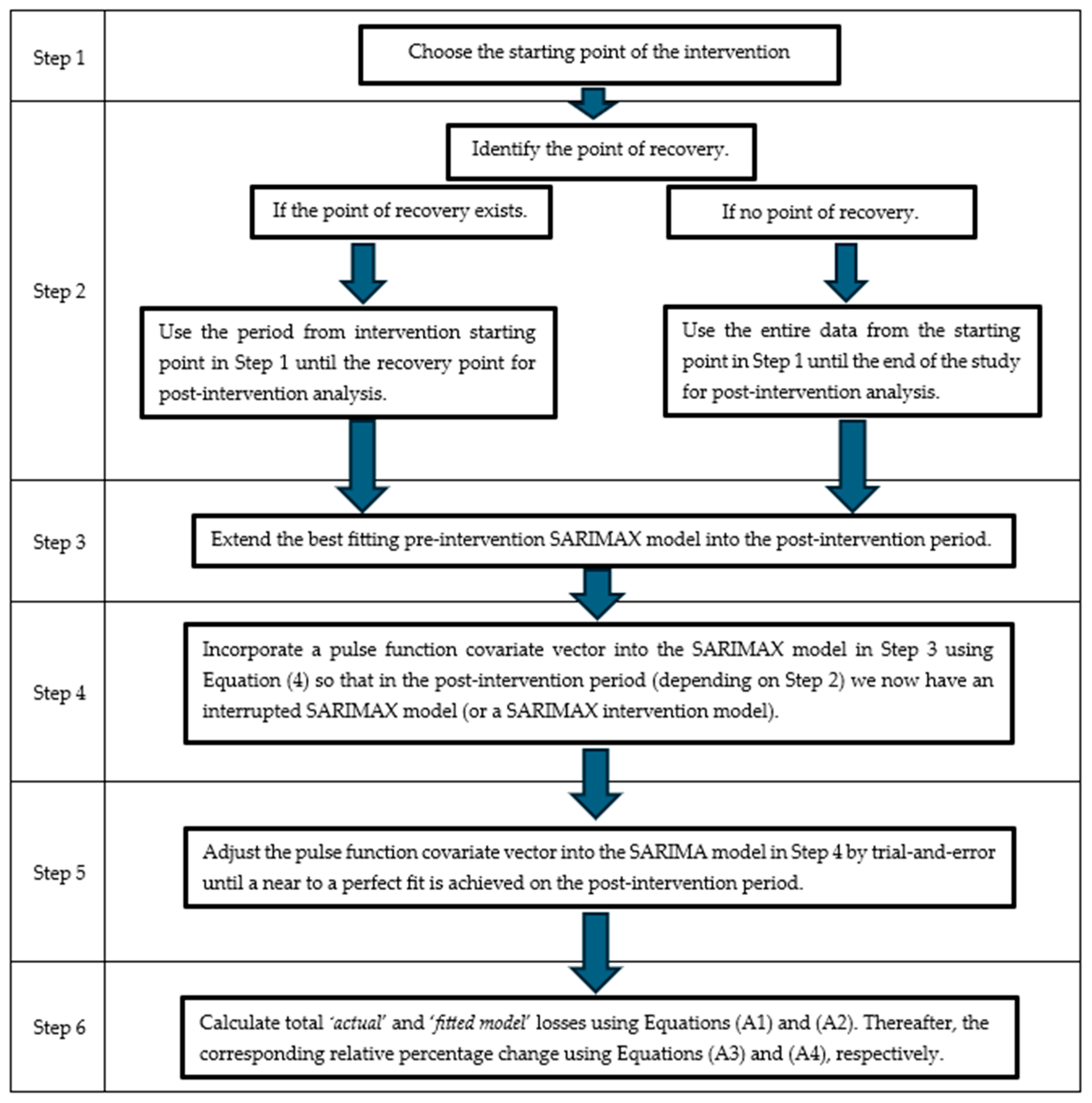
where Y t denotes the total number of interrupted tourist arrivals at t . T k represents the intervention period (for the tourist arrivals dataset considered here, this is 64 months, i.e., from March 2020 to June 2025), P t T k is the intervention indicator variable for a pulse function, ω B = ω 0 ω 1 B ω u B u , and δ ( B ) = 1 δ 1 B δ r B r , where u and r represent the intervention duration and decay pattern, respectively. Other recent studies that have considered the SARIMAX approach include Masena et al. (2024a, 2024b). In this study, we express the pulse function as
P t T k = c o v a r i a t e   v e c t o r ,     i f   t = T k                                                     0 ,     o t h e r w i s e
where a covariate vector is a set of values selected by trial and error using the following steps:
Step 1:
Choose the starting point of the intervention.
Step 2:
Identify the point of recovery.
Step 3:
Extend the best-fitting pre-intervention SARIMA model into the post-intervention period.
Step 4:
Supplement the SARIMA model in Step 3 with the pulse function covariate vector fitted via trial and error to make it a SARIMAX intervention model.
Step 5:
Adjust the components of the pulse function covariate vector one by one starting from the starting point of the intervention in Step 1 to the recovery point or the end of the dataset if there is no recovery point. The aim is to select components of the pulse function covariate vector that produce fitted values that are as close as possible to the actual interrupted series in the post-intervention period. An ideal model will have the lowest mean absolute percentage error (MAPE) and the root mean squared error (RMSE) values (Moreno et al., 2013).
Step 6:
The SARIMAX intervention model in Step 4 and Step 5 is then used to calculate estimated losses in the intervention period.

2.4. Data Preparation and Stationarity

Box–Cox transformation is used to stabilise variation in the series and possibly transform the data such that it closely resembles that of normal distribution (Proietti & Lütkepohl, 2013). It is important to note that data transformation can only be used on a series with positive values and must be conducted prior to applying any differencing on the series. This study applied Box–Cox transformation to ascertain the necessary transformation on A t (Cryer & Chan, 2008) so that, eventually, stationarity of the transformed data can be achieved.
The Augmented Dickey–Fuller (ADF) test was used to assess the null hypothesis that A t is non-stationary, with the alternative hypothesis that A t is stationary being set at a 5% significance level (0.05), meaning that if the p-value is < 0.05 , the null hypothesis will be rejected, and it will be concluded that A t is stationary. Also, the Kwiatkowski–Phillips–Schmidt–Shin (KPSS) test examines the null hypothesis that   A t is trend-stationary, with the alternative hypothesis that A t is not trend-stationary being set at the 5% (0.05) significance level (Su et al., 2012), meaning that if the p-value is > 0.05 , the null hypothesis will not be rejected and it will be concluded that A t is trend-stationary. The test statistics for the ADF and KPSS tests are given as follows:
t δ = δ s . e . δ
where s . e . δ is the standard error of the estimated coefficient δ (Herranz, 2017) and
K P S S = n 2   t = 1 n S ^ t 2 λ ^ 2
where S ^ t = i = 1 t u ^ i , u ^ i represents the residuals of the fitted regression, n is the sample size, and λ ^ 2 is a consistent estimate of the long-term variance for the residuals.
Overall, the Box–Jenkins methodology can be summarised as shown in Figure 1, with Step 0 being discussed in this section and the remaining steps being discussed in the following subsections.

2.5. Model Specification and Accuracy

In the SARIMA model’s specification stage, several time series models are identified and the concrete values of SARIMA p , d , q P , D , Q s are determined from the patterns of the Autocorrelation function (ACF) and the Partial Autocorrelation Function (PACF). The model with the lowest values of the Akaike’s Information Criterion (AIC) and Bayesian Information Criterion (BIC) is deemed the most suitable (Cryer and Chan, 2008). The AIC and BIC values are calculated as
A I C = 2 l o g   L + 2 k       a n d   B I C = 2 l o g ( L ) + k l o g ( n ) ,
where L is the likelihood function of the series, n is the number of observations, and k = p + q .
The prediction accuracy of the selected model is evaluated using the root mean squared error (RMSE) and mean absolute percentage error (MAPE) (Hodson, 2022; Chicco et al., 2021),
R M S E = 1 n t = 1 n A t A ^ t 2   a n d   M A P E = 1 n t = 1 n A t A ^ t A t × 100 ,
where   A t and A ^ t represent the observed and predicted values, respectively.

2.6. Parameter Estimation

The best possible parameter estimates of the selected model are evaluated using maximum likelihood estimation (MLE) as per the log-likelihood function,
ψ ^ n = a r g   m a x ψ Ψ L n Y t ; ψ = a r g   m a x ψ Ψ L n ψ
where ψ ^ n is the n th estimated parameter. Parameter estimates are determined by solving for the derivative of the log-likelihood function. The advantage of using MLE is embodied in the understanding that it is consistent and uses all the information in the data instead of using only the first and second moments, as seen for the least squares method (Cryer and Chan, 2008).

2.7. Model Diagnostics

This current study used the Ljung–Box and Box–Pierce tests to assess the null hypothesis that the standardised residuals from the fitted model are not autocorrelated, with the alternative hypothesis being that the standardised residuals are autocorrelated. Both tests were conducted at the 5% (or 0.05) level of significance. Therefore, the null hypothesis is rejected when the p-values are less than 0.05, and if so, then it is concluded that the standardised residuals are autocorrelated. Also, the normality of the standardised residuals from the selected model was evaluated using the Shapiro–Wilk and Jarque–Bera tests at the 5% significance level. The null hypothesis is that the standardised residuals are normally distributed, and the alternative hypothesis is that the standardised residuals are not normally distributed. If the p-values are less than 0.05, the null hypothesis will be rejected, and if so, then it is concluded that the standardised residuals are not normally distributed (Gujarati & Porter, 2008). The mathematical expressions of the Ljung–Box, Box–Pierce, Shapiro–Wilk, and Jarque–Bera tests are provided in Appendix C.

2.8. R Packages

This study used the R programming software version 4.4.3 with the TSA, forecast, tsoutliers, lmtest, and MASS packages to conduct the analysis—see Cryer and Chan (2008), R Core Team (2025), Hyndman and Khandakar (2008), López-de-Lacalle (2019), Venables and Ripley (2002), and Zeileis and Hothorn (2002).

3. Analysis and Results

3.1. Data Overview

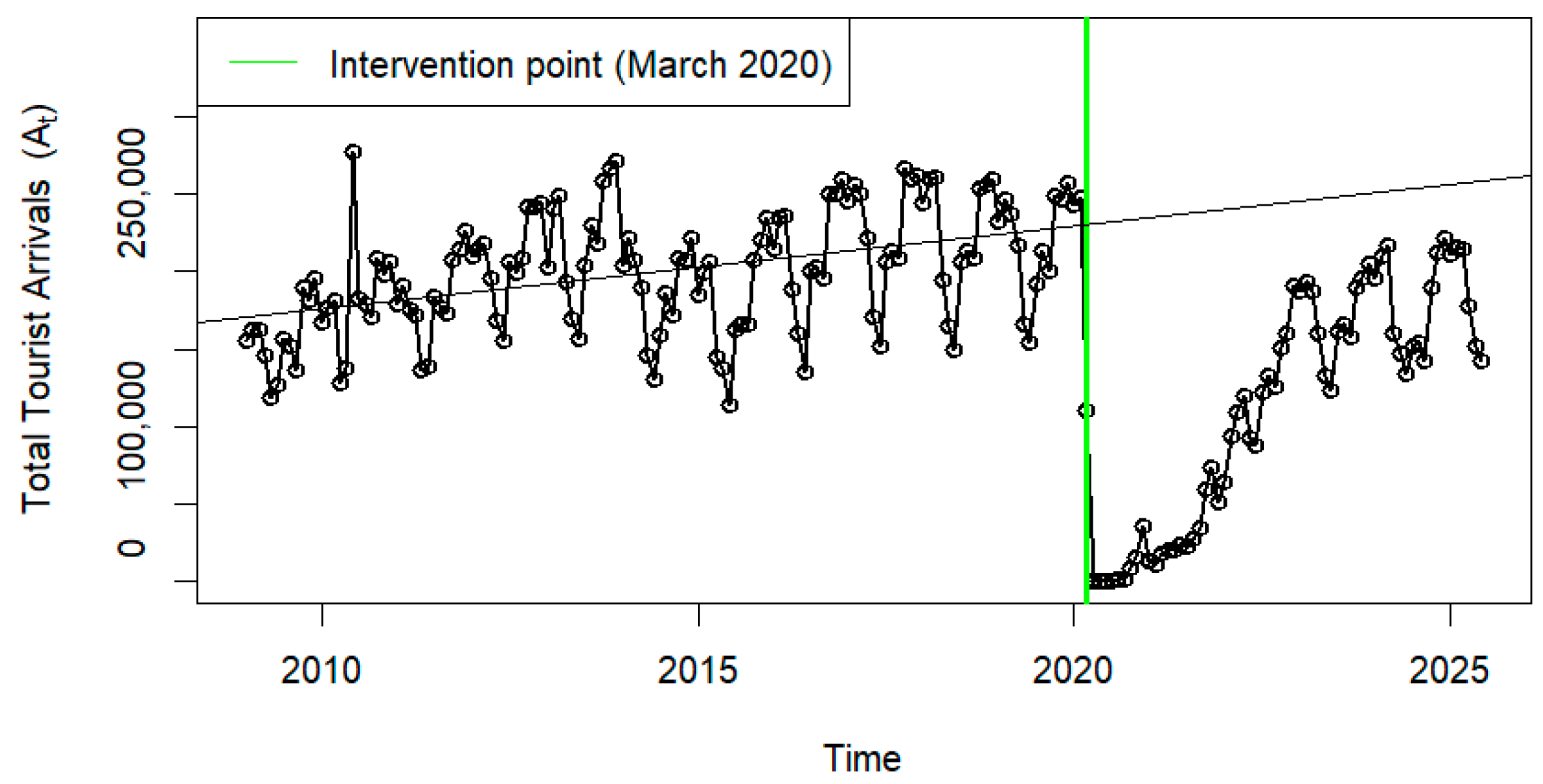
The analysis is based on a dataset detailing the monthly total number of international tourist arrivals into the RSA from January 2009 to June 2025, which can be obtained on Statistics South Africa’s website (https://www.statssa.gov.za, accessed on 27 September 2025) and is included in Appendix A. The pre-intervention period begins in January 2009 and lasts until February 2020 (134 months). March 2020 is the intervention point, and the post-intervention period ranges from March 2020 to June 2025 (64 months). In the time series plot in Figure 2, the tourism arrival series ( A t ) exhibits a highly seasonal behaviour with an overall increasing trend. A sudden significant decline in A t associated with the implementation of a national lockdown is observed in March 2020, where the number of arrivals went from 248,037 in February 2020 to 110,241 in March 2020, and further declined the minimum values of 507 and 315 in April 2020 and May 2020, respectively.

3.2. Pre-Intervention Analysis

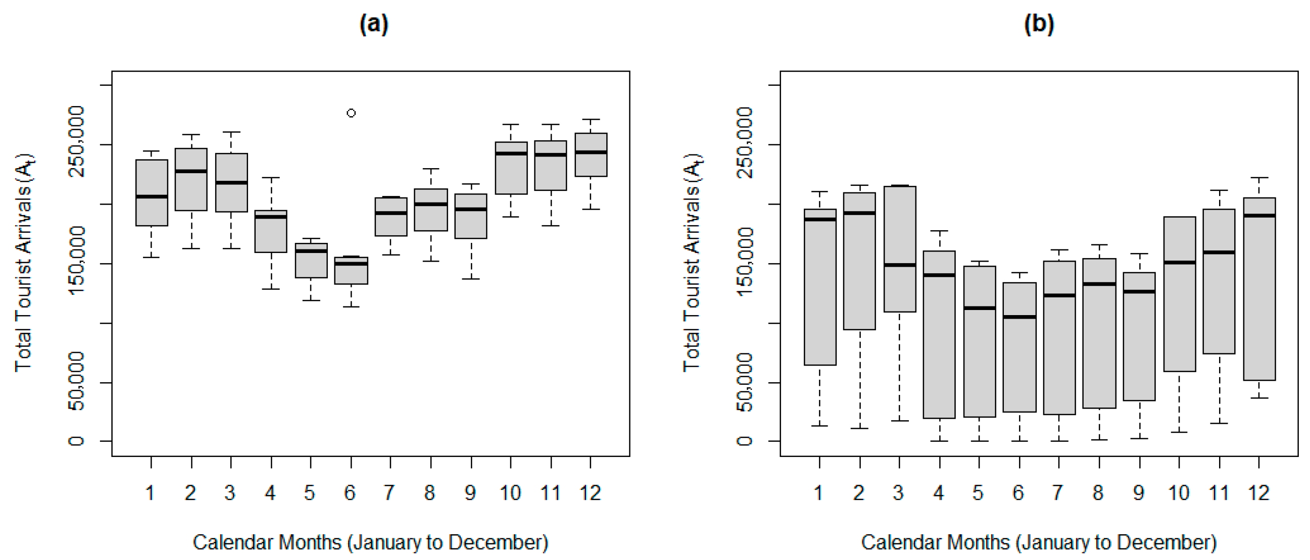
On average, there were 200,484 international tourist arrivals per month into the RSA during the pre-intervention period, with the minimum and maximum being 113,689 and 277,345, respectively. Figure 3a shows that tourist arrivals are generally at their lowest in June (winter) and at their peak between October and December. However, June 2010 is an outlier with the highest number of tourist arrivals due to the FIFA World Cup hosted by the RSA.
In addition, Figure 3b further shows that the minimum, mean, and maximum number of tourist arrivals declined to 315, 114,311 and 222,163, respectively, during the post-intervention period. Overall, a direct comparison of the corresponding monthly boxplots shows that the number of tourist arrivals in South Africa is lower in the post-intervention period as compared to the pre-intervention period.
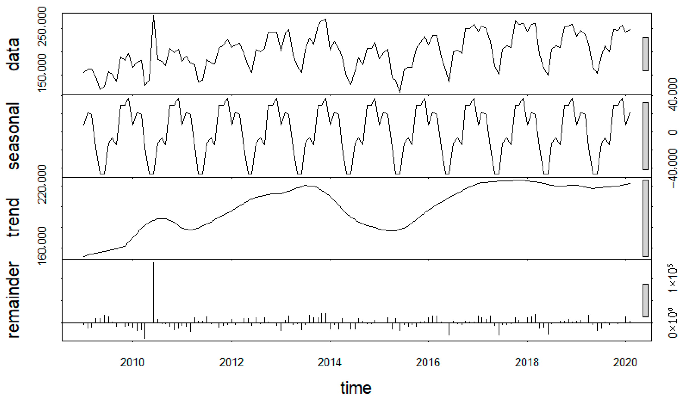
In Figure 4, the original series exhibits random fluctuations, the seasonal component exhibits strong seasonality, and the trend component exhibits gradual cyclical increasing patterns. Generally, the decomposed time series plot in Figure 4 shows a clear increasing trend and seasonality in the number of tourist arrivals. However, in this figure, there is a clear outlier in the remainder plot which corresponds to June 2010. Therefore, first and seasonal differencing of the pre-intervention series are vital to eliminating the trend and accounting for the seasonality within the series. More importantly, the detection of outliers must be implemented.

3.3. Data Transformation

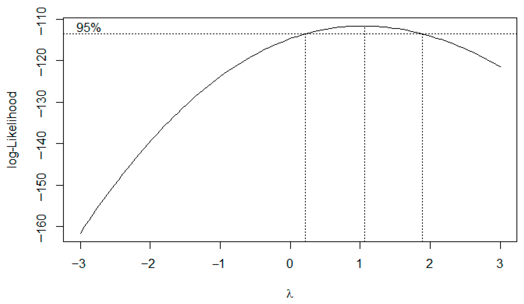
The lambda value from the Box–Cox diagram in Figure 5 is approximately equal to 1 , suggesting that the series ( A t ) does not require any transformation.
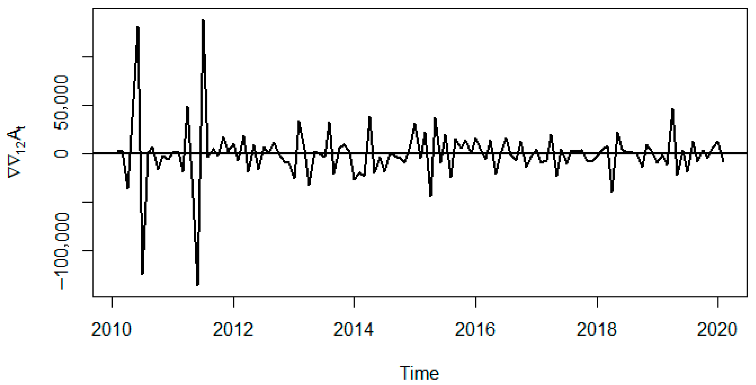
First and seasonally differenced tourist arrivals data ( 12 A t ,   where d = D = 1 and s = 12 ) is depicted in Figure 6, and no noticeable trend is observed. The differenced series seems to be mean reverting, which suggests that 12 A t may be stationary, but we verify this through the ADF test on 12 A t , which produces a statistically significant p-value (0.01) at the 0.05 level of significance. Therefore, the null hypothesis of stochastic non-stationarity is rejected, and thus 12 A t is stochastically stationary. Also, the KPSS test on 12 A t produced a statistically insignificant p-value (0.1) at the 0.05 level of significance, suggesting that the null hypothesis that the series is trend-stationary cannot be rejected; thus, 12 A t is trend-stationary.

3.4. Model Specification

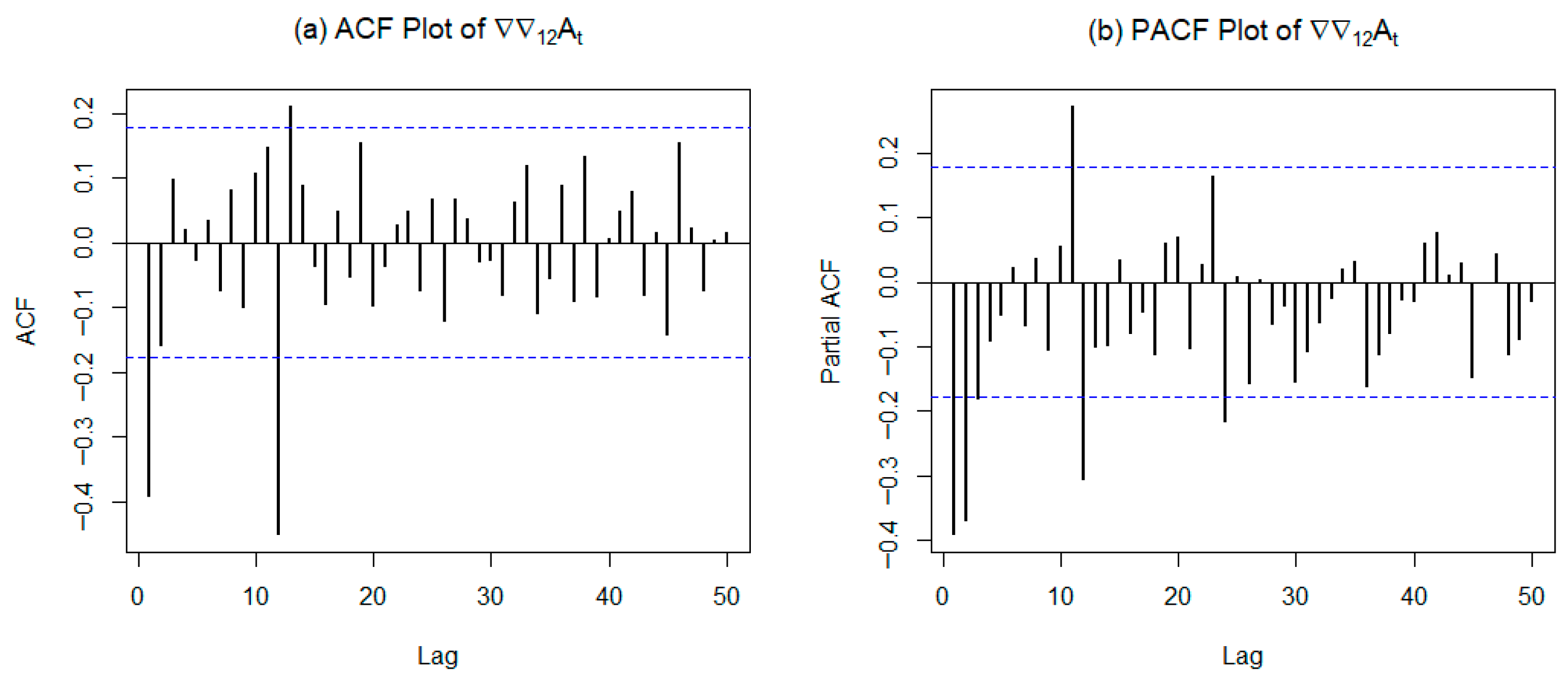
The ACF plot based on the 12 A t presented in Figure 7a has significant lags of 1, 12, and 13. The PACF plot of 12 A t in Figure 7b has significant lags of 1, 2, 11, and 12. Candidate models based on the ACF and PACF in Figure 7a,b are SARIMA 2 , 1 , 2 2 , 1 , 1 12 and SARIMA 2 , 1 , 1 2 , 1 , 1 12 .
Table 1 summarises the AIC, BIC, RMSE, and MAPE values of 10 candidate SARIMA models fitted on the pre-intervention A t utilising the ‘auto.arima’ function in the R forecast package (Hyndman & Khandakar, 2008).
The SARIMA 0 , 1 , 1 0 , 1 , 1 12   model from Table 1 seems to provide the best fit to the RSA tourist arrivals series since it has the lowest AIC and BIC values. However, it does not have the lowest RMSE and MAPE values (but these are very close to the lowest values). The SARIMA 0 , 1 , 1 0 , 1 , 1 12 model is expressed as
1 B 1 B 12 A t = 1 θ 1 B 1 Θ 1 B 12 ε t .
The SARIMA 1 , 1 , 1 0 , 1 , 2 12 seems to be the second-best fitting model due its second lowest AIC and BIC values, as seen in Table 1. Additionally, the RMSE and MAPE values of the SARIMA 1 , 1 , 1 0 , 1 , 2 12 are less than those of the SARIMA 0 , 1 , 1 0 , 1 , 1 12 model. This might suggest that SARIMA 1 , 1 , 1 0 , 1 , 2 12 provides a relatively good fit for the data. The SARIMA 1 , 1 , 1 0 , 1 , 2 12 model is expressed as
1 ϕ 1 B 1 B 1 B 12 A t = 1 θ 1 B 1 Θ 1 B 12 Θ 2 B 24 ε t .

3.5. Parameter Estimation

All parameter estimates in this section were obtained using maximum likelihood estimation (MLE), as described in Section 2.6. The parameters of the SARIMA 0 , 1 , 1 0 , 1 , 1 12 pre-intervention model are provided in Table 2. Both of the model parameters of the SARIMA 0 , 1 , 1 0 , 1 , 1 12 model in Table 2 are statistically significant at the 0.05 level of significance, as indicated by the p-values lower than 0.05.
Outlier detection based on the SARIMA 0 , 1 , 1 0 , 1 , 1 12 model was conducted using the tsouliers R package (López-de-Lacalle, 2019). Two additive outliers were detected in the SARIMA 0 , 1 , 1 0 , 1 , 1 12 model at t = 16 , corresponding to April 2010, and t = 18 , corresponding to June 2010, with statistically significant p-values of 0.001412 and 2.2 × 10⁻¹⁶, respectively, at the 0.05 level of significance. The SARIMA 0 , 1 , 1 0 , 1 , 1 12 model with AO16 and AO18 is expressed as
1 B 1 B 12 A t = 1 θ 1 B 1 Θ 1 B 12 ε t + A O 16 + A O 18 .
Henceforth, the model in Equation (12) will be referred to as SARIMAX 0 , 1 , 1 0 , 1 , 1 12 .
SARIMAX 0 , 1 , 1 0 , 1 , 1 12 has AIC = 2623.04, BIC = 2637.02, RMSE = 10,985.94, and MAPE = 3.99%. The parameters, θ 1 ,   Θ 1 ,   AO16, and AO18 in Table 3 are statistically significant at the 0.05 level of significance. The fitted SARIMAX 0 , 1 , 1 0 , 1 , 1 12 model has lower AIC, BIC, RMSE, and MAPE values compared to SARIMA 0 , 1 , 1 0 , 1 , 1 12 , and thus this model is the best model for the data.
The original SARIMA 0 , 1 , 1 0 , 1 , 1 12 model does not have the lowest RMSE and MAPE values when compared to the other fitted models; thus, it is necessary to also investigate SARIMA 1 , 1 , 1 0 , 1 , 2 12 , since it has the lowest MAPE value and the second lowest values of AIC and BIC. In Table 4, the parameters θ 1 and Θ 1 are statistically significant, whereas ϕ 1 and Θ 2 are statistically insignificant at the 5% significance level. This means that SARIMA 1 , 1 , 1 0 , 1 , 2 12   is not an ideal model for forecasting tourist arrivals.
Outlier detection based on the SARIMA 1 , 1 , 1 0 , 1 , 2 12 model was conducted using the tsouliers R package (López-de-Lacalle, 2019). In this scenario, four additive outliers were identified in SARIMA 1 , 1 , 1 0 , 1 , 2 12 at t = 16 , corresponding to April 2010, t = 18 , corresponding to June 2010, t = 49 , corresponding to January 2013, and t = 76 , corresponding to April 2015 with statistically significant p-values of 1.394 × 10⁻¹⁰, 2.2 × 10⁻¹⁶, 2.117 × 10⁻⁵, and 4.445 × 10⁻⁶, respectively, at the 5% significance level. Additionally, four innovative outliers were identified in SARIMA 1 , 1 , 1 0 , 1 , 2 12 at t = 52 , corresponding to April 2013, t = 56 , corresponding to August 2013, t = 61 , corresponding to January 2014, and t = 112 , corresponding to April 2018, with IO52, IO56, IO61, and IO112 being statistically significant at p-values of 0.0011146, 0.0211197, 0.0005857, and 5.995 × 10 6 , respectively, at the 5% significance level. The SARIMA 1 , 1 , 1 0 , 1 , 2 12 model with additive and innovative outliers is expressed as
1 ϕ 1 B 1 B 1 B 12 A t = 1 θ 1 B 1 Θ 1 B 12 Θ 2 B 24 ( ε t + I O 52 + I O 56 + I O 61 + I O 112 ) + A O 16 + A O 18 + A O 49 + A O 76 .
All parameters of the SARIMAX 1 , 1 , 1 0 , 1 , 2 12 model in Table 5 are statistically significant at the 0.05 level of significance, except for Θ 2 . The SARIMAX 1 , 1 , 1 0 , 1 , 2 12 model has AIC =   2582 .41, BIC =   2618.75 , RMSE =   8724.677 , and MAPE =   3.36 % , which are significantly lower compared to those of the SARIMA 0 , 1 , 1 0 , 1 , 1 12 , SARIMAX 0 , 1 , 1 0 , 1 , 1 12 , and SARIMA 1 , 1 , 1 0 , 1 , 2 12 models. Thus, the SARIMAX 1 , 1 , 1 0 , 1 , 2 12 model is the best fitting model for the pre-intervention period of RSA tourist arrivals and is ideal for forecasting.

3.6. Residual Analysis

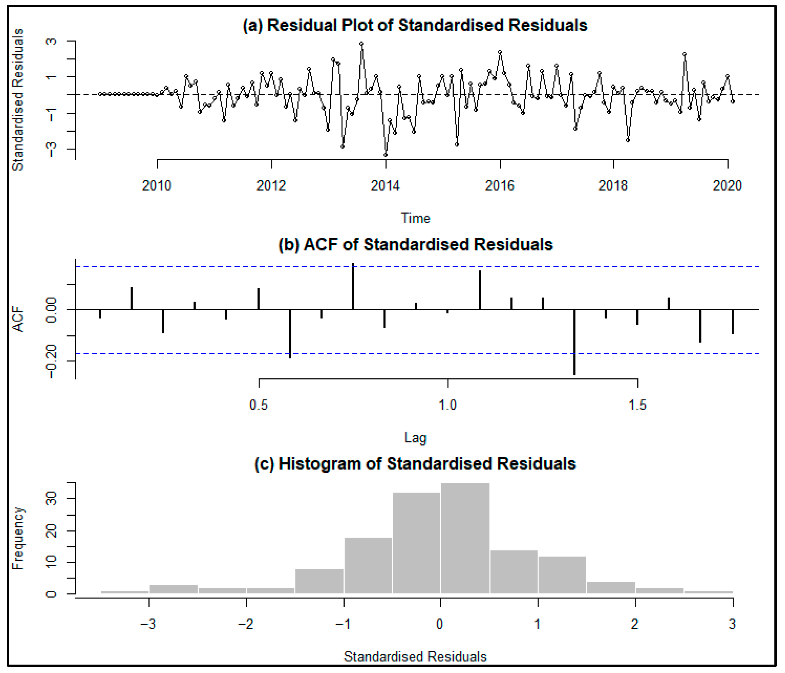
In Figure 8, diagnostic analysis on the residuals of SARIMA 0 , 1 , 1 0 , 1 , 1 12 is conducted. It is evident from the residual plot in Figure 8a that the standardised residuals do not show any structured patterns. The ACF plot in Figure 8b has only three significant lags. Two autocorrelation tests, namely the Ljung–Box (0.2253) and Box–Pierce (0.2836) tests, have p-values greater than 0.05, which means that the null hypothesis (standardised residuals are uncorrelated) is not rejected. This solidifies the null hypothesis that the standardised residuals of the selected SARIMAX 0 , 1 , 1 0 , 1 , 1 12 are not correlated. This shows that the three significant lags in the ACF plot in Figure 8b resulted from random sampling error. The histogram in Figure 8c seems to have a symmetrical shape, but the results of the Shapiro–Wilk (0.002355), and Jarque–Bera (0.001031) tests have p-values that are less than 0.05, which means that the null hypothesis (standardised residuals follow a normal distribution) is rejected. Thus, the standardised residuals from the fitted SARIMAX 0 , 1 , 1 0 , 1 , 1 12 model do not follow a normal distribution. It is evident from these tests that the model assumption of normality is violated. Therefore, it follows that the fitted SARIMAX 0 , 1 , 1 0 , 1 , 1 12 model may not be appropriate for forecasting.
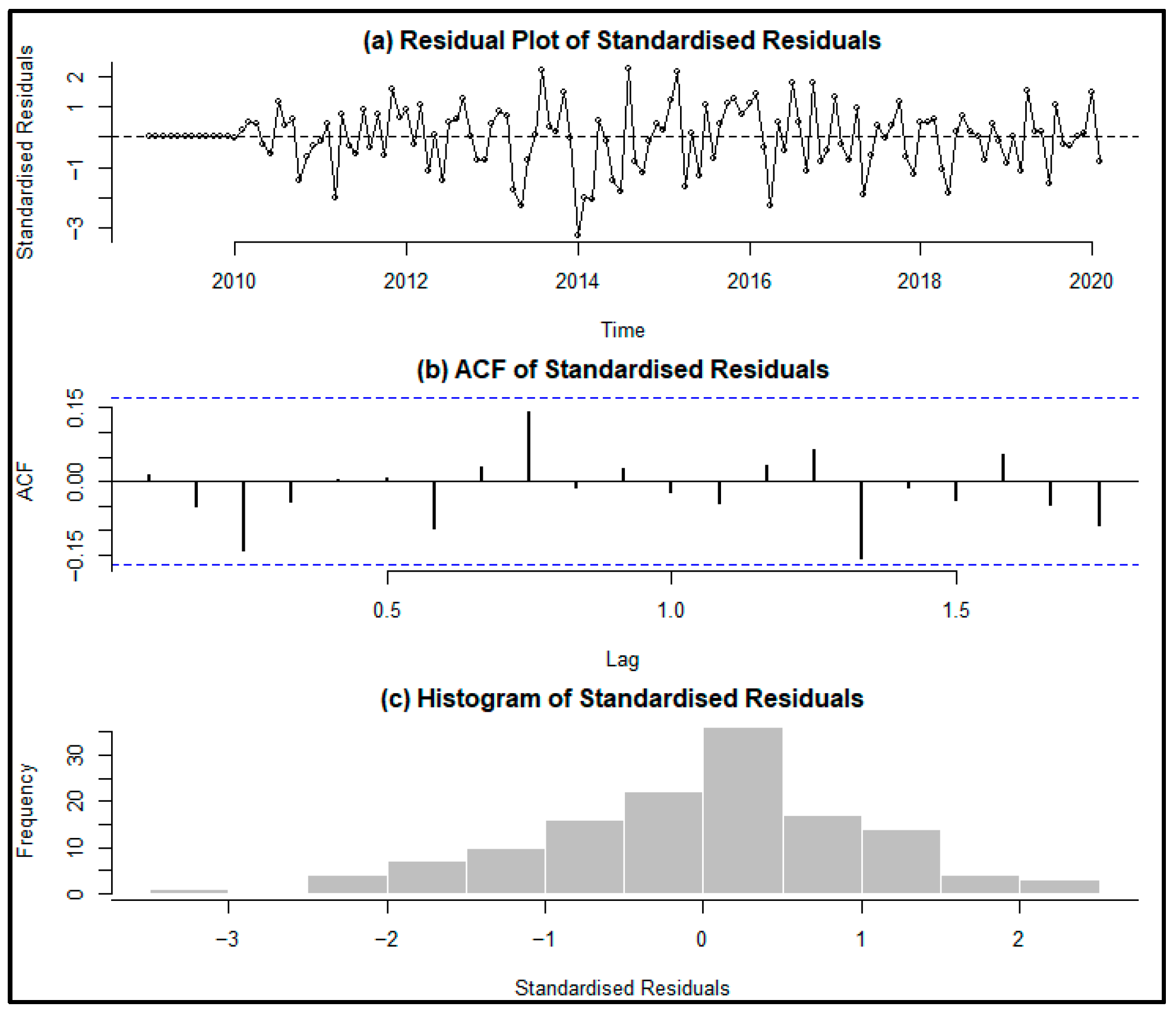
The standardised residuals in Figure 9a do not show any structured patterns, and while the January 2014 point seems suspect, none of the points are outliers. The ACF plot depicted in Figure 9b does not have any significant lags, which suggests that the standardised residuals of the SARIMAX 1 , 1 , 1 0 , 1 , 2 12 model are not autocorrelated. The p-values from the Ljung–Box (0.5053) and Box–Pierce (0.5569) tests are statistically insignificant at the 0.05 level of significance. This solidifies the null hypothesis that the standardised residuals of the selected SARIMAX 1 , 1 , 1 0 , 1 , 2 12 model are uncorrelated. The histogram in Figure 9c slightly mimics that of a normal distribution. The p-values from the Shapiro–Wilk (0.126) and Jarque–Bera (0.2106) tests are statistically insignificant at the 0.05 level of significance. Thus, the standardised residuals for the SARIMAX 1 , 1 , 1 0 , 1 , 2 12 model do not violate the model assumption of normality. Hence, it is concluded that the standardised residuals from the fitted SARIMAX 1 , 1 , 1 0 , 1 , 2 12 model are white noise.

3.7. Actual Data in Comparison with Fitted Values

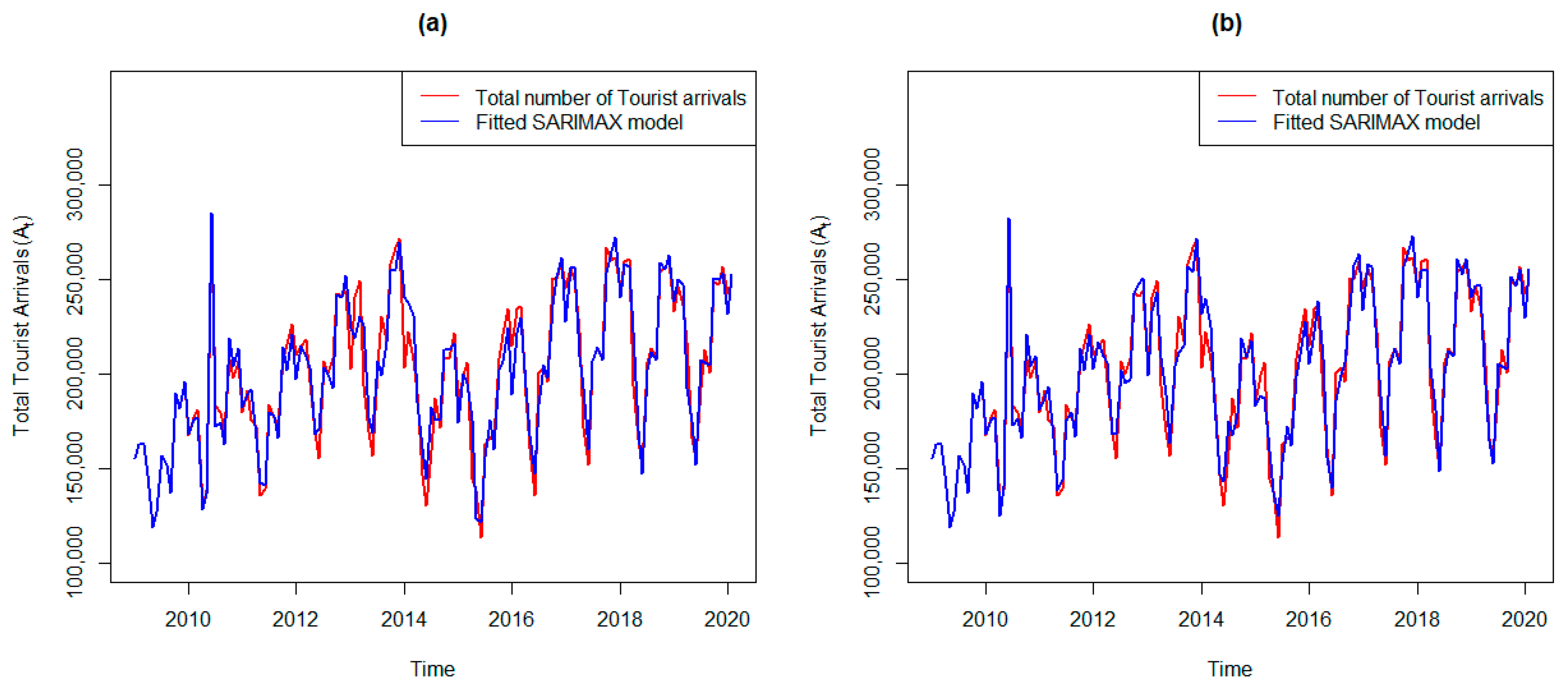
Figure 10a,b presents the time series plot comparing the actual A t and fitted values ( A ^ t ) of tourist arrivals into the RSA for both SARIMAX 0 , 1 , 1 0 , 1 , 1 12 and SARIMAX 1 , 1 , 1 0 , 1 , 2 12 , respectively. During the pre-intervention period, the fitted values of both models are not significantly different from the actual values. However, SARIMAX 1 , 1 , 1 0 , 1 , 2 12 is an ideal model for forecasting RSA tourist arrivals because it has the best fit on the pre-intervention ( A t ) data and it also follows white noise processes, as shown in Section 3.5 and Section 3.6, respectively.

3.8. Forecasting

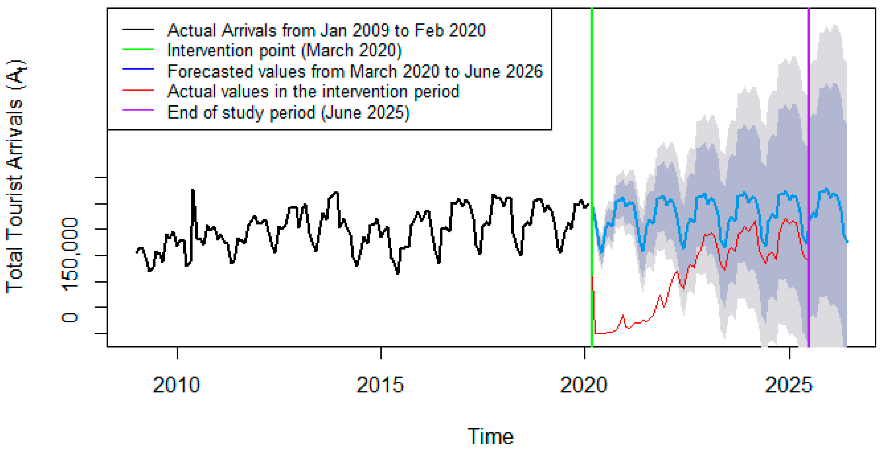
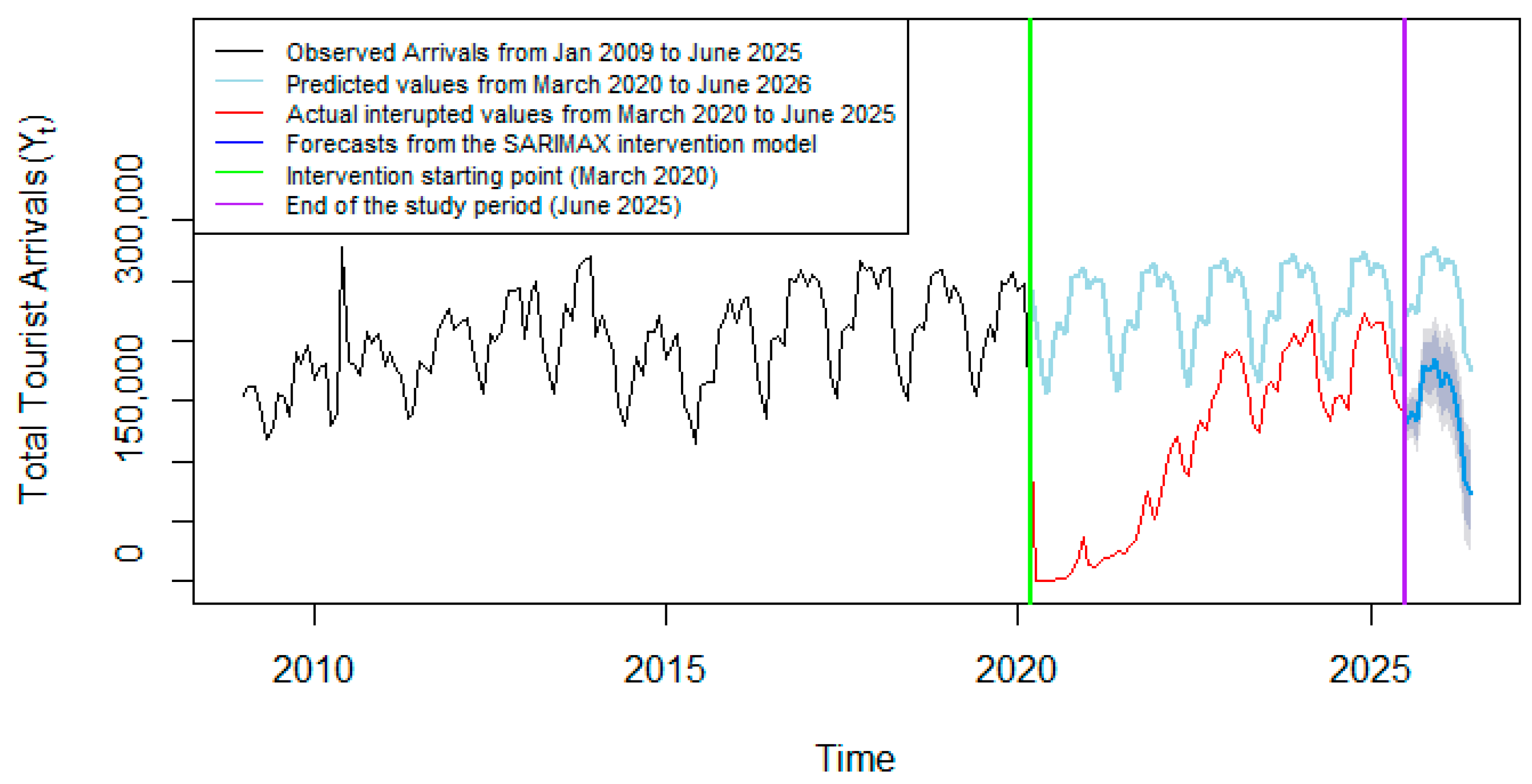
In Figure 11, the actual values of A t before the intervention are represented by the black series. March 2020 marks the intervention’s starting point, indicated by the green vertical line. The red line indicates the interrupted actual values of A t from March 2020 to June 2025. The blue line depicts the in-sample forecasts generated by the SARIMAX 1 , 1 , 1 0 , 1 , 2 12 model for March 2020 to June 2025, as well as 1-year out-of-sample forecasts starting at July 2025 and lasting until June 2026. The gap/area between the observed tourist arrivals (red line) and forecasted arrivals (blue line) from March 2020 started to reduce over time, but tourist arrivals failed to recover to their pre-intervention levels. This reveals that the COVID-19 pandemic continues to have a long-lasting negative and undesirable impact on RSA tourist arrivals. The light grey shading represents the 95% confidence limits, whereas the dark grey shading represents the 80% confidence limits. The prediction limits in Figure 11 are narrow at the beginning of the in-sample forecasts but become wider over time due to increased uncertainty. The out-of-sample forecasts also imitate the stochastic periodicity depicted by the series before the intervention occurred. Given that the interrupted series did not bounce back to its pre-intervention level, intervention analysis in the next section will be conducted based on the 64-month post-intervention period.

3.9. Post-Intervention Analysis

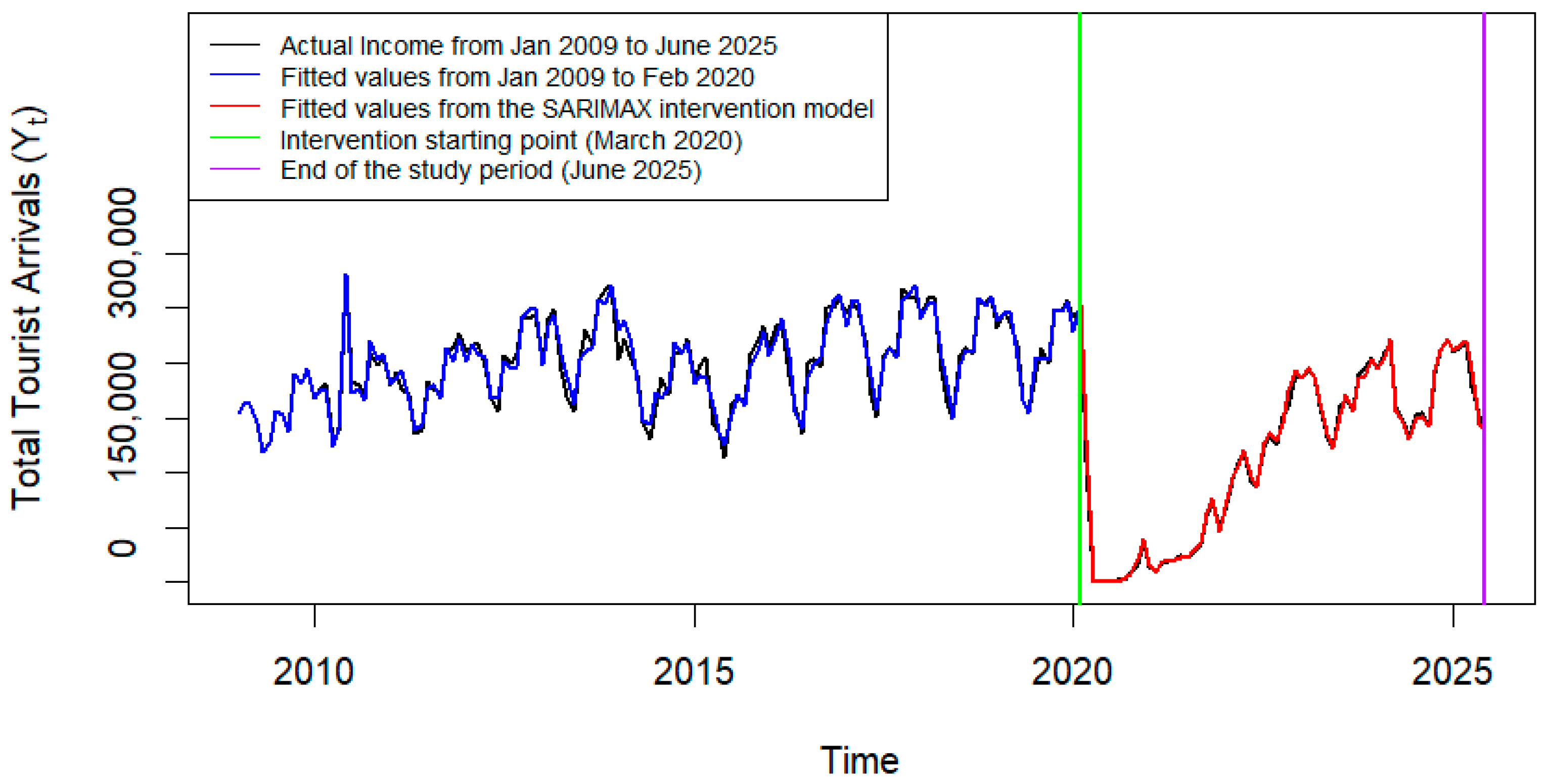
In this section, the SARIMAX 1 , 1 , 1 0 , 1 , 2 12 model based on A t before the intervention is expanded into the 64-month post-intervention period and augmented with a pulse function covariate regression vector as an exogenous component through trial and error. The resulting model becomes a SARIMAX 1 , 1 , 1 0 , 1 , 2 12 intervention model, which will be referred to as the “SARIMAX intervention model” from here onwards. The fitted values of the SARIMAX intervention model in Figure 12 produced an excellent fit on the actual interrupted Y t during the post-intervention period, and thus the model is a good fit. Therefore, the fitted SARIMAX intervention model is used to quantify intervention effects in Section 3.10. The fitted SARIMAX intervention model has an RMSE value of 4865.5 and an MAPE value of 9.25%. The MAPE value of 9.25% implies that Y ^ t differs by 9.25% on average in comparison with Y t . Thus, the model is appropriate for capturing and quantifying the impact of the COVID-19 pandemic and the response to it on Y t .

3.10. Quantification of Pandemic Effects

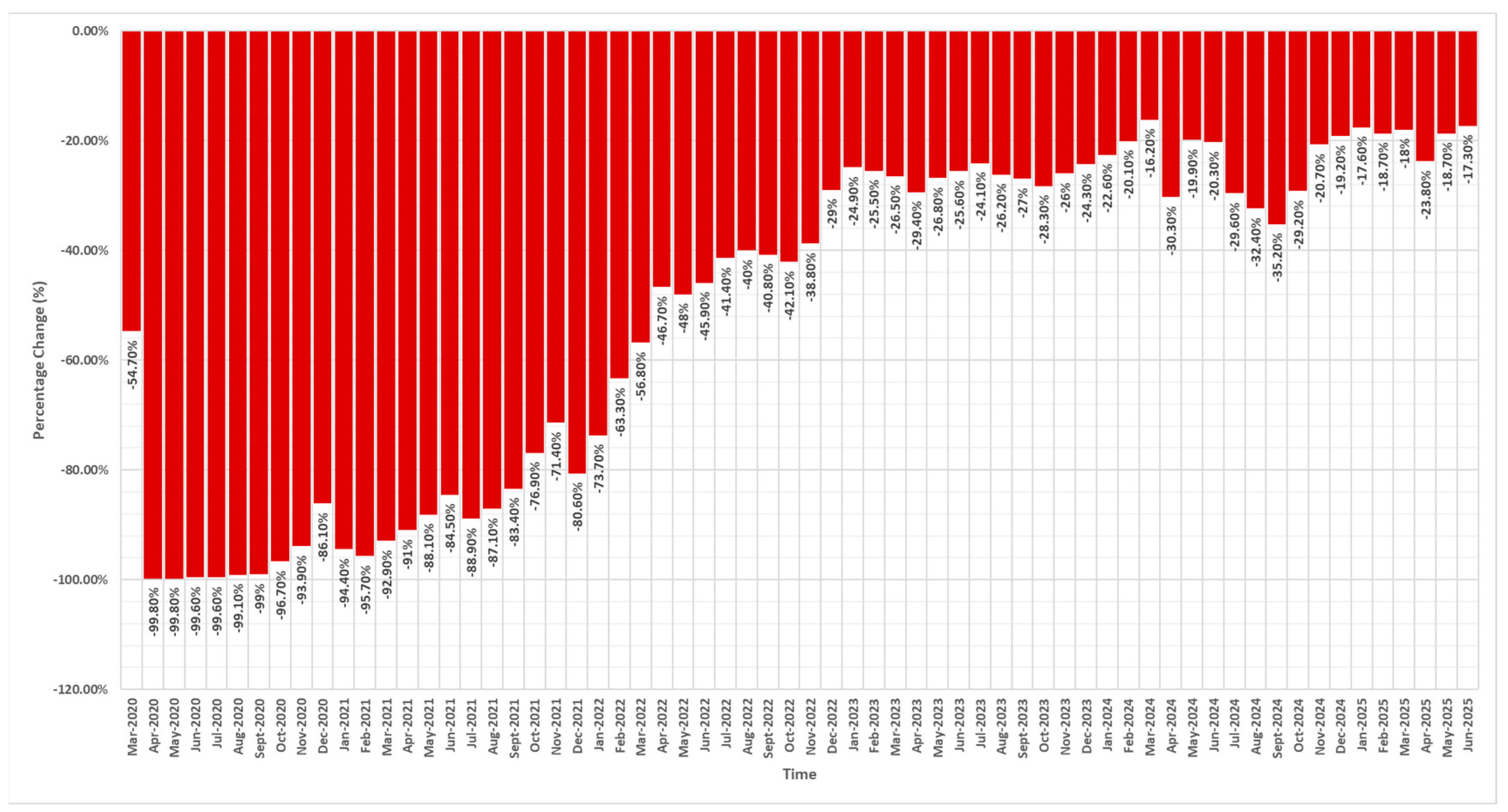
Technical computations of the quantification of the COVID-19 pandemic’s effects are provided in Appendix B. In March 2020, just after the announcement of lockdown level 5, the number of tourist arrivals dropped to 110,241, which correspond to a 54.70% reduction (shown numerically in Appendix B and graphically in Figure 13). The number of tourist arrivals was severely affected in May 2020, dropping to 315, which is a significantly lower value compared to other months during the post-intervention period. This corresponds to a 99.8% reduction in expected tourist arrivals when compared to 171,169 as predicted by the pre-intervention SARIMAX model. This means that the number of tourist arrivals in May 2020 was approximately 99.8% (170,854) lower than it would have been in the absence of the COVID-19 pandemic. The value for June 2025 corresponds to a reduction of −17.3% (29,816), which shows that COVID-19 is still negatively affecting the number of international tourist arrivals as of the end of the study period.
Overall, Figure 13 highlights that international tourist arrivals drastically dropped in March and April 2020 as a result of the strict level 5 lockdown. In May 2020, the RSA government adjusted the lockdown to level 4, but the percentage difference between the pre-intervention forecast and the actual values is at a high value of 99.80%, irrespective of the adjustment in level. From 1 June 2020 to 17 August 2020, the RSA adjusted to lockdown level 3, and the number of tourist arrivals increased by only 0.40%. During the period between 18th August and 28th December, lockdown levels 2 and 1 were implemented and the percentage difference between the pre-intervention forecast and the actual values for tourist arrivals improved. From July 2021 to June 2025, this percentage difference continued to decrease to around 17.30%, but the total number of tourist arrivals did not fully bounce back to its pre-intervention level, since the percentage change (lingering effect) remains negative.
The 1-year out-of-sample forecasts produced by the SARIMAX intervention model in Figure 14 suggest that, with all other factors kept constant, the number of tourist arrivals in the RSA’s tourism sector will not return to its pre-intervention baseline by June 2026.

4. Discussion of Research Questions

This study noted multiple inconsistencies in the three publications that conducted time series analysis on the exact RSA tourist arrivals data used here. Firstly, the descriptive statistics in Chipumuro et al. (2024a) differ significantly from those in Chipumuro et al. (2024b) for the same data ranging from January 2009 to December 2023. Secondly, both studies by Chipumuro et al. (2024a, 2024b) used RSA tourist arrivals data ranging from January 2009 to February 2019 to perform pre-intervention modelling; however, Chipumuro et al. (2024a) did not conduct any data transformation in the pre-intervention series and concluded that ARIMA 1 , 0 , 1 0 , 1 , 1 12 with drift is the most suitable model, whereas Chipumuro et al. (2024b) used square root transformation and selected the ARIMA 0 , 1 , 1 0 , 1 , 1 12 model as the best-fitting model. Also, Chipumuro and Chikobvu (2022) developed the pre-intervention model using data from January 2009 to August 2019 with a log transformation and selected ARIMA 1 , 0 , 0 1 , 0 , 0 12 as the best fitting model. Note, however, that our current study uses data from January 2009 to February 2020 without any transformation (due to the deduction from the Box–Cox transformation in Figure 5 here) as the pre-intervention period and March 2020 as the intervention point, backed by the implementation of level 5 lockdown by the RSA government towards the end of March 2020. Thirdly, the residual plots of fitted models (including when inspecting the decomposition plots) in all three studies (i.e., Chipumuro & Chikobvu, 2022; Chipumuro et al., 2024a, 2024b) clearly indicate the presence of multiple outliers, including June 2010 during the FIFA World Cup, yet none of these studies conducted outlier detection in order to incorporate these outliers into the building of the pre-intervention model and improve the accuracy of the fitted model. On the contrary, the current study conducted outlier detection and incorporated eight outliers (i.e., four innovative and four additive) into the best fitting SARIMA pre-intervention model. The residual plot in Figure 9a clearly shows that the chosen model captures the effect of all outliers well. Consequently, to address RQ1, it follows that SARIMAX is a better model for implementation in this scenario than the SARIMA model.
Fourthly, in Chipumuro et al. (2024a, 2024b), the authors asserted that the plot of actual values versus forecasted values in the validation period provides enough evidence that the fitted pre-intervention models had good forecasting power. This is misleading as error metrices such as MAPE and RMSE were not used to cement this assertion. Thus, the analysis conducted in this current study reveals that incorporating a pulse function covariate vector through trial and error can produce a suitable model with fitted values that are very close to the actual interrupted values with a relatively low MAPE value. It is worth mentioning that Chipumuro and Chikobvu (2022) and Chipumuro et al. (2024a, 2024b) did not explicitly provide estimates of total loss in tourist arrivals because of the COVID-19 pandemic. The fitted SARIMAX intervention model in this study successfully estimated the loss of total tourist arrivals from March 2020 to June 2025 as 7,328,919. This estimate deviates from the observed loss of tourist arrivals calculated using actual values by merely 0.62%. This addresses RQ2 by providing the estimated total losses in the number of tourist arrivals into the RSA. These results show the prowess of the SARIMAX intervention model in quantifying the impact of the COVID-19 pandemic over the traditional SARIMA models, and more importantly, in both Figure 11 and Figure 13, it is shown that the tourist arrivals series has not recovered to its pre-COVID-19 levels (which addresses RQ3). Finally, RQ4 is addressed by Figure 14, where it is illustrated (through the 1-year or 12-month forecast using the SARIMAX model) that the number of tourist arrivals will not have recovered by June 2026.

5. Conclusions

This study concludes that the COVID-19 pandemic had an immediate, negative, and continually lingering impact on the total monthly international tourist (headcount) arrivals into the RSA from March 2020 to June 2025. In the pre-intervention modelling, four additive outliers and innovative outliers were detected and incorporated into the SARIMA 1 , 1 , 1 0 , 1 , 2 12 model. Therefore, the SARIMAX 1 , 1 , 1 0 , 1 , 2 12 model is selected as the most appropriate fitting pre-intervention model according to model evaluation metrics. Furthermore, SARIMAX 1 , 1 , 1 0 , 1 , 2 12 passed all model diagnostic tests of the Box–Jenkins methodology because its standardised residuals are random, uncorrelated, and normally distributed. Moreover, its in-sample and out-of-sample forecasts imitate the stochastic periodicity (trend and seasonality components) of the data in the period before the intervention. In the post-intervention period, the SARIMAX 1 , 1 , 1 0 , 1 , 2 12 model is incorporated with the pulse function covariate vector through trial and error and successfully captures the negative effect of the COVID-19 pandemic. March 2020 served as the intervention point, with 133,142 arrivals being recorded in this month, representing 54.70% of the estimated value of 243,383 arrivals had there been no COVID-19 pandemic. May 2020 is the worst affected month in the post-intervention period, as it had merely 315 arrivals compared to the estimated/predicted value of 171,169 arrivals (a 99.80% reduction) had there been no COVID-19 pandemic. More importantly, June 2025 recorded 29,816 (or 17.30%) fewer tourist arrivals than the predicted value of 171,884 (had there been no COVID-19 pandemic), which shows that COVID-19 continues to negatively affect the RSA’s international tourist arrivals, i.e., the lingering effect is still ongoing. Therefore, the total estimated losses in the 64 months of the post-intervention period (March 2020 to June 2025) amounted to 7,328,919.
For future work, researchers can use the Vector AutoRegressive (VAR) and the multivariate SARIMAX models to simultaneously study the relationship between the RSA’s tourist arrivals and tourist accommodation income datasets amidst the COVID-19 pandemic. Other researchers can also conduct a cross-sectional study using tourist arrivals datasets from multiple African countries using exponential smoothing (ETS), hierarchical forecasting, and other machine learning and hybrid models, as seen in Kourentzes et al. (2021) and Qiu et al. (2021). A comparative study between the SARIMAX intervention model used in this study and non-linear models (such as the regime switching and threshold autoregressive models) could be adopted to investigate which model(s) can most accurately and efficiently quantify the impact of COVID-19 on the RSA’s tourist arrivals. This current study conducted research from a time series (or statistical) perspective; however, this can be approached from a different economic perspective by linking it to ‘tourism resilience frameworks recovery modelling theory’ and further link forecasting to policy and strategic recovery decisions, as well as considering structural breaks. In this research work, the forecast discussion does not explain what sectors (e.g., hospitality, flights, small-scale tourism enterprises) were most impacted in the RSA; thus, for future research, this could be a valuable direction to investigate.

6. Limitations of the Study

The SARIMAX intervention model is subject to practitioner–practitioner variation, as various researchers may use different values when performing trial and error. Although the SARIMAX intervention model is suitable for approximating the impact of COVID-19 on tourist arrivals, the use of the trial and error technique is time-consuming and may not be efficient for use in interrupted time series studies with larger post-intervention periods. This model relies heavily on the accurate identification of the timing and nature of interventions, a process that often depends on subjective trial and error procedures. This reliance introduces the potential for researcher bias, data-snooping risks, and inconsistencies in model specification, particularly when contextual information is incomplete or ambiguous. Errors in specifying the underlying ARIMA structure or seasonal components can propagate through the intervention terms, leading to distorted parameter estimates. The approach also requires high-quality, regularly spaced data; missing observations or unmodelled structural breaks can undermine the stability and reliability of results. Additionally, when numerous interventions or long seasonal cycles are incorporated, the estimation process can become computationally burdensome, particularly in large datasets, making the model less scalable compared with more adaptive techniques such as machine learning or state-space approaches.

Author Contributions

Conceptualization, A.M.M., S.C.S., T.E.M. and F.F.K.; methodology, A.M.M.; software, A.M.M.; validation, S.C.S., T.E.M. and F.F.K.; formal analysis, A.M.M.; investigation, A.M.M.; resources, S.C.S., T.E.M. and F.F.K.; data curation, A.M.M.; writing—original draft preparation, A.M.M.; writing—review and editing, S.C.S., T.E.M. and F.F.K.; visualisation, A.M.M.; supervision, S.C.S., T.E.M. and F.F.K.; project administration, S.C.S.; funding acquisition, F.F.K. All authors have read and agreed to the published version of the manuscript.

Funding

This research received no external funding. The APC was funded by the UFS’ Actuarial Development Programme.

Data Availability Statement

The data used in this study is provided in Appendix A.

Conflicts of Interest

The authors declare no conflicts of interest.

Abbreviations

The following abbreviations are used in this manuscript:
ACFAutocorrelation Function
AICAkaike’s Information Criterion
AOAdditive Outlier
ARIMAAutoregressive Integrated Moving Average
BICBayesian Information Criterion
IOInnovative Outlier
MAPEMean Absolute Percentage Error
PACFPartial Autocorrelation Function
RMSERoot Mean Squared Error
RSARepublic of South Africa
SARIMASeasonal Autoregressive Integrated Moving Average
SARIMAXSeasonal Autoregressive Integrated Moving Average with exogenous variables

Appendix A. Dataset

Table A1. Number of tourist arrivals from January 2009 to June 2025.
JanuaryFebruaryMarchAprilMayJuneJulyAugustSeptemberOctoberNovemberDecember
2009155,228162,714162,562146,504118,718126,857156,846152,187136,767189,932181,923195,739
2010167,706177,165181,125128,773138,261277,345183,042179,658171,158208,276197,930206,555
2011179,493190,865175,876172,145135,922139,063183,426176,696173,497208,141215,235226,360
2012210,254214,594218,436195,934168,796155,464206,656199,820208,203242,475241,413243,718
2013202,548240,387249,009193,848169,376156,563204,120230,374217,645258,380266,946271,435
2014203,604221,945207,093189,943146,342130,410159,368186,801171,791208,263207,801221,348
2015184,864199,029205,909144,771138,258113,689162,733165,990166,053208,020221,149234,523
2016214,903234,707235,640188,491160,627135,780200,901203,421196,098250,737250,017259,724
2017245,074255,901249,641222,055171,417151,736206,737213,294208,720267,025259,805261,728
2018244,657259,123260,514194,017165,137149,791206,076213,761209,185253,945256,537259,403
2019232,872246,394236,647217,131166,227154,361192,277213,074200,571248,673247,136256,796
2020242,550248,037110,24150731554987319502084832515,52036,357
202113,68710,74517,54819,91520,76224,54822,87728,15734,89559,47573,67951,516
202264,71493,899108,974119,51892,36887,685122,720132,757126,409151,189159,771190,667
2023187,189192,835187,631160,647132,443123,069161,376165,705158,407189,778195,549205,684
2024195,423209,545216,563160,708147,428134,396152,082153,913142,510189,575212,335222,163
2025210,709215,830214,546178,195152,398142,068

Appendix B. Quantification of COVID-19 Pandemic’s Lingering Effect
The total actual losses in the post-intervention period in Equation (A1) are calculated taking the sum of each monthly differences between the actual values (denoted as A c t u a l   v a l u e t or A t ) and predicted values from the pre-intervention model had there been no intervention in the process (denoted as P r e d i c t e d   v a l u e t or A ^ t ):
i = 1 n ( A c t u a l   v a l u e t P r e d i c t e d   v a l u e t ) = i = 1 n ( A t A ^ t ) .
Next, the total approximated losses in the post-intervention period in Equation (A2) are based on the sum of each monthly difference between the fitted values using the SARIMAX model (denoted as F i t t e d   v a l u e t or A ˇ t ) and predicted values from the pre-intervention model had there been no intervention in the process (denoted as P r e d i c t e d   v a l u e t or A ^ t ):
i = 1 n ( F i t t e d   v a l u e t P r e d i c t e d   v a l u e t ) = i = 1 n ( A ˇ t A ^ t ) .
Finally, to calculate the percentage deviation for each of the months within Equations (A1) and (A2), the relative percentage change (RPC) between the actual values ( R P C A c t u a l ) and fitted values ( R P C F i t t e d ) are computed as follows:
R P C A c t u a l = A t A ^ t A ^ t × 100 %
R P C F i t t e d = A ˇ t A ^ t A ^ t × 100 % .
To visualise the post-intervention flow of the process outlined above, Figure A1 is constructed.
Table A2 reports the approximated effects of the COVID-19 pandemic on the tourist arrivals for each month in the post-intervention period (i.e., March 2020 to June 2020) via the utilisation of Equations (A1) to (A4). For instance, in April 2020, had there been no pandemic, the estimated (or forecasted) number of tourist arrivals would have been 217,562 according to the model fitted on the pre-intervention period. However, due to the declaration of the COVID-19 pandemic in March 2020, there was an abrupt drop at the start of this month. The most noticeably negatively affected month was April 2020, which experienced the largest drop in the number of international tourist arrivals, with the actual loss and fitted model loss values equal to −217,055 and −216,767, respectively, representing a percentage drop of 99.80% and 99.60% for the actual and fitted model loss, respectively. Overall, in Table A2, it follows that the total actual loss of tourist arrivals during the post-intervention period amount to 7,328,919. Similarly, the total fitted model losses amount to 7,283,540 when using the SARIMAX intervention model. Comparing these two values indicates that the SARIMAX intervention model has an approximate difference of 0.62% (or 45,379 fewer tourist arrivals) as compared to the actual number of tourist arrivals. This serves as evidence that the chosen SARIMAX intervention model adequately captured the impact of the COVID-19 pandemic on the total number of arrivals in the post-intervention period and is ideal for forecasting future tourist arrivals, as in general, the percentage values produced by (A4) are actually very close to the actual or observed ones in (A3).
Figure A1. Flowchart for the post-intervention quantification of a lingering effect in a time series due to an intervention.
Economies 13 00362 g0a1
Table A2. Estimated effects of the COVID-19 pandemic on Y t in the post-intervention period.
Actual vs. Predicted ValuesFitted vs. Predicted Values
Postintervention PeriodPredicted Values per Month, A ^ t Actual Values per Month, A t Actual Losses per Month,
( A t A ^ t )
% Change, R P C A c t u a l Covariate VectorFitted Values per Month, A ˇ t Estimated Losses per Month,
( A ˇ t A ^ t )
% Change, R P C F i t t e d
Mar-2020243,383110,241−133,142−54.70%0.95130,061−113,322−46.60%
Apr-2020217,562507−217,055−99.80%1.7795−216,767−99.60%
May-2020171,169315−170,854−99.80%1.3140−171,029−99.90%
Jun-2020155,996549−155,447−99.60%1.2258−155,738−99.80%
Jul-2020200,858873−199,985−99.60%1.55508−200,350−99.70%
Aug-2020214,7021950−212,752−99.10%1.68705−213,997−99.70%
Sept-2020206,0762084−203,992−99%1.583460−202,616−98.30%
Oct-2020253,9138325−245,588−96.70%1.957458−246,455−97.10%
Nov-2020253,36115,520−237,841−93.90%1.8320,254−233,107−92%
Dec-2020261,39136,357−225,034−86.10%1.7239,119−222,272−85%
Jan-2021243,87413,687−230,187−94.40%1.7316,401−227,473−93.30%
Feb-2021252,31710,745−241,572−95.70%1.859067−243,250−96.40%
Mar-2021248,88517,548−231,337−92.90%1.6518,659−230,227−92.50%
Apr-2021220,83219,915−200,917−91%1.4319,583−201,250−91.10%
May-2021174,53620,762−153,774−88.10%1.0221,338−153,198−87.80%
Jun-2021158,86124,548−134,313−84.50%0.922,807−136,054−85.60%
Jul-2021206,26722,877−183,390−88.90%1.322,018−184,249−89.30%
Aug-2021217,89928,157−189,742−87.10%1.3529,659−188,240−86.40%
Sept-2021210,43734,895−175,542−83.40%1.236,705−173,732−82.60%
Oct-2021258,01259,475−198,537−76.90%1.3862,570−195,442−75.70%
Nov-2021257,93773,679−184,258−71.40%1.277,209−180,728−70.10%
Dec-2021265,33251,516−213,816−80.60%1.546,127−219,205−82.60%
Jan-2022245,97064,714−181,256−73.70%1.1568,900−177,069−72%
Feb-2022255,71993,899−161,820−63.30%196,050−159,669−62.40%
Mar-2022251,981108,974−143,007−56.80%0.8105,305−146,676−58.20%
Apr-2022224,180119,518−104,662−46.70%0.5120,010−104,170−46.50%
May-2022177,67692,368−85,308−48%0.396,408−81,268−45.70%
Jun-2022162,17287,685−74,487−45.90%0.2587,045−75,127−46.30%
Jul-2022209,437122,720−86,717−41.40%0.3127,028−82,409−39.30%
Aug-2022221,186132,757−88,429−40%0.3135,045−86,141−38.90%
Sept-2022213,628126,409−87,219−40.80%0.25128,452−85,176−39.90%
Oct-2022261,282151,189−110,093−42.10%0.5144,269−117,013−44.80%
Nov-2022261,142159,771−101,371−38.80%0.25174,739−86,403−33.10%
Dec-2022268,591190,667−77,924−29%0.1192,720−75,871−28.20%
Jan-2023249,184187,189−61,995−24.90%−0.1186,304−62,880−25.20%
Feb-2023258,970192,835−66,135−25.50%−0.05194,592−64,378−24.90%
Mar-2023255,202187,631−67,571−26.50%−0.1187,827−67,375−26.40%
Apr-2023227,426160,647−66,779−29.40%−0.1163,842−63,584−28%
May-2023180,901132,443−48,458−26.80%−0.3135,005−45,896−25.40%
Jun-2023165,414123,069−42,345−25.60%−0.3121,567−43,847−26.50%
Jul-2023212,665161,376−51,289−24.10%−0.2153,340−59,326−27.90%
Aug-2023224,425165,705−58,720−26.20%−0.2171,632−52,793−23.50%
Sept-2023216,858158,407−58,451−27%−0.2156,528−60,330−27.80%
Oct-2023264,520189,778−74,742−28.30%−0.02187,222−77,298−29.20%
Nov-2023264,373195,549−68,824−26%−0.1187,338−77,035−29.10%
Dec-2023271,828205,684−66,144−24.30%−0.1204,217−67,611−24.90%
Jan-2024252,416195,423−56,993−22.60%−0.2194,246−58,170−23%
Feb-2024262,206209,545−52,661−20.10%−0.2205,283−56,923−21.70%
Mar-2024258,435216,563−41,872−16.20%−0.4222,914−35,521−13.70%
Apr-2024230,661160,708−69,953−30.30%−0.1155,353−75,308−32.60%
May-2024184,135147,428−36,707−19.90%−0.4145,545−38,590−21%
Jun-2024168,649134,396−34,253−20.30%−0.35131,455−37,194−22.10%
Jul-2024215,899152,082−63,817−29.60%−0.08149,650−66,249−30.70%
Aug-2024227,660153,913−73,747−32.40%−0.01151,704−75,956−33.40%
Sept-2024220,092142,510−77,582−35.20%0.01142,707−77,385−35.20%
Oct-2024267,754189,575−78,179−29.20%0.01193,455−74,300−27.70%
Nov-2024267,607212,335−55,272−20.70%−0.2211,108−56,499−21.10%
Dec-2024275,062222,163−52,899−19.20%−0.2221,976−53,086−19.30%
Jan-2025255,650210,709−44,941−17.60%−0.3211,464−44,186−17.30%
Feb-2025265,441215,830−49,611−18.70%−0.25217,470−47,970−18.10%
Mar-2025261,669214,546−47,123−18%−0.4220,278−41,392−15.80%
Apr-2025233,896178,195−55,701−23.80%−0.4192,738−41,157−17.60%
May-2025187,369152,398−34,971−18.70%−0.5143,661−43,708−23.30%
Jun-2025171,884142,068−29,816−17.30%−0.5139,984−31,900−18.60%
Total−7,328,919 Total−7,283,540

Appendix C. Additional Equations

Algebraically, the test statistics of the Ljung–Box test are expressed as follows:
L B = n n + 2 k = 1 h ρ k 2 n k
where n is the sample size, ρ k is the sample autocorrelation at lag k , and h is the number of lags. Also, the tests statistics of the Box–Pierce test are given as follows:
Q = n k = 1 h ρ k 2
where n is the sample size, h is the lag length, and   ρ k is empirical autocorrelation of order k .
The normality of standardised residuals from the selected model is evaluated using the Shapiro–Wilk and Jarque–Bera tests. Mathematically, the test statistics of the Jarque–Bera test are expressed as follows:
J B = n S 2 6 + K 3 2 24
where n is the sample size, S is the skewness coefficient, and K is the kurtosis coefficient.
The Shapiro–Wilk test statistics are given as follows:
W = j = 1 n a i y i 2 j = 1 n y i y ¯ 2
where y i is the i th order statistic, y ¯ is the sample mean, a i = m T V 1 m T V 1 V 1 1 2 , m = m 1 , , m n T , representing expected values of the order statistics of independent and identically distributed random variables, n is number of observations, and V is the covariance matrix of those order statistics.

References

  1. Ahmar, A. S., Guritno, S., Rahman, A., Minggi, I., Tiro, M. A., Aidid, M. K., Annas, S., Sutiksno, D. U., Ahmar, D. S., Ahmar, K. H., & Ahmar, A. A. (2018). Modeling data containing outliers using ARIMA additive outlier (ARIMA-AO). Journal of Physics: Conference Series, 954, 012010. [Google Scholar] [CrossRef]
  2. Arshad, M. O., Khan, S., Haleem, A., Mansoor, H., Arshad, M. O., & Arshad, M. E. (2021). Understanding the impact of COVID-19 on Indian tourism sector through time series modelling. Journal of Tourism Futures, 9(1), 101–115. [Google Scholar] [CrossRef]
  3. Chicco, D., Warrens, M. J., & Jurman, G. (2021). The coefficient of determination R-squared is more informative than SMAPE, MAE, MAPE, MSE and RMSE in regression analysis evaluation. PeerJ Computer Science, 7, 623. [Google Scholar] [CrossRef] [PubMed]
  4. Chipumuro, M., & Chikobvu, D. (2022). Modelling tourist arrivals in South Africa to assess the impact of the COVID-19 pandemic on the tourism sector. African Journal of Hospitality, Tourism and Leisure, 11(4), 1381–1394. [Google Scholar]
  5. Chipumuro, M., Chikobvu, D., & Makoni, T. (2024a). A Time series approach to assess the impact of the COVID-19 pandemic on the South African tourism sector. IntechOpen. [Google Scholar] [CrossRef]
  6. Chipumuro, M., Chikobvu, D., & Makoni, T. (2024b). Statistical analysis of overseas tourist arrivals to South Africa in assessing the impact of COVID-19 on sustainable development. Sustainability, 16, 5756. [Google Scholar] [CrossRef]
  7. Cryer, J. D., & Chan, K. (2008). Time series analysis with applications in R. Springer. [Google Scholar] [CrossRef]
  8. Demir, M., Demir, Ş. Ş., Dalgıç, A., & Ergen, F. D. (2021). Impact of COVID-19 pandemic on the tourism industry: An evaluation from the hotel managers’ perspective. Journal of Tourism Theory and Research, 7(1), 44–57. [Google Scholar] [CrossRef]
  9. Devi, R., Agrawal, A., Dhar, J., & Misra, A. K. (2024). Forecasting of Indian tourism industry using modeling approach. MethodsX, 12, 102723. [Google Scholar] [CrossRef]
  10. Gujarati, D. N., & Porter, D. C. (2008). Basic econometrics (5th ed.). McGraw-Hill Irwin. [Google Scholar]
  11. Hamza, H. K., Bushra, B., & Yasmeen, N. Y. N. (2025). Examining the post-COVID-19 tourism recovery and resilience in the context of the African Tourism Industry. African Journal of Hospitality and Tourism Management, 5(1), 63–82. [Google Scholar] [CrossRef]
  12. Herranz, E. (2017). Unit root tests. Wiley Interdisciplinary Reviews: Computational Statistics, 9(3), e1396. [Google Scholar] [CrossRef]
  13. Hodson, T. O. (2022). Root mean square error (RMSE) or mean absolute error (MAE): When to use them or not. Geoscientific Model Development Discussions, 15, 5481–5487. [Google Scholar] [CrossRef]
  14. Hyndman, R. J., & Khandakar, Y. (2008). Automatic time series forecasting: The forecast package for R. Journal of Statistical Software, 27, 1–22. [Google Scholar] [CrossRef]
  15. Ilo, S. O., Das, S., & Bello, F. G. (2023). Impact of COVID-19 pandemic on South African tourism industry—A systematic review. African Journal of Hospitality, Tourism and Leisure, 12(2), 766–782. [Google Scholar]
  16. Janjua, L. R., Muhammad, F., & Rehman, A. (2021). Impact of COVID-19 pandemic on logistics performance, economic growth and tourism industry of Thailand: An empirical forecasting using ARIMA. Brazilian Journal of Operations & Production Management, 18(2), 1–13. [Google Scholar] [CrossRef]
  17. Khusna, H., Mashuri, M., Ahsan, M., Wibawati, W., Aksioma, D. F., & Suhermi, N. (2024). Forecasting number of international tourist arrivals using multi input intervention arima model. BAREKENG: Jurnal Ilmu Matematika dan Terapan, 18(3), 1539–1548. [Google Scholar] [CrossRef]
  18. Kourentzes, N., Saayman, A., Jean-Pierre, P., Provenzano, D., Sahli, M., Seetaram, N., & Volo, S. (2021). Visitor arrivals forecasts amid COVID-19: A perspective from the Africa team. Annals of Tourism Research, 88, 103197. [Google Scholar] [CrossRef]
  19. Liu, A., Vici, L., Ramos, V., Giannoni, S., & Blake, A. (2021). Visitor arrivals forecasts amid COVID-19: A perspective from the Europe team. Annals of Tourism Research, 88, 103182. [Google Scholar] [CrossRef] [PubMed]
  20. Liu, X., Abhari, K., & Wang, W. (2024). Resurgence in paradise: Decoding the patterns of arrivals with different trip purposes in Hawaii’s post-pandemic tourism recovery. Current Issues in Tourism, 27(22), 3636–3642. [Google Scholar] [CrossRef]
  21. Ljubotina, P., & Raspor, A. (2022). Recovery of slovenian tourism after COVID-19 and Ukraine crisis. ECONOMICS-Innovative and Economics Research Journal, 10(1), 55–72. [Google Scholar] [CrossRef]
  22. López-de-Lacalle, J. (2019). Tsoutliers: Detection of outliers in time series (R Package Version 0.6-10). Available online: https://cran.r-project.org/web/packages/tsoutliers/index.html (accessed on 1 October 2025).
  23. Ma, S., Li, H., Hu, M., Yang, H., & Gan, R. (2023). Tourism demand forecasting based on user-generated images on OTA platforms. Current Issues in Tourism, 27(11), 1814–1833. [Google Scholar] [CrossRef]
  24. Makoni, T., Mazuruse, G., & Nyagadza, B. (2023). International tourist arrivals modelling and forecasting: A case of Zimbabwe. Sustainable Technology and Entrepreneurship, 2(1), 100027. [Google Scholar] [CrossRef]
  25. Masena, T. E., Mahlangu, S. L., & Shongwe, S. C. (2024a). Time series perspective on the sustainability of the south african food and beverage sector. Sustainability, 16(22), 9746. [Google Scholar] [CrossRef]
  26. Masena, T. E., Shongwe, S. C., & Yeganeh, A. (2024b). Quantifying loss to the economy using interrupted time series models: An application to the wholesale and retail sales industries in South Africa. Economies, 12(9), 249. [Google Scholar] [CrossRef]
  27. Mendieta-Aragón, A., Navío-Marco, J., & Garín-Muñoz, T. (2024). Twitter’s capacity to forecast tourism demand: The case of way of Saint James. European Journal of Management and Business Economics, 33(2), 0295. [Google Scholar] [CrossRef]
  28. Min, J. C., Lim, C., & Kung, H. H. (2011). Intervention analysis of SARS on Japanese tourism demand for Taiwan. Quality & Quantity, 45, 91–102. [Google Scholar] [CrossRef]
  29. Montgomery, D. C., Jennings, C. L., & Kulahci, M. (2015). Introduction to time series analysis and forecasting. John Wiley & Sons. [Google Scholar]
  30. Moreno, J. J. M., Pol, A. P., Abad, A. S., & Blasco, B. C. (2013). Using the R-MAPE index as a robust measure of forecast accuracy. Psychothema, 25, 500–506. [Google Scholar] [CrossRef]
  31. Naudé, W. A., & Saayman, A. (2005). Determinants of tourist arrivals in Africa: A panel data regression analysis. Tourism Economics, 11(3), 365–391. [Google Scholar] [CrossRef]
  32. Neves, G. A., Nunes, C. S., & Fernandes, P. O. (2022). Seasonal autoregressive integrated moving average time series model for tourism demand: The case of Sal Island, Cape Verde. In Advances in tourism, technology and systems: Selected papers from ICOTTS (Vol. 2, pp. 11–21). Springer Nature Singapore. [Google Scholar] [CrossRef]
  33. Park, E., Park, J., & Hu, M. (2021). Tourism demand forecasting with online news data mining. Annals of Tourism Research, 90, 103273. [Google Scholar] [CrossRef]
  34. Paudel, T., Li, W., & Dhakal, T. (2024). Forecasting tourist arrivals in Nepal: A comparative analysis of seasonal models and implications. Journal of Statistical Theory and Applications, 23(3), 206–223. [Google Scholar] [CrossRef]
  35. Proietti, T., & Lütkepohl, H. (2013). Does the Box–Cox transformation help in forecasting macroeconomic time series? International Journal of Forecasting, 29(1), 88–99. [Google Scholar] [CrossRef]
  36. Qiu, R. T., Wu, D. C., Dropsy, V., Petit, S., Pratt, S., & Ohe, Y. (2021). Visitor arrivals forecasts amid COVID-19: A perspective from the Asia and Pacific team. Annals of Tourism Research, 88, 103155. [Google Scholar] [CrossRef]
  37. Rahayu, W., & Sumargo, B. (2023). Forecasting the number of foreign tourist using intervention and ARCH analysis. In AIP conference proceedings (Vol. 2588, p. 050014). AIP Publishing. [Google Scholar] [CrossRef]
  38. R Core Team. (2025). R: A language and environment for statistical computing. R Foundation for Statistical Computing. Available online: https://www.rproject.org/ (accessed on 1 October 2025).
  39. Rianda, F., & Usman, H. (2023). Forecasting tourism demand during the COVID-19 pandemic: ARIMAX and intervention modelling approaches. BAREKENG: Jurnal Ilmu Matematika dan Terapan, 17(1), 285–294. [Google Scholar] [CrossRef]
  40. Rogan, M., & Skinner, C. (2020). The COVID-19 crisis and the South African informal economy: ‘Locked-out’ of livelihoods and employment, cape town: University of cape town, national income dynamics study (NIDS)—Coronavirus rapid mobile survey, report 10. Available online: https://www.datafirst.uct.ac.za/dataportal/index.php/citations/6835 (accessed on 17 November 2025).
  41. Su, J. J., Amsler, C., & Schmidt, P. (2012). A note on the size of the KPSS unit root test. Economics Letters, 117(3), 697–699. [Google Scholar] [CrossRef]
  42. Upadhayaya, R. P. (2021). Forecasting international tourists arrival to Nepal using autoregressive integrated moving average (ARIMA). Janapriya Journal of Interdisciplinary Studies, 10(01), 107–117. [Google Scholar] [CrossRef]
  43. Venables, W., & Ripley, B. (2002). Modern applied statistics with S (4th ed.). Springer. [Google Scholar] [CrossRef]
  44. Viljoen, A., Saayman, A., & Saayman, M. (2019). Determinants influencing inbound arrivals to Africa. Tourism Economics, 25(6), 856–883. [Google Scholar] [CrossRef]
  45. Wickramasinghe, K., & Ratnasiri, S. (2020). The role of disaggregated search data in improving tourism forecasts: Evidence from Sri Lanka. Current Issues in Tourism, 24(19), 2740–2754. [Google Scholar] [CrossRef]
  46. Wu, D. C. W., Ji, L., He, K., & Tso, K. F. G. (2020). Forecasting tourist daily arrivals with a hybrid Sarima–LSTM approach. Journal of Hospitality & Tourism Research, 45(1), 52–67. [Google Scholar] [CrossRef]
  47. Yang, R., Liu, K., Su, C., Takeda, S., Zhang, J., & Liu, S. (2023). Quantitative analysis of seasonality and the impact of COVID-19 on tourists’ use of urban green space in okinawa: An ARIMA modeling approach using web review data. Land, 12(5), 1075. [Google Scholar] [CrossRef]
  48. Zeileis, A., & Hothorn, T. (2002). Diagnostic checking in regression relationships. R News, 2(3), 7–10. Available online: https://cran.r-project.org/doc/Rnews/ (accessed on 1 October 2025).
  49. Zenker, S., & Kock, F. (2020). The coronavirus pandemic—A critical discussion of a tourism research agenda. Tourism Management, 81, 104164. [Google Scholar] [CrossRef]
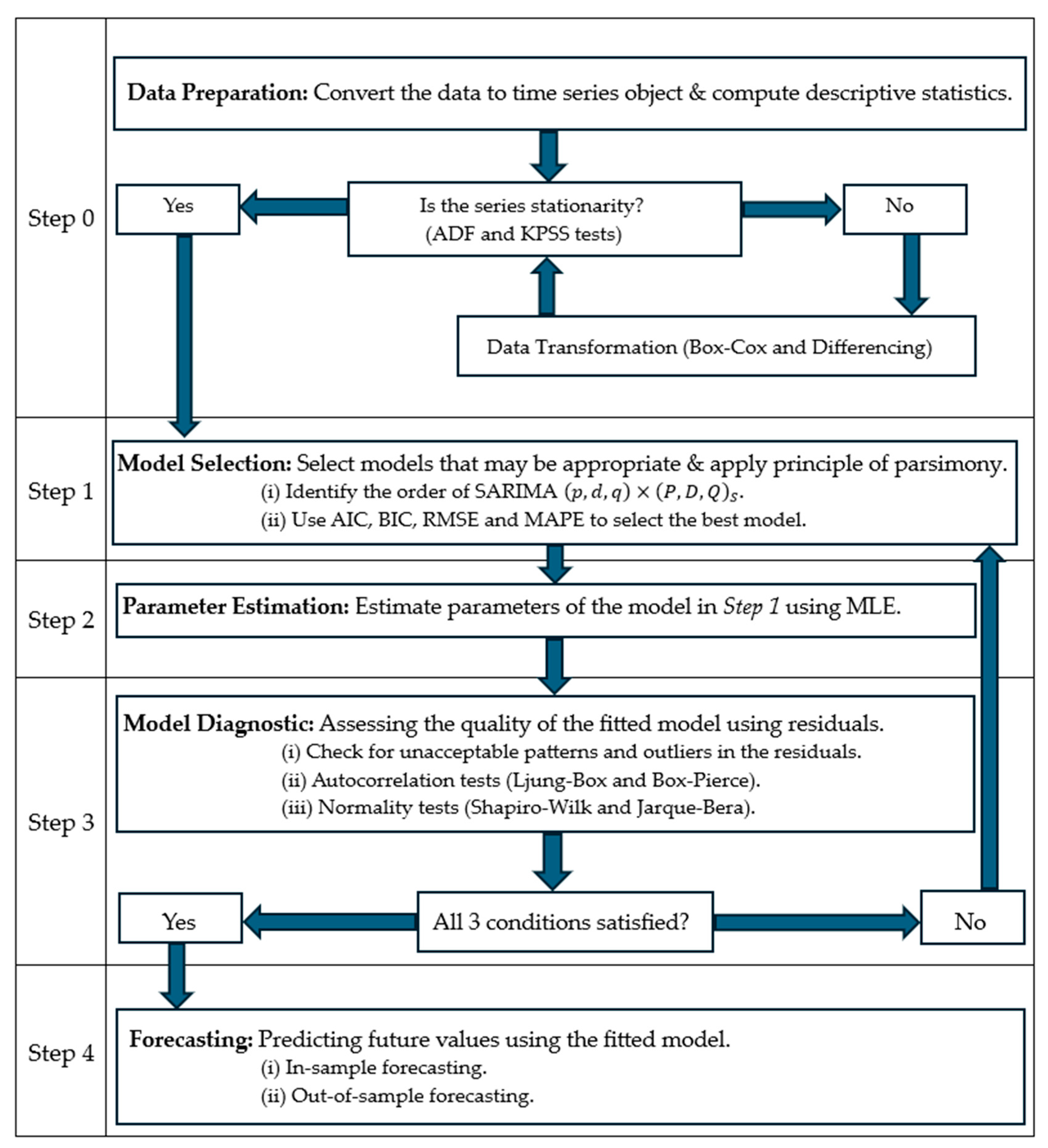
Figure 1. Box–Jenkins methodology outlining data preparation, stationarity, model specification, parameter estimation, and model diagnosis.
Economies 13 00362 g001
Figure 2. Total number of tourist arrivals in South Africa from January 2009 to June 2025, with a reference line in March 2020 denoting the intervention point.
Economies 13 00362 g002
Figure 3. Boxplot of total tourist arrivals in each month during (a) the pre-intervention and (b) intervention periods.
Economies 13 00362 g003
Figure 4. Decomposition plot of A t in the pre-intervention period.
Economies 13 00362 g004
Figure 5. Box–Cox plot of A t in the pre-intervention period.
Economies 13 00362 g005
Figure 6. Plot of 12 A t .
Economies 13 00362 g006
Figure 7. (a) ACF and (b) PACF plots of 12 A t .
Economies 13 00362 g007
Figure 8. (a) Residual plot, (b) ACF, and (c) the histogram of the standardised residuals of SARIMAX 0 , 1 , 1 0 , 1 , 1 12 .
Economies 13 00362 g008
Figure 9. (a) Residual plot, (b) ACF, and (c) the histogram of the standardised residuals of SARIMAX 1 , 1 , 1 0 , 1 , 2 12 .
Economies 13 00362 g009
Figure 10. Actual A t versus fitted A ^ t from the (a) SARIMAX 0 , 1 , 1 0 , 1 , 1 12 and (b) SARIMAX 1 , 1 , 1 0 , 1 , 2 12 models.
Economies 13 00362 g010
Figure 11. Forecasted values of A ^ t from SARIMAX 1 , 1 , 1 0 , 1 , 2 12 .
Economies 13 00362 g011
Figure 12. SARIMAX intervention model augmented with the pulse function covariate vector through trial and error.
Economies 13 00362 g012
Figure 13. Estimated loss in Y t due to the sustained impact of COVID-19.
Economies 13 00362 g013
Figure 14. Forecasted Y ^ t from the SARIMAX intervention model.
Economies 13 00362 g014
Table 1. Model evaluation metrics of fitted SARIMA models before the intervention.
ModelAICBICRMSEMAPE
SARIMA 0 , 1 , 1 0 , 1 , 1 12 2756.592764.9819,319.176.37%
SARIMA 1 , 1 , 2 0 , 1 , 1 12 2758.852772.8319,154.326.41%
SARIMA 2 , 1 , 2 0 , 1 , 1 12 2760.822777.5919,158.696.42%
SARIMA 2 , 1 , 1 2 , 1 , 1 12 2761.692781.2619,188.496.48%
SARIMA 2 , 1 , 2 2 , 1 , 1 12 2763.522785.8919,238.546.30%
SARIMA 0 , 1 , 0 0 , 1 , 1 12 2786.022791.6121,842.576.97%
SARIMA 1 , 1 , 3 0 , 1 , 1 12 2760.832777.6019,157.336.42%
SARIMA 3 , 1 , 1 0 , 1 , 1 12 2760.642777.4219,133.126.42%
SARIMA 4 , 1 , 0 0 , 1 , 1 12 2762.132778.9019,296.846.45%
SARIMA 1 , 1 , 1 0 , 1 , 2 12 2758.802772.7819,163.996.31%
Table 2. Parameter estimates for the SARIMA 0 , 1 , 1 0 , 1 , 1 12 model fitted on A t .
ParametersEstimateStandard Errorz Valuep-Values
θ 1 −0.6186730.079557−7.77657.458 × 10−15
Θ 1 −0.6318000.075798−8.33532.2 × 10−16
Table 3. Parameter estimates of SARIMAX 0 , 1 , 1 0 , 1 , 1 12 .
ParametersEstimateStandard Errorz Valuep-Values
θ 1 −4.0098 × 10−18.2597 × 10−2−4.85461.206 × 10−6
Θ 1 −6.0552 × 10−19.0910 × 10−2−6.66072.726 × 10−11
AO16−3.4850 × 1049.1565 × 103−3.80601.412 × 10−6
AO181.4094 × 1059.4044 × 10314.98642.2 × 10−16
Table 4. Parameter estimates for the SARIMA 1 , 1 , 1 0 , 1 , 2 12 model fitted on A t .
ParametersEstimateStandard Errorz Valuep-Values
ϕ 1 0.1572080.1446421.08690.2771
θ 1 −0.7070520.102821−6.87656.133 × 10−12
Θ 1 −0.6895390.095678−7.20695.725 × 10−13
Θ 2 0.0977810.1285870.76040.4470
Table 5. Parameter estimates of SARIMAX 1 , 1 , 1 0 , 1 , 2 12   .
ParametersEstimateStandard Errorz Valuep-Values
ϕ 1 −8.2420 × 10−11.0910 × 10−1−7.55474.200 × 10−14
θ 1 6.3776 × 10−11.4476 × 10−14.40571.054 × 10−5
Θ 1 −4.4023 × 10−11.1193 × 10−1−3.93318.386 × 10−5
Θ 2 −1.7230 × 10−11.2424 × 10−1−1.38680.1654992
AO16−4.0093 × 1046.2484 × 103−6.41661.394 × 10−10
AO181.3570 × 1056.3495 × 10321.37252.2 × 10−16
AO49−2.7574 × 1046.4845 × 103−4.25222.117 × 10−5
AO76−2.8544 × 1046.2195 × 103−4.58944.445 × 10−6
IO52−1.9628 × 1046.0211 × 103−3.25990.0011146
IO561.4032 × 1046.0853 × 1032.30580.0211197
IO61−2.2002 × 1046.3994 × 103−3.43820.0005857
IO112−2.8725 × 1046.3458 × 103−4.52665.995 × 10−6
Disclaimer/Publisher’s Note: The statements, opinions and data contained in all publications are solely those of the individual author(s) and contributor(s) and not of MDPI and/or the editor(s). MDPI and/or the editor(s) disclaim responsibility for any injury to people or property resulting from any ideas, methods, instructions or products referred to in the content.