The Relationship Between Local Tax Price and Demand of the Public Goods

Abstract

In this study, we use a structural demand framework rather than simple correlations between taxes and expenditure to investigate whether local taxes in Korea function as a price mechanism for local public goods. We construct a panel dataset for 226 basic local governments (cities, counties, and autonomous districts) over the period 2000–2017 and estimate local public expenditure equations separately for each group. To capture both long-run relationships and short-run dynamics while addressing nonstationarity and endogeneity, we combine fully modified ordinary least squares, panel error-correction models, and system generalized method of moments. Across these specifications, local tax burdens—especially when measured as the ratio of per capita local tax to total general expenditure—are generally negatively associated with local expenditure. However, we show that this negative association is distinct from the price elasticity of demand implied by the structural model: the relevant elasticities, derived from the estimated coefficients rather than observed directly, remain positive for cities, counties, and districts. The results indicate that, under Korea’s current intergovernmental fiscal arrangements, local taxes do not operate as a conventional price signal that induces residents to demand less of local public goods when tax price increases. These findings suggest that transfer dependence, limited fiscal autonomy, and rigid expenditure responsibilities weaken the price mechanism of local taxes and have important implications for the design of local tax policy and intergovernmental fiscal equalization.

1. Introduction

Over the past two decades, Korea has experienced a structural shift from high-growth, investment-driven development to a context characterized by slower economic expansion, rapid population aging, and rising demand for welfare and social services. These changes have generated sustained pressure on the finances of both central and local governments, especially basic local governments, which must deliver a broad set of public services with limited independent revenue bases.

In the normative literature on fiscal federalism, local taxes are expected to act as price signals for local public goods. When residents perceive a higher tax price for a given bundle of local services, standard models based on the median voter or the Tiebout sorting model (Tiebout, 1956) predict a reduction in the desired quantity or quality of publicly provided goods. In such a setting, an increase in the local tax price should be associated with a decrease in demand, and the price elasticity of demand for local public goods with respect to the tax price is expected to be negative. As Korea is pursuing decentralization reforms and adjusting its intergovernmental fiscal system, understanding whether local taxes function as price mechanisms has important policy implications. However, the empirical evidence for Korea has been inconsistent.

Some studies report that higher local tax burdens are linked to lower local expenditures, whereas some find weak or statistically insignificant relationships, and others suggest that local taxes do not impose meaningful discipline on spending. A further complication is that earlier research often uses different proxies for “tax price” and typically infers residents’ responsiveness from simple correlations between tax burdens and expenditure levels. This raises two unresolved questions:

First, do local taxes in Korea actually operate as a price mechanism in the sense implied by theory, or do the observed relationships simply reflect the institutional features of the intergovernmental fiscal system, such as strong reliance on grants and equalization transfers? Second, to what extent do previous findings depend on how the tax price is defined and on the choice of econometric method? This study seeks to answer these questions by using two conceptual and methodological approaches.

Conceptually, we carefully distinguish between (i) the association between local tax burdens and local public expenditure and (ii) the price elasticity of demand implied by an estimated demand function for local public goods. Rather than treating any negative coefficient on a tax variable as evidence of a functioning price mechanism, we explicitly derive the elasticity of demand with respect to the tax price and use this elasticity to assess whether local taxes have the expected disciplining role.

Methodologically, we combine three complementary estimation approaches: fully modified ordinary least squares (FMOLS), panel error-correction modeling (ECM), and system generalized method of moments (system GMM). FMOLS is used to identify the long-run equilibrium relationships among expenditure, tax price, income, and other covariates in the presence of possible nonstationarity and cointegration. The ECM captures short-run adjustments toward this long-run equilibrium, whereas the system GMM addresses potential endogeneity and dynamic feedback in a small-T and large-N panel of municipalities. By comparing the behavior of the key coefficients and derived elasticities across these estimators, we can assess whether the main conclusions are robust to alternative specifications and identification strategies.

We analyze an unbalanced panel of 226 basic local governments–cities (si), counties (gun), and autonomous districts (gu)—from 2000 to 2017. This timeframe covers major changes in Korea’s local tax and intergovernmental transfer systems while providing a sufficiently long series to study both long- and short-run dynamics. The study is guided by the following research questions:

• RQ1. When long-run equilibrium and short-run dynamics are considered, how do local tax prices affect local public expenditure in Korean municipalities?
• RQ2. What is the magnitude and sign of the price elasticity of demand for local public goods with respect to local tax prices and does this support the view that local taxes function as an effective price mechanism?
• RQ3. How do these relationships differ across cities, counties, and autonomous districts operating under distinct revenue structures, expenditure responsibilities, and demographic conditions?

By addressing these questions, this study contributes to the Korean literature on fiscal decentralization and the broader debates on local public finance and fiscal federalism. Substantively, it offers a structured reassessment of whether local taxes in Korea transmit meaningful price signals to residents under the current intergovernmental fiscal regime. Methodologically, it illustrates how combining FMOLS, ECM, and system GMM can improve the credibility and interpretability of empirical analyses of local demand for public goods, relative to earlier work that relied on a single estimation technique.

2. Literature Review

Studies on local public finance generally start from the premise that residents choose their preferred level of local public services by weighing the benefits of those services against the tax they must pay to finance them (Bergstrom & Goodman, 1973). In the median voter and Tiebout-style models, each jurisdiction offers a bundle of services and a tax package, and the tax price acts as a signal conveying the marginal cost of local public goods to residents (Oates, 1972).

When this mechanism works as theorized, an increase in the tax price should lead to a reduction in demand for local public goods, and the price elasticity of demand with respect to the tax price is expected to be negative. Translating this theoretical idea into empirical analysis requires a concrete measure of “tax price.” The literature employs a variety of proxies, including local tax revenue per capita, the ratio of local taxes to total revenue, and the ratio of local taxes to total expenditure. Each proxy emphasizes a different aspect of the local fiscal structure and a different channel through which residents may perceive tax burdens, such as the size of the tax base, the degree of tax financing versus transfers, or the share of spending funded by local revenue. In systems with extensive intergovernmental grants, the difference between formal tax instruments and the effective tax price as perceived by residents can be substantial, complicating the interpretation of the estimated coefficients of tax variables.

The Korean literature on local tax prices and local public expenditure is embedded in this broader discussion but also reflects the specific institutional features of Korea’s intergovernmental fiscal system. Earlier Korean studies typically estimated reduced-form demand equations in which local expenditure was regressed on some measure of the local tax burden, income, and demographic controls, often using cross-sectional or static panel data.

Many of these studies adopted per capita local tax revenue or simple tax burden ratios as the main tax price proxy and then interpreted a negative coefficient on this variable as evidence that local taxes perform a price-disciplining function for local public goods. Other studies reported weak, statistically insignificant, or even positive relationships once intergovernmental transfers, fiscal autonomy, and expenditure structure were taken into account, raising doubts about whether local taxes in Korea actually operate as a meaningful price mechanism.

A limitation of much of this research is that it tends to treat any negative correlation between local tax burden and local expenditure as equivalent to a negative price elasticity of demand. In many cases, the estimated coefficient of the tax variable in a reduced-form regression is implicitly interpreted as a measure of price responsiveness, even though the underlying demand function is not explicitly specified and the elasticity is not formally derived. As the reviewer noted, this distinction is crucial: a negative reduced-form coefficient does not necessarily imply negative structural elasticity, especially when the tax variable is embedded in the budget identity. This makes it difficult to distinguish between outcomes driven by genuine demand adjustments and those driven by institutional constraints, grant rules, or other structural features of the fiscal system.

A second limitation pertains to the measurement of tax prices. Korean studies differ in their conceptualization of tax prices in terms of per capita tax, tax-to-revenue ratios, or tax-to-expenditure ratios, and rarely do they systematically compare results across these competing definitions. This heterogeneity is particularly significant in Korea, where intergovernmental transfers, shared taxes, and equalization mechanisms account for a large share of local resources. Depending on which proxy is used, the estimated impact of the tax price may primarily capture changes in local tax bases, in transfer dependence, or in the share of spending financed from own-source revenue, leading to potentially conflicting conclusions about residents’ responsiveness.

A third limitation relates to the econometric approach. Many Korean contributions rely on a single estimation method, most commonly a static fixed effects or random-effects panel model, without fully addressing nonstationarity, cointegration, dynamic adjustment, or endogeneity between tax decisions and expenditure choices. When local governments adjust expenditures gradually over time, and tax and transfer decisions are jointly determined by spending, ignoring dynamics and endogeneity can bias coefficient estimates and obscure the true relationship between tax prices and demand for local public goods.

Recent international research on tax instruments and price responsiveness in other policy areas offers additional insights relevant to the Korean context. Chung and Yoon (2023) investigated tax incentive policies for land use in urban regeneration projects in Korea and showed that local tax incentives can meaningfully alter local socioeconomic conditions, illustrating how local tax design can influence behavioral and spatial outcomes. Liu and Xia (2023) analyze corporate tax rebates and find that tax refunds can improve firms’ total factor energy productivity, suggesting that carefully designed tax instruments can induce efficiency-enhancing responses. Kusumastuti (2022) evaluated sales tax incentives on luxury goods in Indonesia during the COVID-19 pandemic and reported that the effectiveness of such measures depended strongly on macroeconomic conditions and implementation details.

In commodity and resource markets, Pratama et al. (2024) studied price competition and shifting demand between palm and coconut oil exports, while Vidal-Lamolla et al. (2024) used social simulations to estimate how residential water demand responds to price changes. Taken together, the findings of these studies confirm that tax and price instruments can shape demand and behavior but also show that the magnitude and sign of responses are highly context-dependent and mediated by institutional and market structures (Chung & Yoon, 2023; Liu & Xia, 2023; Kusumastuti, 2022; Pratama et al., 2024; Vidal-Lamolla et al., 2024).

This broader evidence underscores the fact that the relationship between tax prices and the demand for publicly provided goods cannot be assumed to follow a universal pattern; it must be examined empirically within each country’s fiscal architecture.

In Korea, where local governments combine formal tax authorities with a substantial reliance on central transfers and equalization, it is an open question whether residents perceive local taxes as a clear price signal for the services they receive.

Against this backdrop, this study contributes to the literature in three ways. First, at the conceptual level, we move beyond simple correlations between the tax burden and expenditure by explicitly specifying a demand function for local public goods and deriving the price elasticity of demand with respect to the local tax price from the estimated coefficients. This allows us to distinguish between cases where local tax variables are negatively correlated with expenditure and cases in which residents exhibit genuine price-responsive demand behavior, consistent with the theoretical notion of a functioning price mechanism.

Second, at the methodological level, we address the limitations of single-method analyses by combining fully modified ordinary least squares (FMOLS), panel ECM, and system generalized method of moments (system GMM). FMOLS is used to identify long-run equilibrium relationships among expenditure, tax price, income, and other determinants in the presence of possible nonstationarity and cointegration. The ECM captures short-run adjustments of the long-run equilibrium, including the speed at which local expenditures respond to deviations from that equilibrium. System GMM addresses potential endogeneity and dynamic feedback by using lagged levels and differences in explanatory variables as instruments in a small-T, large-N municipal panel. By comparing the behavior of key coefficients and derived elasticities across these estimators, we can assess whether the core findings are robust to alternative identification strategies and dynamic specifications.

Third, at the substantive level, we place Korea within the broader debate on fiscal decentralization and intergovernmental finance. Korea’s combination of local tax autonomy, strong grant systems, and pronounced differences among cities, counties, and districts creates a setting in which the price role of local taxes is theoretically plausible, but empirically uncertain. By examining how tax prices, local expenditures, and the derived price elasticity of demand vary across these types of basic local governments, this study provides evidence of whether and under what conditions local taxes in Korea function as a price mechanism for local public goods.

3. Stylized Facts About Revenue of Local Governments

Local autonomy was restored to Korea in the early 1990s and began to operate in earnest with the introduction of direct elections for local government heads in 1995 (Ministry of the Interior and Safety, various years). The current local government system is organized into two tiers: upper-level metropolitan governments and lower-level basic local governments. Metropolitan governments consist of eight metropolitan cities (including the special metropolitan city) and nine provinces, while basic local governments comprise cities (si), counties (gun), and autonomous districts (gu) established under these upper-level jurisdictions.

During the study period, there were 226 basic local governments, including 75 cities, 69 districts, and 82 counties. From a fiscal perspective, the revenues of Korean local governments can be broadly divided into own-source and intergovernmental revenues (Ministry of the Interior and Safety, various years). Intergovernmental revenues are resources for which local governments do not hold direct taxation or collection authority. Instead, they are provided by the central government or higher-level local governments. These include local allocation taxes (ordinary and special grants), shared taxes, specific-purpose subsidies from the central government, adjustment grants, and municipal subsidies from metropolitan and provincial governments.

Own-source revenue consists of local and non-tax revenues. Non-tax revenues encompass all revenues other than local taxes, such as user charges and fees, property rental income, fines, and miscellaneous receipts. These are often classified as ordinary non-tax revenues, which accrue regularly and are relatively predictable for each fiscal year, and one-off non-tax revenues, which arise irregularly from asset sales or other exceptional transactions. Within this category, ordinary non-tax revenues such as usage fees, commissions, and rental income play a significant role in supplementing local fiscal resources, although their overall magnitude is generally smaller than that of local taxes.

Local taxes are defined and regulated by the Local Tax Act, which specifies the taxable items, tax bases, and statutory rates. During the period analyzed in this study, the local tax system comprised eleven major tax items, which can be grouped by the level of government into provincial taxes and city/county/district taxes.

Provincial taxes imposed and collected by metropolitan governments include acquisition, registration and licensing, leisure, local consumption, regional resources and facilities, and local education taxes. City and county taxes levied and collected by basic local governments include tobacco consumption, resident, local income, property, and automobile taxes, whereas autonomous districts are responsible for imposing and collecting property, registration, and license taxes.

From an economic perspective, these tax items can also be classified into property, income, consumption, and other taxes. Property-related taxes include acquisition tax, property tax, automobile tax on ownership, and the portion of regional resources and facilities tax that applies to specific real-estate holdings. The local income tax represents the income tax component, whereas local consumption, tobacco consumption, and leisure taxes, and the automobile tax on use (driving) are categorized as consumption taxes. Other taxes include local education tax, registration and license tax, resident tax, and the portion of the regional resources and facilities tax that applies to specific resource use.

Descriptive statistics for 2000–2017 reveal substantial variations in financial independence across different types of local governments. Financial independence is typically measured as the ratio of own-source revenue to total general account revenue. Over the study period, the average financial independence rate for all local governments was approximately 54%, with metropolitan cities (including the special metropolitan city) recording around 73%, and provincial governments approximately 36%. Among basic local governments, the average financial independence rate was approximately 40% for cities, 17% for counties, and 38% for districts, indicating that basic local governments, particularly counties, rely much more heavily on transfers than metropolitan governments. These patterns highlight the relatively limited dependence on own-source revenue among many basic local governments (see Figure 1).

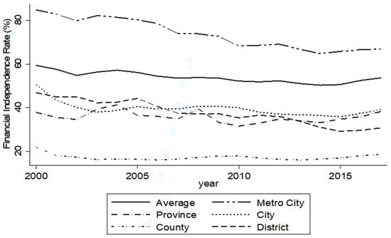
Figure 1. Financial Independence rate of Korea Local Government (2000–2017).

The evolution of local tax revenue over time shows marked expansion. All figures reported in this section reflect nominal values, unless otherwise stated. Between 2000 and 2017, the total local tax revenue increased by approximately 290%, reaching approximately 79.8 trillion KRW 2017. Growth rates differed across government types; provincial taxes increased by approximately 414% during this period, city taxes increased by approximately 326%, and metropolitan taxes increased by approximately 251%. In 2017, metropolitan taxes accounted for around 42% of total local tax revenue (33.1 trillion KRW), followed by provincial taxes at 28% (22.5 trillion KRW), city taxes at 22% (17.8 trillion KRW), district taxes at 5% (4.2 trillion KRW), and county taxes at 3% (2.2 trillion KRW). These figures indicate that while local tax revenues have grown substantially, the tax base of basic local governments—cities, districts, and counties—remains relatively modest compared to that of metropolitan governments (see Figure 2).

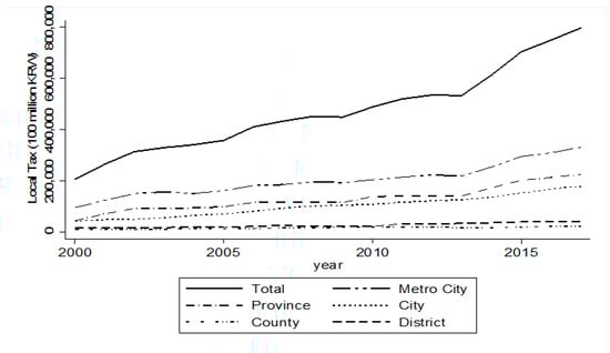
Figure 2. Growth of Local Tax revenues (2000–2017).

The 2011 local tax system reform was an important institutional development during the study period. As part of this reform, local consumption tax and local income tax were introduced or restructured, with the aim of reducing the previous concentration of local taxation on property and moving toward a more balanced mix of property, consumption, and income taxes (Ministry of Economy and Finance, various years). The reform was intended to strengthen local tax bases, improve fairness, and better align local revenue structures with patterns of economic activity.

Local tax revenues also increased relative to the size of the national economy. The ratio of total local taxes to gross domestic product (GDP) increased from approximately 3.1% in 2000 to 4.3% in 2017, indicating a gradual upward trend in the local tax share of GDP over the period. During these years, the contribution of metropolitan, provincial, city, county, and district taxes to the total local tax/GDP ratio have differed, with metropolitan and provincial taxes accounting for the largest proportion (see Figure 3).

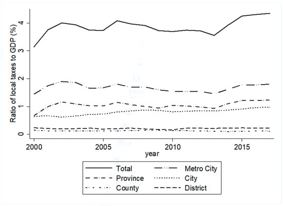
Figure 3. Ratio of Local Taxes to GDP (2000–2017).

These stylized facts are directly relevant for the empirical analysis that follows. The relatively low financial independence of many basic local governments and their heavy reliance on intergovernmental transfers suggest that residents may not perceive changes in local taxes as fully proportional to changes in the “price” of local public services. Furthermore, substantial cross-sectional differences in revenue structures across cities, counties, and districts imply that the impact of local tax prices on expenditure and the resulting price elasticity of demand for local public goods may vary systematically according to the type of local government. Against this background, the next section develops an econometric model in which tax price is defined as the share of expenditure financed by local taxes and estimates how this tax price is related to the demand for local public goods in different categories of basic local governments.

4. Econometric Model

The empirical specification in this study is based on the standard model of local public good demand developed by Bergstrom and Goodman (1973), in which a representative or median voter chooses the level of a congestible local public good. When congestion is present, the quantity of the public good effectively available to each individual $Z^{*}$, is defined as

$$Z^{*}={\displaystyle \frac{Z}{N^r}}$$

(1)

Here, $Z$ denotes the total quantity of the local public good supplied, $N$ is the number of residents consuming the public good, and $r\in \left[\mathrm{0,1}\right]$ is a congestion parameter.

If $r=0$, the good behaves as a pure-public good, whereas $r=1$ corresponds to a purely private good; intermediate values reflect varying degrees of crowding.

The median voter derives utility from a private composite good $X_i$ and the effective quantity of the local public good $Z^{*}$, and faces the following budget constraint under the simplifying assumption that the price of the private good is normalized to one:

$$\begin{gathered} \hspace{1em}\hspace{1em}Max U_i\left(X_i,Z^{*}\right) \\ s.t.X_i+{\tau }_{i}qZ\le Y_i \end{gathered}$$

(2)

In (2), $q$ is the unit cost of providing the public good, ${\tau }_i$ is the share of the total tax burden borne by individual $i$, and $Y_i$ denotes the income of the median voter. The term ${\tau }_{i}qZ$ represents the tax payment required from the median voter to finance the chosen level of the public good.

Bergstrom and Goodman (1973) show that, under the assumption of constant income and price elasticities of demand, $\delta$ and $e$ respectively, the individual demand for the local public good can be written as:

$$Z^{*}={c\left\{{\tau }_{i}q{N}^r\right\}}^{\delta }{Y}_i^e$$

(3)

where $c$ is a positive constant.

Aggregating across residents yields the total demand for the local public good:

$$Z^{*}=c{{\tau }_i}^{\delta }{q}^{\delta }{N}^{r(1+\delta )}{Y}_i^e$$

(4)

Taking logarithms of both sides leads to the following log-linear demand equation:

$${lnZ}^{*}=\mathrm{l}\mathrm{n}\mathrm{c}+\mathsf{\delta }\mathrm{l}\mathrm{n}{\tau }_{i}q+r\left(1+\delta \right)lnN+eln{Y}_i$$

(5)

On this basis, the demand function to be estimated for local government $j$ of type $k$ can be written as:

$${lnZ}_j^k={\mathsf{\beta }}_{k0}+{\mathsf{\alpha }}_{k1}{\mathrm{l}\mathrm{n}\mathrm{T}}_j^k+{\mathsf{\beta }}_{k2}{\mathrm{l}\mathrm{n}\mathrm{N}}_j^k+{\mathsf{\beta }}_{k3}{\mathrm{l}\mathrm{n}\mathrm{Y}}_j^k+{ϵ}_k$$

(6)

However, in reality, there are no data indicating demand for public good as a dependent variable in (6); thus, expenditure data on public good are used to replace demand for public good. According to Bergstrom and Goodman (1973), the unit cost of local public good is constant. However, in reality, there are no data indicating demand for public goods as a dependent variable, so expenditure data on public goods are used to replace demand for public goods.

$$\begin{gathered} ln{E}_j={ln{T}_{j}Z}_j^k=ln{T}_j+{lnZ}_j^k \\ ={ln{T}_j+\mathsf{\beta }}_{k0}+{\mathsf{\beta }}_{k1}{\mathrm{l}\mathrm{n}\mathrm{T}}_j^k+{\mathsf{\beta }}_{k2}{\mathrm{l}\mathrm{n}\mathrm{N}}_j^k+{\mathsf{\beta }}_{k3}{\mathrm{l}\mathrm{n}\mathrm{Y}}_j^k+{ϵ}_k \\ {=\mathsf{\beta }}_{k0}+({\mathsf{\beta }}_{k1}+1){\mathrm{l}\mathrm{n}\mathrm{T}}_j^k+{\mathsf{\beta }}_{k2}{\mathrm{l}\mathrm{n}\mathrm{N}}_j^k+{\mathsf{\beta }}_{k3}{\mathrm{l}\mathrm{n}\mathrm{Y}}_j^k+{ϵ}_k \\ \because \mathrm{l}\mathrm{n}\mathrm{E}=\mathrm{l}\mathrm{n}\mathrm{q}+\mathrm{l}\mathrm{n}\mathrm{Z},\mathrm{E}=\mathrm{q}\mathrm{Z} \end{gathered}$$

(7)

In Equation (7), the coefficient $\left({\beta }_{k1}+1\right)$ on $\ln T_j^k$ can be interpreted as the elasticity of local public expenditure with respect to the tax-price variable, under the maintained assumption of constant unit cost. This provides a basis for deriving the implied price elasticity of demand for local public goods from the estimated expenditure equation.

To link the theoretical tax share ${\tau }_i$ to observable fiscal variables, we follow Joo (2010), who critically reviewed the original Bergstrom–Goodman formulation and proposed measuring the tax price as the ratio of per capita local tax revenue to total general expenditure. The underlying assumption is that the median voter bears the average local tax burden, so that ${\tau }_i$ can be approximated by the per capita local tax divided by total expenditure.

Formally, the tax price can be written as:

$${\tau }_i={\displaystyle \frac{T_i}{qZ}}={\displaystyle \frac{T_i}{E}}\approx {\displaystyle \frac{\raisebox{1ex}{$\sum _{i=1}^n{T}_i$}\!\left/ \!\raisebox{-1ex}{$n$}\right.}{E}}$$

(8)

where $T_i$ denotes per capita local tax revenue, and $E$ is total general expenditure.

We adopt this ratio as a proxy for the tax price faced by residents and compare it with alternative specifications based on the per capita local tax. All expenditure, tax, and income variables in the empirical model are expressed in real terms (2015 constant KRW).

For the income variable, we follow Won (2008), who argues that wages in mining and manufacturing provide a more appropriate proxy for residents’ income than gross regional domestic product (GRDP) because GRDP refers to the total value added produced in the region rather than the income accrued to local residents. In addition to tax price and income, the model includes demographic controls, such as the elderly population ratio and population (and, where relevant, population growth), as commonly suggested in the literature on local public goods demand and social service needs.

As noted earlier, local governments in Korea are divided into three groups: cities, counties, and autonomous districts, and demand equations are estimated separately for each group. This reflects the substantial differences in revenue structures and expenditure responsibilities across basic local governments. For example, cities obtain a sizable portion of their revenue from equalization transfers, whereas districts do not receive ordinary allocation tax directly. However, the local tax items assigned to each type of government differ, which may lead to heterogeneous responses to changes in local tax burdens and tax price. To capture these features explicitly, we specify the following log-linear expenditure equations for local government $j$ of type $k$ in year $t$.

The first specification uses per capita local tax as the key fiscal variable:

$${lnE}_{j,t}^k={\mathsf{\alpha }}_{k0}+{\mathsf{\alpha }}_{k1}{\mathrm{l}\mathrm{n}\mathrm{T}}_{j,t}^k+{\mathsf{\alpha }}_{k2}{\mathrm{l}\mathrm{n}\mathrm{Y}}_{j,t}^k+{\mathsf{\alpha }}_{k3}{\mathrm{l}\mathrm{n}\mathrm{N}}_{j,t}^k+{\mathsf{\alpha }}_{k4}{\mathrm{l}\mathrm{n}\mathrm{O}}_{j,t}^k+{\mathsf{\alpha }}_{k5}D+{ϵ}_{k,t}$$

(7a)

The second specification uses the tax-price ratio $P_{j,t}^k$, defined as per capita local tax divided by total general expenditure, as the main explanatory variable.

$${lnE}_{j,t}^k={\mathsf{\beta }}_{k0}+{\mathsf{\beta }}_{k1}{\mathrm{l}\mathrm{n}\mathrm{P}}_{j,t}^k+{\mathsf{\beta }}_{k2}{\mathrm{l}\mathrm{n}\mathrm{Y}}_{j,t}^k+{\mathsf{\beta }}_{k3}{\mathrm{l}\mathrm{n}\mathrm{N}}_{j,t}^k+{\mathsf{\beta }}_{k4}{\mathrm{l}\mathrm{n}\mathrm{O}}_{j,t}^k+{\mathsf{\beta }}_{k5}D+{\mu }_{k,t}$$

(7b)

In (7a) and (7b), $E_{j,t}^k$ denotes per capita general account expenditure of local government $j$ of type $k$ in year $t$; $T_{j,t}^k$ is per capita local tax revenue; $P_{j,t}^k$ is the tax price, measured as the ratio of per capita local tax to total general expenditure; $Y_{j,t}^k$ is the income proxy; $N_{j,t}^k$ is population; $O_{j,t}^k$ is the share of elderly residents; and $D_t$ is is a dummy variable capturing the structural reform of the local tax system, taking the value 0 before 2011 and 1 from 2011 onwards. The error terms ${\epsilon }_{j,t}^k$ and ${\mu }_{j,t}^k$ capture unobserved factors affecting expenditure.

The panel used in the empirical analysis covers 2000–2017 and includes 67 cities, 79 counties, and 69 districts, yielding a small-T and large-N panel. This structure, combined with potential nonstationarity, long-run relationships, and endogeneity between tax variables and expenditure, motivates the use of multiple complementary estimators in the subsequent analysis, namely, fully modified OLS (FMOLS), panel ECM, and system GMM, to obtain robust estimates of the effects of tax price and to derive the implied price elasticities of demand.

5. Estimation Result

5.1. Data

The empirical analysis was designed to test whether local tax price operates as a genuine price signal for local public good in Korea. To capture potential heterogeneity in fiscal structure and expenditure responsibilities, the sample is divided into three groups of basic local governments—cities (si), counties (gun), and autonomous districts (gu)—and the demand equations are estimated separately for each group, as specified in Equation (7a,b).

The dataset is an unbalanced panel covering 2000–2017 for all basic local governments subject to data availability. During this period, there were 226 basic local governments (75 cities, 82 counties, and 69 districts), although the number of observations by year and jurisdiction may have varied slightly because of missing values.

The starting year was determined by the availability of consistent local finance statistics at the municipal level, and the end year was chosen to ensure data completeness prior to more recent institutional changes while still covering the 2011 reform of the local tax system discussed above (Ministry of the Interior and Safety, various years; Ministry of Economy and Finance, various years). All fiscal and demographic variables are constructed using official statistics published by the Ministry of Interior and Safety and related central government agencies. All the fiscal variables used in the empirical analysis were converted into real terms using 2015 as the base year.

The key dependent variable is the per capita general account expenditure of each local government, which is used as a proxy for demand for local public goods under the assumption of a constant unit cost of provision. The main fiscal explanatory variables are per capita local tax revenue and tax price, defined as the ratio of per capita local tax revenue to the total general account expenditure of each local government. The latter follows the interpretation of tax price as the share of expenditure financed by local taxes (Bergstrom & Goodman, 1973; Joo, 2010).

The income variable was measured as the per capita wage in the mining and manufacturing sectors, which has been suggested as a more appropriate proxy for residents’ income than gross regional domestic product (GRDP), since GRDP refers to total production in the region rather than the income accrued to residents (Won, 2008). Demographic controls included the population size of each jurisdiction and the ratio of older adults to population, which captures differences in age structure and associated expenditure needs, particularly for welfare and social services.

For the estimation, all continuous variables were transformed into natural logarithms: log expenditure, log of local tax per capita, log tax price, log income, log population, and (where appropriate) log older adult population ratio. This transformation facilitated the interpretation of the estimated coefficients as elasticities and mitigated the influence of outliers. In addition, a dummy variable for the 2011 local tax reform was included to capture the structural changes in the local tax system during the sample period.

Table 1 reports descriptive statistics for all variables used in the empirical analysis, by pooling observations across cities, counties, and districts. The table summarizes the mean, standard deviation, minimum, and maximum values, and thereby provides an overview of the substantial cross-sectional and temporal variation that underlies the subsequent estimation.

Table 1. Basic Statistics of variables.

	Cities (k = 1)
	${\mathit{E}}_{\mathit{k},\mathit{t}}$ (Billion KRW)	${\mathit{T}}_{\mathit{k},\mathit{t}}$ (Thousand KRW)	${\mathit{P}}_{\mathit{k},\mathit{t}}$	${\mathit{Y}}_{\mathit{k},\mathit{t}}$ (Million KRW)	${\mathit{N}}_{\mathit{k},\mathit{t}}$ (Billion KRW)	${\mathit{O}}_{\mathit{k},\mathit{t}}$
Mean	483.6	785.5	0.02	28.6	293,270.8	0.12
Median	417.9	690.2	0.01	26.6	210,391.5	0.11
Maximum	1988.3	9270.6	0.51	84.3	1,202,628.0	0.36
Minimum	65.6	127.6	0.00	9.4	45,888.0	0.04
Std. Dev.	302.3	847.0	0.04	10.9	240,770.9	0.05
Skewness	1.7	6.5	9.48	1.3	1.6	0.97
Kurtosis	6.8	57.0	99.13	5.9	5.0	3.61
	Counties (k = 2)
Mean	241.4	595.7	0.02	24.5	3380.2	0.22
Median	231.1	529.6	0.02	21.0	1177.0	0.22
Maximum	859.4	2217.5	0.08	1420.0	41,286.0	0.38
Minimum	38.1	82.9	0.00	4.8	38.0	0.07
Std. Dev.	101.9	395.1	0.01	51.8	6238.9	0.06
Skewness	0.1	9.9	0.90	0.0	3.2	−0.02
Kurtosis	0.4	37.6	3.99	0.0	13.5	2.33
	Districts (k = 3)
Mean	230.3	759.4	0.03	24.6	3380.2	0.22
Median	201.4	517.1	0.02	22.2	4231.0	0.09
Maximum	759.5	10,056.0	0.38	88.5	67,051.0	0.24
Minimum	33.8	6.9	0.00	7.8	67.0	0.03
Std. Dev.	129.7	1091.3	0.05	11.2	13,972.1	0.04
Skewness	0.1	44.7	3.99	0.0	1.9	0.77
Kurtosis	0.3	296.3	22.60	0.0	6.0	3.33

5.2. Panel Unit Root and Panel Cointegration

Because the empirical analysis was based on panel data combining time and cross-sectional dimensions, it was essential to examine the time-series properties of the variables before estimating the demand equations. In particular, the presence of unit roots and the possibility of cointegration had important implications for the validity of standard regression results and for the choice of estimators such as FMOLS and error-correction models.

First, we conducted panel unit root tests for all the variables. In the panel data literature, unit root tests are typically classified into those that assume a common unit root process across cross-sectional units, and those that allow for individual-specific unit root processes. As a representative common-process test, we employed the Levin–Lin–Chu (LLC) test (Levin et al., 2002), while for heterogeneous processes we used the Im–Pesaran–Shin (IPS) test (Im et al., 2003) and the Fisher-type tests based on augmented Dickey–Fuller (ADF) and Phillips–Perron (PP) statistics proposed by Maddala and Wu (1999).

As noted by Baltagi (2008), the LLC and IPS tests are more reliable when the time dimension $T$ is relatively large compared with the cross-sectional dimension $N$.

Given the structure of our dataset, we placed particular emphasis on the Fisher-type ADF and PP statistics, which are well suited for panels with moderate $T$ and a larger number of cross-sectional units. The detailed results of the panel unit root tests are presented in Table 2.

Table 2. Results of the Panel Unit Root Test.

		Cities (k = 1)		Counties (k = 2)		Districts (k = 3)
Common Unit Root		Level	Difference	Level	Difference	Level	Difference
	$\ln E_{k,t}$	−10.37 ***	−25.93 ***	−13.78 ***	−31.30 ***	−4.82 ***	−32.15 ***
	$\ln T_{k,t}$	−9.34 ***	−23.30 ***	−11.59 ***	−26.12 ***	6.74	−28.13 ***
	$\ln P_{k,t}$	−9.94 ***	−26.44 ***	−14.59 ***	−31.91 ***	−7.43 ***	−27.05 ***
	$ln{Y}_{k,t}$	−2.93 ***	−20.96 ***	−5.14 ***	−26.67 ***	−7.66 ***	−24.39 ***
	$ln{N}_{k,t}$	−12.86 ***	−11.15 ***	−28.41 ***	−10.41 ***	−5.96 ***	−14.57 ***
	$\ln O_{k,t}$	−16.49 ***	−8.21 ***	−37.99 ***	−7.06 ***	−7.59 ***	−10.98 ***
Individual Unit Root		Level	Difference	Level	Difference	Level	Difference
IPS	$\ln E_{k,t}$	−1.18	−181.14 ***	−6.17 ***	−22.31 ***	5.68	−21.98 ***
	$\ln T_{k,t}$	0.98	−15.98 ***	−0.65	−18.23 ***	10.67	−17.14 ***
	$\ln P_{k,t}$	−6.81 ***	−20.01 ***	−11.13 ***	−24.92 ***	−2.04 **	−16.62 ***
	$ln{Y}_{k,t}$	4.10	−16.01 ***	2.66	−20.74 ***	−3.36 ***	−18.32 ***
	$ln{N}_{k,t}$	−4.55 ***	−7.49 ***	−15.24 ***	−7.68 ***	−1.05	−10.40 ***
	$\ln O_{k,t}$	−6.38 ***	−5.47 ***	−22.11 ***	−2.62 ***	3.56	−6.88 ***
ADF	$\ln E_{k,t}$	117.69	500.2 ***	185.15 **	696.60 ***	50.88	654.69 ***
	$\ln T_{k,t}$	84.61	444.36 ***	156.08	585.81 ***	70.37	510.06 ***
	$\ln P_{k,t}$	245.90 ***	551.72 ***	394.64 ***	771.88 ***	160.28 *	505.54 ***
	$ln{Y}_{k,t}$	83.00	449.17 ***	135.22	652.91 ***	222.25 ***	555.39 ***
	$ln{N}_{k,t}$	229.78 ***	251.44 ***	500.78 ***	336.02 ***	179.19 **	339.89 ***
	$\ln O_{k,t}$	248.66 ***	207.49 ***	681.34 ***	206.84 ***	97.54	249.63 ***
PP	$\ln E_{k,t}$	226.02 ***	643.75 ***	309.89 ***	1054.13 ***	61.79	869.92 ***
	$\ln T_{k,t}$	142.05 *	475.75 ***	192.07	690.86 ***	69.63	563.24 ***
	$\ln P_{k,t}$	250.82 ***	829.42 ***	501.27 ***	1115.72 ***	160.63 *	581.41 ***
	$ln{Y}_{k,t}$	107.21	571.86 ***	203.71	822.44 ***	230.43 ***	720.86 ***
	$ln{N}_{k,t}$	254.94 ***	285.17 ***	623.86 ***	379.34 ***	184.87 ***	396.26 ***
	$\ln O_{k,t}$	375.61 ***	176.88 ***	1039.41 ***	217.53 ***	184.09 ***	235.66 ***

Notes: ***, **, and * reject the hypotheses at the 1%, 5%, and 10% significance levels, respectively.

The unit root tests indicate that the main variables cannot always be treated as stationary in levels, whereas their first differences generally reject the null hypothesis of a unit root at conventional significance levels. In other words, the key variables behaved as integrated of order one, $I\left(1\right)$, processes. This pattern is consistent with the use of cointegration techniques and motivates the subsequent residual-based cointegration analysis.

Because the reliability of the LLC and related tests depended on the assumption of cross-sectional independence, we also examined whether there was significant cross-sectional dependence among the local governments in our panel. For this purpose, we applied several widely used test statistics: the Breusch–Pagan LM test (Breusch & Pagan, 1980), the scaled LM and CD tests proposed by Pesaran (2004), and the bias-corrected scaled LM statistic developed by Baltagi et al. (2012). The results summarized in Table 3, do not indicate strong cross-sectional dependence for the variables considered, suggesting that the assumption of weak cross-sectional correlation is reasonable in this setting.

Table 3. Results of Cross-Sectional Dependence Test.

		Cities (k = 1)	Counties (k = 2)	Districts (k = 3)
Breusch–Pagan LM
	$\ln E_{k,t}$	35,188.2 ***	45,964.2 ***	40,537.7 ***
	$\ln T_{k,t}$	36,239.9 ***	49,920.1 ***	39,001.5 ***
	$\ln P_{k,t}$	21,162.5 ***	30,738.0 ***	35,691.5 ***
	$ln{Y}_{k,t}$	33,901.8 ***	37,600.8 ***	31,787.0 ***
	$ln{N}_{k,t}$	16,505.0 ***	17,885.1 ***	18,750.7 ***
	$\ln O_{k,t}$	38,162.9 ***	53,369.2 ***	40,655.8 ***
Scaled LM
	$\ln E_{k,t}$	495.9 ***	546.3 ***	557.6 ***
	$\ln T_{k,t}$	511.7 ***	596.7 ***	535.1 ***
	$\ln P_{k,t}$	285.0 ***	352.3 ***	486.8 ***
	$ln{Y}_{k,t}$	476.6 ***	439.8 ***	429.8 ***
	$ln{N}_{k,t}$	215.0 ***	188.6 ***	239.5 ***
	$\ln O_{k,t}$	540.6 ***	640.6 ***	559.3 ***
Bias-corrected scaled LM
	$\ln E_{k,t}$	493.9 ***	544.0 ***	555.5 ***
	$\ln T_{k,t}$	509.8 ***	594.4 ***	533.1 ***
	$\ln P_{k,t}$	283.0 ***	350.0 ***	484.8 ***
	$ln{Y}_{k,t}$	474.6 ***	437.4 ***	427.8 ***
	$ln{N}_{k,t}$	213.0 ***	186.3 ***	237.5 ***
	$\ln O_{k,t}$	538.7 ***	638.3 ***	557.3 ***
Pesaran CD
	$\ln E_{k,t}$	187.0 ***	212.5 ***	201.3 ***
	$\ln T_{k,t}$	190.2 ***	223.1 ***	197.2 ***
	$\ln P_{k,t}$	140.3 ***	170.6 ***	188.4 ***
	$ln{Y}_{k,t}$	182.7 ***	187.3 ***	176.3 ***
	$ln{N}_{k,t}$	57.7 ***	44.2 ***	48.5 ***
	$\ln O_{k,t}$	195.2 ***	230.9 ***	199.9 ***

Note: The null hypothesis is that the residuals across cross-entities are not correlated. ***, **, and * denote significance at the 1%, 5%, and 10% levels respectively.

Using nonstationary variables in levels without cointegration may lead to spurious regression results. To assess whether a stable long-run relationship exists among the variables in the expenditure equations, we conduct panel residual cointegration tests. Specifically, we employ the tests proposed by Pedroni (1999, 2000), which allow for considerable heterogeneity across cross-sectional units, and the test developed by Kao (1999), who uses a homogeneous panel framework.

The Pedroni statistics provide mixed evidence, with some statistics rejecting the null hypothesis of no cointegration and others not rejecting it at conventional levels (see Table 4).

Table 4. Results of residual cointegration test proposed by Pedroni (1999, 2000).

	Cities (k = 1)		Counties (k = 2)		Districts (k = 3)
Within-Dimension	7a	7b	7a	7b	7a	7b
Panel v-Statistic	−1.53	−1.09	2.33 ***	0.28	−2.06	−1.63
Panel rho-Statistic	1.80	2.72	−0.34	1.17	3.65	3.24
Panel pp-Statistic	−11.26 ***	−8.56 ***	−11.92 ***	−6.80 ***	−7.62 ***	−7.02 ***
Panel ADF-Statistic	−11.88 ***	−9.50 ***	−13.14 ***	−7.70 ***	−10.86 ***	−8.99 ***
Between-Dimension	7a	7b	7a	7b	7a	7b
Group rho-Statistic	5.07	5.54	2.87	3.85	7.46	7.23
Group pp-Statistic	−19.20 ***	−16.40 ***	−15.44 ***	−9.21 ***	−13.05 ***	−13.73 ***
Group ADF-Statistic	−15.42 ***	−14.24 ***	−15.41 ***	−9.83 ***	−13.90 ***	−12.68 ***

Note: The null hypothesis is that the variables are not cointegrated. ***, **, and * denote significance at the 1%, 5%, and 10% levels respectively.

By contrast, the Kao test clearly rejects the null of no cointegration, indicating the presence of a cointegrating relationship among expenditure, tax price (or tax level), income, population, and the other controls (see Table 5). Taken together, these results support the view that the main variables are cointegrated, which justifies the use of FMOLS to estimate long-run coefficients and the specification of ECM to capture short-run adjustment dynamics in the subsequent empirical analysis.

Table 5. Results of the residual cointegration test.

	Cities (k = 1)		Counties (k = 2)		Districts (k = 3)
	7a	7b	7a	7b	7a	7b
Group ADF-Statistic	−8.73 ***	−11.67 ***	−15.88 ***	−10.13 ***	−7.65 ***	−6.75 ***

Note: The null hypothesis is that the variables are not cointegrated. ***, **, and * denote significance at the 1%, 5%, and 10% levels.

5.3. Empirical Results

This section presents the empirical results obtained from the three-step estimation strategy outlined above: (i) long-run estimation using FMOLS under the assumption of cointegration, (ii) short-run estimation using panel ECM, and (iii) dynamic estimation using system GMM to address potential endogeneity in a small-$T$, large-$N$ setting.

5.3.1. Long-Run Fully Modified Ordinary Least Squares Estimates

Given the evidence of cointegration among the main variables, we first estimated the long-run expenditure equations using FMOLS as proposed by Pedroni (2000).

Specifically, Equation (7a,b) were estimated in their long-run forms as follows:

$${lnE}_{j,t}^k={\mathsf{\alpha }}_{k0}+{\mathsf{\alpha }}_{k1}{\mathrm{l}\mathrm{n}\mathrm{T}}_{j,t}^k+{\mathsf{\alpha }}_{k2}{\mathrm{l}\mathrm{n}\mathrm{Y}}_{j,t}^k+{\mathsf{\alpha }}_{k3}{\mathrm{l}\mathrm{n}\mathrm{N}}_{j,t}^k+{\mathsf{\alpha }}_{k4}{\mathrm{l}\mathrm{n}\mathrm{O}}_{j,t}^k+{ϵ}_{k,t}$$

(8a)

$${lnE}_{j,t}^k={\mathsf{\beta }}_{k0}+{\mathsf{\beta }}_{k1}{\mathrm{l}\mathrm{n}\mathrm{P}}_{j,t}^k+{\mathsf{\beta }}_{k2}{\mathrm{l}\mathrm{n}\mathrm{Y}}_{j,t}^k+{\mathsf{\beta }}_{k3}{\mathrm{l}\mathrm{n}\mathrm{N}}_{j,t}^k+{\mathsf{\beta }}_{k4}{\mathrm{l}\mathrm{n}\mathrm{O}}_{j,t}^k+{\mu }_{k,t}$$

(8b)

The FMOLS estimates reported in Table 6, provide long-run coefficients for cities, counties, and districts.

Table 6. Estimated long-run error-correction model coefficients.

		Cities (k = 1)		Counties (k = 2)		Districts (k = 3)
8a	8b	8a	8b	8a	8b	8a	8b
${\mathsf{\alpha }}_{k1}$	${\mathsf{\beta }}_{k1}$	0.15 ***	−0.08 ***	0.25 ***	−0.14 ***	0.09 **	0.03 ***
		(0.020)	(0.020)			(0.009)	(0.010)
${\mathsf{\alpha }}_{k2}$	${\mathsf{\beta }}_{k2}$	0.55 ***	0.83 ***	0.21 ***	0.27 ***	0.48 **	0.60 ***
		(0.064)	(0.063)			(0.049)	(0.051)
${\mathsf{\alpha }}_{k3}$	${\mathsf{\beta }}_{k3}$	0.17 ***	0.17 ***	0.18 ***	0.23 ***	0.12 **	0.12 ***
		(0.035)	(0.036)			(0.019)	(0.020)
${\mathsf{\alpha }}_{k4}$	${\mathsf{\beta }}_{k4}$	0.67 ***	0.86 ***	0.75 ***	1.71 ***	0.99 ***	1.14 ***
		(0.073)	(0.070)			(0.048)	(0.046)

Note: Standard errors are in parentheses. ***, **, and * reject the hypothesis at 1%, 5%, and 10% significance levels respectively.

In the long-run specifications, the coefficients of per capita local tax and the tax price variable are generally negative or statistically insignificant for cities and districts, whereas for counties, they tend to be negative and statistically significant. This pattern suggests that, in rural and less densely populated counties, higher tax burdens are associated with lower long-run expenditure levels, whereas in more urbanized cities and districts, the long-run relationship between tax variables and expenditure is weaker and less precisely estimated. At the same time, the magnitudes of the estimated tax coefficients are relatively small in absolute value, indicating that even when statistically significant, tax variables explain only modest variations in long-run expenditures.

These FMOLS results indicate a limited role for local taxes as a strong price mechanism, particularly outside the county group.

5.3.2. Short-Run ECM Estimates and Derived Elasticities

To analyze the short-run dynamics and adjustments toward the long-run equilibrium, we estimated panel ECM using the residuals from the FMOLS estimations as error-correction terms.

The short-run dynamic models take the following form:

$${lnE}_{j,t}^k={\sigma }_{k0}+{\sigma }_{k1}{\mathrm{l}\mathrm{n}\mathrm{T}}_{j,t}^k+{\sigma }_{k2}{\mathrm{l}\mathrm{n}\mathrm{Y}}_{j,t}^k+{\sigma }_{k3}{\mathrm{l}\mathrm{n}\mathrm{N}}_{j,t}^k+{\sigma }_{k4}{\mathrm{l}\mathrm{n}\mathrm{O}}_{j,t}^k+{\sigma }_{k5}D+{{\sigma }_{k6}ϵ}_{k,t-1}+{\eta }_{k,t}$$

(9a)

$${lnE}_{j,t}^k={\mathsf{\tau }}_{k0}+{\mathsf{\tau }}_{k1}{\mathrm{l}\mathrm{n}\mathrm{P}}_{j,t}^k+{\mathsf{\tau }}_{k2}{\mathrm{l}\mathrm{n}\mathrm{Y}}_{j,t}^k+{\mathsf{\tau }}_{k3}{\mathrm{l}\mathrm{n}\mathrm{N}}_{j,t}^k+{\mathsf{\tau }}_{k4}{\mathrm{l}\mathrm{n}\mathrm{O}}_{j,t}^k+{\mathsf{\tau }}_{k5}D+{{\mathsf{\tau }}_{k6}\mu }_{k,t-1}+{\pi }_{k,t}$$

(9b)

where $D_t$ is the dummy variable capturing the 2011 local tax reform, and ${\epsilon }_{j,t-1}^k$, ${\mu }_{j,t-1}^k$ are the lagged long-run residuals.

The coefficients ${\sigma }_{k6}$ and ${\tau }_{k6}$ measure the speed at which expenditure adjusts to deviations from the long-run equilibrium.

ECMs were estimated using both fixed- and random-effects specifications. Standard Hausman tests indicate that the fixed effects model is more appropriate for all three types of basic local governments. Table 7 summarizes the short-run ECM results.

Table 7. Estimated short-run ECM coefficients.

			Cities		Counties		Districts
	9a	9b	9a	9b	9a	9b	9a	9b
Fixed effect model	${\sigma }_{k0}$	${\mathsf{\tau }}_{k0}$	0.05 ***	0.09 ***	0.05 ***	0.07 ***	0.09 ***	0.10 ***
			(0.010)	(0.009)	(0.010)	(0.008)	(0.011)	(0.011)
	${\mathsf{\sigma }}_{\mathrm{k}1}$	${\mathsf{\tau }}_{\mathrm{k}1}$	0.02	−0.17 ***	−0.00	−0.27 ***	0.01	−0.03 ***
			(0.016)	(0.011)	(0.020)	(0.011)	(0.006)	(0.005)
	${\sigma }_{k2}$	${\mathsf{\tau }}_{k2}$	0.19 ***	0.19 ***	0.13 ***	0.12 ***	0.03	0.03
			(0.050)	(0.045)	(0.030)	(0.025)	(0.029)	(0.028)
	${\sigma }_{k3}$	${\mathsf{\tau }}_{k3}$	0.02	0.02	0.08 ***	0.06 ***	0.03 *	0.03
			(0.038)	(0.035)	(0.023)	(0.020)	(0.020)	(0.019)
	${\sigma }_{k4}$	${\mathsf{\tau }}_{k4}$	0.18	0.05	0.70 ***	0.62 ***	0.01	−0.02
			(0.207)	(0.186)	(0.182)	(0.156)	(0.179)	(0.175)
	${\sigma }_{k5}$	${\mathsf{\tau }}_{k5}$	−0.02 ***	−0.04 ***	−0.01 *	−0.04 ***	−0.02 ***	−0.03 ***
			(0.007)	(0.006)	(0.008)	(0.007)	(0.006)	(0.005)
	${\sigma }_{k6}$	${\mathsf{\tau }}_{k6}$	−0.40 ***	−0.37 ***	−0.53 ***	−0.44 ***	−0.27 ***	−0.26 ***
			(0.024)	(0.022)	(0.025)	(0.022)	(0.021)	(0.020)
Breusch–Pagan LM			7285.06 ***	7910.73 ***	8936.5 ***	6591.2 ***	9217.2 ***	8878.2 ***
Random effect model	${\mathsf{\sigma }}_{\mathrm{k}0}$	${\mathsf{\tau }}_{\mathrm{k}0}$	0.07 ***	0.09 ***	0.05 ***	0.07 ***	0.09 ***	0.10 ***
			(0.009)	(0.008)	(0.009)	(0.008)	(0.009)	(0.009)
	${\mathsf{\sigma }}_{\mathrm{k}1}$	${\mathsf{\tau }}_{\mathrm{k}1}$	0.00	−0.17 ***	−0.02 *	−0.27 ***	0.01	−0.04 ***
			(0.016)	(0.011)	(0.020)	(0.011)	(0.006)	(0.005)
	${\sigma }_{k2}$	${\mathsf{\tau }}_{k2}$	0.19 ***	0.18 **	0.13 ***	0.12 ***	0.03	0.03
			(0.049)	(0.044)	(0.029)	(0.025)	(0.029)	(0.028)
	${\sigma }_{k3}$	${\mathsf{\tau }}_{k3}$	0.03	0.02	0.08 ***	0.06 ***	0.04 **	0.33 *
			(0.037)	(0.034)	(0.022)	(0.019)	(0.018)	(0.018)
	${\sigma }_{k4}$	${\mathsf{\tau }}_{k4}$	0.19	0.10	0.66 ***	0.57 ***	0.02	0.01
			(0.182)	(0.164)	(0.175)	(0.150)	(0.141)	(0.137)
	${\sigma }_{k5}$	${\mathsf{\tau }}_{k5}$	−0.02 ***	−0.04 ***	−0.01 *	−0.04 ***	−0.02 **	−0.03 ***
			(0.007)	(0.006)	(0.008)	(0.007)	(0.005)	(0.005)
	${\sigma }_{k6}$	${\mathsf{\tau }}_{k6}$	−0.41 ***	−0.37 ***	−0.54 **	−0.44 ***	−0.28 ***	−0.26 ***
			(0.024)	(0.021)	(0.025)	(0.022)	(0.021)	(0.019)
Breusch–Pagan LM			7285.1 ***	7910.7 ***	8835.6 ***	6572.2 ***	9216.0 ***	8898.2 ***
Hausman statistic			7.78	0.00	0.00	2.41	0.00	10.48

Note: Standard errors are in parentheses. ***, **, and * reject the hypothesis at 1%, 5%, and 10% significance levels.

Across the ECM specifications, the estimated error-correction terms are generally negative and statistically significant, indicating that local expenditure in cities, counties, and districts adjusts back toward the long-run equilibrium aftershocks to tax prices, income, or other determinants. Regarding the short-run tax coefficients, ${\sigma }_{k1}$ and ${\tau }_{k1}$, we find that for counties, both local tax per capita and the tax-price ratio tend to have negative and significant coefficients, suggesting that in the short run, higher tax burdens are associated with reductions in expenditure. In contrast, for cities and districts, the sign and significance of the tax coefficients depend more on the choice of tax variable: in some specifications, local tax per capita is weakly positive or insignificant, whereas the tax-price ratio tends to be negative and more robustly estimated.

Importantly, the model implies that the price elasticity of demand for local public goods is not given directly by ${\sigma }_{k1}$ or ${\tau }_{k1}$, but by ${\sigma }_{k1}+1$ or ${\tau }_{k1}+1$, respectively (see Section 4). In the estimated ECM, the tax coefficients ${\sigma }_{k1}$ and ${\tau }_{k1}$ are negative but relatively small in absolute value—often in the range of −0.1 to −0.2 in cities and somewhat larger in counties—so that the derived elasticities ${\sigma }_{k1}+1$ and ${\tau }_{k1}+1$ remain positive.

For example, a coefficient of approximately −0.14 implies that a 1% increase in the tax-price measure is associated with only a 0.14% decrease in expenditure in the short run, and the implied price elasticity of demand, equal to 0.86 in this case, is still positive.

This combination—negative short-run tax coefficients but positive derived price elasticities—indicates that local taxes did not behave as a conventional price variable in a standard downward-sloping demand function: observed tax changes are not associated with a proportionate decrease in the quantity of local public good demanded.

5.3.3. Comparison with Ordinary Panel Estimates and System GMM

To assess the robustness of these findings and to benchmark against earlier Korean studies, we also estimated static panel models that ignore the error-correction structure. The ordinary panel regressions correspond to Equation (9a,b) without the error-correction terms and are estimated with fixed effects. Table 8 lists the results of the static specifications.

Table 8. Estimated panel regression coefficients.

			Cities (k = 1)		Counties (k = 2)		Districts (k = 3)
	9a	9b	9a	9b	9a	9b	9a	9b
Fixed effect model	${\sigma }_{k0}$	${\mathsf{\tau }}_{k0}$	−1.46 ***	−4.76 ***	0.07 ***	0.07 ***	2.70 ***	1.97 ***
			(0.809)	(0.779)	(0.011)	(0.009)	(0.011)	(0.011)
	${\sigma }_{k1}$	${\mathsf{\tau }}_{k1}$	0.11 ***	−0.13 ***	−0.08 ***	−0.30 ***	0.07 ***	0.01
			(0.016)	(0.015)	(0.024)	(0.012)	(0.006)	(0.006)
	${\sigma }_{k2}$	${\mathsf{\tau }}_{k2}$	0.56 ***	0.76 ***	0.05 **	0.06 **	0.36 ***	0.45 ***
			(0.047)	(0.043)	(0.035)	(0.028)	(0.030)	(0.029)
	${\sigma }_{k3}$	${\mathsf{\tau }}_{k3}$	0.18 ***	0.24 ***	0.03	0.00	0.12 ***	0.12 ***
			(0.027)	(0.026)	(0.026)	(0.022)	(0.021)	(0.020)
	${\sigma }_{k4}$	${\mathsf{\tau }}_{k4}$	0.88 ***	1.20 ***	0.95 ***	0.93 ***	1.05 ***	1.27 ***
			(0.062)	(0.055)	(0.209)	(0.171)	(0.189)	(0.184)
	${\sigma }_{k5}$	${\mathsf{\tau }}_{k5}$	−0.02	−0.09 ***	−0.03 ***	−0.04 ***	0.06 ***	0.01
			(0.015)	(0.015)	(0.010)	(0.008)	(0.006)	(0.006)
Breusch–Pagan LM			7285.06 ***	7910.73 ***	10,778.8 ***	8606.4 ***	10,110.3 ***	10,673.7 ***
Random effect model	${\sigma }_{k0}$	${\mathsf{\tau }}_{k0}$	−2.03 ***	−7.40 ***	0.070 ***	0.07 ***	2.77 ***	1.79 ***
			(0.755)	(0.657)	(0.011)	(0.009)	(0.009)	(0.009)
	${\sigma }_{k1}$	${\mathsf{\tau }}_{k1}$	0.13 ***	−0.13 ***	−0.08 ***	−0.31 ***	0.08 ***	0.01
			(0.015)	(0.014)	(0.023)	(0.012)	(0.006)	(0.006)
	${\sigma }_{k2}$	${\mathsf{\tau }}_{k2}$	0.57 ***	0.89 ***	0.05 **	0.06 **	0.35 ***	0.46 ***
			(0.045)	(0.037)	(0.034)	(0.028)	(0.030)	(0.029)
	${\sigma }_{k3}$	${\mathsf{\tau }}_{k3}$	0.20 ***	0.22 ***	0.03	0.01	0.11 ***	0.11 ***
			(0.022)	(0.017)	(0.026)	(0.021)	(0.020)	(0.019)
	${\sigma }_{k4}$	${\mathsf{\tau }}_{k4}$	0.76 ***	0.91 ***	0.86 ***	0.82 ***	1.00 ***	1.23 ***
			(0.054)	(0.043)	(0.202)	(0.166)	(0.150)	(0.146)
	${\sigma }_{k5}$	${\mathsf{\tau }}_{k5}$	−0.00	−0.05 ***	−0.03 ***	−0.04 ***	0.07 **	0.03
			(0.015)	(0.014)	(0.010)	(0.008)	(0.006)	(0.006)
Breusch–Pagan LM			7628.09 ***	8356.80 ***	10,871.9 ***	8606.4 ***	10,178.6 ***	10,774.0 ***
Hausman statistic			0.00	0.00	0.00	0.00	108.85 ***	0.00

Note: Standard errors are in parentheses. ***, **, and * reject the hypothesis at 1%, 5%, and 10% significance levels respectively.

The static panel results differ from the ECM estimates in certain respects. In cities and districts, local tax per capita sometimes appeared with a positive and statistically significant coefficient, whereas the tax-price ratio remained negative, especially in urban jurisdictions. In counties, both local tax per capita and the tax-price ratio were generally negatively associated with expenditure. These patterns help explain why earlier studies that focused solely on local tax per capita and static panel models often reached mixed conclusions about the price function of local taxes: the sign and magnitude of the estimated coefficients are sensitive to both the choice of tax variable and the treatment (or neglect) of long-run relationships.

As a final step, we estimated dynamic specifications using system GMM, following Arellano and Bond (1991), Arellano and Bover (1995), and Blundell and Bond (1998), to address the potential endogeneity of the tax variables and the lagged dependent variable in a small-$T$, large-$N$ context. In the baseline GMM estimations, the first lag of expenditure is included as an additional regressor and used, together with lags of the explanatory variables, as instruments. For some specifications, particularly the city equation based on (9a) and the county equation based on (9a)—diagnostic tests indicated serial correlation in the first-differenced residuals; therefore, we extended the instrument set to include up to the third lag of the dependent variable. The system GMM results are summarized in Table 9.

Table 9. Estimated panel regression coefficients by GMM.

	Cities (k = 1)		Counties (k = 2)		Districts (k = 3)
	9a	9b	9a	9b	9a	9b
${lnE}_{j,t-1}^k$	0.51 ***	0.44 ***	0.30 ***	0.24 ***	0.39 ***	0.40 ***
	(0.008)	(0.005)	(0.004)	(0.007)	(0.009)	(0.010)
${lnE}_{j,t-2}^k$	−0.14 ***			−0.000
	(0.007)			(0.004)
${lnE}_{j,t-3}^k$	0.10 ***			0.050 ***
	(0.005)			(0.003)
${lnT}_{j,t}^k/{lnP}_{j,t}^k$	−0.03 ***	−0.09 ***	−0.07 ***	−0.25 ***	−0.00 ***	−0.02 ***
	(0.002)	(0.002)	(0.003)	(0.003)	(0.001)	(0.001)
${lnY}_{j,t}^k$	−0.05 ***	0.24 ***	0.24 ***	0.15 ***	0.19 ***	0.22 ***
	(0.018)	(0.014)	(0.017)	(0.010)	(0.008)	(0.008)
${lnN}_{j,t}^k$	0.20 ***	0.15 ***	0.18 ***	0.14 ***	0.11 ***	0.07 ***
	(0.014)	(0.009)	(0.009)	(0.011)	(0.015)	(0.011)
${lnO}_{j,t}^k$	0.99 ***	0.94 ***	1.28 ***	1.71 ***	1.03 ***	1.02 ***
	(0.036)	(0.010)	(0.021)	(0.024)	(0.014)	(0.015)
$\mathrm{D}$	−0.04 ***	−0.08 ***	−0.04 ***	−0.09 ***	−0.08 ***	−0.09 ***
	(0.002)	(0.002)	(0.001)	(0.001)	(0.002)	(0.001)
AR(1) test	−5.75 ***	-	−0.43	-	−0.053	−5.845 ***
	(1.100)		(31.395)		(97.996)	(0.928)
AR(2) test (p value)	−1.060	−0.239	−1.22	−0.81	−0.051	0.236
	(0.543)	(8.975)	(3.354)	(1.862)	(15.806)	(0.421)
Sargan test	66.41	60.89	72.099	77.31	63.18	68.869

Note: Standard errors are in parentheses. ***, **, and * reject the hypothesis at 1%, 5%, and 10% significance levels respectively.

Across the GMM specifications, the Hansen or Sargan tests of overidentifying restrictions did not reject the validity of the instrument sets, and the Arellano–Bond tests showed no evidence of a second−order serial correlation, suggesting that the dynamic specifications behaved well. The contemporaneous coefficients of per capita local tax and the tax-price ratio were typically negative across cities, counties, and districts, even after controlling for lagged expenditure, income, population, and aging.

This pattern reinforces the finding of the ECMs that higher tax burdens were associated with lower expenditure in the short run, particularly when tax price was measured as the share of expenditure financed by local tax. However, because the estimated tax coefficients remain relatively small in absolute value, the corresponding derived price elasticities of demand continued to be positive. This implies that the basic conclusion that local taxes in Korea do not function as a strong price mechanism for local public goodholds even in the dynamic GMM framework. In other words, although expenditure responded slightly to tax changes in some specifications, the magnitude of the response was not large enough to indicate true price-responsive demand behavior.

5.3.4. Summary and Interpretation

Taken together, the FMOLS, ECM, static panel, and system GMM results suggest a consistent qualitative pattern. Local tax burdens, especially when measured as the ratio of per capita local tax to total general expenditure, were often negatively related to local expenditure in the short-run and in some long-run specifications, with stronger effects in counties than in cities or districts. Simultaneously, the implied price elasticities of demand for local public good, derived from the estimated coefficients rather than inferred directly from them, remain positive across cities, counties, and districts.

This means that under Korea’s current intergovernmental fiscal arrangements, local taxes do not operate as a conventional price signal that induces residents to demand fewer local public goods when tax prices increase. Instead, the relationship between tax burdens and expenditures appears weak and institutionally mediated, which is consistent with the broader evidence of the strong transfer dependence and limited fiscal autonomy of basic local governments presented in the previous sections. Therefore, the findings highlight an important conceptual distinction emphasized by the reviewer: a negative coefficient on a tax variable does not automatically imply negative price elasticity of demand, and the Korean case illustrates how institutional features can generate negative reduced-form correlations even when the underlying demand remains price inelastic or weakly responsive.

6. Conclusions

This study reassessed whether local taxes in Korea function as a price mechanism for local public goods, building explicitly on the demand framework of Bergstrom and Goodman (1973) and related work on fiscal federalism (Oates, 1972).

Using panel data for 226 basic local governments from 2000 to 2017, we estimated demand equations for local public expenditure separately for cities, counties, and autonomous districts. We combined FMOLS, panel error-correction models, and system GMM to analyze both long-run relationships and short-run dynamics while addressing potential endogeneity and nonstationarity.

A central contribution of this study is that it clearly distinguishes between the reduced-form correlation between local tax burdens and local expenditure and the price elasticity of demand implied by a structural demand function. The empirical results show that local tax burdens, especially when measured as the ratio of per capita local tax to total general expenditure, are often negatively related to local expenditure, with the negative association most pronounced in counties and somewhat weaker or more unstable in cities and districts. However, once we used the theoretical model to derive the price elasticity of demand, we found that the relevant elasticities $({\sigma }_{k1}+1$ or ${\tau }_{k1}+1)$ were positive in all three types of basic local governments, even when the estimated tax coefficients themselves were negative. In other words, previous studies that interpreted the tax coefficient (for example, ${\sigma }_{k1}$ or ${\tau }_{k1}$) directly as the price elasticity of demand, conflated correlation with structural elasticity, which helps explain why the sign of ‘price elasticity’ differed across specifications and methods in earlier Korean studies. The analysis also revealed systematic differences across cities, counties, and autonomous districts. Counties tended to rely heavily on intergovernmental transfers and had relatively narrow local tax bases. However, they also showed the most consistently negative coefficients for tax price variables, indicating a somewhat stronger negative association between tax burdens and expenditure. Cities had broader and more diversified tax bases, higher financial independence, and received ordinary allocation grants. In this group, the sign and significance of tax coefficients were more sensitive to the choice of tax variable and estimation method.

Autonomous districts relied primarily on a limited set of taxes (notably property tax, registration, and license taxes), did not receive ordinary allocation grants, and devoted a large share of their budgets to welfare and other mandatory expenditures. This appears to have weakened their responsiveness to changes in local tax burdens because much of their spending was structurally rigid and less easily adjusted. Overall, these patterns suggest that the institutional features of the intergovernmental fiscal system, such as the composition of local tax bases, the design of transfers, and the rigidity of expenditure responsibilities, play a central role in shaping the observed relationship between tax price and expenditure.

These results have several implications from a policy perspective. For local finance officers, the finding that tax-price coefficients are small and that derived price elasticities remain positive implies that simply increasing local tax autonomy is unlikely to generate strong expenditure discipline unless residents perceive a clearer link between tax burdens and the services they receive. Efforts to improve budget transparency, strengthen tax expenditure feedback, and communicate the marginal cost of local programs may be necessary if local taxes are to serve as an effective price signal. However, implementing such reforms may raise political, administrative, or informational barriers, and these constraints should be acknowledged when interpreting the results. For central government officials designing intergovernmental transfers and equalization schemes, the weak price mechanism observed suggests that a transfer system that insulates local budgets from tax-based fluctuations may dilute residents’ incentives to monitor spending. Equalization formulas that place greater weight on local revenue efforts and efficient expenditure management, rather than simply compensating for revenue gaps, could help realign incentives and strengthen the connection between local tax decisions and expenditure choice. For international readers interested in fiscal federalism, the Korean case illustrates that local tax autonomy in the presence of strong and complex transfer systems does not automatically translate into a strong price mechanism for local public goods.

This study had several limitations. First, although the sample period covered the major reform of the local tax system in 2011, we do not fully exploit this institutional change by estimating separate models for the pre- and post-reform periods or by allowing for explicit structural breaks in cointegration relationships. Second, while we compare the two main measures of tax price, per capita local tax and the tax-price ratio, there are other possible proxies (for example, more detailed measures of marginal tax prices or alternative income indicators) that could be explored in future work. Third, the estimated elasticities were derived from within-sample relationships and were not subjected to out-of-sample validation or forecasting exercises. Therefore, they should be interpreted as evidence of structural associations rather than as precise predictive tools. Finally, owing to data constraints, we did not explicitly model the role of central government transfers and the functional composition of expenditures, even though both are likely to affect how local tax changes translate into spending decisions.

Future research could build on this study in several ways. Extending the analysis to include explicit modeling of intergovernmental transfers, exploring alternative definitions of tax price and income, conducting sub-period analyses around major institutional reforms, and incorporating the composition of local expenditure would help refine our understanding of when and under what institutional conditions local taxes can effectively act as a price mechanism for local public goods in Korea and in other decentralized systems.

References

- Arellano, M., & Bond, S. (1991). Some tests of specification for panel data: Monte Carlo evidence and an application to employment equations. Review of Economic Studies, 58(2), 277–297. [Google Scholar] [CrossRef]
- Arellano, M., & Bover, O. (1995). Another look at the instrumental variable estimation of error-components models. Journal of Econometrics, 68(1), 29–51. [Google Scholar] [CrossRef]
- Baltagi, B. H. (2008). Econometric analysis of panel data (4th ed.). John Wiley & Sons. [Google Scholar]
- Baltagi, B. H., Feng, Q., & Kao, C. H. (2012). A Lagrange multiplier test for cross-sectional dependence in a fixed effects panel data model. Journal of Econometrics, 170(1), 164–177. [Google Scholar] [CrossRef]
- Bergstrom, T. C., & Goodman, R. P. (1973). Private demands for public goods. American Economic Review, 63(3), 280–296. [Google Scholar]
- Blundell, R., & Bond, S. (1998). Initial conditions and moment restrictions in dynamic panel data models. Journal of econometrics, 87(1), 115–143. [Google Scholar] [CrossRef]
- Breusch, T. S., & Pagan, A. R. (1980). The Lagrange multiplier test and its application to model specification in econometrics. Review of Economic Studies, 47(1), 239–254. [Google Scholar] [CrossRef]
- Chung, J., & Yoon, S. (2023). Effects of tax incentive policies for land use on local socioeconomic conditions: A case of tax policies for urban regeneration projects in Republic of Korea. Land, 12, 1801. [Google Scholar] [CrossRef]
- Im, K. S., Pesaran, M. H., & Shin, Y. (2003). Testing for unit roots in heterogeneous panels. Journal of econometrics, 115(1), 53–74. [Google Scholar] [CrossRef]
- Joo, M. S. (2010). Estimating the publicness of local public goods in Korea. Korean Journal of Public Finance, 3(1), 77–116. [Google Scholar]
- Kao, C. (1999). Spurious regression and residual-based tests for cointegration in panel data. Journal of Econometrics, 90(1), 1–44. [Google Scholar] [CrossRef]
- Kusumastuti, H. (2022). The effectiveness of implementing tax incentives for sales tax on luxury goods in the manufacturing industry during the COVID-19 pandemic (a case study in Indonesia). Proceedings, 83(1), 67. [Google Scholar] [CrossRef]
- Levin, A., Lin, C. F., & Chu, C. S. J. (2002). Unit root tests in panel data: Asymptotic and finite sample properties. Journal of Econometrics, 108(1), 1–24. [Google Scholar] [CrossRef]
- Liu, Q., & Xia, Y. (2023). The energy-saving effect of tax rebates: The impact of tax refunds on corporate total factor energy productivity. Energies, 16, 7795. [Google Scholar] [CrossRef]
- Maddala, G. S., & Wu, S. (1999). A comparative study of unit root tests with panel data and a new simple test. Oxford Bulletin of Economics and Statistics, 61(S1), 631–652. [Google Scholar] [CrossRef]
- Oates, W. E. (1972). Fiscal federalism. Harcourt Brace Jovanovich. [Google Scholar]
- Pedroni, P. (1999). Critical values for cointegration tests in heterogeneous panels with multiple regressors. Oxford Bulletin of Economics and Statistics, 61(4), 653–670. [Google Scholar] [CrossRef]
- Pedroni, P. (2000). Fully modified OLS for heterogeneous cointegrated panels. Advances in Econometrics, 15, 93–130. [Google Scholar]
- Pesaran, M. H. (2004). General diagnostic tests for cross section dependence in panels (Working Paper). University of Cambridge and University of Southern California. [Google Scholar]
- Pratama, B. R., Tooy, D., & Kim, J. (2024). Price competition and shifting demand: The relation between palm and coconut oil exports. Sustainability, 16, 101. [Google Scholar] [CrossRef]
- Tiebout, C. M. (1956). A pure theory of local expenditures. Journal of Political Economy, 64(5), 416–424. [Google Scholar] [CrossRef]
- Vidal-Lamolla, P., Molinos-Senante, M., & Poch, M. (2024). Understanding the residential water demand response to price changes: Measuring price elasticity with social simulations. Water, 16, 2501. [Google Scholar] [CrossRef]
- Won, Y. H. (2008). Effects of revenue structure of local governments on local expenditure: Focusing on the tax price function of local taxes. Korean Journal of Public Finance, 1(3), 1–20. [Google Scholar]
Disclaimer/Publisher’s Note: The statements, opinions and data contained in all publications are solely those of the individual author(s) and contributor(s) and not of MDPI and/or the editor(s). MDPI and/or the editor(s) disclaim responsibility for any injury to people or property resulting from any ideas, methods, instructions or products referred to in the content. |
© 2025 by the authors. Licensee MDPI, Basel, Switzerland. This article is an open access article distributed under the terms and conditions of the Creative Commons Attribution (CC BY) license (https://creativecommons.org/licenses/by/4.0/).