Abstract
This study investigates the dynamic relationship between interest and noninterest income at Azer Turk Bank using quarterly data from 2016Q1–2024Q3. Unit root tests including Augmented Dickey–Fuller (ADF), Kwiatkowski–Phillips–Schmidt–Shin (KPSS), and Fourier–KPSS indicate that both variables are non-stationary in levels but become stationary after first differencing. The Hylleberg–Engle–Granger–Yoo (HEGY) test further shows that both series contain a unit root at the non-seasonal (0) frequency, while no unit roots are detected at the seasonal frequencies (π/2 and 3π/2). Johansen cointegration and the Fourier Autoregressive Distributed Lag (Fourier–ADL) framework confirm the existence of a stable long-run equilibrium. As a key methodological contribution, the study derives explicit Fourier-based Vector Error Correction Model (VECM) equations, enabling the modeling of cyclical deviations around nonlinear trends. Fourier Toda–Yamamoto and Breitung–Candelon frequency-domain causality tests reveal asymmetry: interest income consistently drives noninterest income in the short and medium run, whereas the reverse effect is weak. The results also confirm mean reversion, with deviations from equilibrium corrected within 5.9; 2.5 quarters. Overall, the findings highlight the limited diversification potential of noninterest income and the decisive role of lending in bank revenues, offering both methodological advances and practical guidance for macroprudential policy.
1. Introduction
The analysis of banks’ income structures holds significant importance for ensuring financial stability and making effective management decisions. Bank income is generally divided into two categories: interest income, primarily derived from lending activities, and noninterest income, which includes commissions, service fees, and foreign exchange transactions. Against the backdrop of global economic transformations, tighter regulations, and persistent macroeconomic uncertainties, the dynamics between these components have become increasingly relevant.
Traditional approaches—such as correlation, regression, and classical cointegration—have examined short- and long-term relationships between income components. However, real financial time series often display nonlinear dynamics and structural breaks that are not adequately captured by these models. For instance, rising interest rates may increase lending activity, while at the same time banks may expand noninterest income to diversify revenue sources. These interactions are particularly critical in the context of interest rate volatility.
To overcome such limitations, this study applies Fourier cointegration analysis, which allows the identification of cyclical and periodic components in income dynamics and uncovers relationships across different frequency bands. This provides valuable insights for forecasting, risk management, and sustainable development strategies. In particular, the Fourier Kwiatkowski–Phillips–Schmidt–Shin (Fourier KPSS) (Becker et al., 2006) test and the Fourier Autoregressive Distributed Lag (Fourier–ADL) (Banerjee et al., 2017) test are employed to capture smooth structural changes more accurately.
A study is conducted on a unique case study of Azer Turk Bank. The bank is partially state-owned, plays a strategic role in financing small- and medium-sized enterprises (SMEs), and provides consistent quarterly financial data. This makes it suitable for advanced econometric methods such as Johansen cointegration (Johansen, 1988), Fourier–ADL, and the frequency-domain causality analysis (Breitung & Candelon, 2006). Unlike other regional banks, Azer Turk Bank’s stable database enables reliable long-term analysis.
The study also serves as a methodological pilot. By employing a Fourier-based framework with trigonometric cointegration techniques under controlled conditions, it minimizes confounding institutional effects and allows a more precise investigation of internal structural dynamics. Cyclical fluctuations around nonlinear trends can significantly affect the specification of Error Correction Models (ECM), thereby justifying the inclusion of both classical Johansen cointegration and Fourier-based tests.
From a theoretical perspective, the study is grounded in the dynamic income elasticity framework, which emphasizes that bank income responds differently to economic cycles. Interest income is highly elastic to macroeconomic conditions and fluctuates sharply in the short and medium term, whereas noninterest income reacts more gradually. The incorporation of Fourier functions provides a robust tool to capture these periodic fluctuations and ensures that the analysis reflects time-varying elasticities.
The main contribution of the study lies in deriving explicit mathematical expressions of the Fourier-based Vector Error Correction Model (VECM). Based on sine and cosine functions, these expressions capture cyclical deviations around parabolic trends. This methodological innovation enhances model diagnostics, improves forecasting accuracy, and strengthens the practical relevance of the analysis.
Finally, by integrating risk diversification and income elasticity theories with dynamic Fourier-based analysis, the study proposes a new conceptual framework for banking stability. Unlike traditional approaches, this framework views bank income not as a passive response to external shocks but as a developmental process shaped by cyclical and structural factors. This perspective highlights both the level and trajectory of income, offering practical implications for more stable and predictable financial strategies in emerging markets.
2. Theoretical Review and Related Empirical Studies
The relationship between banks’ interest and noninterest income has been extensively studied due to its significant implications for profitability, diversification, and financial stability. However, traditional studies have primarily focused on short-term interactions and have often relied on simple correlation or regression analysis. Debnath et al. (2024) provided a comprehensive analysis of income diversification but emphasized that no cointegration analysis had been conducted. Similarly, Abu Khalaf et al. (2024), examining MENA banks through correlation methods, confirmed equilibrium relationships but did not assess long-term elasticities or error-correction mechanisms. While these studies underscore the importance of income diversification, they leave questions of long-term stability unanswered. Thus, although diversification patterns have been highlighted, long-term cointegration and error-correction dynamics have not been tested, leaving gaps in understanding the structural stability of income relationships.
Beyond the direct applications in banking, several studies have employed advanced econometric methods to model nonlinearity and structural breaks. Akbulaev et al. (2023) investigated Brent oil and Moscow stock indices using traditional Granger causality (Granger, 1969), Toda–Yamamoto (Toda & Yamamoto, 1995), and Breitung–Candelon frequency-domain causality tests. Although the traditional Granger test (as well as Toda–Yamamoto analysis) identified bidirectional causality between Brent oil and the MOEX Chemical and MOEX Financial indices, the long-term co-movement dynamics among the factors were not investigated, and cointegration relationships were not explored, thereby complicating the formulation of well-grounded investment decisions. Akça (2025) examined foreign direct investment and energy consumption in Turkey (1970–2015) using Fourier–Shin cointegration (Tsong et al., 2016), augmented ADF (Dickey & Fuller, 1979), and Fourier KPSS, capturing structural nonlinearities but not providing explicit cointegration equations. Alpağut (2024) studied inflation, money supply, and dollarization through Fourier–ADL and Fourier–Toda–Yamamoto causality (Nazlioglu et al., 2016), identifying long-term linkages but without constructing a Fourier-based VECM. Despite their proven effectiveness in modeling nonlinearities and structural breaks, Fourier-based approaches have been rarely applied in the context of bank income, and no study has developed explicit Fourier–VECM formulations.
Several studies have applied Fourier methods to financial markets and exchange rates. Burjaliyeva (2024) analyzed USD/TL fluctuations and Petkim stock prices using Fourier KPSS and Fourier–Shin tests, confirming the presence of long-term equilibrium but not constructing a Fourier-based VECM. Burjaliyeva (2025) extended this to Azer Turk Bank, applying Fourier KPSS, Fourier–ADL, and Breitung–Candelon causality analysis, and demonstrated that interest income directed noninterest income in the short and medium run. However, once again, no Fourier-based VECM was constructed.
Other studies have emphasized broader applications of Fourier-type functions. Baum et al. (2025) examined CO2 emissions, globalization, and industrial production, identifying strong causality effects, but again without addressing long-term equilibrium relations. Evaluating deviations from equilibrium is crucial, as it is essential for investment in sustainable infrastructure projects and helps mitigate the negative environmental impacts of economic growth. Beşer et al. (2024) studied the environmental effects of transportation in Turkey using Fourier–ADL and Fourier Fractional–ADL, identifying transitional dynamics. However, the absence of explicit cointegration relationships in the study creates fundamental challenges for developing new strategies based on empirical evidence. Dumrul et al. (2023) analyzed renewable energy and globalization through Fourier–ADL, Dynamic Ordinary Least Squares (DOLS), and Fourier causality, presenting directional causality results while stressing the necessity of robust cointegration. Although Fourier methods have been widely applied in energy and environmental studies, their use in bank income remains rare, and explicit Fourier–VECM models have not been developed.
Studies on frequency-domain causality further highlight the strength of Fourier approaches. Hoang et al. (2025) analyzed economic policy uncertainty, stock returns, and volatility in emerging economies, finding persistent causal relationships, yet the absence of cointegration analysis limited understanding of long-term equilibrium dynamics and made it difficult to fully distinguish short- and long-run linkages. Orudzhev and Mamedova (2024) assessed AZN/RUB and USD/RUB exchange rate dynamics under sanctions using ECM (Engle & Granger, 1987) and Autoregressive Distributed Lag (ARDL), identifying cointegration but not performing harmonic analysis despite volatility in exchange rate movements. Suliyanto et al. (2024) compared Fourier regression and VECM in unemployment forecasting, showing that when factors contain sinusoidal and cosinusoidal components, a Fourier-based VECM should be developed in addition to the classical VECM. Ağca et al. (2024) integrated Fourier unit root tests, Fourier Vector Autoregression (VAR), and impulse–response functions, finding that trigonometric models produced different dynamics compared to linear VARs, with implications for policy analysis. Finally, Şeyranlıoğlu (2024) studied capital market development and economic growth in Turkey (1998–2022) using ADF, Fourier KPSS, Fourier–Shin cointegration, DOLS, and bootstrap causality (Hacker & Hatemi-J, 2012). While the study successfully captured smooth breaks and long-term dependencies, it did not provide explicit Fourier-based error-correction equations. Although frequency-domain causality delivers deeper insights into short-, medium-, and long-term dynamics, it has rarely been applied to bank income structures and has seldom been extended to explicit Fourier–VECM modeling.
The literature highlights three main gaps. First, research on bank income rarely incorporates cointegration between interest and noninterest income, focusing instead on correlations and short-term interactions. Second, although Fourier-based methods have proven effective in modeling nonlinearities and structural breaks in various economic and financial contexts, their application to bank income structures remains limited. Third, no existing study has developed explicit mathematical expressions for Fourier-based Vector Error Correction Models (VECMs), which would allow for more precise classification of cyclical deviations and the development of stronger forecasting tools.
This study fills these gaps by integrating Johansen cointegration, Fourier KPSS, Fourier–ADL, Fourier–Toda–Yamamoto, and Breitung–Candelon frequency-domain causality analysis, while deriving explicit Fourier-based VECM equations. In doing so, it contributes both methodologically and practically to the understanding of income stability in banks, particularly in the context of emerging markets.
3. Methodology
In the present study, the methodology is conducted according to the following block diagram. Figure 1 illustrates the research methodology framework.
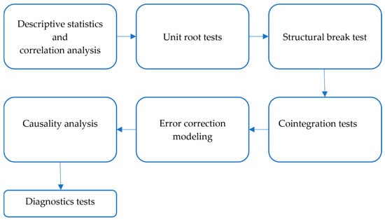
Figure 1.
Research methodology framework.
3.1. Preliminary Statistical and Econometric Analysis
To provide an initial assessment of the main characteristics of the variables, descriptive statistical indicators were calculated, including the mean, median, standard deviation, skewness, kurtosis, and the Jarque–Bera normality test. A correlation analysis was also conducted to evaluate the strength and direction of the linear relationship between interest income and non-interest income. These measures collectively describe the distributional properties, central tendencies, dispersion, and interdependence of the variables, thereby establishing a basis for the reliability of subsequent econometric analyses.
The stationarity properties of the series were examined using the Augmented Dickey–Fuller (ADF) and KPSS tests to determine the order of integration at levels and first differences. To capture smooth structural breaks and hidden cyclical components that classical tests may overlook, the Fourier KPSS test was additionally applied. The seasonal characteristics of the quarterly data were analyzed using the Hylleberg–Engle–Granger–Yoo (HEGY) test (Hylleberg et al., 1990). The optimal lag length for the ADF test was determined to be 4, based on the Modified Schwarz Criterion (MSC), whereas for the HEGY seasonal unit root test, the optimal lag length was selected as 1, according to the Akaike Information Criterion (AIC).
Potential multiple structural changes were identified through the Bai–Perron multiple structural break test (Bai & Perron, 2003), which detects break dates based on sequential F-statistics and evaluates model stability. After determining the integration order and break structure, the long-run relationships between the variables were analyzed using the Johansen cointegration test (Johansen, 1988) under various lag lengths and deterministic trends, complemented by the Fourier–ADL cointegration test, which flexibly models smooth nonlinear changes without pre-specifying breakpoints.
For cointegrated variables, a Vector Error Correction Model (VECM) was estimated to jointly capture long-run equilibrium relationships and short-run dynamics. In addition, causality patterns were examined through two complementary approaches: (i) the Fourier Toda–Yamamoto causality test, which incorporates smooth structural breaks and nonlinear adjustments into the classical framework; and (ii) the Breitung–Candelon frequency-domain causality test, which decomposes causal linkages across short-, medium-, and long-term cycles. Together, these methods provide a comprehensive view of both time-domain and frequency-specific interactions.
In the study, the methods are selected in accordance with the integration order of the variables. In Fourier analysis, the selection criteria should be clearly explained, robust tests against seasonal components should be employed, and Granger causality should be examined using alternative tests both for the overall observation period and across different frequencies. If we denote the existence of unit root in the variable at frequency ω as , then and are considered integrated at frequency ω, if , , and there exists an such that with . Full cointegration between and is possible when, for such data, for all ω (for example, for quarterly data, ω = 0, ±, π). For quarterly data, the annual difference operator can be expressed as where . The requirement of taking annual differences to render the data stationery is equivalent to the condition that the unit roots are located at . The first root corresponds to non-stationary fluctuations at zero frequency; the second root represents semi-annual or bi-annual cycles, while and correspond to annual cycles. For this purpose, the seasonal cointegration analysis proposed by Johansen and Schaumburg (1999) and the P-ME-1, P-ME-2, S-SE, S-ME-1, S-ME-2, S-ME-3 tests (Löf & Franses, 2001), the Osborn-Chui-Smith-Birchenhal (OCSB) seasonal unit root test (Osborn et al., 1999), and HEGY seasonal unit root test can be applied to identify whether seasonal oscillatory time series are stationary or non-stationary.
3.2. Justification for Fourier Methods
Fourier methods were selected because bank income structures exhibit cyclical patterns, smooth structural breaks, and nonlinear trends driven by regulatory reforms, macroeconomic shocks, and evolving market conditions. Unlike classical techniques, Fourier approaches flexibly approximate these dynamics, resulting in more reliable statistical inference and improved forecasting performance.
A detailed explanation of the Fourier techniques and their software implementation has been moved to Appendix G to streamline Section 3.
The selection of Fourier functions was carried out in accordance with the approach of Banerjee et al. (2017). The F-test and bootstrap results showed that the most appropriate frequencies are represented by the functions COS(2π·1·t/T) and SIN(2π·2·t/T). This choice can be justified both statistically (lower Akaike Information Criterion (AIC) and Schwarz Criterion (SC), improvement of diagnostic tests) and economically: COS(0.1795t) captures longer-term waves, while SIN(0.359t) models shorter-term cyclical fluctuations. Thus, the simultaneous inclusion of both components optimized the model specification.
4. Results and Discussion
Our study covers the period from the first quarter of 2016 to the third quarter of 2024, focusing on quarterly indicators (with the limitation that quarterly data may not fully capture intra-quarter fluctuations), and conducts a cointegration analysis of the interaction between interest and noninterest income (measured in millions of Azerbaijani manats). During this period, significant economic events and policy changes occurred in Azerbaijan that could have influenced the capital and foreign exchange markets.
Over the analyzed period, notable structural changes are observed in Azer Turk Bank’s interest and noninterest income, which coincide with major developments in Azerbaijan’s macroeconomic and banking sectors. Around 2017, a sharp increase in noninterest income was recorded, explained by the bank’s shift toward service-based revenue models following the dual devaluations of 2015. During that time, narrowing interest margins led banks to diversify their income sources. In 2018–2021, both income components exhibited stagnation and volatility, coinciding with macroeconomic stabilization and the global impacts of the COVID-19 pandemic, which weakened the growth of interest and service income. By contrast, in late 2022, interest income increased significantly, driven by post-pandemic recovery and the expansion of lending to small- and medium-sized enterprises (SMEs). From early 2023 to the third quarter of 2024, both types of income accelerated markedly, associated with intensified banking activity, digitalization initiatives, regulatory changes, and state-supported financing programs.
These structural shifts justify the application of Fourier cointegration and VECM models, as they reveal that the bank’s income structures are time-varying, nonlinear, and cyclical in nature. Figure 2 illustrates the dynamics of interest and noninterest income together, highlighting both linear and polynomial trends over the sample period.
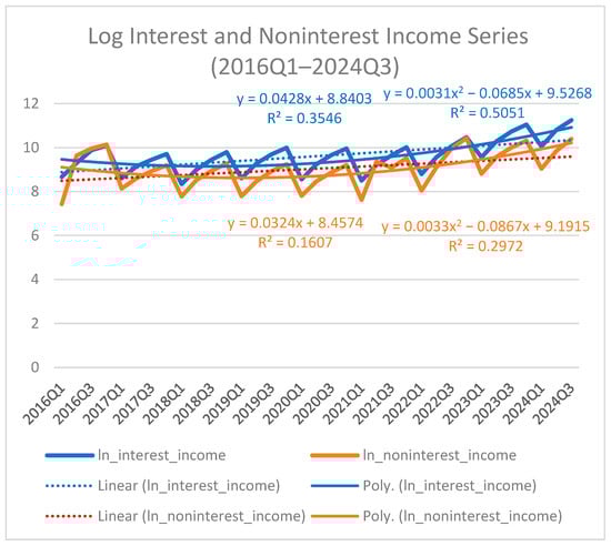
Figure 2.
Log Interest and Noninterest Income Series (2016Q1–2024Q3).
The figure presents logarithmic interest and noninterest income with fitted linear and polynomial trends. Lines correspond to fitted linear and polynomial trends.
The main variables used in the study—interest income and noninterest income—are presented in natural logarithmic form, and their descriptive statistics are reported in Table 1.

Table 1.
Descriptive statistics for the logarithms of interest and noninterest income variables.
The results of the descriptive statistics indicate that both interest income and noninterest income approximately follow a normal distribution. The closeness of the mean and median values reflects a balanced distribution without strong distortions. Skewness values close to zero reveal only slight asymmetry, while kurtosis values below three indicate flatter tails compared to the normal distribution, implying that sharp fluctuations are rare. The Jarque–Bera test confirms normality for both series at the 5% significance level.
From an economic perspective, this statistical stability shows that the income streams of Azer Turk Bank are relatively steady and not dominated by irregular jumps, thereby providing a reliable basis for econometric modeling and ensuring that subsequent cointegration and causality analyses are not distorted by excessive volatility. The correlation coefficient between the variables is = 0.91, confirming a strong positive linear relationship between interest and noninterest income. The high degree of correlation demonstrates that the variables move in the same direction and synchronously, as well as the presence of common macroeconomic determinants shaping them. This finding provides a solid statistical foundation for evaluating cointegration relationships and strengthens the likelihood of a long-term equilibrium link.
To evaluate the stationarity properties of the time series and to determine the order of integration, ADF and KPSS unit root tests were conducted under two specifications: with intercept only and with intercept + trend. The Modified Schwarz Criterion (MSC) was chosen because our sample is relatively small (35 quarters). MSC applies a stricter penalty on extra lags, preventing overfitting and yielding more parsimonious and robust models. This makes MSC the most reliable criterion for our analysis. The ADF test results (see Table A1 in Appendix A) indicate that the interest income and noninterest income series are non-stationary in levels but become stationary after first differencing, confirming that both variables are integrated of order one, I(1). Similarly, the KPSS test results (see Table A2 in Appendix A) show non-stationarity in levels and stationarity at first differences.
To account for the seasonal nature of the quarterly data, the HEGY test was employed. For each frequency, the test statistics were compared against the 1%, 5%, and 10% critical values reported in Table A3 in Appendix A. The results reveal that both series contain unit roots at the 0 frequency (non-seasonal component), while no unit roots are detected at the seasonal frequencies (π/2 and 3π/2), and the π frequency is not statistically significant. Accordingly, the cointegration analysis focuses on the 0 frequency, which is standard practice in the literature for examining long-run equilibrium relationships.
Finally, the Fourier KPSS results (see Table A4 in Appendix A) are considered. Unlike the traditional KPSS test, this approach employs trigonometric Fourier functions to more effectively capture nonlinear deterministic components and potential structural breaks. The Fourier KPSS test results indicate that both interest income and noninterest income are non-stationary in levels but become stationary after first difference. The F-test results further confirm that the trigonometric functions are significant in levels but insignificant at the first order (Burjaliyeva, 2025).
The Bai–Perron multiple break test (Appendix C) showed evidence of a structural break in noninterest income. The sequential F-statistic for the comparison of no break versus one break was 16.36, which is higher than the 5% critical value of 11.47. This result confirms the presence of a break in the first quarter of 2023. Further testing for an additional break (one versus two) did not provide statistical support, indicating that only a single break occurred. From an economic perspective, this change can be linked to the post-COVID-19 period, when the banking sector experienced stronger activity, state-supported programs expanded, and SME lending intensified.
The results of the Fourier–ADL cointegration test (Appendix B) indicate the existence of a long-term relationship between interest and noninterest income; however, the strength of this relationship varies depending on the significance level. Since the test accounts for smooth structural breaks, confirmation at the 1% level would have provided very strong evidence. Nevertheless, cointegration is confirmed only at the 5% and 10% levels, suggesting moderate rather than strong stability. The key advantage of the Fourier–ADL approach is that it detects cointegration without requiring predefined break dates and better captures cyclical components than classical methods. Thus, the Fourier–ADL test supports a long-term equilibrium, but one of medium strength. It should also be noted that sine and cosine functions were not simultaneously significant across all frequencies. In some cases, only the sine function was significant, while in others, only the cosine function proved significant; therefore, their inclusion as exogenous variables was guided by model selection criteria.
Table 2 presents the results of the Johansen cointegration test, which further confirms the existence of a long-term equilibrium relationship between interest and noninterest income. In this analysis, the Fourier functions SIN(0.359t) and COS(0.1795t) were included as exogenous variables.
Table 2.
Johansen cointegration results with Fourier functions for interest and noninterest income.
The results of the Trace and Maximum Eigenvalue statistics indicate the existence of one cointegrating vector across all deterministic trend specifications. According to the AIC and SC criteria, the most optimal specification is identified as the linear trend with one cointegrating vector (AIC = 1.142, SC = 1.829).
The results of the Johansen test confirm the existence of one cointegrating vector across all specifications, with the best-fitting model determined as the linear trend with one vector. This strongly demonstrates the presence of a stable long-term relationship between interest and noninterest income. The inclusion of Fourier functions captures cyclical dynamics, thereby extending earlier studies that relied solely on linear cointegration approaches. These findings are also consistent with Pascalau et al. (2022), who emphasized the importance of incorporating Fourier functions into cointegration tests to achieve more reliable results in the presence of structural breaks.
Overall, these results demonstrate the existence of a statistically significant and stable long-term relationship between interest and noninterest income. Moreover, this relationship is characterized by intertemporal structural stability over the analyzed period. The inclusion of Fourier functions further justifies the necessity of accounting for cyclical and nonlinear dynamics within the system. Consequently, the resulting VECM incorporates these elements and is specified as follows:
Here,, ( represents the lagged values of the respective variable. The adjustment coefficients,, are statistically significant. This implies that interest income tends to correct deviations from the long-term equilibrium that occurred in the previous period and directs the system back toward its stable state. In response to shocks affecting the explanatory variables in earlier periods, deviations of the dependent variables from their equilibrium levels are corrected within approximately , respectively—that is, about . The adjustment speeds indicated by the magnitudes of the adjustment coefficients confirm the existence of a mean-reverting mechanism and empirically demonstrate that the system tends to restore long-term equilibrium after temporary disturbances.
For Equation (1), the long-run equilibrium dependence is expressed as:
The short-run effects of changes are determined by the sum of the lagged difference variables as follows:
The cyclical fluctuations are defined by the expression The influence of each of these lagged difference variables on the current values of the differenced operators is inelastic. The same procedure is applied for the calculations concerning noninterest income.
The VECM results indicate that when both income streams deviate from long-term equilibrium, a short-run adjustment mechanism is activated. In particular, the negative and statistically significant cointegration vectors show that both interest and noninterest income reduce deviations from equilibrium and guide the system back toward stability.
The details of the short-run dynamics reveal a more nuanced picture. The lags of interest income generally appear with negative coefficients, indicating that increases in the previous period are followed by declines in the subsequent period. At the same time, the positive and strong effect at the fourth lag suggests the formation of a restorative wave after a certain period. The consistent positive effect of past noninterest income values on interest income further confirms the mutually reinforcing relationship between income components.
On the other hand, the dynamics of noninterest income are weaker. Here, the primary role is played by the past values of interest income, whose positive influence stimulates noninterest income in the short run. This finding suggests that interest income plays a leading role in banking activity, while noninterest income behaves more reactively.
The Fourier functions included in the model highlight the cyclical nature of incomes. The negative significance of the sine function and the positive and strong significance of the cosine function imply that the observed variations are not solely driven by trend and random shocks but are also characterized by periodic fluctuations. This result confirms the important role of cyclical factors in the short-term development of bank income.
Appendix E presents the estimated Fourier A (cosine) and B (sine) coefficients used in the Fourier–ADL and Fourier–VECM models. The statistical significance of these coefficients indicates that smooth cyclical components are present in both interest and non-interest income dynamics. These results justify the inclusion of Fourier functions, as they capture medium- and long-run nonlinear adjustments that cannot be explained by standard deterministic trends.
Appendix F illustrates the estimated Fourier A (cosine) and B (sine) components for both income measures. These figures visualize the cyclical dynamics captured by the Fourier functions, highlighting smooth oscillations around the deterministic trend that justify the use of Fourier-based cointegration models.
The results of the application of the Fourier Toda–Yamamoto approach are presented in Table 3. This approach extends the traditional Toda–Yamamoto test by incorporating smooth structural breaks and cyclical dynamics, thereby enabling a more precise identification of causality relationships in time series, such as bank incomes, which are affected by nonlinear and seasonal influences.
Table 3.
Fourier Toda–Yamamoto causality results between interest and noninterest income.
The results of this table correspond to the Fourier Toda–Yamamoto causality test and demonstrate the directionality between interest income and noninterest income. According to the findings, causality from interest income to noninterest income is very strong and statistically significant (χ2 = 88.87; p < 0.001). This implies that changes in interest income directly influence both the short- and long-term dynamics of noninterest income. In the reverse direction, the effect from noninterest income to interest income is only marginally significant (χ2 = 8.99; p ≈ 0.06). This suggests that while noninterest income may exert some influence on interest income, this effect is neither strong nor stable.
Overall, the results confirm that interest income plays a leading role in the structure of bank revenues, whereas noninterest income remains more dependent and reactive in nature. This also provides practical implications for income diversification strategies in the sector: the growth of noninterest income is often shaped as a continuation or derivative of movements in interest income.
In this test, the choice of lag length p = 4 and integration order d = 1 is justified not only technically but also theoretically and empirically. Since the data are quarterly, four lags cover one annual seasonal cycle and allow for the proper capture of intra-annual cyclical variations observed in bank income dynamics. Moreover, an extensive grid search indicated that the lowest values of the AIC and BIC information criteria are consistently achieved with four lags. This enhances the model’s goodness of fit while avoiding unnecessary parameter inflation, thereby ensuring a parsimonious specification.
Furthermore, the Lagrange Multiplier (LM) serial correlation tests and the Durbin–Watson statistic, which is close to 2, confirm the absence of autocorrelation in the residuals. This strengthens the validity of choosing p = 4 from both a statistical stability and an economic interpretation perspective. Regarding the order of integration, the results of the ADF/KPSS tests clearly show that both interest and noninterest income are non-stationary in levels but stationary in first differences (I(1)). This theoretically validates the precondition for cointegration. The findings are also consistent with the results of the Johansen and Fourier–ADL cointegration tests, confirming that the variables share a stable long-term equilibrium relationship.
Table 4 reports the results of the frequency-domain Granger causality test, which evaluates causality relationships between interest and noninterest income across different frequencies.
Table 4.
Spectral Granger Causality Test Results.
The results indicate that at low and medium frequencies, causality running from interest income to noninterest income is stronger and statistically significant. This suggests that changes in interest income generate cyclical and persistent effects on noninterest income.
Conversely, causality from noninterest income to interest income is weaker and attains only marginal significance at very low frequencies (e.g., 0.18 radians). At higher frequencies, the effect from interest income to noninterest income remains consistently strong (p < 0.01), whereas the reverse effect is virtually absent.
In sum, the causality tests confirm the asymmetric relationship: interest income consistently drives noninterest income over short- and medium-term horizons, while the reverse effect is weak. This result aligns with Burjaliyeva (2025) in the Azerbaijani context but contrasts with Abu Khalaf et al. (2024), who found that noninterest income plays a stabilizing role in MENA banks.
Various diagnostic tests were conducted to assess the adequacy of the VECM specification. First, the LM tests (Appendix D.1 and Appendix D.2) indicate that no serial autocorrelation exists in the residuals.
The normality tests (Appendix D.3) present a more mixed picture. While the residuals of the first component are close to a normal distribution (p ≈ 0.91, p ≈ 0.30), the skewness and kurtosis statistics for the second component are significant. The joint Jarque–Bera statistic rejects the null hypothesis at p = 0.007, indicating some non-normality in the residual distribution (asymmetry and fat tails). Nevertheless, such deviations from normality are common in Fourier-type models and do not substantially weaken the interpretation of the results.
Heteroskedasticity tests (Appendix D.4) confirm the assumption of constant variance. The joint test yields a p-value of 0.64, failing to reject the null hypothesis of homoskedasticity. This demonstrates that the residuals possess constant variance and that heteroskedasticity is not a serious concern in the model.
Finally, the Ramsey Regression Equation Specification Error Test (RESET) tests (Appendix D.5) were applied to check the correctness of the specification. In both specifications, the main F-tests are insignificant, indicating that no additional nonlinear terms are required. This confirms that the functional form of the model is well specified.
Overall, all diagnostic checks (Appendix D.1, Appendix D.2, Appendix D.3, Appendix D.4 and Appendix D.5) verify that the specification of the Fourier-based VECM is adequate and that the results can be interpreted with confidence in terms of stability and forecasting accuracy.
5. Conclusions
This study empirically demonstrates the existence of a stable long-term relationship between interest and noninterest income at Azer Turk Bank and reveals asymmetric dynamics in the short and medium term. The results of the ADF, KPSS, and Fourier–KPSS tests consistently indicate that both interest and noninterest income series are non-stationary in levels but become stationary after first differencing, implying integration of order one, I(1). The Hylleberg–Engle–Granger–Yoo (HEGY) seasonal unit root test provides complementary evidence, confirming the presence of a unit root at the non-seasonal (0) frequency for both series, while no unit roots are detected at the seasonal frequencies (π/2 and 3π/2). This finding demonstrates that non-stationarity arises from long-term stochastic trends rather than seasonal components. Johansen and Fourier–ADL tests support the presence of cointegration. The results of the Fourier-based VECM clearly confirm the mean-reverting mechanism, showing that deviations from equilibrium are corrected within approximately 5.9; 2.5 quarters. The Fourier Toda–Yamamoto and frequency-domain Granger tests indicate consistent and statistically strong causality running from interest income to noninterest income, while the reverse effect remains weak or insignificant. This finding highlights that noninterest income is still highly dependent on the credit cycle and interest margins, suggesting that its diversification potential remains limited.
By integrating Fourier functions into the VECM framework with explicit mathematical expressions, the study offers a practical Fourier-VECM approach to model cyclical deviations around smooth breaks and nonlinear trends. Compared to classical linear approaches, this framework captures cyclical components more adequately, thereby improving diagnostics and forecasting accuracy. Diagnostic checks, including RESET, LM, heteroskedasticity, and stability tests, confirm the reliability of the specification.
The findings yield clear policy implications. For banks, the development of commission-based and digital services is essential to reduce sensitivity to credit cycles and interest rate volatility. For regulators, the application of Fourier-based methods can enhance risk assessment, stress testing, and the design of macroprudential policies, thereby strengthening compliance with Basel III requirements and improving system stability. For policymakers, Fourier-based models provide the ability to detect cyclical vulnerabilities earlier than traditional methods, reinforcing macroprudential supervision.
Future research should extend the application of Fourier-VECM models to multiple banks and different country contexts. Such approaches would clarify whether the observed asymmetric dependencies are unique to Azer Turk Bank or reflect broader vulnerabilities in emerging banking systems, offering valuable guidance for comparative stress-testing exercises by regulators.
6. Limitations
This study is subject to several limitations. First, the dataset is based solely on the quarterly financial reports of Azer Turk Bank over the past decade (2016Q1–2024Q3). As a result, the number of observations is limited, which may somewhat weaken the statistical power of the results.
Second, the analysis focuses exclusively on a single bank—Azer Turk Bank. This constrains the generalizability of the findings to the entire banking sector, as ATB’s partial state ownership, strategic orientation toward SMEs, and specific business model may differ from those of other banks.
Third, while the application of Fourier functions is useful for capturing cyclical dynamics and smooth structural breaks, it does not fully reflect the impacts of sudden economic events (e.g., the 2015 devaluation, the COVID-19 pandemic). To this end, the Bai–Perron multiple break test indicated the presence of a structural break in noninterest income in 2023Q1. Nevertheless, the incomplete modeling of abrupt breaks under the Fourier approach remains an additional limitation.
Fourth, the models account only for interest and noninterest income, while key macroeconomic variables (such as interest rates, inflation, and regulatory policies) are excluded, even though these factors significantly influence bank income structures.
Fifth, Johansen test critical values are tabulated assuming no exogenous regressors; because our specification includes trigonometric functions, the resulting inference should be interpreted with caution.
Finally, the results of Fourier-based cointegration and causality tests are sensitive to the selected frequency parameters and lag lengths. Alternative specifications may yield different outcomes, and therefore the findings should be interpreted with appropriate caution.
Author Contributions
Conceptualization, E.G.O.; methodology, E.G.O. and N.G.B.; software, N.G.B.; validation, E.G.O. and N.G.B.; formal analysis, N.G.B.; investigation, N.G.B.; resources, N.G.B.; data curation, N.G.B.; writing—original draft preparation, N.G.B.; writing—review and editing, E.G.O. and N.G.B.; visualization, N.G.B.; supervision, E.G.O.; project administration, E.G.O. and N.G.B. All authors have read and agreed to the published version of the manuscript.
Funding
This research received no external funding.
Institutional Review Board Statement
Not applicable.
Informed Consent Statement
Not applicable.
Data Availability Statement
The data used in this study comprise interest income and non-interest income indicators, which were obtained from the publicly available financial reports of Azer Turk Bank. These reports can be accessed at the following official website: https://atb.az/financial/ (accessed on 24 November 2024). No proprietary or confidential data were used in the analysis.
Conflicts of Interest
The authors declare no conflicts of interest.
Abbreviations
The following abbreviations are used in this manuscript:
| ADF | Augmented Dickey–Fuller |
| AIC | Akaike Information Criterion |
| ARDL | Autoregressive Distributed Lag |
| BIC | Bayesian Information Criterion |
| CE/CEs | Cointegrating Equation(s) |
| CO2 | Carbon dioxide |
| DOLS | Dynamic Ordinary Least Squares |
| DW | Durbin–Watson statistic |
| ECM | Error Correction Mechanism |
| Fourier–ADL | Fourier Autoregressive Distributed Lag |
| Fourier KPSS | Fourier Kwiatkowski–Phillips–Schmidt–Shin |
| GDP | Gross Domestic Product |
| HEGY | Hylleberg–Engle–Granger–Yoo seasonal unit root test |
| IMF | International Monetary Fund |
| JB | Jarque–Bera |
| LM | Lagrange Multiplier |
| LRE* | Likelihood ratio statistic |
| MinSSR | Minimum Sum of Squared Residuals |
| OCSB | Osborn–Chui–Smith–Birchenhall unit root test |
| RESET | Ramsey Regression Equation Specification Error Test |
| SC | Schwarz Bayesian Criterion |
| SE | Standard Error |
| SMEs | Small- and Medium-sized Enterprises |
| SSR | Sum of Squared Residuals |
| VAR | Vector Autoregression |
| VECM | Vector Error Correction Model |
Appendix A. Unit Root and Stationarity Test Results
Table A1.
Classical Augmented Dickey–Fuller (ADF) test results (Modified Schwarz Criterion).
Table A1.
Classical Augmented Dickey–Fuller (ADF) test results (Modified Schwarz Criterion).
| Variable | Spec. | ADF Stat. | 1% Critical Value | 5% Critical Value | 10% Critical Value | Result |
|---|---|---|---|---|---|---|
| LN_INTEREST_INCOME | Intercept | −0.8162 | −3.6702 | −2.9640 | −2.6210 | Non-stationary |
| LN_INTEREST_INCOME | Intercept + trend | −0.7969 | −4.3098 | −3.5742 | −3.2217 | Non-stationary |
| ∆LN_INTEREST_INCOME | Intercept | −7.7865 | −3.6463 | −2.9540 | −2.6158 | Stationary |
| ∆LN_INTEREST_INCOME | Intercept + trend | −7.7123 | −4.2627 | −3.5530 | −3.2096 | Stationary |
| LN_NONINTEREST_INCOME | Intercept | −0.4753 | −3.6702 | −2.9640 | −2.6210 | Non-stationary |
| LN_NONINTEREST_INCOME | Intercept + trend | −1.7950 | −4.3240 | −3.5806 | −3.2253 | Non-stationary |
| ∆LN_NONINTEREST_INCOME | Intercept | −8.3601 | −3.6463 | −2.9540 | −2.6158 | Stationary |
| ∆LN_NONINTEREST_INCOME | Intercept + trend | −8.2380 | −4.2627 | −3.5530 | −3.2096 | Stationary |
Table A2.
Kwiatkowski–Phillips–Schmidt–Shin (KPSS) test results.
Table A2.
Kwiatkowski–Phillips–Schmidt–Shin (KPSS) test results.
| Variable | Spec. | KPSS Stat. | 1% Crit. Value | 5% Crit. Value | 10% Crit. Value | Result |
|---|---|---|---|---|---|---|
| LN_INTEREST_INCOME | Intercept | 0.5906 | 0.739 | 0.463 | 0.347 | Not stationary (5%) |
| LN_INTEREST_INCOME | Intercept + trend | 0.2293 | 0.216 | 0.146 | 0.119 | Not stationary (1%) |
| ∆LN_INTEREST_INCOME | Intercept | 0.1857 | 0.739 | 0.463 | 0.347 | Stationary |
| ∆LN_INTEREST_INCOME | Intercept + trend | 0.1857 | 0.216 | 0.146 | 0.119 | Stationary |
| LN_NONINTEREST_INCOME | Intercept | 0.5854 | 0.739 | 0.463 | 0.347 | Not stationary (5%) |
| LN_NONINTEREST_INCOME | Intercept + trend | 0.1646 | 0.216 | 0.146 | 0.119 | Not stationary (5%) |
| ∆LN_NONINTEREST_INCOME | Intercept | 0.2193 | 0.739 | 0.463 | 0.347 | Stationary |
| ∆LN_NONINTEREST_INCOME | Intercept + trend | 0.2141 | 0.216 | 0.146 | 0.119 | Stationary |
Table A3.
Hylleberg–Engle–Granger–Yoo (HEGY) Test Results.
Table A3.
Hylleberg–Engle–Granger–Yoo (HEGY) Test Results.
| Variable | Frequency | Test Stat. | 1% Crit. | 5% Crit. | 10% Crit. | Stationary |
|---|---|---|---|---|---|---|
| LN_INTEREST_INCOME | 0 | –1.164 | –3.65 | –3.12 | –2.85 | No |
| LN_INTEREST_INCOME | π/2 & 3π/2 | 3.560 | 2.79 | 1.19 | 0.75 | Yes |
| LN_INTEREST_INCOME | π | –1.350 | –3.26 | –2.71 | –2.42 | No |
| LN_INTEREST_INCOME | All | 3.537 | 5.77 | 4.15 | 3.43 | No |
| LN_NONINTEREST_INCOME | 0 | –2.081 | –3.65 | –3.12 | –2.85 | No |
| LN_NONINTEREST_INCOME | π/2 & 3π/2 | 9.911 | 2.79 | 1.19 | 0.75 | Yes |
| LN_NONINTEREST_INCOME | π | –2.566 | –3.26 | –2.71 | –2.42 | Weak |
| LN_NONINTEREST_INCOME | All | 14.280 | 5.77 | 4.15 | 3.43 | Yes |
Note: The 0 frequency corresponds to the non-seasonal component, π/2 and 3π/2 represent seasonal frequencies in quarterly data, and π corresponds to semiannual periodicity.
Table A4.
Fourier KPSS results.
Table A4.
Fourier KPSS results.
| Variable | Frequency | MinSSR | FKPSS | F-Test Statistics |
|---|---|---|---|---|
| ln(interest income) | 1 | 13.17047 | 0.27653 | 6.42837 |
| ln(noninterest income) | 1 | 17.16470 | 0.22873 | 5.70625 |
| d(ln(interest income)) | 1 | 20.51771 | 0.088 | 0.0762 |
| d(ln(noninterest income)) | 4 | 37.43692 | 0.17105 | 0.12244 |
Note: For T = 100, the F-statistics level critical values are 4.133, 4.929, and 6.730 at the 10%, 5%, and 1% significance levels, respectively. The critical values for the Fourier KPSS test statistic are as follows: for k = 1, 0.1318, 0.1720, and 0.2699; and for k = 4, 0.3476, 0.4592, and 0.7222 at the 10%, 5%, and 1% significance levels, respectively. (Reproduced from Burjaliyeva, 2025, with author’s permission. The test statistics and F-values were taken from the authors’ previous study, while the critical values were reproduced from Becker et al. (2006)).
Appendix B. Fourier–ADL
Table A5.
Fourier–ADL (Banerjee et al., 2017) estimation summary for ΔLN_NONINTEREST_INCOME with SIN(kωt), COS(kωt).
Table A5.
Fourier–ADL (Banerjee et al., 2017) estimation summary for ΔLN_NONINTEREST_INCOME with SIN(kωt), COS(kωt).
| k | Selection | Lags (Δy, Δx) | Adj. R2 | SEE | DW | SIN(kωt) | COS(kωt) | xt−1 |
|---|---|---|---|---|---|---|---|---|
| 1 | AIC | (4, 1) | 0.939 | 0.229 | 2.19 | −0.192 (**) | −0.099 | 0.092 |
| 1 | BIC | (4, 1) | 0.939 | 0.229 | 2.19 | −0.192 (**) | −0.099 | 0.092 |
| 2 | AIC | (6, 4) | 0.940 | 0.235 | 2.45 | +0.382 (**) | −0.096 | −0.448 |
| 2 | BIC | (1, 1) | 0.922 | 0.267 | 2.08 | +0.035 | +0.021 | −0.053 |
| 3 | AIC | (3, 1) | 0.924 | 0.272 | 2.20 | +0.035 | +0.055 | +0.028 |
| 3 | BIC | (1, 1) | 0.923 | 0.266 | 2.12 | −0.020 | +0.047 | −0.062 |
Note: Dependent variable: Δyt; regressors include SIN, COS, yt−1, xt−1, Δx and lags, Δyt and lags. Stars (**) indicate statistical significance at the 5% level. AIC = Akaike Information Criterion; BIC = Bayesian Information Criterion; DW = Durbin–Watson statistic.
Appendix C. Bai–Perron Multiple Breakpoint Test
Table A6.
Sequential F-statistics for L + 1 vs. L breaks (trimming 0.15; max breaks 5; α = 0.05).
Table A6.
Sequential F-statistics for L + 1 vs. L breaks (trimming 0.15; max breaks 5; α = 0.05).
| Null Hypothesis | Alternative Hypothesis | F-Stat. | Scaled F-Stat. | 5% Critical Value | Decision |
|---|---|---|---|---|---|
| 0 breaks | 1 break | 16.36914 * | 32.73828 | 11.47 | Reject H0 → 1 break |
| 1 break | 2 breaks | 5.394812 | 10.78962 | 12.95 | Fail to reject H0 |
Note: Break date (sequential & repartition): 2023Q1. The asterisk (*) denotes statistical significance at the 5% level.
Appendix D. Diagnostic Tests
Appendix D.1
Table A7.
Vector Error Correction (VEC) residual serial correlation Lagrange Multiplier (LM) tests (individual lag h).
Table A7.
Vector Error Correction (VEC) residual serial correlation Lagrange Multiplier (LM) tests (individual lag h).
| Lag | LRE* Stat | df | p-Value | Rao F-Stat | df | p-Value |
|---|---|---|---|---|---|---|
| 1 | 5.559515 | 4 | 0.2345 | 1.473199 | (4, 30.0) | 0.2350 |
| 2 | 3.201760 | 4 | 0.5246 | 0.816035 | (4, 30.0) | 0.5251 |
| 3 | 1.018213 | 4 | 0.9070 | 0.250432 | (4, 30.0) | 0.9071 |
| 4 | 4.763181 | 4 | 0.3125 | 1.245629 | (4, 30.0) | 0.3130 |
| 5 | 5.662995 | 4 | 0.2258 | 1.503202 | (4, 30.0) | 0.2262 |
Note: LRE* = Edgeworth expansion–corrected likelihood ratio statistic.
Appendix D.2
Table A8.
VEC Residual Serial Correlation LM Tests (cumulative, lags 1 … h).
Table A8.
VEC Residual Serial Correlation LM Tests (cumulative, lags 1 … h).
| Lag (1 … h) | LRE* Stat | df | p-Value | Rao F-Stat | df | p-Value |
|---|---|---|---|---|---|---|
| 1 | 5.559515 | 4 | 0.2345 | 1.473199 | (8, 26.0) | 0.3899 |
| 2 | 8.506270 | 8 | 0.3856 | 1.107832 | (8, 26.0) | 0.3899 |
| 3 | 10.21920 | 12 | 0.5967 | 0.843474 | (12, 22.0) | 0.6092 |
| 4 | 15.97552 | 16 | 0.4547 | 1.006453 | (16, 18.0) | 0.4910 |
| 5 | 23.05630 | 20 | 0.2860 | 1.207460 | (20, 14.0) | 0.3649 |
Note: LRE* = Edgeworth expansion–corrected likelihood ratio statistic.
Appendix D.3
Table A9.
VEC Residual Normality Tests (Cholesky orthogonalization).
Table A9.
VEC Residual Normality Tests (Cholesky orthogonalization).
| Component | Skewness | Chi-sq | df | p-Value |
| 1 | −0.049639 | 0.012320 | 1 | 0.9116 |
| 2 | 1.145685 | 6.562972 | 1 | 0.0104 |
| Joint | — | 6.575292 | 2 | 0.0373 |
| Component | Kurtosis | Chi-sq | df | p-Value |
| 1 | 4.381816 | 2.386769 | 1 | 0.1224 |
| 2 | 5.004097 | 5.020508 | 1 | 0.0250 |
| Joint | — | 7.407276 | 2 | 0.0246 |
| Component | JB | df | p-Value | |
| 1 | 2.399089 | 2 | 0.3013 | |
| 2 | 11.58348 | 2 | 0.0031 | |
| Joint | 13.98257 | 4 | 0.0074 | |
Note: JB = Jarque–Bera normality test.
Appendix D.4
Table A10.
VEC Residual Heteroskedasticity Tests (levels & squares).
Table A10.
VEC Residual Heteroskedasticity Tests (levels & squares).
| Chi-sq | df | p-Value | |||
| 61.26963 | 66 | 0.6419 | |||
| Individual Components | |||||
| Dependent | R-Squared | F(22, 7) | p-Value | Chi-sq(22) | p-Value |
| res1×res1 | 0.850636 | 1.812057 | 0.2140 | 25.51907 | 0.2729 |
| res2×res2 | 0.818427 | 1.434185 | 0.3260 | 24.55282 | 0.3189 |
| res2×res1 | 0.399600 | 0.211768 | 0.9977 | 11.98800 | 0.9576 |
Appendix D.5
Table A11.
Ramsey Regression Equation Specification Error Test (RESET)—VECM.
Table A11.
Ramsey Regression Equation Specification Error Test (RESET)—VECM.
| Statistic | Value | df | p-Value |
|---|---|---|---|
| t-statistic | 0.539947 | 23 | 0.5944 |
| F-statistic | 0.291543 | (1, 23) | 0.5944 |
| Likelihood ratio | 0.415672 | 1 | 0.5191 |
Appendix E. Spectral Density and Fourier Coefficient Estimates
Appendix E.1
Table A12.
Spectral Density and Fourier Coefficient Estimates of the LN_INTEREST_INCOME Series.
Table A12.
Spectral Density and Fourier Coefficient Estimates of the LN_INTEREST_INCOME Series.
| Angular Frequency (Omega) | Frequency (Cycle/Time Unit) | Cycle Frequency (Time Unit/Cycle) | Periodogram | Estimated A | Estimated B |
|---|---|---|---|---|---|
| 0.179520 | 0.028571 | 35.00000 | 0.549885 | 0.423701 | −0.350502 |
| 0.359039 | 0.057143 | 17.50000 | 0.359626 | 0.197220 | −0.300724 |
| 0.538559 | 0.085714 | 11.66667 | 0.103097 | −0.009194 | −0.102686 |
| 0.718078 | 0.114286 | 8.750000 | 0.108050 | −0.024854 | −0.105152 |
| 0.897598 | 0.142857 | 7.000000 | 0.094366 | 0.001499 | −0.094354 |
| 1.077117 | 0.171429 | 5.833333 | 0.072529 | −0.011831 | −0.071557 |
| 1.256637 | 0.200000 | 5.000000 | 0.100626 | −0.018171 | −0.098972 |
| 1.436157 | 0.228571 | 4.375000 | 0.160673 | −0.149857 | −0.057954 |
| 1.615676 | 0.257143 | 3.888889 | 0.614972 | 0.583360 | −0.194633 |
| 1.795196 | 0.285714 | 3.500000 | 0.149372 | 0.128901 | −0.075476 |
| 1.974715 | 0.314286 | 3.181818 | 0.118263 | 0.109944 | −0.043570 |
| 2.154235 | 0.342857 | 2.916667 | 0.098270 | 0.084251 | −0.050583 |
| 2.333755 | 0.371429 | 2.692308 | 0.092017 | 0.077417 | −0.049737 |
| 2.513274 | 0.400000 | 2.500000 | 0.075780 | 0.060229 | −0.045990 |
| 2.692794 | 0.428571 | 2.333333 | 0.079592 | 0.047806 | −0.063635 |
| 2.872313 | 0.457143 | 2.187500 | 0.106972 | 0.066521 | −0.083773 |
| 3.051833 | 0.485714 | 2.058824 | 0.307773 | 0.069183 | −0.299896 |
Appendix E.2
Table A13.
Spectral Density and Fourier Coefficient Estimates of the LN_NONINTEREST_INCOME Series.
Table A13.
Spectral Density and Fourier Coefficient Estimates of the LN_NONINTEREST_INCOME Series.
| Angular Frequency (Omega) | Frequency (Cycle/Time Unit) | Cycle Frequency (Time Unit/Cycle) | Periodogram | Estimated A | Estimated B |
|---|---|---|---|---|---|
| 0.179520 | 0.028571 | 35.00000 | 0.591445 | 0.492611 | −0.327325 |
| 0.359039 | 0.057143 | 17.50000 | 0.133788 | 0.036757 | −0.128639 |
| 0.538559 | 0.085714 | 11.66667 | 0.065903 | −0.046901 | 0.046298 |
| 0.718078 | 0.114286 | 8.750000 | 0.116715 | −0.110976 | 0.036147 |
| 0.897598 | 0.142857 | 7.000000 | 0.073684 | −0.068285 | −0.027685 |
| 1.077117 | 0.171429 | 5.833333 | 0.207231 | −0.093054 | −0.185164 |
| 1.256637 | 0.200000 | 5.000000 | 0.210921 | −0.190003 | −0.091576 |
| 1.436157 | 0.228571 | 4.375000 | 0.168053 | −0.162859 | −0.041458 |
| 1.615676 | 0.257143 | 3.888889 | 0.685160 | 0.624704 | −0.281407 |
| 1.795196 | 0.285714 | 3.500000 | 0.173259 | 0.132546 | −0.111581 |
| 1.974715 | 0.314286 | 3.181818 | 0.189303 | 0.135259 | −0.132442 |
| 2.154235 | 0.342857 | 2.916667 | 0.116263 | 0.039565 | −0.109324 |
| 2.333755 | 0.371429 | 2.692308 | 0.117295 | 0.106126 | −0.049954 |
| 2.513274 | 0.400000 | 2.500000 | 0.195864 | 0.121501 | −0.153623 |
| 2.692794 | 0.428571 | 2.333333 | 0.106153 | 0.062391 | −0.085883 |
| 2.872313 | 0.457143 | 2.187500 | 0.216423 | 0.174733 | −0.127700 |
| 3.051833 | 0.485714 | 2.058824 | 0.405989 | 0.098495 | −0.393860 |
Appendix F. Fourier Approximation Components of the Series
In the context of the Fourier approximation, the A component corresponds to the cosine coefficient, while the B component corresponds to the sine coefficient, capturing the cyclical behavior of the series at the selected frequency.

Figure A1.
A component on LN_INTEREST_INCOME.
Figure A1.
A component on LN_INTEREST_INCOME.


Figure A2.
B component on LN_INTEREST_INCOME.
Figure A2.
B component on LN_INTEREST_INCOME.


Figure A3.
A component on LN_NONINTEREST_INCOME.
Figure A3.
A component on LN_NONINTEREST_INCOME.


Figure A4.
B component on LN_NONINTEREST_INCOME.
Figure A4.
B component on LN_NONINTEREST_INCOME.

Appendix G. Mathematical Formulation and Implementation of Fourier-Based Econometric Tests
This appendix provides the detailed mathematical formulation and implementation steps for the Fourier KPSS, Fourier–ADL, Fourier Toda–Yamamoto, and Breitung–Candelon frequency-domain causality tests. All econometric analyses were performed in EViews 12 and WinRATS Pro 10, following the procedures described in Becker et al. (2006), Banerjee et al. (2017), and Breitung and Candelon (2006).
All tests and models were implemented in EViews 12 and WinRATS Pro 10 (Hepsağ, 2022). To ensure the robustness of the results, several diagnostic checks were carried out, including the Durbin–Watson statistic and the LM test for serial correlation, residual test for heteroskedasticity, the Jarque–Bera test for residual normality, the Ramsey RESET test for functional form misspecification, and the Bai–Perron multiple break test for structural stability.
The frequency-domain Granger causality test extends this framework by decomposing the relationship between variables and across different frequency bands. This approach allows for the evaluation of causality at specific frequencies ω, thereby distinguishing short-, medium-, and long-term dynamics.
Here, for the bivariate time series , :
(, —white noise, E( = 0, E(’) = , positive definite), if is a lower triangular matrix satisfying = and E(, , and the system is assumed stationary, then the MA representation is:
Here, and . Using (A1), the spectral density of can be expressed as:
The causality measure is defined as:
This measure equals zero when = 0. In this case, does not cause at frequency . By separating the left-hand side into real and imaginary parts,
which yields the equivalent conditions:
At and , . For
The relation is equivalent to
Here
For the null hypothesis , the usual F-statistic is approximately distributed as for .
Consequently, the null hypothesis in the frequency domain is formulated as follows:
Here, the indicator My→x represents the measure of causality from to at a specific frequency ω. The frequency-domain causality test transforms the coefficients of a standard Vector Autoregression (VAR) model into a spectral representation, allowing causality to be evaluated across different cyclical horizons.
Stationarity is tested using the Fourier KPSS test, which represents an extended version of the stationarity test originally proposed by Kwiatkowski, Phillips, Schmidt, and Shin (KPSS). The regression model used for this test is specified as follows:
Here, denotes the number of frequencies considered in the model, represents the partial frequency, refers to the total number of observations, and indicates the deterministic trend. In the special case where , the model simplifies to a form that includes only an intercept. This formulation enables the Fourier KPSS test to effectively account for structural breaks and nonlinear trends present in time series. As a result, the robustness of the test during the stationarity assessment is significantly enhanced, and more accurate results can be obtained even in the presence of structural changes.
Here, and represent the coefficients of the Fourier functions. The test statistic for stationarity is calculated using Equation (A10):
In the Fourier KPSS test, the null hypothesis assumes that the time series is stationary () and is tested against the alternative hypothesis. If the Fourier KPSS test statistic is smaller than the critical values, the null hypothesis cannot be rejected (i.e., the series is stationary).
Additionally, it is important to assess whether the trend component in the data-generating process is linear. If no nonlinear trend exists, then the conventional KPSS test may provide stronger results compared to the Fourier KPSS test.
The absence of a nonlinear trend is evaluated under the following null hypothesis:
and this hypothesis is tested using the F-statistics presented in Equation (A11).
In Equation (A11), Sum of Squared Residuals under the Null Hypothesis (SSR0) denotes the sum of squared residuals from the regression model estimated under the null hypothesis, Sum of Squared Residuals under the Alternative Hypothesis (SSR1(k)) represents the sum of squared residuals from the regression under the alternative hypothesis, and q refers to the number of explanatory variables.
If the F-statistic exceeds the critical values, the null hypothesis is rejected, which implies that at least one of the trigonometric functions (SIN and COS) is statistically significant.
If the trigonometric functions are found to be significant, the results from the Fourier KPSS test can be reported. However, if these coefficients are not statistically significant, then the standard KPSS test should be applied instead.
In the context of the Fourier–ADL cointegration test, the following regression model is considered for the case with an intercept:
References
- Abu Khalaf, B., Awad, A. B., & Ellis, S. (2024). The impact of noninterest income on commercial bank profitability in the Middle East and North Africa (MENA) region. Journal of Risk and Financial Management, 17(3), 103. [Google Scholar] [CrossRef]
- Ağca, A., Uçar, O., & Uladi, Ş. (2024). Linking economic growth and international trade taxes in Turkey: A Fourier approach. Heliyon, 10(7), e28741. [Google Scholar] [CrossRef] [PubMed]
- Akbulaev, N., Muradzada, I., & Hasanov, Z. (2023). Relationship between oil prices and Russia exchange indices: Analysis of frequency causality. International Journal of Energy Economics and Policy, 13(5), 607–615. [Google Scholar] [CrossRef]
- Akça, T. (2025). The effects of energy consumption and foreign direct investments on economic growth in Türkiye: Fourier-Shin cointegration test. TESAM Akademi Dergisi, 12(1), 457–479. [Google Scholar] [CrossRef]
- Alpağut, S. (2024). Money supply, inflation and dollarization: An analysis on Türkiye using Fourier models. Uluslararası Ekonomi İşletme Ve Politika Dergisi, 8(1), 244–261. [Google Scholar] [CrossRef]
- Bai, J., & Perron, P. (2003). Computation and analysis of multiple structural change models. Journal of Applied Econometrics, 18(1), 1–22. [Google Scholar] [CrossRef]
- Banerjee, P., Arčabić, V., & Lee, H. (2017). Fourier–ADL cointegration test to approximate smooth breaks with new evidence from the crude oil market. Economic Modelling, 67, 114–124. [Google Scholar] [CrossRef]
- Baum, C. F., Hurn, S., & Otero, J. (2025). The dynamics of US industrial production: A time-varying Granger causality perspective. Econometrics and Statistics, 33, 13–22. [Google Scholar] [CrossRef]
- Becker, R., Enders, W., & Lee, J. (2006). A stationarity test in the presence of an unknown number of smooth breaks. Journal of Time Series Analysis, 27(3), 381–409. [Google Scholar] [CrossRef]
- Beşer, N. Ö., Tütüncü, A., Beşer, M., & Magazzino, C. (2024). The impact of air and rail transportation on environmental pollution in Turkey: A Fourier cointegration analysis. Management of Environmental Quality, 35(8), 1836–1857. [Google Scholar] [CrossRef]
- Breitung, J., & Candelon, B. (2006). Testing for short- and long-run causality: A frequency-domain approach. Journal of Econometrics, 132(2), 363–378. [Google Scholar] [CrossRef]
- Burjaliyeva, N. (2024). The impact of USD/TL exchange rate fluctuations on Petkim stock prices: A Fourier analysis approach. Proceedings of Azerbaijan High Technical Educational Institution, 45(10), 338–348. [Google Scholar] [CrossRef]
- Burjaliyeva, N. (2025). The dynamic interaction between interest and noninterest income in Azer Turk Bank: A Fourier-based econometric study. Ekonomika i Predprinimatel’stvo, 2(175), 1051–1056. [Google Scholar] [CrossRef]
- Debnath, A., Bisht, R., Rathod, M., & Iqbal, D. S. (2024). The interdependent relationship between interest and noninterest income of Indian banks: A study of diversification of income, risk, and traditional vs. non-traditional banking activities. Journal of Informatics Education and Research, 4(3), 1759–1767. [Google Scholar] [CrossRef]
- Dickey, D. A., & Fuller, W. A. (1979). Distribution of the estimators for autoregressive time series with a unit root. Journal of the American Statistical Association, 74(366), 427–431. [Google Scholar] [CrossRef]
- Dumrul, Y., Bilgili, F., Dumrul, C., Kılıçarslan, Z., & Rahman, M. N. (2023). The impacts of renewable energy production, economic growth, and economic globalization on CO2 emissions: Evidence from Fourier ADL co-integration and Fourier-Granger causality test for Turkey. Environmental Science and Pollution Research, 30(41), 94138–94153. [Google Scholar] [CrossRef]
- Engle, R. F., & Granger, C. W. J. (1987). Co-ıntegration and error correction: Representation, estimation, and testing. Econometrica, 55(2), 251–276. [Google Scholar] [CrossRef]
- Granger, C. W. J. (1969). Investigating causal relations by econometric models and cross-spectral methods. Econometrica, 37(3), 424–438. [Google Scholar] [CrossRef]
- Hacker, S., & Hatemi-J, A. (2012). A bootstrap test for causality with endogenous lag length choice: Theory and application in finance. Journal of Economic Studies, 39(2), 144–160. [Google Scholar] [CrossRef]
- Hepsağ, A. (2022). Ekonometrik zaman serileri analizlerinde güncel yöntemler (WinRATS uygulamalı): Fourier fonksiyonlarına dayalı birim kök ve koentegrasyon analizleri. Der Yayınları. [Google Scholar]
- Hoang, T. D. H., Tran, T. T. A., & Chung, N. P. (2025). Time-varying granger causality analysis: The relationship between domestic economic policy uncertainty and stock markets in emerging economies. Asia-Pacific Financial Markets, 1–25. [Google Scholar] [CrossRef]
- Hylleberg, S., Engle, R. F., Granger, C. W., & Yoo, B. S. (1990). Seasonal integration and cointegration. Journal of Econometrics, 44(1–2), 215–238. [Google Scholar] [CrossRef]
- Johansen, S. (1988). Statistical analysis of cointegration vectors. Journal of Economic Dynamics and Control, 12(2–3), 231–254. [Google Scholar] [CrossRef]
- Johansen, S., & Schaumburg, E. (1999). Likelihood analysis of seasonal cointegration. Journal of Econometrics, 88(2), 301–339. [Google Scholar] [CrossRef]
- Löf, M., & Franses, P. H. (2001). On forecasting cointegrated seasonal time series. International Journal of Forecasting, 17(4), 607–621. [Google Scholar] [CrossRef]
- MacKinnon, J. G., Haug, A. A., & Michelis, L. (1999). Numerical distribution functions of likelihood ratio tests for cointegration. Journal of Applied Econometrics, 14(5), 563–577. [Google Scholar] [CrossRef]
- Nazlioglu, S., Gormus, N. A., & Soytas, U. (2016). Oil prices and real estate investment trusts (REITs): Gradual-shift causality and volatility transmission analysis. Energy Economics, 60, 168–175. [Google Scholar] [CrossRef]
- Orudzhev, E. G., & Mamedova, L. M. (2024). On the assessment of the long-term relationship between the AZN/RUB and USD/RUB rates against the backdrop of increasing sanctions against Russia. Studies on Russian Economic Development, 35(2), 308–318. [Google Scholar] [CrossRef]
- Osborn, D. R., Heravi, S., & Birchenhall, C. R. (1999). Seasonal unit roots and forecasts of two-digit European industrial production. International Journal of Forecasting, 15(1), 27–47. [Google Scholar] [CrossRef]
- Pascalau, R., Lee, J., Nazlioglu, S., & Lu, Y. (2022). Johansen-type cointegration tests with a Fourier function. Journal of Time Series Analysis, 43(5), 828–852. [Google Scholar] [CrossRef]
- Suliyanto, S., Amelia, D., Raya, K. B., & Evelyn, J. (2024). Comparison of vector error correction model prediction and multiresponse Fourier series, case study: Open unemployment rate in indones IA. JTAM (Jurnal Teori dan Aplikasi Matematika), 8(4), 1109–1120. [Google Scholar] [CrossRef]
- Şeyranlıoğlu, O. (2024). Türkiye’de sermaye piyasası temelli finansal gelişme ile ekonomik büyüme arasındakı ilişkinin Fourier yaklaşımlar ile analizi. Akademik Hassasiyetler, 11(24), 167–197. [Google Scholar] [CrossRef]
- Toda, H. Y., & Yamamoto, T. (1995). Statistical inference in vector autoregressions with possibly integrated processes. Journal of Econometrics, 66(1–2), 225–250. [Google Scholar] [CrossRef]
- Tsong, C. C., Lee, C. F., Tsai, L. J., & Hu, T. C. (2016). The Fourier approximation and testing for the null of cointegration. Empirical Economics, 51(3), 1085–1113. [Google Scholar] [CrossRef]


Disclaimer/Publisher’s Note: The statements, opinions and data contained in all publications are solely those of the individual author(s) and contributor(s) and not of MDPI and/or the editor(s). MDPI and/or the editor(s) disclaim responsibility for any injury to people or property resulting from any ideas, methods, instructions or products referred to in the content. |
© 2025 by the authors. Licensee MDPI, Basel, Switzerland. This article is an open access article distributed under the terms and conditions of the Creative Commons Attribution (CC BY) license (https://creativecommons.org/licenses/by/4.0/).