Abstract
The stock market serves as an important channel for investors to preserve and increase their assets and has attracted significant attention. However, stock price is affected by multiple factors and represents complex characteristics such as high volatility, nonlinearity, and non-stationarity, making accurate prediction highly challenging. To improve forecasting accuracy, this study proposes FT-iTransformer, a stock price prediction model based on time–frequency domain collaborative analysis. The model integrates a frequency domain feature extraction module and a multi-scale temporal convolution network module to comprehensively capture both time and frequency domain features, and then the extracted features are fused and input into iTransformer. It models the complex relationships among multiple variables through the self-attention mechanism, utilizes the feedforward network to capture temporal dependencies, and finally the prediction results are output through the projection layer. This study conducts both comparative and ablation experiments on six stock datasets to evaluate the proposed FT-iTransformer model. The results of comparative experiments show that, compared with seven mainstream baseline models, such as LSTM, Informer, and FEDformer, FT-iTransformer achieves superior performance on all evaluation metrics. Furthermore, the results of ablation experiments exhibit the contributions of each core module to the overall predictive performance, and confirming the validity of the model’s design. In summary, FT-iTransformer provides an effective framework for predicting stock price accurately.
1. Introduction
As an important component of modern financial markets, the stock market plays an irreplaceable role in resource allocation and capital flows, while also serving as a primary channel for investors to preserve and increase their assets [1,2]. However, stock data features high volatility, nonlinearity, and non-stationarity, making stock price movements highly susceptible to a wide range of factors [3]. Therefore, building a scientific and reliable stock price prediction model is crucial for reducing investment risks and improving returns.
For stock price prediction tasks, the traditional deep learning model has become a common choice. Recurrent Neural Network (RNN) and its variants, such as Long Short-Term Memory network (LSTM) [4] and Gated Recurrent Unit (GRU) [5], have attracted considerable attention because of their validity in modeling temporal dependencies in sequences and alleviating the vanishing gradient problem. Meanwhile, convolution-based models have also been broadly applied to time series forecasting tasks, such as one-dimensional Convolutional Neural Network (1D-CNN) and Temporal Convolution Network (TCN) [6]. They can effectively capture local temporal patterns and achieve faster training speed. Gülmez [7] and Md et al. [8], respectively, used multi-layer LSTM networks to forecast the stock prices of different datasets. Their research indicated that LSTM significantly outperformed traditional machine learning models in prediction accuracy. Farhadi et al. [9] and Chauhan et al. [10] combined the LSTM and GRU models to further enhance the extraction of temporal characteristics. Their findings demonstrated that the hybrid architecture contributes to enhanced predictive stability and accuracy. Kanwal et al. [11] proposed the BiLSTM-1DCNN model. In this framework, 1D-CNN was used to extract local feature information. Then, the extracted features were input into a Bi-LSTM network to learn the bidirectional dependencies in the sequence. Biswas et al. [12] constructed a hybrid model based on TCN and an attention mechanism. This model employs a dual-output design to predict future stock prices and assess the risks.
Recently, Transformer-based architectures have attracted more and more attention. Their self-attention mechanism and parallel architecture provide a novel solution for modeling temporal dependencies. Zhou et al. [13], Wang [14], and Haryono et al. [15] combined Transformers with classic deep learning models such as LSTM and CNN. This approach improved the capability of the model for extracting temporal features and enhanced prediction accuracy. Zhu [16] constructed a feature set based on multi-source data from social media and applied the Informer model to predict stock prices. This study integrated investor sentiment characteristics with price movement information. This provided the model with richer input features. Lu et al. [17] used Informer to predict high-frequency stock price data. In the dataset experiment at intervals of 1 and 5 min, Informer was superior to commonly used models in all evaluation metrics, such as LSTM and Transformer, which showed that it had strong robustness and generalization ability. Sheng et al. [18] introduced a hybrid framework, using Non-Stationary Autoformer for time series modeling and Lasso for feature selection. In addition, recent studies have explored ways to combine signal decomposition technology with deep learning models. The advantages of signal decomposition are that it can decompose complex financial time series into multiple subsequences with different frequencies and trends. These help to reduce non-stationarity and noise interference, so that models can extract features more effectively [19,20,21,22].
Although existing studies have achieved notable progress in stock price prediction, research on time–frequency domain joint modeling remains limited. Most studies focus only on time domain modeling while largely neglecting frequency domain information. This limitation may lead to two major issues: first, the predictive accuracy of the models is constrained due to the lack of frequency domain information; second, the models tend to exhibit unstable performance across different market conditions.
To address the above issues, this study proposes a stock price prediction model based on time–frequency domain collaborative analysis, named FT-iTransformer. The model incorporates a frequency domain feature extraction module and a multi-scale temporal convolution module (MSTCN module). Short-time Fourier transform (STFT) and a 1D-CNN are used to extract frequency domain features from the input sequence, while the MSTCN module extracts time domain features on multiple temporal scales to comprehensively capture temporal information in stock prices. The extracted time–frequency domain features are then fused and fed into the iTransformer. Its self-attention mechanism analyzes relationships among multiple variables, and the feedforward network further captures temporal dependencies within the sequence, enabling accurate prediction of stock closing prices. In this study, the FT-iTransformer model is compared with seven other mainstream time series prediction models on six stock datasets. The results demonstrate that it outperforms all comparison models in prediction performance on six datasets. Meanwhile, six ablation experiments were designed to systematically evaluate the effectiveness of each module in FT-iTransformer. The findings confirm the effectiveness and rationality of the proposed structure. However, due to the introduction of additional modules, the training time of FT-iTransformer is approximately 1.3 to 2.3 times longer than that of most Transformer-based models (e.g., Transformer, Informer, and Autoformer).
From a practical perspective, FT-iTransformer can assist investors in making informed decisions by providing high-precision stock price forecasts. This allows investors to evaluate potential risks and optimize future trading strategies.
Overall, the primary contributions of this study are as presented below:
- This study innovatively designed the frequency domain feature extraction module and the MSTCN module. The former is used to capture potential frequency domain information in the sequence, while the latter acquires temporal characteristics at different time scales through the multi-scale convolutional kernels. By integrating the two types of features, the model is able to acquire a more comprehensive feature representation and provide a more solid foundation for subsequent predictions.
- By combining the above two modules with iTransformer, we innovatively propose FT-iTransformer. This model predicts stock prices based on time–frequency domain collaborative analysis. FT-iTransformer realizes the comprehensive modeling of time–frequency domain information through the frequency domain feature extraction module and MSTCN module, and uses iTransformer to capture the relationship between multiple variables.
- The results of comparative and ablation experiments conducted on six datasets demonstrate that FT-iTransformer achieves superior prediction performance and verify the effectiveness of its key modules.
The remainder of this article is organized as follows. Section 2, Materials and Methods, introduces the methods and models used in this study. Section 3, Experiments, first presents the experimental setup, datasets, and evaluation metrics, followed by the experimental results and discussion. Section 4, Conclusions, summarizes the main findings and discusses potential future research directions.
2. Materials and Methods
2.1. iTransformer
The key to time series forecasting lies in effectively modeling temporal dependencies within the sequence as well as the interactions among multivariate variables. Transformer models capture long-term dependencies along the temporal dimension through the self-attention mechanism; however, when applied to sequences with large look-back windows, they often suffer from excessive computational cost and performance degradation [23]. Moreover, Transformer models embed variables with different physical meanings into a single token at each time step, which weakens the differentiation among variables and may lead to the generation of meaningless attention maps. To address these issues, researchers proposed iTransformer [24], whose core innovation is shifting the computation of the self-attention mechanism from the temporal dimension to the variable dimension. In this design, the attention mechanism is used to more efficiently model the relationships among multiple input variables, while the feedforward network is employed to capture temporal dependencies in the time series.
The structure of iTransformer is shown in Figure 1. iTransformer adopts an encoder-only architectural framework, consisting of an embedding layer, a projection layer, and TrmBlock block.
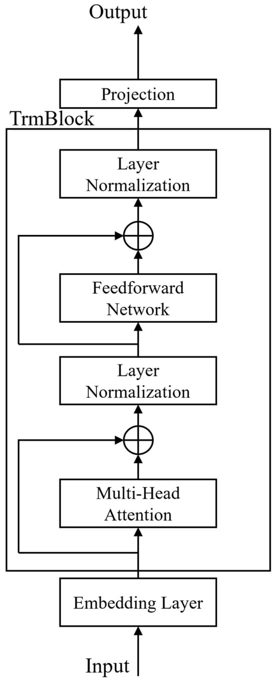
Figure 1.
iTransformer structure. The embedding layer maps the input time series into high-dimensional latent representations. The TrmBlock leverages the attention mechanism to model the relationships among multiple variables, while the feedforward network is employed to further capture temporal dependencies. The projection layer outputs the final predictions. ⊕ denotes element-wised addition, specifically referring to residual connection.
The specific workflow of iTransformer is as follows: given an input
(where N is the number of variables and T is the number of time steps),
denotes all variables at time step t, while
is the complete sequence of the n-th features. Traditional Transformer models perform feature embedding on each time step
, whereas iTransformer embeds each variable
instead. Equation (1) represents the embedding layer of iTransformer, which projects the input time series data into a high-dimensional latent representation.
In this formula,
denotes the output of the embedding layer corresponding to the n-th variable, while
represents the collection of embedded representations for the N variables and D denotes the dimension of the feature mapping. This variable-centric embedding strategy emphasizes the interrelationships among variables and is more suitable for multivariate time series forecasting tasks.
Subsequently, the outputs of the embedding layer are input into the multi-head attention mechanism. By analyzing the scores at different positions within the attention matrix, the interrelationships among variables can be revealed. The attention outputs are then passed through a feedforward network to further learn sequence representations and capture dependencies along the temporal dimension. Meanwhile, residual connections and layer normalization are employed to enhance the stability of gradient propagation. The above process corresponds to the TrmBlock shown in Figure 1, which can be stacked multiple times. This procedure is described in Equation (2). Finally, the prediction results are output through the projection layer. The calculation formulas are shown in Equation (3).
where l represents the number of TrmBlock blocks, and
is the output.
2.2. Short-Time Fourier Transform
The Fourier transform is an important mathematical tool with applications in many fields. The main idea of the Fourier transform is to decompose complex time domain signals into the sum of sine waves with different frequencies, amplitudes, and phases. This process reveals the energy distribution and periodic characteristics of the signal in the frequency domain.
Although the Fourier transform performs well in analyzing stationary signals, it has obvious limitations when applied to non-stationary time series. This approach is based on the assumption that the signal’s frequency components remain unchanged over the entire time span, so the obtained spectrum only reflects the global frequency characteristics. When applied to non-stationary data such as financial time series or voice signals, this assumption will lead to the neglect of local changes and short-term fluctuations, making it difficult to accurately capture the dynamic changes in the signal.
To address these limitations, researchers introduced the short-time Fourier transform. By introducing the time window function, the original signal is divided into multiple parts, and the Fourier transform is applied to each part separately. This approach can analyze the local characteristics of the signal. The mathematical expression of STFT is
where
represents the original signal, f is the frequency variable, and
is a window function centered on time t.
In practical application, the type and length of the window function have a key impact on the analysis results. A narrower window provides higher temporal resolution but lower frequency resolution, while a wider window improves frequency resolution at the expense of temporal localization accuracy. Therefore, the selection of window size involves a trade-off between time and frequency resolution.
2.3. Temporal Convolutional Network
A Temporal Convolution Network is a convolution-based model designed for predicting time series data, which is an important extension of CNNs in this field. Compared with RNNs and LSTM, TCNs can significantly mitigate issues such as vanishing and exploding gradients, while offering greater parallel computation capability and training stability. As a result, they demonstrate high efficiency and accuracy in modeling long sequences [25,26]. Structurally, a TCN mainly consists of the following three parts.
- Causal convolution
In time series forecasting tasks, future information should not be used in computations at the current time step, as this would lead to information leakage. However, when using conventional one-dimensional convolutions on time series, the convolution operation may introduce the future information. A TCN uses causal convolution to address this issue. In a causal convolution, the current output is determined only by the current and past inputs, ensuring that no information from future time steps is used. This one-way modeling mechanism is different from the traditional CNN because it strictly follows the temporal order; only the input of the past can affect the present, thus establishing a model with strict temporal constraints. Specifically, for a convolution kernel of size K, the computation of the causal convolution is given by
where
represents the output of causal convolution at time t,
is the weight of the convolution kernel, and
is the input at time t − k.
- 2.
- Dilated convolution
Causal convolution makes the convolution operation constrained in the time dimension. However, the kernel size still limits the model’s modeling length, which is also one of the limitations of CNNs. A standard CNN usually uses the pooling layer to expand the receptive field, but pooling inevitably leads to information loss. In order to solve this problem, TCN introduces dilated convolution, which inserts a gap into the convolution kernels, thus significantly expanding the receptive field. This allows the model to efficiently model temporal dependencies while avoiding increasing the depth of the network. The calculation formula of dilated convolution is as follows:
where
is the output at time t, d denotes the dilation factor,
is the convolution kernel’s weight, and
represents the input at time t − d. The dilated factor determines the degree to which the convolution kernel expands along the time dimension. It usually grows exponentially in different layers of the network, so that the receptive field expands rapidly in deeper layers.
- 3.
- Residual connection block
Increasing network depth can lead to the vanishing gradient problem. In TCN, residual connections are used to mitigate this issue. Specifically, the residual connection adds the input signal to the convolutional layer’s output to ensure that the gradient can be effectively propagated. The calculation formula of the residual connection is as follows:
Here, F(x) denotes the output of the convolution and other processing layers, x is the input sequence, and Activation represents a nonlinear activation function, which is typically implemented as ReLU in this study. Figure 2 illustrates the architecture of the residual block, each block containing two dilated causal convolution layers, a weight normalization layer, an activation function layer, and a dropout layer. A typical TCN model consists of several residual connection blocks stacked in sequence. Finally, map the high-dimensional features to the required dimensions through the full connection layer and output the results.
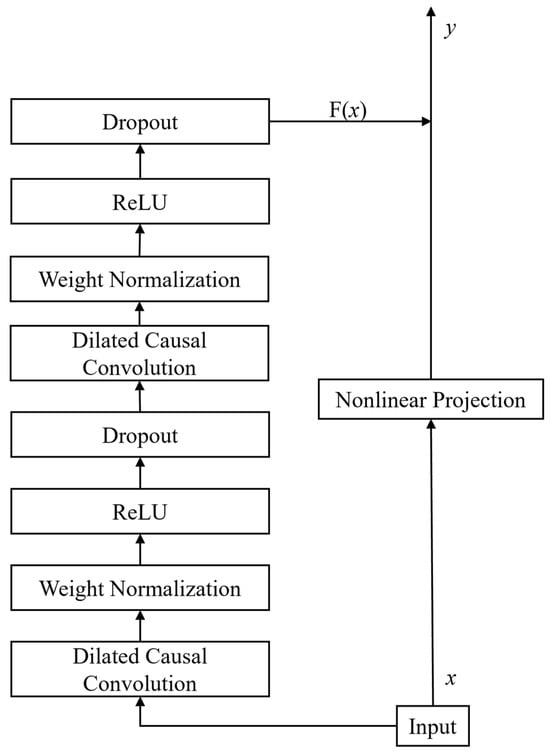
Figure 2.
Residual connection block structure.
2.4. Proposed Model
In this research, we innovatively propose FT-iTransformer. This model is based on time–frequency domain collaborative analysis to achieve accurate prediction of stock prices. FT-iTransformer is designed to comprehensively extract multi-scale features from stock data and to effectively capture the complex relationships among multiple variables, thereby achieving high-accuracy forecasting of future closing prices. FT-iTransformer consists of three main modules: a frequency domain feature extraction module, a multi-scale temporal convolution module, and an iTransformer module. Figure 3 shows the overall structure of FT-iTransformer.
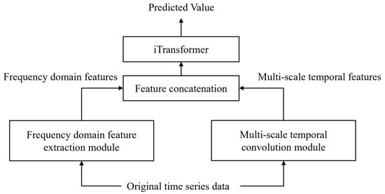
Figure 3.
FT-iTransformer structure.
- Frequency domain feature extraction module
Time series data contain not only rich temporal features but also frequency domain information composed of multiple periodic and frequency components. To fully extract the frequency domain characteristics embedded in stock time series, this study introduces a frequency domain feature extraction module into the model. This module first applies STFT to multichannel stock price sequences to obtain time–frequency spectrograms.
After that, the module employs a 1D-CNN to process the frequency domain information. The convolution operations are performed along the temporal axis to capture the correlations among different frequency components while compressing the high-dimensional spectrogram into more representative feature representations. Subsequently, pooling is applied along the temporal dimension to aggregate the extracted features and ensure temporal alignment between the frequency domain output and the original input. This process not only preserves the essential frequency domain information embedded in multichannel stock data but also provides a strong basis for subsequent joint modeling of time–frequency domain features. Figure 4 shows the structure of the frequency domain feature extraction module.
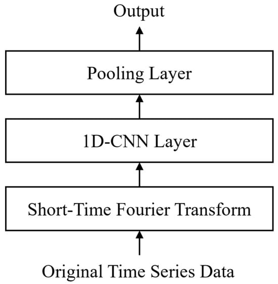
Figure 4.
Frequency domain feature extraction module structure.
- 2.
- Multi-scale temporal convolution module
Stock price time series typically include temporal patterns at multiple scales. To comprehensively extract temporal information across different scales, this study designs an MSTCN module to capture hierarchical time domain features from the original sequence. The module consists of three parallel TCN branches. The size of the convolutional kernel is 3, 5, and 7, respectively, corresponding to different temporal receptive fields: the smaller convolutional kernel captures short-term price fluctuations, while the larger convolutional kernel captures long-term trend changes. Through this multi-scale parallel structure, the model can learn temporal representations of multiple scales simultaneously and comprehensively extract time domain information.
Then, the results of the three branches are weighted and integrated to obtain a comprehensive temporal characteristic representation. This method balances the importance of different temporal scales and reduces the potential bias introduced by dependence on any single scale, thus enhancing the robustness of the model in capturing multi-scale dependencies. The resulting temporal features preserve both localized short-term patterns and the broader long-term trends. The structure of the MSTCN module is shown in Figure 5.
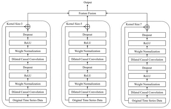
Figure 5.
Multi-scale temporal convolution module structure. ⊕ denotes element-wised addition.
- 3.
- iTransformer module
To fully leverage the extracted time–frequency domain information, this module first concatenates the outputs of the previous two components to form a multi-scale feature tensor, which is then fed into the iTransformer. iTransformer applies an attention mechanism along the feature dimension, allowing each feature to interact with others and thereby capturing the potential relationships among different characteristics of the stock price sequence. Subsequently, the feedforward network further strengthens the capability of the model to learn temporal dependencies, while residual connections and layer normalization ensure stable training. Finally, a projection layer is used to output the predictive value of the closing price.
- 4.
- Design rationale and module collaboration
The importance of each module in FT-iTransformer lies in the complementary information it contributes to the whole prediction task.
The frequency domain feature extraction module enables the model to obtain the frequency characteristics of the input sequence. These features are often difficult to obtain directly from time domain analysis. This enables the model to learn more abundant feature representations, which is very important for modeling nonlinear and non-stationary stock price data.
The MSTCN module focuses on extracting multi-scale temporal features. Compared with the single-scale model, the multi-scale design can simultaneously obtain the short-term fluctuations and long-term trends in the input series, and provide more comprehensive time information. At the same time, this design is also conducive to mitigating the potential deviation introduced by relying on a single time scale.
The above two modules play a complementary role. The frequency domain feature extraction module introduces rich frequency domain information, while the MSTCN module provides the essential temporal representations, which is the basis of time series prediction. Subsequently, iTransformer integrates the outputs of these two components and learn the relationships between different variables and the target variable through the attention mechanism. In addition, iTransformer can further model the temporal dependencies through the feedforward network.
In summary, FT-iTransformer provides a comprehensive modeling framework for stock time series through three core modules. The frequency domain feature extraction module captures latent frequency characteristics within the time series, the MSTCN module is capable of extracting multi-scale time domain information, and iTransformer effectively integrates time–frequency domain features while modeling the complex relationships among multiple variables. Based on this design, FT-iTransformer demonstrates predictive stability when handling highly noisy, volatile, and non-stationary stock price data, offering a feasible solution for stock price prediction.
3. Experiments
3.1. Experimental Environment and Data
In this study, all the experiments were conducted on a Alienware m16 Laptop (Dell (China) Co., Ltd., Xiamen, China) equipped with an Intel Core i9-13900HX CPU (2.20 GHz), an NVIDIA GeForce RTX 4090 GPU (16 GB), and 64GB physical memory. The programming language was Python (v3.9.20), and data visualization adopted Matplotlib (v3.9.2).
This study focuses on six popular stocks in Mainland China and the United States: the SSE Index, LaoFengXiang, Bank of China, SAIC Motor, Apple Inc., and NIKE. The SSE Index, as a representative index reflecting the overall trend of the Shanghai Stock Exchange, is widely regarded as a “barometer” of the performance of the Chinese stock market and attracts significant investor attention. The other five stocks are leading companies in the gold and precious metals, financial, automotive manufacturing, science and technology, and clothing sectors, respectively. These companies occupy important market positions in their industries, and their stock price fluctuations can reflect the characteristics of the industry and investor behavior. In addition, these industries have received wide attention from investors, trading activities are very active, and their price movements can reflect the overall market sentiment and investment decisions. The selected data is from 4 January 2012 to 31 December 2024, including the following features: closing price, opening price, highest price, lowest price, trading volume, and amount. All data we use comes from Tushare. The number of training, validation, and test samples for each dataset is provided in Table 1.

Table 1.
Number of training, validation, and test samples for each dataset.
Figure 6, Figure 7, Figure 8 and Figure 9 illustrate the closing-price trends of some selected datasets. As shown in the figures, the closing price of each dataset has gone through various typical fluctuation stages, including rise, fall, and shock, showing non-stationarity and nonlinear characteristics. This indicates that the selected data is representative and accurately reflects the changing characteristics of the stock market.
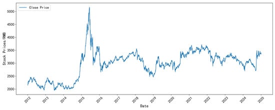
Figure 6.
The closing price of the SSE index dataset.
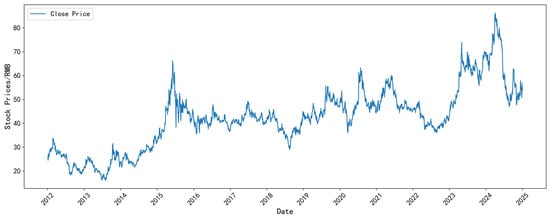
Figure 7.
The closing price of the LaoFengXiang dataset.
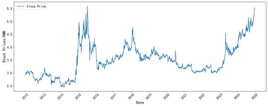
Figure 8.
The closing price of the Bank of China dataset.
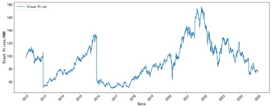
Figure 9.
The closing price of the NIKE dataset.
3.2. Data Preprocessing
In the data preprocessing stage, the original data were cleaned up to remove missing values and duplicate records. Subsequently, each feature was standardized to eliminate the effects of scale differences on the model training. The standardization formula for each variable x is as follows:
where
and
represent the mean and standard deviation of the feature, respectively. Finally, the dataset was partitioned into training, validation, and test subsets using a 7:2:1 ratio.
3.3. Evaluation Metrics
In order to provide a comprehensive evaluation of FT-iTransformer’s performance in predicting stock prices, this study used three evaluation metrics: Mean Absolute Error (MAE), Root Mean Square Error (RMSE), and Mean Absolute Percentage Error (MAPE).
MAE calculates the absolute value of the difference between the predictive value and the actual value. A smaller MAE indicates that the predictive values are closer to the actual values, corresponding to higher predictive accuracy. The mathematical expression is given by
RMSE measures the overall deviation between the predictive value and the actual value. It is particularly sensitive to large prediction errors. Therefore, RMSE can effectively reflect the robustness of the model’s forecasting performance. A smaller RMSE represents better predictive performance. The formula is expressed as follows:
MAPE reflects the average percentage deviation of the predictive value from the actual value. This indicator is easy to explain and helps to compare the model performance on different datasets. A lower MAPE indicates higher predictive accuracy. The formula can be written as
In the above formulas,
is the actual value,
denotes the model’s prediction value, and n represents the number of samples.
3.4. Predictive Performance
To assess the predictive capability of the proposed FT-iTransformer (i.e., ours) in stock price-forecasting, comparative experiments are carried out on six datasets. The experimental results are presented in Table 2, Table 3 and Table 4. The baseline models selected for comparison can be divided into two categories: (1) classic deep learning models, including LSTM, GRU, and TCN. All models in this group were trained for 100 epochs with an early stopping strategy; (2) Transformer-based architectures, including Transformer, Informer, Autoformer, FEDformer, and iTransformer. All models in this group were trained for 30 epochs with an early stopping strategy. The number of parameters of FT-iTransformer is about 54,000. In the experiment, fixed seed points were used for random initialization to ensure the comparability of experimental results.
Table 2.
The predictive results of each model on the SSE Index and LaoFengXiang datasets.
Table 3.
The predictive results of each model on the Bank of China and SAIC Motor datasets.
Table 4.
The predictive results of each model on the Apple Inc. and NIKE datasets.
- LSTM [4]: As a classical variant of RNN, LSTM introduces a gating mechanism, which effectively alleviates the common problems of gradient explosion and vanishing during RNN training. It can capture long-term dependencies and has become the most representative time series prediction model.
- GRU [5]: As another variant of RNN, GRU has a simpler structure and also employs a gating mechanism to mitigate the vanishing and exploding gradient issues. It has been widely used in the field of time series forecasting.
- TCN [6]: As a variant of CNN, TCN employs a convolutional architecture. It uses causal dilated convolution to model temporal dependencies. TCN has the advantages of high parallel computing efficiency and strong modeling stability.
- Transformer [27]: As an encoder–decoder architecture model, Transformer uses the self-attention mechanism to model the temporal dependencies in the time series. This enables the model to better learn the global context relationship.
- Informer [28]: It introduces the ProbSparse self-attention mechanism and attention distilling strategy on the basis of the standard Transformer. These improvements significantly reduce the computational complexity of attention operations, thus improving the efficiency of training.
- Autoformer [29]: It introduces a time series decomposition module in the Transformer framework. Meanwhile, the autocorrelation mechanism is used to replace the self-attention mechanism. Autoformer decomposes the input sequence into trend and seasonal components, and then utilizes autocorrelation to learn the temporal dependencies and periodic patterns.
- FEDformer [30]: It adopts a frequency-enhanced decomposition strategy. The strategy projects the time series data to the frequency domain, enabling the model to capture global trends and high-frequency fluctuations simultaneously. This allows the model to obtain richer feature representations.
- iTransformer [24]: It inverts the role of two important components in the Transformer architecture. iTransformer applies self-attention to model the relationships among various input variables while utilizing a feedforward network to learn temporal dependencies. This framework offers a feasible solution for multivariate time series forecasting.
Overall, FT-iTransformer achieved superior predictive performance and stability across all datasets, outperforming the baseline models across all evaluation metrics. Compared with the best-performing baseline model, iTransformer, FT-iTransformer achieved average reductions of 9.38% in MAE, 9.19% in RMSE, and 9.99% in MAPE. These improvements demonstrate that the integration of the frequency domain feature extraction module and the MSTCN module significantly enhanced the model’s capability in feature representation and temporal dependencies modeling. The results verify that the improvement of iTransformer in this article is effective.
Specifically, among the classical deep learning models, LSTM, GRU, and TCN achieved relatively good results on certain datasets; however, their generalization capability was limited. For example, on the SSE Index and Bank of China datasets, the RMSE values of the LSTM and TCN models increase by 68.27% and 66.79%, and by 74% and 54.92%, respectively, when compared with FT-iTransformer. This phenomenon shows that such models are difficult to adapt to the high dynamics and complexity of financial time series, resulting in considerable fluctuations in prediction errors under different market conditions.
In the model based on the Transformer framework, Transformer and Informer did not perform well on most datasets. Compared with FT-iTransformer, their RMSE values increased by an average of 75.44% and 126.1%, respectively. This indicates that although the standard Transformer framework has strong feature learning capabilities, it is still difficult to model temporal dependencies and complex nonlinear patterns in sequence. Models such as Autoformer, FEDformer, and iTransformer have been optimized (such as sequence decomposition and autocorrelation mechanisms), which have improved stability and prediction accuracy to a certain extent. Compared with this kind of model, the RMSE value of the proposed model decreased by 52.49% on average. These results show that FT-iTransformer always maintains the highest predictive accuracy and stability in all datasets. Even in the case of violent market volatility, FT-iTransformer can capture the fluctuations and trends of stock prices, showing strong stability and generalization ability.
To further verify the statistical significance of model performance improvement, this paper used the Diebold–Mariano (DM) test to compare the prediction results of FT-iTransformer and the optimal baseline model iTransformer on six datasets. The DM test results show that the performance improvement of the proposed model is statistically significant compared with iTransformer on four datasets. Although the differences are not statistically significant on the other two datasets (the SSE Index and Apple Inc.), the DM statistics remain negative, indicating that the overall performance of FT-iTransformer is still better than that of iTransformer. Overall, the DM test provides strong statistical evidence supporting the effectiveness and stability of the proposed model.
To more comprehensively illustrate the predictive capability of the proposed FT-iTransformer, Figure 10 shows the comparison between the actual closing prices and the predictive value of FT-iTransformer on six datasets. In the figure, the blue solid line represents the actual closing prices, and the red dashed line denotes the model’s prediction value. As shown in the figure, the two curves show a highly consistent overall trend, indicating that the model can effectively track the market trend and accurately capture price changes during most time periods. These results demonstrate that FT-iTransformer has stability and superiority under different market conditions, and prove the effectiveness of the model in handling complex financial time series prediction tasks.
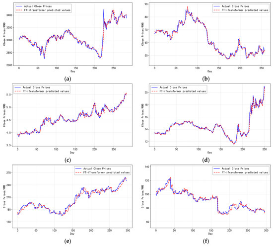
Figure 10.
(a–f), respectively, present the comparison between the actual closing prices and the predictive values generated by the proposed FT-iTransformer model on the SSE Index, LaoFengXiang, Bank of China, SAIC Motor datasets, Apple Inc., and NIKE.
In summary, among all the baseline models, FT-iTransformer consistently achieves the best performance across all datasets. This not only demonstrates the superior predictive capability of the model but also indicates its strong generalization ability under varying market conditions. These results indicate the effectiveness and robustness of the time–frequency domain collaborative modeling.
3.5. Ablation
- Impact of different model components
To evaluate the impact of each module of FT-iTransformer on overall predictive performance, this study conducted a series of ablation experiments. Through the gradual removal or replacement of core modules within the model, the experiments assessed the contribution of each component to the task of stock closing-price prediction.
In terms of experimental setup, the complete FT-iTransformer model was used as the baseline, referred to as Experiment 1, to evaluate the model’s performance when both time–frequency domain features were integrated. In Experiment 2, the frequency domain feature extraction module was removed while retaining the MSTCN module, in order to assess the contribution of frequency domain features to predictive accuracy. Conversely, in Experiment 3, the MSTCN module was removed while keeping the frequency domain feature extraction module, thereby evaluating the importance of the MSTCN module.
Furthermore, to investigate the impact of the multi-scale design on time domain feature modeling, Experiment 4 to 6 replaced the MSTCN module with single-scale TCN models using convolution kernels of sizes 3, 5, and 7, respectively. By comparing these variants with the full model, the advantages of the multi-scale convolutional structure in capturing information across different temporal scales can be assessed. Table 5 presents the specific configurations for the ablation experiments, where ✔ indicates that the corresponding module is enabled.
Table 5.
Specific settings for ablation experiments.
To comprehensively evaluate the effectiveness and contribution of each module across different stock datasets, six ablation experiments were carried out on all datasets, with results presented in Table 6, Table 7 and Table 8. Overall, the results demonstrate that FT-iTransformer maintains high predictive accuracy across all datasets and significantly outperforms the comparison models on all evaluation metrics, confirming the effectiveness of the proposed improvements to the iTransformer model.
Table 6.
The results of ablation experiments on the SSE Index and LaoFengXiang datasets.
Table 7.
The results of ablation experiments on the Bank of China and SAIC Motor datasets.
Table 8.
The results of ablation experiments on the Apple Inc. and NIKE datasets.
Compared with the full FT-iTransformer model, removing the frequency domain feature extraction module (Experiment 2) caused a clear decline in overall performance, with the MAE increasing by approximately 8.02% on average and the RMSE rising by about 9.94%. This finding shows that the frequency domain extraction module plays an important role in capturing periodic trends and high-frequency fluctuations in stock price data. This module can capture potential frequency patterns in the sequence. It provides rich frequency domain information for subsequent modeling.
When the MSTCN module was removed (Experiment 3), the model’s performance decreased significantly. The results in Table 6 demonstrate that the prediction accuracy of the model on each dataset is lower than that of the model using time domain information. This phenomenon indicates that iTransformer lacks explicit multi-scale temporal representations provided by the MSTCN module and has to model temporal dependencies from less informative inputs (the output of the frequency domain feature extraction module). In this case, the temporal dependencies learned by the model are not comprehensive, which leads to a significant decline in prediction performance. These findings confirm the fundamental role of explicit time domain information in time series prediction.
In experiments 4 to 6, single-scale TCN models with kernel sizes of 3, 5, and 7 were used to replace the multi-scale TCN model, leading to a significant decrease in overall performance. Notably, these three single-scale models represented different performance levels on different datasets. This may be due to the differences in the fluctuation characteristics of different data. For datasets with frequent short-term fluctuations, smaller kernels are more effective in capturing local changes, while larger kernels are more suitable for identifying data with longer volatility cycles. Although single-scale TCN achieved good performance on some datasets, its overall prediction accuracy was still significantly lower than that of multi-scale TCN. This finding indicates that multi-scale feature fusion has stronger adaptability and generalization capability in modeling complex stock price data.
In order to illustrate the results of the ablation experiments intuitively, Figure 11, Figure 12 and Figure 13 compare the MAE performance of each experiment on the SSE Index, Bank of China, and Apple Inc. dataset. As shown in these figures, the complete FT-iTransformer achieves the lowest MAE. When the MSTCN module is removed, the performance of the model has declined significantly, which may be due to the lack of explicit temporal information. Meanwhile, removing the frequency domain feature extraction module or replacing the multi-scale structure with a single-scale structure leads to a moderate degradation in performance. Although some information is missing, these models still show acceptable prediction performance.
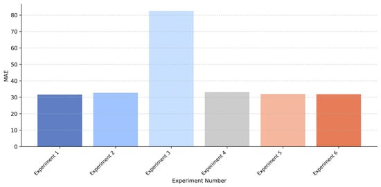
Figure 11.
Comparison of MAE results for each experiment on the SSE Index dataset.
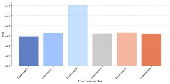
Figure 12.
Comparison of MAE results for each experiment on the Bank of China dataset.
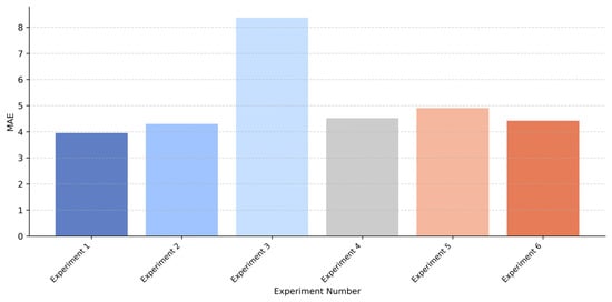
Figure 13.
Comparison of MAE results for each experiment on the Apple Inc. dataset.
- 2.
- Impact of different decomposition methods
In order to further verify the impact of different decomposition methods on the performance of the proposed model, this paper compared STFT with Discrete Wavelet Transform (DWT) on the premise of maintaining the consistency of other experimental settings. Specifically, STFT in the frequency domain feature extraction module was replaced by DWT, and evaluated the model’s prediction performance on all datasets. The experimental results are shown in Table 9.
Table 9.
The ablation results of the decomposition method.
As shown in Table 9, the model employing STFT outperforms its DWT-based counterpart on five datasets. One possible explanation is that STFT is suitable for capturing short-term fluctuations and periodic patterns commonly observed in financial time series. Meanwhile, the performance of DWT depends on the selection of wavelet basis and decomposition level, which may limit its stability across different datasets. The results indicate the effectiveness of using STFT as a decomposition method.
The ablation experiments indicate that the combination of frequency domain features and multi-scale temporal features plays an important role in enhancing model performance. It verifies the rationality and effectiveness of the FT-iTransformer architecture.
3.6. Computational Cost Analysis
To evaluate the computational cost of the FT-iTransformer, this study further compared the average training time of Transformer-based models on all datasets under the same hardware configuration. The experimental results are shown in Table 10.
Table 10.
Average training time of Transformer-based models on all datasets (in seconds).
Table 10.
Average training time of Transformer-based models on all datasets (in seconds).
| Model | Training Time |
|---|---|
| Transformer | 40.5079 |
| Informer | 53.4943 |
| Autoformer | 73.7404 |
| FEDformer | 175.3373 |
| iTransformer | 23.9942 |
| Ours | 93.9676 |
The results indicate that the proposed model requires approximately 93 s for training on average. Compared with Transformer-based models such as Transformer, Informer, and Autoformer, FT-iTransformer is about 1.3 to 2.3 times slower, and it is approximately four times slower than iTransformer, which is the fastest among Transformer-based models. The increase in computational cost is mainly due to the additional frequency domain feature extraction and MSTCN modules, which enhance the model’s ability to capture temporal and frequency domain information. It is worth noting that FT-iTransformer has a faster training speed than FEDformer, which also uses a frequency domain feature extraction method.
In summary, although FT-iTransformer has a moderate increase in training time compared with most Transformer-based models, the significant improvement in prediction accuracy proves the rationality of the increase in computational cost.
3.7. Parameter Sensitivity Analysis
To investigate the sensitivity of FT-iTransformer to key hyperparameters, this section tested the STFT window size (8, 16, 24, 32) and the kernel size (three, four, five, six) of one-dimensional convolution in the frequency domain feature extraction module on three datasets (the SSE Index, LaoFengXiang, and NIKE). Figure 12 illustrates the impact of these hyperparameters on the MAPE values of FT-iTransformer.
As shown in the subfigures (a–c) of Figure 14, FT-iTransformer achieves the best performance on two out of the three datasets when the STFT window size is set to 16, and delivers the second-best performance on the remaining one. Smaller windows may fail to capture long term trends, while larger windows may smooth out short-term fluctuations, both leading to slightly decreased prediction accuracy. From subfigures (d–f) in Figure 12, it can be observed that when the kernel size is three, FT-iTransformer has relatively better results, although larger kernels also provide acceptable performance on some datasets. This indicates that smaller kernels are sufficient to learn the key frequency information.
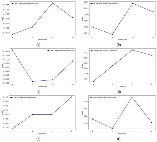
Figure 14.
Sensitivity of FT-iTransformer to STFT window size and convolution kernel size. (a–c) MAPE under different STFT window sizes on the SSE Composite Index, Lao Feng Xiang, and NKE datasets; (d–f) MAPE under different convolution kernel sizes on the same datasets.
In summary, the results show that FT-iTransformer is moderately sensitive to the size of the STFT window and convolution kernel in the frequency domain feature extraction module. Although the performance of FT-iTransformer will fluctuate with the change in hyperparameters, the variations are not very obvious. This demonstrates that FT-iTransformer maintains stable performance across a reasonable range of settings.
4. Conclusions
In this study, we propose a stock price-forecasting model, FT-iTransformer, based on time–frequency domain collaborative analysis. Compared with the existing models, which mainly rely on the time domain information, the proposed model combines the frequency domain features and multi-scale temporal features, so that the model can obtain more abundant information from the input sequence. Meanwhile, FT-iTransformer models the relationship between multiple variables and captures temporal dependencies through iTransformer.
The experimental results on multiple datasets demonstrate that FT-iTransformer consistently outperforms several mainstream time series forecasting models. This indicates that the proposed model can maintain generalization capabilities in different market conditions. The ablation studies further show that explicit multi-scale temporal features play a critical role in improving prediction accuracy. In particular, removing the MSTCN module leads to a clear performance decline, showing that learning temporal dependencies from limited input representations is insufficient for complex financial time series. These findings indicate that time–frequency domain collaborative analysis is an effective strategy for stock price prediction and provides a feasible solution for time series forecasting.
In addition, the proposed model can provide data-driven reference for stock market analysis and auxiliary decision-making for investors, laying a foundation for the application of time–frequency domain collaborative analysis in financial prediction scenarios.
Despite the promising results, this study still has some limitations. Firstly, due to the introduction of the frequency domain information extraction module and the MSTCN module, the computational cost of FT-iTransformer is more than that of some Transformer-based models. Therefore, improving computational efficiency will be an important direction for future work. In addition, the current study mainly focuses on price-related features. Introducing richer features, such as macroeconomic variables or textual data, may further improve the predictive performance of the model.
Finally, we emphasize that no forecasting model can completely overcome the inherent uncertainty of financial markets. Therefore, the model should be regarded as an auxiliary analysis tool, not to replace human judgment in decision-making.
Author Contributions
Conceptualization, Z.Z.; methodology, X.-X.Z.; formal analysis, S.-J.L.; writing—original draft preparation, X.-X.Z.; writing—review and editing, S.-J.L. and C.-Y.H.; supervision, Z.Z.; funding acquisition, S.-J.L. All authors have read and agreed to the published version of the manuscript.
Funding
This research was funded by the Department of Science and Technology of Hunan Province, grant number 2024JJ7549, Xiangxi Vocational and Technical College for Nationalities, grant number 2024KTZ201, Department of Education of Hunan Province, grant number 24C1236, and Department of Science and Technology of Fujian Province, grant number 2025J01670.
Institutional Review Board Statement
Not applicable.
Informed Consent Statement
Not applicable.
Data Availability Statement
The original contributions presented in the study are included in the article; further inquiries can be directed to the corresponding author.
Conflicts of Interest
The authors declare no conflicts of interest.
Abbreviations
The following abbreviations are used in this manuscript:
| Abbreviation | Full Term |
| RNN | Recurrent Neural Network |
| LSTM | Long Short-Term Memory |
| GRU | Gated Recurrent Unit |
| 1D-CNN | One-Dimensional Convolutional Neural Network |
| CNN | Convolutional Neural Network |
| TCN | Temporal Convolution Network |
| MSTCN | Multi-Scale Temporal Convolution Network |
| STFT | Short-Time Fourier Transform |
References
- Neuhann, D.; Sockin, M. Financial Market Concentration and Misallocation. J. Financ. Econ. 2024, 159, 103875. [Google Scholar] [CrossRef]
- Hu, Z.; Zhao, Y.; Khushi, M. A Survey of Forex and Stock Price Prediction Using Deep Learning. Appl. Syst. Innov. 2021, 4, 9. [Google Scholar] [CrossRef]
- Chen, X.; Hu, W.; Xue, L. Stock Price Prediction Using Candlestick Patterns and Sparrow Search Algorithm. Electronics 2024, 13, 771. [Google Scholar] [CrossRef]
- Hochreiter, S.; Schmidhuber, J. Long Short-term Memory. Neural. Comput. 1997, 9, 1735–1780. [Google Scholar] [CrossRef] [PubMed]
- Chung, J.; Gulcehre, C.; Cho, K.; Bengio, Y. Empirical Evaluation of Gated Recurrent Neural Networks on Sequence Modeling. arXiv 2014, arXiv:1412.3555. [Google Scholar] [CrossRef]
- Lea, C.; Flynn, M.D.; Vidal, R.; Reiter, A.; Hager, G.D. Temporal Convolutional Networks for Action Segmentation and Detection. In Proceedings of the 2017 IEEE Conference on Computer Vision and Pattern Recognition (CVPR), Honolulu, HI, USA, 21–26 July 2017; IEEE: New York, NY, USA; pp. 1003–1012. [Google Scholar]
- Gülmez, B. Stock Price Prediction with Optimized Deep LSTM Network with Artificial Rabbits Optimization Algorithm. Expert Syst. Appl. 2023, 227, 120346. [Google Scholar] [CrossRef]
- Md, A.Q.; Kapoor, S.; Chris Junni, A.V.; Sivaraman, A.K.; Tee, K.F.; Sabireen, H.; Janakiraman, N. Novel Optimization Approach for Stock Price Forecasting Using Multi-Layered Sequential LSTM. Appl. Soft Comput. 2023, 134, 109830. [Google Scholar] [CrossRef]
- Farhadi, A.; Zamanifar, A.; Alipour, A.; Taheri, A.; Asadolahi, M. A Hybrid LSTM-GRU Model for Stock Price Prediction. IEEE Access 2025, 13, 117594–117618. [Google Scholar] [CrossRef]
- Chauhan, A.; Shivaprakash, S.J.; Sabireen, H.; Md, A.Q.; Venkataraman, N. Stock Price Forecasting Using PSO Hypertuned Neural Nets and Ensembling. Appl. Soft Comput. 2023, 147, 110835. [Google Scholar] [CrossRef]
- Kanwal, A.; Lau, M.F.; Ng, S.P.H.; Sim, K.Y.; Chandrasekaran, S. BiCuDNNLSTM-1dCNN—A Hybrid Deep Learning-Based Predictive Model for Stock Price Prediction. Expert Syst. Appl. 2022, 202, 117123. [Google Scholar] [CrossRef]
- Biswas, A.K.; Bhuiyan, M.S.A.; Mir, M.N.H.; Rahman, A.; Mridha, M.F.; Islam, M.R.; Watanobe, Y. A Dual Output Temporal Convolutional Network with Attention Architecture for Stock Price Prediction and Risk Assessment. IEEE Access 2025, 13, 53621–53639. [Google Scholar] [CrossRef]
- Zhou, L.; Zhang, Y.; Yu, J.; Wang, G.; Liu, Z.; Yongchareon, S.; Wang, N. LLM-Augmented Linear Transformer–CNN for Enhanced Stock Price Prediction. Mathematics 2025, 13, 487. [Google Scholar] [CrossRef]
- Wang, S. A Stock Price Prediction Method Based on BiLSTM and Improved Transformer. IEEE Access 2023, 11, 104211–104223. [Google Scholar] [CrossRef]
- Haryono, A.T.; Sarno, R.; Sungkono, K.R. Transformer-Gated Recurrent Unit Method for Predicting Stock Price Based on News Sentiments and Technical Indicators. IEEE Access 2023, 11, 77132–77146. [Google Scholar] [CrossRef]
- Zhu, Y. Stock Prediction Method Based on Multi-Source Data of Social Media and Informer Model. In Proceedings of the 2025 International Conference on Digital Management and Information Technology, Shenyang, China, 14–16 March 2025; ACM: New York, NY, USA; pp. 372–377. [Google Scholar]
- Lu, Y.; Zhang, H.; Guo, Q. Stock and Market Index Prediction Using Informer Network. arXiv 2023, arXiv:2305.14382. [Google Scholar] [CrossRef]
- Sheng, Z.; Liu, Q.; Hu, Y.; Liu, H. A Multi-Feature Stock Index Forecasting Approach Based on LASSO Feature Selection and Non-Stationary Autoformer. Electronics 2025, 14, 2059. [Google Scholar] [CrossRef]
- Li, S.; Tang, G.; Chen, X.; Lin, T. Stock Index Forecasting Using a Novel Integrated Model Based on CEEMDAN and TCN-GRU-CBAM. IEEE Access 2024, 12, 122524–122543. [Google Scholar] [CrossRef]
- Qi, C.; Ren, J.; Su, J. GRU Neural Network Based on CEEMDAN–Wavelet for Stock Price Prediction. Appl. Sci. 2023, 13, 7104. [Google Scholar] [CrossRef]
- Tao, Z.; Wu, W.; Wang, J. Series Decomposition Transformer with Period-Correlation for Stock Market Index Prediction. Expert Syst. Appl. 2024, 237, 121424. [Google Scholar] [CrossRef]
- Zhao, Q.; Li, H.; Liu, X.; Wang, Y. A Hybrid Model of Multi-Head Attention Enhanced BiLSTM, ARIMA, and XGBoost for Stock Price Forecasting Based on Wavelet Denoising. Mathematics 2025, 13, 2622. [Google Scholar] [CrossRef]
- Zeng, A.; Chen, M.; Zhang, L.; Xu, Q. Are Transformers Effective for Time Series Forecasting? In Proceedings of the AAAI Conference on Artificial Intelligence, Washington, DC, USA, 7–14 February 2023. [Google Scholar]
- Liu, Y.; Hu, T.; Zhang, H.; Wu, H.; Wang, S.; Ma, L.; Long, M. iTransformer: Inverted Transformers Are Effective for Time Series Forecasting. arXiv 2024, arXiv:2310.06625. [Google Scholar] [CrossRef]
- Hewage, P.; Behera, A.; Trovati, M.; Pereira, E.; Ghahremani, M.; Palmieri, F.; Liu, Y. Temporal Convolutional Neural (TCN) Network for an Effective Weather Forecasting Using Time-Series Data from the Local Weather Station. Soft Comput. 2020, 24, 16453–16482. [Google Scholar] [CrossRef]
- Ao, X.; Gong, Y.; He, A. A Review of Time Series Prediction Models Based on Deep Learning. IEEE Access 2025, 13, 153696–153712. [Google Scholar] [CrossRef]
- Vaswani, A.; Shazeer, N.; Parmar, N.; Uszkoreit, J.; Jones, L.; Gomez, A.N.; Kaiser, Ł.; Polosukhin, I. Attention Is All You Need. In Proceedings of the Advances in Neural Information Processing Systems (NIPS), Long Beach, CA, USA, 4–9 December 2017. [Google Scholar]
- Zhou, H.; Zhang, S.; Peng, J.; Zhang, S.; Li, J.; Xiong, H.; Zhang, W. Informer: Beyond Efficient Transformer for Long Sequence Time-Series Forecasting. In Proceedings of the AAAI Conference on Artificial Intelligence, Virtual, 2–9 February 2021. [Google Scholar]
- Wu, H.; Xu, J.; Wang, J.; Long, M. Autoformer: Decomposition Transformers with Auto-Correlation for Long-Term Series Forecasting. In Proceedings of the Advances in Neural Information Processing Systems (NIPS), Virtual, 6–14 December 2021. [Google Scholar]
- Zhou, T.; Ma, Z.; Wen, Q.; Wang, X.; Sun, L.; Jin, R. FEDformer: Frequency Enhanced Decomposed Transformer for Long-Term Series Forecasting. In Proceedings of the International Conference on Machine Learning (ICML), Baltimore, MD, USA, 17–23 July 2022. [Google Scholar]
Disclaimer/Publisher’s Note: The statements, opinions and data contained in all publications are solely those of the individual author(s) and contributor(s) and not of MDPI and/or the editor(s). MDPI and/or the editor(s) disclaim responsibility for any injury to people or property resulting from any ideas, methods, instructions or products referred to in the content. |
© 2026 by the authors. Licensee MDPI, Basel, Switzerland. This article is an open access article distributed under the terms and conditions of the Creative Commons Attribution (CC BY) license.