Physiological Artifact Suppression in EEG Signals Using an Efficient Multi-Scale Depth-Wise Separable Convolution and Variational Attention Deep Learning Model for Improved Neurological Health Signal Quality

Abstract

Artifacts remain a major challenge in electroencephalogram (EEG) recordings, often degrading the accuracy of clinical diagnosis, brain computer interface (BCI) systems, and cognitive research. Although recent deep learning approaches have advanced EEG denoising, most still struggle to model long-range dependencies, maintain computational efficiency, and generalize to unseen artifact types. To address these challenges, this study proposes MDSC-VA, an efficient denoising framework that integrates multi-scale (M) depth-wise separable convolution (DSConv), variational autoencoder-based (VAE) latent encoding, and a multi-head self-attention mechanism. This unified architecture effectively balances denoising accuracy and model complexity while enhancing generalization to unseen artifact types. Comprehensive evaluations on three open-source EEG datasets, including EEGdenoiseNet, a Motion Artifact Contaminated Multichannel EEG dataset, and the PhysioNet EEG Motor Movement/Imagery dataset, demonstrate that MDSC-VA consistently outperforms state-of-the-art methods, achieving a higher signal-to-noise ratio (SNR), lower relative root mean square error (RRMSE), and stronger correlation coefficient (CC) values. Moreover, the model preserved over 99% of the dominant neural frequency band power, validating its ability to retain physiologically relevant rhythms. These results highlight the potential of MDSC-VA for reliable clinical EEG interpretation, real-time BCI systems, and advancement towards sustainable healthcare technologies in line with SDG-3 (Good Health and Well-Being).

1. Introduction

Electroencephalography (EEG) is an essential tool in neuroscience and clinical practice that provides high temporal resolution insights into brain dynamics and cognitive functions. However, EEG signals are frequently contaminated by several physiological and motion-related artifacts that distort the underlying neural activity and compromise the reliability of the subsequent analyses. Ocular artifacts, such as eye blinks and movements, dominate low-frequency components, whereas muscle artifacts from jaw clenching, neck movements, or other muscle contractions can introduce high-frequency interference across multiple channels. Cardiac artifacts caused by heart activity appear as regular, rhythmic disturbances in EEG signals. Motion-related and other external disturbances can cause sudden signal changes or baseline shifts, severely affecting the clinical and brain computer interface (BCI) performance. In addition, such distortions can critically compromise downstream analyses, particularly in single-channel and wearable EEG systems where manual inspection and multichannel corrections are impractical. Effective artifact suppression is thus crucial for improving EEG interpretability and diagnostic reliability.

Artifact removal from EEG signals has been extensively studied using both signal processing- and deep learning (DL)-based approaches. Traditional artifact removal methods, such as regression [1], adaptive filtering [2], independent component analysis (ICA) [3], canonical correlation analysis (CCA) [4], wavelet transforms [5], and empirical mode decomposition (EMD) [6,7], have been widely employed in EEG processing toolkits (for instance, EEGLAB, FieldTrip, Brainstorm). Although these approaches have proven effective in controlled settings, they often rely on strong assumptions (for instance, source independence in ICA [8]), require manual intervention, and are less effective for single-channel recordings. Hybrid methods combining wavelet transform, EMD, ensemble EMD, variational mode decomposition (VMD), and statistical techniques (ICA and CCA) improve accuracy but remain limited by high computational cost and lack of adaptability to multiple artifact types [9,10,11,12,13].

Recent advances in deep learning have led to data-driven EEG artifact removal methods that automatically learn spatiotemporal relationships from raw signals. Conventional neural networks (CNNs) were among the earliest architectures used in this task. CNN-based models such as 1D-ResCNN [14], Novel-CNN [15], and MMNNet [16] have improved feature extraction and achieved a strong baseline performance. However, they remained limited in modeling long-term temporal dependencies and generalized poorly to unseen noise conditions. Subsequent variants, including optimization-driven models such as ‘Spider Monkey-based Electric Fish optimization’ [17] and DTPNet [18], attempted to enhance feature selection and denoising precision; however, they required extensive training time and large datasets.

Autoencoder-based models include sparse autoencoders [19], stacked sparse autoencoders [20], gated recurrent unit (GRU)-based autoencoders [21], and deep denoising autoencoders [22], all of which demonstrate the ability to preserve background neural activity while removing ocular and muscle artifacts, yet are deterministic and prone to overfitting. Generative adversarial networks (GANs) have further advanced artifact removal through adversarial learning [23], as demonstrated by EEGANet [24], AR-WGAN [25], and FLANet [26]. These models successfully removed ocular, cardiac, and muscular artifacts without additional reference channels; however, they remain difficult to train, are sensitive to hyperparameters, and data-intensive. Several hybrid architectures have emerged to capture both local and global dependencies in EEG [27,28,29,30,31,32]. However, these models typically involve significant computational requirements.

More recently, transformer-based architectures such as EEGDNet [33] and Denosieformer [34] introduced a self-attention mechanism to effectively model long-range temporal dependencies. While these models attained state-of-the-art performance in single-channel denoising, their high computational cost and dependency on large, paired datasets limit their deployment in real-time or embedded systems.

1.1. Motivation and Research Gap

Despite significant advances, existing deep learning-based EEG denoising methods face three critical challenges:

• Limited modeling of long-range temporal dependencies—CNN-based methods primarily capture local patterns, missing sustained drift and burst characteristics.
• Poor generalization to unseen or mixed artifacts—many models overfit training distributions and perform poorly on real-world motion artifacts.
• The trade-off between accuracy and efficiency—transformer models capture the global structure but are computationally heavy and unsuitable for real-time or embedded EEG systems.

1.2. Proposed Solution and Contribution

To address these challenges, the proposed model integrates the following:

• Multi-scale depth-wise separable convolution (DSConv) for compact and efficient spectral–temporal feature extraction.
• Variational autoencoder-based latent space for robust probabilistic representation learning and improved generalization across subjects and datasets.
• A multi-head self-attention mechanism is used to model long-range temporal dependencies and adaptively suppress nonstationary artifacts without distorting the neural components.

This unified architecture effectively balances denoising accuracy, computational efficiency, and generalization capability, thereby addressing the longstanding trade-off in EEG artifact suppression.

The significant contributions of this work are summarized as follows:

• A unified deep learning model for effective EEG denoising.
• The model effectively suppresses physiological artifacts and achieves superior quantitative performance across diverse datasets, including EEGdenoiseNet, Motion Artifact Contaminated Multichannel EEG, and PhysioNet Motor Movement/Imagery datasets, consistently improving the SNR, reducing the RRMSE, and enhancing the CC relative to the current state-of-the-art denoising methods under both synthetic and real-world conditions.
• The model attained >99% preservation of physiologically relevant frequency bands and demonstrated strong cross-subject and cross-dataset robustness.
• The MDSC-VA model achieved high accuracy with only ~2 million parameters, making it suitable for real-time and portable EEG applications.

Unlike deterministic attention mechanisms in prior transformer-based models, MDSC-VA introduces a ‘Kullback–Leibler’ (KL)-regularized variational bottleneck. This probabilistic design allows uncertainty-aware weighting of temporal dependencies and improves the generalization to unseen artifacts.

The rest of this paper is structured as follows: Section 2 details the proposed model architecture and datasets, Section 3 describes the experimental setup and evaluation strategy, Section 4 presents the experimental results and discussions, and Section 5 concludes the study with implications for future work and clinical deployment.

2. Materials and Methods

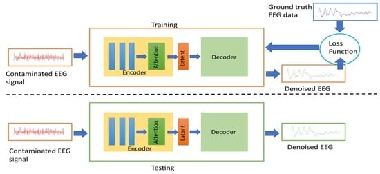
The architecture of the proposed model is shown in Figure 1. Given a contaminated EEG signal $x\in {\mathbb{R}}^{C\times T}$, where C denotes the number of channels and T is the number of time samples, the encoder extracts multi-scale features, applies attention-based contextual weighting, and maps the representation into a latent Gaussian distribution characterized by the mean $\mu \left(x\right)$ and variance ${\sigma }^2\left(x\right)$ as follows:

$$q_{\varphi }\left(z|x\right)=N(z;\mu \left(x\right),{\sigma }^2\left(x\right)I)$$

(1)

where $q_{\varphi }\left(z|x\right)$ represents the approximate posterior distribution produced by the encoder. $z\in {\mathbb{R}}^{d_z}$ is a latent variable that encodes the artifact-free distribution.

Figure 1. The architecture of the proposed denoising model integrating multi-scale DSConv, variational latent representation, and attention module.

While prior models such as EEGDNet and Denosieformer employ deterministic multi-head self-attention, they do not incorporate uncertainty modeling within the attention process itself. The proposed MDSC-VA extends this paradigm by treating the attention outputs as stochastic representations, each of which is modeled as a latent Gaussian variable parameterized by its mean and variance, and regularized via the KL divergence to a unit Gaussian prior. This design embeds uncertainty estimation directly inside the attention mechanism, transforming it into a probabilistic feature selector that adaptively weights temporal dependencies according to their confidence. Consequently, MDSC-VA captures distributional uncertainty, smooths attention responses, and mitigates overfitting to artifact-specific morphologies. The decoder then reconstructs the clean EEG signal $\widehat{y}$ by sampling the latent representation $z$ from the posterior distribution $q_{\varphi }\left(z|x\right)$ as follows:

$$\widehat{y}=p_{\theta }\left(x|z\right)$$

(2)

This probabilistic reconstruction enables the network to generate artifact-suppressed EEG signals that retain the underlying neural information while minimizing overfitting to specific noise patterns. Thus, the denoising process is modeled as

$$\widehat{y}={Decoder}_{\theta }(z~q_{\varphi }\left(z|x\right))$$

(3)

Although several existing studies employ semisynthetic datasets for training [16,33], their models frequently exhibit poor generalizability when applied to unseen real-world EEG recordings. In contrast, the proposed MDSC-VA model was explicitly optimized to overcome this generalization gap. It is trained on semisynthetic contaminated EEG segments, allowing precise control of artifact to signal ratios and rigorously tested on two independent open-source real datasets containing real ocular, muscle, and motion artifacts. This two-phase evaluation demonstrates the capability of the model to adapt to realistic and heterogeneous artifact sources, achieving robust cross-dataset generalization without retraining. Furthermore, by employing depth-wise separable convolutions and variational attention, the network attains state-of-the-art denoising performance with significantly lower computational complexity and memory requirements than traditional CNN- or transformer-based models.

2.1. Multi-Scale Depth-Wise Separable Convolutional Encoder

Artifacts such as ocular activity, myogenic bursts, and motion-induced distortions appear across diverse spectral and temporal scales in EEG recordings. To effectively capture these heterogeneous characteristics, the encoder of the proposed MDSC-VA model integrates a multi-scale feature extraction module (MFE) based on depth-wise separable convolutions (DSConv). For the input EEG segment $x\in {\mathbb{R}}^{C\times T}$, the encoder employs three parallel DSConv branches with kernel sizes $k\in \left\{3,5,7\right\}$, each designed to capture features at a distinct temporal resolution. The operation of each branch can be expressed as follows:

$$h^{\left(k\right)}=f_{DSConv}^{\left(k\right)}\left(x\right),k\in \left\{3,5,7\right\}$$

(4)

where $h^{\left(k\right)}\in {\mathbb{R}}^{C^{\prime }\times T^{\prime }}$ represents the feature map extracted at scale $k$. Each DSConv operation factorizes a standard convolution into depth-wise and pointwise (1 × 1) convolution, thereby reducing the computational cost while preserving discriminative capacity:

$$f_{DSConv}\left(x\right)=f_{pointwise}\left(f_{depthwise}\left(x\right)\right)$$

(5)

where $f_{depthwise}:{\mathbb{R}}^{C\times T}\to {\mathbb{R}}^{C\times T^{\prime }}$ applies a distinct spatial–temporal filter to each channel, learning channel-specific artifact patterns, and $f_{pointwise}:{\mathbb{R}}^{C\times T^{\prime }}\to {\mathbb{R}}^{C^{\prime }\times T^{\prime }}$ performs a $1\times 1$ convolution to combine channel-wise information linearly.

Outputs from all scales are concatenated and normalized to produce the integrated multi-scale representation:

$$h=Concat\left(h^{\left(3\right)},h^{\left(5\right)},h^{\left(7\right)}\right),h\in {\mathbb{R}}^{C_{concat}\times T^{\prime }}$$

(6)

Small kernels ($k$ = 3) captured fine temporal variations and sharp electromyography (EMG) spikes. Medium kernels ($k$ = 5) captured mid-range rhythmic fluctuations, and large kernels ($k$ = 7) captured slow drifts such as ocular artifacts. Each convolution branch was followed by batch normalization and dropout ($p$ = 0.3) to stabilize the optimization and enhance the generalization.

Depth-wise separable convolution reduces the parameter count by approximately 1/$K$ relative to the standard convolution, where $K$ denotes the kernel length (see Appendix A.1 for a detailed formulation). In the MDSC-VA model, three MFE modules are sequentially cascaded to construct a hierarchical encoder. This progressive stacking enriches the feature abstraction from low-level local signals to high-level temporal representations, providing a robust foundation for the subsequent attention-based latent encoding and reconstruction stages. The structural design of the multi-scale feature extraction (MFE) module is illustrated in Figure 2. This encoder design efficiently captured artifact-related patterns across multiple scales while retaining essential EEG features for subsequent contextual modeling.

Figure 2. Structural design of the multi-scale feature extraction (MFE) module.

2.2. Self-Attention Module

While multi-scale feature extraction (MFE) modules effectively capture the localized spectral–temporal characteristics of EEG signals, they are fundamentally limited in modeling long-range dependencies that are crucial for distinguishing spatially distributed artifacts such as eye blinks or motion-induced distortions. To overcome this limitation, the encoder integrates a multi-head self-attention block that adaptively weights temporal segments based on their contextual significance [35].

Given the MFE output $X\in R^{Txd}$, (let $X=h$ from Equation (6)), where $d$ denotes the feature dimension, the attention mechanism derives three learned projections, queries $Q$, keys $K,$ and valus $V,$ through linear transformations: $Q=X{W}^Q$, $K=X{W}^K$, and $V=X{W}^V$ (where $W^Q$, $W^K$, and $W^V\in R^{dx{d}_k}$ are trainable matrices and $d_k$ represents the key dimensionality per head). The scaled dot product is then computed as follows:

$$Attention\left(Q,K,V\right)=Softmax\left({\displaystyle \frac{Q{K}^T}{\sqrt{d_k}}}\right)V$$

(7)

This mechanism enables the proposed model to assign higher attention weights to temporally salient regions, allowing it to focus selectively on informative EEG segments while reducing the influence of redundant components. In practice, this facilitates improved discrimination between artifact- and neural-dominated time intervals. In the proposed model, four attention heads were used (N = 4) and their outputs were concatenated and linearly projected to produce the attended feature representation:

$$h_{attn}=Concat({head}_1,\dots \dots \dots {head}_N)W^o$$

(8)

where $W^o$ $\in R^{N{d}_k\times d}$ denote the trainable output projection. To facilitate stable optimization and residual learning, the attention output is added to its input through a skip connection followed by layer normalization as follows:

$${h^{\prime }=LayerNorm(X+h}_{attn})$$

(9)

This residual normalized formulation enhances gradient propagation and maintains consistency between the original and attention-refined features. The inclusion of a multi-head self-attention block significantly improved the model’s ability to discriminate between artifact-affected and artifact-free temporal regions, leading to a more consistent suppression of different artifacts. Figure 3 illustrates the internal process of the multi-head self-attention mechanism and its interaction with the multi-scale encoder output, resulting in a globally contextualized representation.

Figure 3. The process of the multi-head self-attention mechanism.

2.3. Variational Autoencoder-Based Latent Representation

To enhance generalization and achieve robust separation between neural and artifactual components, the proposed model employs a variational autoencoder-based (VAE) latent representation [36]. In contrast to deterministic encoders, which map inputs into a fixed vector, VAE encodes attention-enhanced EEG features into a probabilistic latent distribution. This enforces a smooth and continuous latent space that captures the statistical regularities of the clean EEG activity. The encoder network parameterized by $\varphi$ maps $h^{\prime }\in R^{T\times d}$ as the output of the self-attention module, to a latent posterior distribution given by the following:

$$q_{\varphi }\left(z|h^{\prime }\right)=N\left(\mu \right(h^{\prime }),{diag(\sigma }^2(h^{\prime }\left)\right))$$

(10)

where $\mu \left(h^{\prime }\right)\in R^L$ and ${\sigma }^2\left(h^{\prime }\right)\in R^L$ represent the mean and standard deviation vectors of the latent distribution, respectively, and L = 64 denotes the latent dimension. To enable differentiable sampling during backpropagation, reparameterization is applied according to the following:

$$z=\mu \left(h^{\prime }\right)+\sigma \left(h^{\prime }\right)\times \epsilon ,\epsilon ~N(0,I)$$

(11)

The decoder $p_{\theta }\left(x|z\right)$, parameterized by $\theta$, reconstructs the denoised EEG signal (as defined in Equation (2)). To ensure a compact and structured latent space, a ‘Kullback–Leibler (KL) divergence’ regularization is imposed between the approximate posterior $q_{\varphi }\left(z|h^{\prime }\right)$ and the unit Gaussian prior $p\left(z\right)=N\left(0,I\right)$ according to Equation (12):

$$L_{KL}=-{\displaystyle \frac{1}{2}}{\sum }_i(1+\log {\sigma }_i^2-{\mu }_i^2-{\sigma }_i^2)$$

(12)

This constraint regularizes the latent distribution towards a unit Gaussian, ensuring smooth transitions in the latent space and minimizing overfitting. Such probabilistic encoding allows the model to represent the uncertainty in EEG features while effectively distinguishing neural activity from nonneural artifact components.

The incorporation of a variational latent representation introduces several advantages over the conventional autoencoder-based denoising approaches. The KL term ensures that both clean and contaminated EEG representations occupy nearby regions in the latent space, thereby facilitating stable reconstruction across varying artifact types. Furthermore, by enforcing a standard Gaussian prior, the model becomes less sensitive to dataset distinction biases, improving generalization across unseen real-world recordings. Figure 4 illustrates the general VAE architecture, utilized to map attention-refined EEG features into a structured latent space and reconstruct clean EEG signals from sampled latent vectors.

Figure 4. The variational autoencoder architecture.

2.4. Loss Functions

The training of the proposed MDSC-VA model was guided by a composite objective function that simultaneously minimized reconstruction error, enforced spectral consistency, and regularized the latent representation. The total loss $L_{total}$ is expressed as follows:

$$L_{total}=L_{MSE}+{\alpha L}_{spec}+\beta L_{KL}$$

(13)

where $L_{MSE}$ denotes the mean square reconstruction loss in the time domain, $L_{spec}$ represents the spectral consistency loss based on short-time Fourier transform (STFT), and $L_{KL}$ corresponds to the KL divergence term (described in Section 2.3). The MSE loss in the time domain is as follows:

$$L_{MSE}={\displaystyle \frac{1}{N}}{\sum }_N{(x-\widehat{y})}^2$$

(14)

This term ensures that the reconstructed EEG $\widehat{y}$ accurately reproduces the temporal morphology of the clean EEG $x$, thereby minimizing the reconstruction error in the signal domain. The spectral consistency loss is defined as follows:

$$L_{spec}={‖\left|S\left(x\right)\right|-\left|S\left(\widehat{y}\right)\right|‖}^2$$

(15)

where $S$(.) denotes the STFT magnitude computed using 50% overlapping Hanning windows. This term preserves the frequency domain information and ensures that physiologically meaningful oscillations are retained after denoising. The weighting parameters were empirically set to $\alpha$= 0.2 and $\beta =0.05$ to balance spectral preservation and latent regularization. This composite formulation ensures that the network learns to suppress artifacts while maintaining the underlying temporal and spectral integrity of the EEG signal.

2.5. Decoder with Skip Connections

The decoder reconstructs the artifact-free EEG signal $\widehat{y}$ from the latent representation $z$ sampled from the posterior distribution $q_{\varphi }\left(z|h^{\prime }\right)$. It performs inverse mapping of the encoding process, progressively upsampling the latent features to recover the temporal resolution of the original EEG signal. Skip connections were incorporated between the corresponding encoder and decoder layers to ensure efficient gradient propagation and retain fine-grained temporal information. These connections directly concatenate or add encoder feature maps to their mirrored decoder counterparts, allowing the decoder to reuse multi-scale contextual information that might otherwise be lost during downsampling.

Mathematically, the reconstruction at each decoder stage $l$ can be expressed as follows:

$$y^{\left(l\right)}=f_{up}^{\left(l\right)}\left(y^{\left(l-1\right)}\right)+g_{skip}^{\left(l\right)}\left(h^{\left(L-l\right)}\right)$$

(16)

where $f_{up}^{\left(l\right)}(.)$ denotes the learnable transposed convolution or upsampling operation at layer $l$, $h^{\left(L-l\right)}$ represents the feature map from the corresponding encoder layer, and $g_{skip}^{\left(l\right)}(.)$ refers to skip connection transformation. This formulation enables the decoder to integrate both global contextual features from deeper latent representations and local structural details from earlier encoder layers, yielding denoised signals that preserve sharp temporal transitions and rhythmic neural features.

In the proposed model, each decoder stage consists of a Conv1DTranspose–BatchNorm–Dropout sequence, followed by additive skip fusion with encoder outputs. The final layer employs 1D convolution with linear activation to generate a continuous EEG reconstruction $\widehat{y}$. Skip connection design stabilizes training by mitigating vanishing gradients and enhances the reconstruction of low-amplitude oscillatory activity, which is often masked by strong artifacts.

The detailed parameters corresponding to each layer of the proposed model are listed in Appendix A.2 (Table A1).

2.6. Data Preparation

To comprehensively train and evaluate the proposed MDSC-VA model, three datasets were utilized as follows: the ‘EEGdenoiseNet dataset’ [37] for training and validation under controlled semisynthetic conditions, the ‘Motion Artifact Contaminated Multi channel EEG dataset’ [38] to test the model performance against real motion-induced artifacts, and the ‘PhysioNet EEG Motor Movement/Imagery (MMI) Dataset’ [39] for large-scale cross-subject generalization. All recordings were synchronized to a uniform sampling rate of 256 Hz and segmented into overlapping 512 sample windows before model processing. A concise overview of all the datasets employed in this study is provided in Table 1.

Table 1. An overview of all datasets employed in this study.

Dataset	Type	Subjects	Channels	Sampling Rate (Hz)	Epoch Length	Artifact Types	Preprocessing Steps	Usage in Study
EEGdenoiseNet [37]	Semisynthetic dataset for supervised denoising	-	Single	512→256	2 s	Ocular (EOG), muscle (EMG), combined (EOG + EMG)	Band pass 1–80 Hz, notch 50/60 Hz, z-score normalization, resample to 256 Hz	Training/validation of EOG, EMG, and combined artifact contamination model
Motion Artifact Contaminated Multi channel EEG dataset [38]	Real artifact dataset with synchronized motion sensors	1 (healthy male)	14 EEG + 9 motion sensors	128	2 s	Eye blink, eyebrow movement, eye movement, head tilt, head shake, leg shake	Band pass 0.5–45 Hz, mastoid reference, resample to 256 Hz, z-score normalization	Testing of trained models under real motion artifacts
PhysioNet EEG Motor Movement/Imagery (MMI) Dataset [39]	Large-scale real EEG for cross-dataset evaluation	109	64 (Biosemi Active Two, 10–20 system)	160→256	2 s	Ocular, muscular, motion	Band pass 0.5–45 Hz, common average reference, z-score normalization	Cross-dataset testing of combined model on all subjects

2.6.1. EEGdenoiseNet Dataset

The ‘EEGdenoiseNet dataset’ [37] provides clean EEG and artifact recordings designed specifically for deep learning-based denoising studies. It consists of 4514 clean EEG segments, 3400 ocular artifact segments, and 5598 muscle artifact segments, each corresponding to a 2 s epoch. The clean EEG signals were obtained from 64 channel motor imagery recordings, originally sampled at 512 Hz, band pass filtered between 1 and 80 Hz, and resampled to 256 Hz. Ocular artifact segments were extracted from electrooculogram (EOG) recordings (filtered 0.3–10 Hz) and muscle artifacts were derived from facial data (filtered 1–120 Hz). Semisynthetic contaminated EEG ($x$) was synthesized using linear superposition as follows:

$$x=\tilde{x}+\lambda \times n$$

(17)

where $\tilde{x}$ denotes the clean EEG, n is the artifact, and $\lambda$ is a scaling factor adjusted to yield the desired signal-to-noise ratio (SNR) according to Equation (18).

$$SNR=10\log {\displaystyle \frac{RMS\left(x\right)}{RMS(\lambda \times n)}}$$

(18)

Contamination was generated within realistic SNR ranges of −7 dB to 2 dB. Three datasets were produced as follows: (1) EEG + EOG (ocular contamination), (2) EEG + EMG (muscular contamination), and (3) EEG + EOG + EMG (combined contamination). Each configuration was divided into 80% training, 10% validation, and 10% testing. This design allowed the model to learn both single-source and mixed-artifact characteristics, enabling strong generalization to unseen artifact types during real-world evaluation.

2.6.2. Motion Artifact Contaminated Multichannel EEG Dataset

To evaluate the robustness of the trained model under real motion artifacts, the ‘Motion Artifact Contaminated Multichannel EEG dataset’ [38] was employed. EEG signals were recorded at the Biomedical Instrumentation and Signal Processing Laboratory, Independent University, Bangladesh, using a 14-Channel Emotive epoch headset (10–20) system equipped with 3 axis accelerometer, gyroscope, and magnetometer sensors. EEG and motion data were simultaneously sampled at 128 Hz across twelve activities introducing different motion artifacts: eye blinking, eyebrow movement, eye movement, talking, listening to music, walking, head shaking, and resting with eyes closed or open.

Each activity file (for instance Sub_EB.mat) contains 14 EEG signals and nine motion channels. The trained MDSC-VA model was evaluated for eye movements and tasks involving muscle activities. This testing ensured that the denoising capability of the model extended to complex real, nonstationary motion artifacts encountered in wearable EEG applications.

2.6.3. PhysioNet EEG Motor Movement/Imagery Dataset

To verify subject independent generalization, the ‘PhysioNet EEG Motor Movement/Imagery dataset’ [39] was used. This dataset contains 64-channel EEG data from 109 healthy participants, recorded using the BCI2000 system, developed by the BCI Research and Development Program at the Wadsworth Center, New York State Department of Health, located in Albany, New York, USA [40]. Each participant performed 14 runs, where R01–R02: baseline, R03–R14: motor movement and motor imagery tasks.

Run 01 was used as the clean reference EEG while runs R03–R014 were treated as contaminated by natural motion and physiological artifacts (ocular, muscular, and body movements). The frontal, central, temporal, and occipital channels (Fp1, Fp2, AF3, AF4, Cz, T7, T8, and Oz) were selected to capture both ocular and myogenic artifact regions. For this study, only the run R03 was selected for testing because it contained pronounced spontaneous ocular and muscular artifacts representative of natural EEG contamination. This section ensures computational efficiency while retaining sufficient variability for statistical analysis, since the dataset includes recordings from 109 distinct participants. Evaluating all subjects within a single artifact-rich run provides a robust measure of cross-subject generalization without the redundancy of multiple runs from the same participant.

3. Experimental Setup

All the experiments were implemented in TensorFlow (v2.19) on a Google Colab GPU environment (NVIDIA Tesla T4, 15 GB). The ADAM optimizer was used with an initial learning rate of 4.5 × 10⁻⁵, momentum parameters β1 = 0.9 and β2 = 0.99, and batch size of 64. Training continued for a maximum of 100 epochs with early stopping (patience = 15 epochs) based on the validation loss. The latent dimension was fixed at 64 (refer to Appendix B), and the attention head count was set to four, ensuring an optimal trade-off between model complexity and representational power.

3.1. Performance Metrics

In this study, four metrics, namely, the signal-to-noise ratio ($SNR$), relative root mean square error ($RRMSE$), correlation coefficient ($CC$), and band power preservation (BP) were utilized for model evaluation.

The $SNR$ evaluates the effectiveness of artifact suppression by comparing the power of the clean EEG signal with that of the residual noise after denoising.

$$SNR\left(\mathrm{d}\mathrm{B}\right)=10\log {\displaystyle \frac{\sum _N{\left(\tilde{x}\right)}^2}{\sum _N{(\tilde{x}-\widehat{y})}^2}}$$

(19)

Higher $SNR$ values indicate better artifact removal and preservation of the neural activity.

The $RRMSE$ quantifies the relative difference between the clean or ground truth EEG $\tilde{x}$ and denoised signal $\widehat{y}$. It normalizes the reconstruction error using the energy of the reference signal, thereby ensuring comparability across subjects and channels.

$$RRMSE={\displaystyle \frac{\sqrt{\sum _N{(\tilde{x}-\widehat{y})}^2}}{\sqrt{\sum _N{\left(\tilde{x}\right)}^2}}}$$

(20)

where $N$ is the sequence length. A lower $RRMSE$ indicates a closer match between denoised and ground truth clean EEG.

The $CC$ measures the linear similarity between the temporal structures of clean EEG and denoised signals.

$$CC={\displaystyle \frac{Cov(\tilde{x},\widehat{y})}{\sqrt{Var\left(\tilde{x}\right)Var\left(\widehat{y}\right)}}}$$

(21)

After denoising, the practical values of $CC$ range from 0 to 1, with values closer to 1 indicating a strong preservation of the signal morphology.

The ability of the proposed model to preserve physiologically relevant rhythms and band power was calculated for the clean EEG and denoised EEG in the dominant frequency bands affected by artifacts. Power spectral density (PSD) was estimated using Welch’s method, and the percentage preservation was computed as follows:

$$Preservation\left(\%\right)=\left(1-{\displaystyle \frac{\left|P_{clean}-P_{denoised}\right|}{P_{clean}}}\right)\times 100$$

(22)

where $P_{clean}$ and $P_{denoised}$ represent the spectral power in the respective frequency bands.

3.2. Statistical Significance Testing

To ensure that the observed improvements achieved by the proposed model were statistically significant, hypothesis-driven evaluations were conducted using parametric and nonparametric tests depending on data normality. The null hypothesis (H₀) assumes that there is no significant difference in denoising performance between the proposed MDSC-VA model and the baseline models across the quantitative metrics ΔSNR, RRMSE, and CC. The alternative hypothesis (H_a) asserts that the proposed MDSC-VA model achieves significantly superior performance compared to all baselines.

Paired t-tests were applied between the pre- and post-denoising metrics for each subject and channel. When normality assumptions were violated (‘Shapiro–Wilk test’, p > 0.05), a ‘Wilcoxon signed rank test’ was used. Additionally, Cohen’s $d$ effect size was computed to quantify the magnitude of the improvement:

$$cohen’sd={\displaystyle \frac{{Metric}_{after}-{Metric}_{before}}{{SD}_{diff}}}$$

(23)

where ${SD}_{diff}$ is the standard deviation of the difference between paired samples. All tests were performed at a significance level of p < 0.05, and results were visualized using ${-\log }_{10}\left(p\right)$ heatmaps and Cohen’s $d$ bar plots for comparative analysis across multiple models.

4. Results and Discussion

4.1. Performance Evaluation

The proposed MDSC-VA model was extensively evaluated and compared with five existing deep learning-based EEG denoising models: 1D Res-CNN [14], Novel-CNN [15], MMNNet [16], EEGDNet [33], and Denosieformer [34]. Each baseline represents a distinct design paradigm, including residual convolutional learning, multi-scale feature extraction, hybrid fully connected modeling, and transformer-based self-attention. To ensure a fair and unbiased comparison, all models were trained, validated, and tested under identical experimental settings, using the same datasets, preprocessing pipelines, training epochs, optimizer configurations, and data partitioning ratios. The models with publicly available code were obtained from the official repositories. The models without available implementations were reproduced based on descriptions in the respective articles. This uniform evaluation protocol enables an equitable assessment of the ability of each mode to achieve artifact suppression, neural signal preservation, and computational efficiency under identical conditions.

4.1.1. Results on EEGdenoiseNet Dataset

The EEGdenoiseNet dataset described in Section 2.6 was used as the principal benchmark to evaluate the proposed model across ocular (EOG), muscular (EMG), and combined (EOG + EMG) artifact conditions under controlled SNR variations. The proposed model and all the baseline models were trained for each contamination type—(1) ocular artifact removal, (2) muscle artifact removal, and (3) combined artifact removal. Figure 5 presents representative examples of denoised EEG waveforms obtained from the proposed MDSC-VA model in comparison with existing deep learning models for the three artifact conditions. In all cases, the proposed model demonstrated the closest morphological resemblance to the ground truth signal.

Figure 5. Sample denoised EEG signal segments under three artifact conditions: (a) EOG (left), (b) EMG (middle), and (c) combined EOG + EMG (right).

While conventional CNN-based approaches, such as 1D Res-CNN and Novel-CNN, suppress large artifact components, they frequently oversmoothen the EEG, attenuating fine oscillatory details. In contrast, the MDSC-VA model effectively removed both low-frequency ocular drifts and high-frequency EMG bursts while maintaining the structural integrity of neural activity, confirming its superior temporal and amplitude reconstruction fidelity. The quantitative results summarized in Table 2 and visualized in Figure 6a–c show the variation in the RRMSE with the input SNR for the three contamination scenarios. Across all SNR levels, the proposed model achieved the lowest RRMSE value of 0.276 for EOG, 0.373 for EMG, and 0.368 for combined artifacts, outperforming all the baselines. This consistent trend across varying noise intensities indicates the strong adaptability of the model to both isolated and composite artifact conditions. Figure 7a–c depict the CC as a function of the SNR for the same cases. The proposed model achieved the highest CC values of 0.962 for ocular artifacts, 0.925 for muscle artifacts, and 0.934 for combined contamination. These improvements confirm that the model not only reduces the error magnitude but also maximizes the similarity with the underlying clean EEG across all noise levels.

Table 2. Average performance metrics for all models on EEGdenoiseNet dataset.

Artifact	Metric	1D Res-CNN	Novel-CNN	MMNNet	EEGDNet	Denosieformer	Proposed Method
EOG	RRMSE	0.446	0.397	0.332	0.391	0.319	0.276
	CC	0.9	0.918	0.942	0.921	0.946	0.962
	ΔSNR (dB)	9.65	11.51	12.42	10.83	12.47	13.49
EMG	RRMSE	0.405	0.401	0.396	0.397	0.393	0.373
	CC	0.902	0.909	0.917	0.913	0.919	0.925
	ΔSNR	8.49	8.71	9.7	8.88	10	10.46
EOG + EMG	RRMSE	0.426	0.419	0.410	0.412	0.377	0.368
	CC	0.906	0.909	0.921	0.917	0.928	0.934
	ΔSNR (dB)	7.42	7.74	7.69	7.55	8.46	8.68

Figure 6. Results on the EEGdenoiseNet dataset at various SNR levels following artifact removal: (a) RRMSE values under ocular artifact removal, (b) RRMSE values under muscle artifact removal, (c) RRMSE values under combined artifact removal.

Figure 7. Results on the EEGdenoiseNet dataset at various SNR levels following artifact removal: (a) CC values under ocular artifact removal; (b) CC values under muscle artifact removal; (c) CC values combined artifact removal.

In addition to time domain reconstruction, the frequency domain integrity was evaluated by assessing the band power preservation ratio in physiologically relevant frequency ranges. As shown in Figure 8a–c, the MDSC-VA model preserved > 99% of the delta, theta, and alpha band power during ocular artifact suppression and >99% of the alpha, beta, and gamma power for muscular and combined artifacts. Such high preservation rates indicate that the model effectively suppressed artifact energy while retaining task-related neural oscillations. In contrast, other CNN- and transformer-based models exhibited noticeable attenuation, particularly in the theta and alpha bands, suggesting a partial loss of neural information. Overall, these results demonstrate that the proposed MDSC-VA framework provides robust denoising performance across diverse artifact conditions, maintaining both the temporal morphology and spectral characteristics of the EEG signals. The combination of multi-scale depth-wise separable convolution and variational attention encoding enables efficient feature extraction and latent regularization, resulting in accurate, generalizable, and physiologically consistent artifact suppression.

Figure 8. Comparison of band power preservation in the dominant frequency band of EEG signals after denoising. (a) Ocular artifact removal, (b) muscle artifact removal, (c) combined artifact removal.

4.1.2. Evaluation of the Motion Artifact Contaminated Multichannel EEG Dataset

To assess the cross-dataset generalization capability of the proposed model, evaluations were performed on a motion artifact contaminated multichannel EEG dataset containing different real-world movement induced artifacts. Six distinct motion activities were analyzed, including eye blink (EB), eyebrow movement (EBM), eye movement (EM), head tilt (HT), head shake (HS), and leg shake (LS), each introducing unique temporal and spectral distortions into the EEG signals. Although denoising was conducted across all 14 EEG channels, Figure 9a,b illustrates representative waveform comparisons for a single channel across these activities. These examples provide qualitative insights into how different networks reconstruct neural signals from motion-corrupted input. Conventional CNN-based models such as 1D Res-CNN and Novel-CNN exhibit either oversmoothing of low-frequency content or residual high-frequency motion components, indicating limited adaptability to dynamics, and nonstationary noise. The MMNNet, EEGDNet, and Denosieformer models show relatively improved artifact suppression but often distort phase alignment or attenuate neural oscillations in the alpha–beta range. In contrast, the proposed MDSC-VA model effectively suppressed transient amplitude bursts and low-frequency drifts while preserving waveform continuity and neural morphology.

Figure 9. (a) Visual representation of denoised single-channel EEG signals across three motion activities (EB, EBM, EM) for different models. (b) Visual representation of denoised single-channel EEG signals across three motion activities (HT, HS, LS) for different models.

Figure 10 presents the box plots of the ΔSNR, RRMSE, and CC for all six activities across the six compared models. In these plots, the central horizontal line represents the median value, the box height indicates the interquartile range (IQR), and the small circles outside the whiskers denote outlier channels showing relatively high artifact coupling (typically frontal or temporal electrodes). Across all motion conditions, the MDSC-VA model exhibited the highest median ΔSNR, lowest RRMSE, and highest CC values while also producing the narrowest IQRs, indicating a more stable performance across EEG channels. For instance, during head tilt and leg shake conditions, where most networks struggled with severe motion contamination, the proposed model maintained smooth neural waveforms with superior reconstruction quality. These observations confirm that the multi-scale feature extraction and variational attention mechanism enable the model to generalize effectively to dynamic and nonstationary motion artifacts, even though it was trained only on synthetic EOG/EMG contamination.

Figure 10. Box plots of (a) ΔSNR, (b) RRMSE, and (c) CC values across six motion conditions for all models.

4.1.3. Evaluation on the PhysioNet EEG Motor Movement/Imagery Dataset

To further examine cross-subject generalization, the proposed MDSC-VA model was evaluated on the PhysioNet EEG Motor movement/Imagery dataset, which includes recordings from 109 participants. Metrics were computed for each channel and averaged across participants to ensure a comprehensive statistical representation. For visualization, Figure 11 presents a representative denoising example from the Fp2 channel of Subject S001, which illustrates the signal reconstruction quality achieved by the proposed model on a real multi-subject dataset. However, the statistical validation summarized in Figure 12a,b was performed across all subjects and channels to capture population-level performance trends. Pairwise comparisons between the proposed and baseline models were conducted for each evaluation metric in accordance with the hypothesis testing framework defined in Section 3.2. Specifically, Figure 12a illustrates the ${-\log }_{10}\left(p\right)$ significance heatmap and Figure 12b shows the Cohen’s $d$ effect size plot. Values of d > 1.5 and ${-\log }_{10}\left(p\right)$ > 2 (p < 0.01) indicate large, statistically significant improvements. The proposed MDSC-VA model consistently yielded strong positive effect sizes across almost all electrodes, particularly in the frontal and temporal regions, the areas most prone to ocular and muscular contamination. These findings lead to the rejection of the null hypothesis and the acceptance of Ha, confirming the statistical superiority and cross-subject robustness of the proposed model.

Figure 11. Single-channel (Fp2, subject S001) denoised waveform example for qualitative illustration.

Figure 12. (a) ${-\log }_{10}\left(p\right)$ statistical significance heatmap, (b) Cohen’s $d$ effect size plot across all channels and subjects.

4.2. Ablation Study

The proposed MDSC-VA architecture integrates three key components—multi-scale feature extraction, latent representation learning, and temporal self-attention, where each component contributes uniquely to artifact suppression and neural preservation. To assess their individual impact, a series of ablation experiments were conducted separately for both ocular and muscle artifact conditions. The following model variants were tested.

• Proposed model: The complete model where the latent dimension is set to 64, with four heads in the self-attention mechanism and all modules included.
• w/o depth-wise separable convolution: This replaces the depth-wise separable convolution with standard convolution layers within the multi-scale feature extraction block.
• w/o multi-scale feature extraction (MFE) block: Proposed model with a single-stage feature extraction block.
• w/o latent representation: It maintains the standard encoder–decoder structure without latent representation z.
• w/o attention module: This removes the multi-head self-attention block from the proposed model.

Replacing depth-wise separable convolution with standard convolution increased the parameter count and degraded the denoising quality, confirming DSConv’s (refer to Appendix A for details of DSConv) efficiency in capturing channel-specific temporal features (refer to Table 3). Similarly, collapsing the multi-scale feature extractor into a single block reduces the ability to model artifacts at different temporal scales, particularly under mixed or nonstationary contamination. Omitting the variational bottleneck results in a direct encoder–decoder structure. Without latent representation, the model loses regularization, and the reduced performance emphasizes the role of latent encoding in separating neural activity from artifacts. Finally, removal of the attention block led to temporal distortion in prolonged ocular drift, confirming its necessity for modeling long-range dependencies. The RRMSE and CC curves in Figure 13 demonstrate consistent performance degradation across all ablated variants, with the full MDSC-VA configuration achieving the lowest error and the highest correlation across all SNR levels. These results validate that the inclusion of multi-scale convolution variational encoding and attention mechanisms is essential for robust and interpretable EEG denoising.

Table 3. Comparison of standard and depth-wise separable convolution in terms of model complexity.

Metrics/Parameters	Standard Convolution	Depth-Wise Separable Convolution
Trainable Parameters	2,163,425	2,073,248
Storage Size	8.25 MB	7.90 MB
SNR	9.86 dB	11.18499 dB
RRMSE	0.3214	0.276
CC	0.9471	0.962

Figure 13. Artifact removal performance at different SNR levels in the ablation experiment using the EEGdenoiseNet dataset: (a,b) RRMSE vs. SNR, CC vs. SNR, respectively, for ocular artifact removal; (c,d) RRMSE vs. SNR, CC vs. SNR, respectively, for muscle artifact removal.

4.3. Discussions

Quantitative performance: The proposed MDSC-VA model consistently outperformed all baseline models across synthetic and real-world datasets, achieving a lower RRMSE and higher CC values. Its stability at low SNR levels and strong performance on the PhysioNet dataset confirmed both the statistical and practical robustness.

Qualitative analysis: Signal comparison plots supported the quantitative findings showing that conventional CNN models often left residual components or oversmoothed neural waveforms. Traditional CNN-based approaches (1D Res-CNN, Novel-CNN, MMNNet) primarily rely on local convolutional filters and therefore lack mechanisms to model long-range temporal dependencies. Transformer-based models such as EEGDNet and Denosieformer incorporate self-attention but remain fully deterministic and computationally heavy, limiting real-time deployment. In contrast, MDSC-VA maintained temporal coherence and preserved waveform morphology, confirming the effective suppression of ocular drifts and EMG bursts while retaining neural activity. The proposed MDSC-VA architecture uniquely combines multi-scale depth-wise separable convolution for efficient hierarchical feature extraction, variational latent encoding for probabilistic representational learning, and self-attention to capture long-range temporal dependencies. This combination of properties explains the observed improvements in the SNR, RRMSE, and CC compared to the baseline models, as described in Table 4.

Table 4. Comparative architectural features of EEG denoising models.

Model	DSConv	Multi-Scale Feature Extraction	Variational Encoding	Self-Attention	Spectral Features	Skip/Residual Connection	Cross-Dataset Test
1D ResCNN [14]	✗	✗	✗	✗	✗	✔ (Residual CNN blocks)	✗
Novel-CNN [15]	✗	✔	✗	✗	✗	✔ (Shallow skip fusion)	✗
MMNNet [16]	✗	✔	✗	✗	✗	✔ (Only multi-scale merge)	✗
EEGDNet [33]	✗	✗	✗	✔ (Deterministic)	✗	✔ (Intra-attention residuals)	✗
Denosiefomer [34]	✗	✔	✔ (Residual VAE)	✔ (Deterministic)	✗	✔ (VAE residual path)	✗
MDSC-VA (proposed)	✔	✔	✔ (KL-regularized in attention)	✔ (Probabilistic)	✔	✔ (U Net Skip + attention fusion)	✔

Spectral preservation: The model demonstrated near-complete preservation of EEG rhythms, while maintaining physiological interpretability, which is essential for BCI and clinical use. This reflects the model’s ability to distinguish neural activity from artifact subspace through multi-scale depth-wise separable convolution and attention-based encoding.

Cross-subject or cross-dataset evaluation: Testing across three diverse datasets confirmed strong generalization, with a consistent ΔSNR, and CC improvements across unseen domains. The model’s architecture enables adaptation to variable artifact characteristics without requiring retraining.

Model efficiency: With 2.07 million trainable parameters and 7.9 MB memory usage, the model is considerably lighter than baselines while achieving superior performance (refer to Table 5). This efficiency is primarily due to the use of DSConv and a compact latent representation, which reduces redundancy without sacrificing accuracy.

Table 5. Computational complexity comparison in terms of the number of parameters and memory requirements.

	1D Res-CNN	Novel-CNN	MMNNet	EEGDNet	Denosieformer	Proposed Method
Trainable parameters	8.4 M	41.9 M	2.1 M	1.9 M	8.06 M	2.07 M
Memory req.	32.25 MB	160.02 MB	15.93	7.25 MB	29 MB	7.90 MB

Limitations: Despite these promising outcomes, this study has some limitations. Firstly, although the model was validated using both synthetic and real-world datasets, the current evaluation was confined to controlled laboratory data. Extending the validation to clinical EEG recordings involving pathological or mixed-artifact sources would strengthen its translational reliability. Secondly, the framework currently denoises single-channel EEG segments, and multichannel datasets are processed on a channel-wise basis. Although this approach simplifies computation, future work should explore spatially aware extensions that jointly model inter-channel dependencies to further enhance the multichannel denoising performance. Finally, the choice of the latent dimension and attention head number was empirically determined, and future work may benefit from adaptive mechanisms to dynamically optimize these hyperparameters.

5. Conclusions

This study presented an efficient deep learning framework for EEG artifact suppression using multi-scale depth-wise separable convolution with a variational attention architecture. The proposed model effectively integrates multi-scale temporal feature extraction, latent representation learning, and self-attention mechanisms to achieve a robust separation of neural activity from physiological and motion-induced artifacts. Comprehensive experiments conducted on EEGdenoiseNet, Motion Artifact contaminated Multichannel EEG, and PhysioNet EEG Motor Movement/Imagery datasets demonstrated the model’s superiority over several state-of-the-art approaches, including 1D Res-CNN, Novel-CNN, MMNNet, EEGDNet, and Denosieformer. The model achieved a lower reconstruction error, higher correlation with clean EEG, and better spectral preservation (99%) while maintaining lower computational complexity across different artifact types.

Moreover, statistical validation confirmed significant performance gains across the subjects and channels emphasizing the model’s generalization capacity under real-world conditions. The ability of the MDSC-VA model to restore clinically relevant EEG signals while preserving physiological rhythms supports its potential use in neurodiagnostics, brain computer interfaces (BCIs), and rehabilitation applications. By enhancing the reliability of EEG data used for neurological assessment and therapy, this study directly contributes to the United Nations Sustainable Development Goal 3(SDG-3), fostering advancements in noninvasive brain monitoring, early disease detection, and mental health support. Future work will focus on extending the current framework for multichannel denoising, exploring adaptive architecture optimization, and validating its effectiveness in clinical and wearable EEG systems to produce accessible and sustainable healthcare technologies.

Appendix A.1

Conventional convolution vs. depth-wise separable convolution:

In conventional 1D convolution, each output channel is obtained by convolving the input across all channels mutually, which is computationally expensive. For an input feature map with $M$ channels and output with $N$ channels using a kernel of length $K$, the number of parameters is as follows:

$${Parameter}_{std}=M\times N\times K$$

(A1)

In contrast, depth-wise separable convolution is used in neural networks to reduce the number of parameters and computations, making the network more efficient and lightweight. It consists of two main components: depth-wise convolution, which applies a single filter to each input channel separately, and pointwise convolution, which combines the outputs of the depth-wise convolution using $1\times 1$ convolutions.

That is, when each input channel is convolved independently with a filter of size $K$, the parameters are

$${Parameter}_{depthwise}=M\times K$$

(A2)

Similarly, when a 1D convolution with a kernel size of 1 is applied across all channels to combine them, the parameters are

$${Parameter}_{separable}=M\times N$$

(A3)

Thus, the total parameters become

$${Parameter}_{total}=M\times K+M\times N=M(K+N)$$

(A4)

This reduces both the number of trainable parameters and memory requirements, while capturing the spatiotemporal dependencies. For EEG data, this efficiency is crucial for real-time denoising and wearable integration.

Appendix A.2

Detailed configuration of the proposed MDSC-VA model:

The network-specific parameters corresponding to the proposed model are presented in Table A1. This table lists all major modules, respective layers, and output shapes in the denoising process.

Table A1. Detailed parameters of the proposed model.

Module	Layers	Output Shape
Input	Input layer	(512, 1)
Multi-scale feature extraction (MFE) 1	SeparableConv 1D (k = 3, 5, 7), 16 filters each + Concatenate + BN + Dropout	(512, 48)
MFE 2	SeparableConv 1D (k = 3, 5, 7), 32 filters each + Concatenate + BN + Dropout = 0.3	(256, 96)
MFE 3	SeparableConv 1D (k = 3, 5, 7), 64 filters each + Concatenate + BN + Dropout rate = 0.3	(128, 192)
Attention module	Multi-head self-attention (4 heads, key_dim = 32) + Residual Add + layer Norm	(64, 192)
Latent representation	Flatten → Dense ($\mu$, 64), dense (${\sigma }^2$, 64), Sampling, KL loss	(64)
Decoder1	Dense (4096) + reshape (64 × 64) + Conv 1D Transpose (192 filters) + BN + skip from MFE-3 + Dropout = 0.3	(128, 192)
Decoder 2	Conv 1D Transpose (96 filters) + BN + skip from MFE-2 + Dropout = 0.3	(256, 96)
Decoder 3	Conv 1D Transpose (48 filters) + BN + skip from MFE-1 + Dropout = 0.3	(512, 48)
Output	Conv1D (kernel = 3, 1 filter)	(512, 1)

Table A1. Detailed parameters of the proposed model.

Module	Layers	Output Shape
Input	Input layer	(512, 1)
Multi-scale feature extraction (MFE) 1	SeparableConv 1D (k = 3, 5, 7), 16 filters each + Concatenate + BN + Dropout	(512, 48)
MFE 2	SeparableConv 1D (k = 3, 5, 7), 32 filters each + Concatenate + BN + Dropout = 0.3	(256, 96)
MFE 3	SeparableConv 1D (k = 3, 5, 7), 64 filters each + Concatenate + BN + Dropout rate = 0.3	(128, 192)
Attention module	Multi-head self-attention (4 heads, key_dim = 32) + Residual Add + layer Norm	(64, 192)
Latent representation	Flatten → Dense ($\mu$, 64), dense (${\sigma }^2$, 64), Sampling, KL loss	(64)
Decoder1	Dense (4096) + reshape (64 × 64) + Conv 1D Transpose (192 filters) + BN + skip from MFE-3 + Dropout = 0.3	(128, 192)
Decoder 2	Conv 1D Transpose (96 filters) + BN + skip from MFE-2 + Dropout = 0.3	(256, 96)
Decoder 3	Conv 1D Transpose (48 filters) + BN + skip from MFE-1 + Dropout = 0.3	(512, 48)
Output	Conv1D (kernel = 3, 1 filter)	(512, 1)