Enhancing Migraine Classification Through Machine Learning: A Comparative Study of Ensemble Methods

Abstract

A migraine is a common and complex neurological disorder affecting more than 90% of people globally. Traditional migraine diagnostic and classification methods are time-intensive and prone to error. In today’s world, where health and technology are closely connected, there is an urgent need for more advanced tools to accurately predict and classify migraine types. Machine learning (ML) has shown promise in automating migraine diagnoses and classification. However, individual ML classifiers may not always work well, which means that they need to be improved. In this paper, we used three ML classifiers that include decision tree, naïve Bayes, and k-nearest neighbor to classify seven different types of migraines. We also investigated ensemble classifiers like bagging, boosting, stacking, and majority voting to obtain better results. All classifiers were trained on a migraine dataset of 400 patients with 24 features. Before training the classifiers, we pre-processed the data by balancing the classes, removing useless features, and checking for correlations. After evaluating the performance, the results showed that majority voting achieved the highest accuracy improvement (7.59%), followed by boosting (6.55%), bagging (5.86%), and stacking (5.52%). These results indicate that the ensemble methods are effective in improving the classification accuracy of individual ML classifiers when it comes to classifying migraines.

1. Introduction

A migraine is a complex and often severe neurological condition that impacts a huge number of people globally. Depending on geographical location and the diagnostic criteria used, studies estimate its prevalence anywhere from about 12% to over 90% of the population [1]. In other words, migraines are extremely common and can significantly affect people’s daily lives, making them one of the leading causes of neurological disability worldwide [2]. It shows up as repeated episodes of moderate to severe headaches, which are typically accompanied by nausea, vomiting, sensitivity to light (photophobia), and sensitivity to sound (phonophobia). The International Classification of Headache Disorders (ICHD-3) classifies migraines into three main types: migraines with aura, migraines without aura, and chronic migraines. Symptoms of migraines with aura include visual and sensory problems, including tingling or numbness. Chronic migraine patients experience headaches at least 15 days a month, and at least eight of those headaches are migraines [3,4]. The lack of interictal symptoms and obvious brain lesions makes migraines a prototypical functional disease. Uncertainty surrounding diagnosis might therefore result in excessive medical testing and less-than-ideal treatment strategies [2].

Traditionally, doctors use clinical comprehensive examinations, patient-reported symptoms, and patients’ medical history to diagnose and classify migraines [5]. Doctors look at how often, how long, how bad, and what other symptoms are present, as well as how much medication is being used. This unreliable and time-consuming method may lead to missed diagnoses or incorrect classifications, particularly when symptoms are similar or complicated [3,6]. Also, determining what type of migraine a patient has and how to treat it can be expensive, particularly when using magnetic resonance imaging (MRI), computed tomography (CT) scans, and positron emission tomography (PET). These techniques are useful, but they are not scalable nor economical for everyday use. The cost of obtaining, maintaining, and analyzing data from these devices burdens the healthcare systems [7]. Therefore, more low-cost and scalable alternative methods that examine structured patient data without needing expensive imaging are needed.

Advanced techniques, like machine learning (ML), can play a large role in migraine diagnosis and classification. Unlike traditional methods, ML offers a faster and more cost-effective approach that relies on data [6,8]. ML models can process huge amounts of data, like brain scans from electroencephalography or functional magnetic resonance imaging and detailed clinical records, to uncover patterns that might not be obvious to doctors [8,9]. Algorithms like support vector machine (SVM), k-nearest neighbor (KNN), decision tree (DT), naïve Bayes (NB), and random forest (RF) have already shown they can predict and classify migraine types with high accuracy [10,11]. This integration of ML into clinical processes is especially valuable in areas where medical resources are limited.

Recent studies suggest that ML has the potential to really improve migraine classification. By using patient data, ML can create smart systems that accurately classify migraines into different types, which makes the whole diagnosis and treatment process more objective and efficient [2,6]. Currently, researchers are experimenting with different ML algorithms to see which ones work best, and they are particularly focused on ensemble classifiers. Ensemble classifiers combine numerous ML algorithms to raise classification accuracy, where individual ML algorithms could have limitations [3,6]. Motivated by the need for more accurate methods for migraine classification, this study presents a comparison of individual ML models to ensemble equivalents. Aiming to find the best model for clinical classification of migraine types, this study develops and evaluates three individual ML models—DT, NB, and KNN—using metrics like accuracy, precision, recall, f1-score, and computation time. The study also compares and evaluates four types of ensemble classifiers—bagging, boosting, stacking, and majority voting—for classifying migraine types. The main contributions of this study are as follows:

• To apply pre-processing techniques, including oversampling for class balance, removal of zero-variance features, and correlation analysis, to enhance data quality and classification models training.
• To investigate and compare three base ML classifiers (DT, NB, and KNN) in classifying seven different migraine types.
• To investigate and compare four ensemble learning classifiers—bagging, boosting, stacking, and majority voting—in enhancing the migraine classification accuracy.
• To evaluate the performance of base and ensemble classifiers in terms of accuracy, precision, recall, f1-score, and computation time.
• To identify the best classifier for categorizing migraine types by comparing the performance of the base and ensemble classifiers.

The rest of the paper is organized as follows: Section 2 reviews related research on the use of ML methods for migraine prediction and classification; Section 3 explains our methodology, including data collection, pre-processing, and ML methods; Section 4 presents and analyzes the experimental results; Section 5 concludes our findings and suggests directions for future research.

2. Literature Review

A lot of research has been conducted to accurately classify migraine types using machine learning (ML) techniques. Table 1 provides an overview of the relevant studies in this field.

Table 1. A summarization of the relevant research using ML techniques for migraine classification.

Study	Year	Classification Method	Dataset	Limitations
Catherine D. C. et al. [4]	2016	DQDA	Dataset comprised magnetic resonance imaging (MRI) using rs-fMRI sequences from 108 individuals	No classification of migraine subtypes (e.g., with or without aura), only resting-state fMRI data were used, and limited to 33 predefined brain regions.
Bingzhao Z. et al. [5]	2019	XGB, RF, SVM, KNN, multilayer perceptron (MLP), linear discriminant analysis (LDA), logistic regression (LR)	Dataset comprised SSEP recordings from 57 individuals	Limited dataset, lack of long-term data, the subjects’ differences (e.g., height and brain size) not considered, and real-world applicability not validated.
Alex F. et al. [11]	2019	SVM	Resting-State EEG (Electroencephalography) signals from 52 individuals	Limited dataset, and heterogeneous EEG systems used for recording may introduce variability
Wei-Ta C. et al. [3]	2022	QDA	Dataset comprised hemodynamic signals from the prefrontal cortex (PFC) collected from 34 individuals using fNIRS system	Limited dataset, use of direct classification models presented difficulties in distinguishing CM from other groups, and limited prior research using fNIRS to classify CM and MOH
Fu-Jung H. et al. [7]	2022	SVM	Resting-state MEG (1–40 Hz) from 240 individuals	Only three kinds of headaches (CM, EM, FM) were examined, only analyzed brain activity between seizures (no ictal recordings), and clinical implementation of MEG systems is limited by cost and accessibility
Fu-Jung H. et al. [12]	2023	SVM, DT, NB, KNN, discriminant analysis	EEG signals collected from 80 individuals	Limited dataset, and limited generalizability (individuals on preventive migraine medication not included)

In study [4], the researchers suggested a migraine classification system using resting-state functional magnetic resonance imaging (rs-fMRI) data. To differentiate migraine patients from healthy persons, researchers used diagonal quadratic discriminant analysis (DQDA) to analyze functional connectivity from 33 seeded pain-related regions. They also reduced the feature’s dimensionality using principal component analysis (PCA) to ensure 85% variance retention. The system achieved 86.1% accuracy in determining functional connectivity of brain regions, including the left ventromedial prefrontal, middle cingulate, posterior insula, and right middle temporal. The increased classification accuracy for individuals with longer disease durations—reaching 96.7% for those with more than 14 years of migraines—highlighted the potential of rs-fMRI-based biomarkers in migraine diagnosis.

In another study [5], researchers classified migraine patients into ictal and interictal states and compared them to healthy controls using biomarkers derived from somatosensory evoked potential (SSEP) signals in time and frequency domains. The researchers applied ML algorithms like random forest (RF), extreme gradient boosting (XGB), and support vector machines (SVMs) on the extracted features. The XGB classifier outperformed the others with an accuracy of 89.7% for healthy-ictal, 88.7% for healthy-interictal, and 80.2% for ictal-interictal classifications. These results show that migraine early diagnosis and classification are possible with non-invasive SSEP-based systems.

Another study [11] focused on differentiating migraine with aura (MWA) from those without aura (MWoA) by analyzing resting-state EEG connectivity. The authors used the ReliefF method to extract brain connection patterns and then classified them with an SVM model, hitting an accuracy of about 84.62%. This suggests EEG connectivity could work as a biomarker for distinguishing migraine subtypes.

A different study [3] used functional near-infrared spectroscopy (fNIRS) data during a mental arithmetic task (MAT) to measure hemoglobin changes in the prefrontal cortex among chronic migraine patients, medication-overuse headache patients, and healthy controls. The authors used quadratic discriminant analysis (QDA), which achieved 90.9% accuracy, showing how fNIRS combined with ML can be a powerful diagnostic tool.

Magnetoencephalogram (MEG) data have also shown promise. In one study [7], researchers trained SVM to separate fibromyalgia (FM) patients, episodic migraine (EM), healthy controls (HCs), and chronic migraine (CM). The model reached high accuracies ranging from 89% to 94.5%, proving that MEG-based ML approaches can classify migraines effectively and non-invasively.

Researchers in another study [12] used EEG oscillatory features to distinguish CM patients from HCs. After testing multiple ML algorithms, a decision tree (DT) trained on eight significant features achieved 87.5% accuracy, further supporting the use of EEG and ML as reliable tools for migraine classification. However, the generalizability of the ML algorithms was impacted by the small sample size of the data. Additionally, none of the CM patients had previously used preventive medicine, which reduces its applicability to other clinical populations.

Unlike many prior research studies that mainly rely on neuroimaging data—EEG, MEG, fNIRS, or fMRI—with small sample sizes and simple binary classifications, our study takes a broader approach. We apply ensemble methods to a structured clinical dataset that includes multiple migraine subtypes. Our work also presents comparative insights into which ensemble method benefits which base classifier most. These contributions distinguish our work by demonstrating that low-cost, tabular clinical data combined with ensemble learning can achieve robust accuracy improvements, offering a scalable alternative to resource-intensive imaging approaches.

3. Materials and Methods

Figure 1 shows the complete workflow of our migraine classification framework, which we built in Python version 3.11 using the scikit-learn library. The proposed framework was executed and evaluated on a system running macOS Sequoia 15.5, equipped with an Intel Core i9 processor and 16 GB of RAM. The framework is divided into four main steps:

Figure 1. Overall flow of the proposed framework for migraine classification.

• Data pre-processing;
• Splitting the dataset;
• Training both standalone and ensemble machine learning classifiers;
• Evaluating and comparing their performance.

First, in the data pre-processing step, we cleaned and prepared the migraine dataset so it was ready for machine learning classification. This includes checking for missing values, handling the class imbalance through oversampling, spotting any outliers, finding highly correlated features, and encoding the target labels.

After the dataset was cleaned, we divided it into 80% for training and 20% for testing. The training set was used to train the classifiers, while the testing set was kept aside to evaluate their performance. In the next step, we trained three individual classifiers: decision tree (DT), naïve Bayes (NB), and k-nearest neighbor (KNN). Additionally, we created four ensemble classifiers—voting, stacking, bagging, and boosting—to combine the strengths of the standalone classifiers and improve accuracy.

Finally, we evaluated the classifiers using standard metrics like accuracy, f1-score, recall, and precision. We then compared the results to see which approach performs best. The final step was interpreting and reporting the results, highlighting which classifiers are most effective for migraine classification.

3.1. Dataset Description and Pre-Processing

For this study, a publicly available migraine dataset has been collected from the Kaggle site. The dataset has 400 records and 24 features, which is an adequate amount of data to work with. There are 19 categorical and 5 numeric features. The description of the dataset is shown in Table 2. The dataset features offer important information about migraine headaches—it starts with simple demographic information like age, and then dives into the details of each migraine attack that include how long the migraines last, how often they strike, where exactly the pain is, and how intense the pain becomes. Beyond that, the dataset also includes symptoms that often accompany migraines, like nausea and vomiting, plus neurological and sensory signs like sensitivity to light (photophobia), sound (phonophobia), and visual disturbances. The last feature indicates the type of migraine the person has [13]. All these features combined help in understanding migraines, improving diagnosis, and finding better treatment options. The dataset contains 6 migraine categories: typical aura with migraine, migraine without aura, typical aura without migraine, familial hemiplegic migraine, sporadic hemiplegic migraine, and basilar-type aura. Migraine without aura, the most common type, causes headaches lasting hours to days, often with nausea and sensitivity to light or sound. A migraine with aura involves visual changes or tingling before or during the headache. Aura without migraine involves aura symptoms without any headache afterward. Rare types include hemiplegic migraines, which involve temporary weakness or paralysis on one side of the body; these can be familial (inherited) or sporadic (no family history). Another uncommon type is migraine with brainstem aura, where symptoms like dizziness, double vision, or trouble speaking occur before the headache. For any migraine that does not fit into these categories, it is simply labeled as “other”.

Table 2. Details of the migraine dataset’s features.

Feature	Description
age	age of person (measured in years)
duration	length of the last migraine episode (measured in days)
frequency	number of migraine episodes in a month
location	location of headache pain (none: 0, unilateral: 1, bilateral: 2)
character	type of pain (none: 0, throbbing: 1, constant: 2)
intensity	pain intensity (none: 0, mild: 1, medium: 2, severe: 3)
nausea	nausea is present (0: no, 1: yes)
vomit	vomiting is present (0: no, 1: yes)
phonophobia	sound sensitivity (0: no, 1: yes)
photophobia	light sensitivity (0: no, 1: yes)
visual	number of temporary vision issues (flashing lights, or blind spots)
sensory	number of temporary sensory issues (tingling or numbness)
dysphasia	speech or language issues (no: 0, yes: 1)
dysarthria	jumbled or slurred words and sounds (no: 0, yes: 1)
vertigo	dizziness is present (0: no, 1: yes)
tinnitus	ear ringing is present (0: no, 1: yes)
hypoacusis	diminished hearing is present (0: no, 1: yes)
diplopia	double vision is present (0: no, 1: yes)
visual defect	issues in both eyes’ nasal and frontal fields at the same time (no: 0, yes: 1)
ataxia	muscle coordination loss (0: no, 1: yes)
conscience	risked consciousness (0: no, 1: yes)
paresthesia	feeling numbness, or tingling (0: no, 1: yes)
dpf	family history of migraines (no: 0, yes: 1)
type	type of migraine the person has (typical aura with migraine, migraine without aura, typical aura without migraine, familial hemiplegic migraine, sporadic hemiplegic migraine, basilar-type aura, other)

After obtaining and analyzing this migraine dataset, no missing values were found. But there was an imbalance issue. Most individuals in the dataset—about 61.75%—were diagnosed with “typical aura with migraine”. That is 247 cases out of the whole dataset. The next most common type was “migraine without aura”, but that was only 60 cases. The other migraine types had significantly lower representation. There were just 24 individuals with “familial hemiplegic migraine”, 20 with “typical aura without migraine”, and only 18 with “basilar-type aura”. Figure 2 shows the distribution of migraine types (output classes). This imbalanced distribution is important to handle because it could affect the performance of any classification model we build—the model could end up skewing toward the most common type simply because it sees it so much more often in the dataset.

Figure 2. The distribution of migraine types in the dataset (output classes).

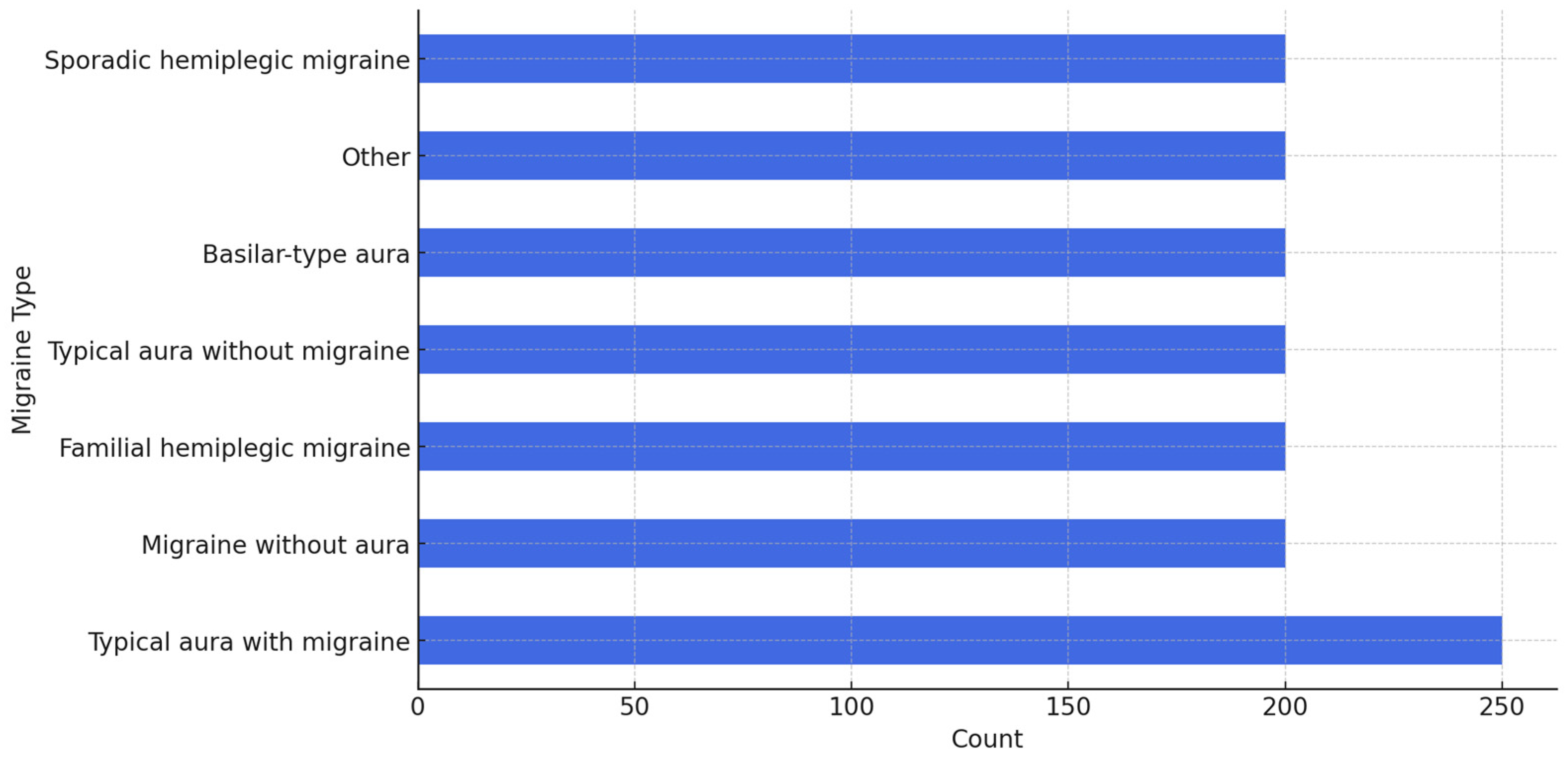
To deal with the imbalance in the dataset, we used an oversampling technique to sample up all migraine types to ensure the minority classes would not be ignored by the model. The oversampling was performed on the entire dataset. We sampled all the less common migraine types, up to 200 samples each, while leaving “typical aura with migraine” at 250 since it already had plenty of samples. Figure 3 shows a visualization of how the dataset looks after this up-sampling. By using this method, we balanced the dataset and allowed the model a fair chance at learning all the different migraine types.

Figure 3. The distribution of migraine types in the dataset (output classes) after up-sampling.

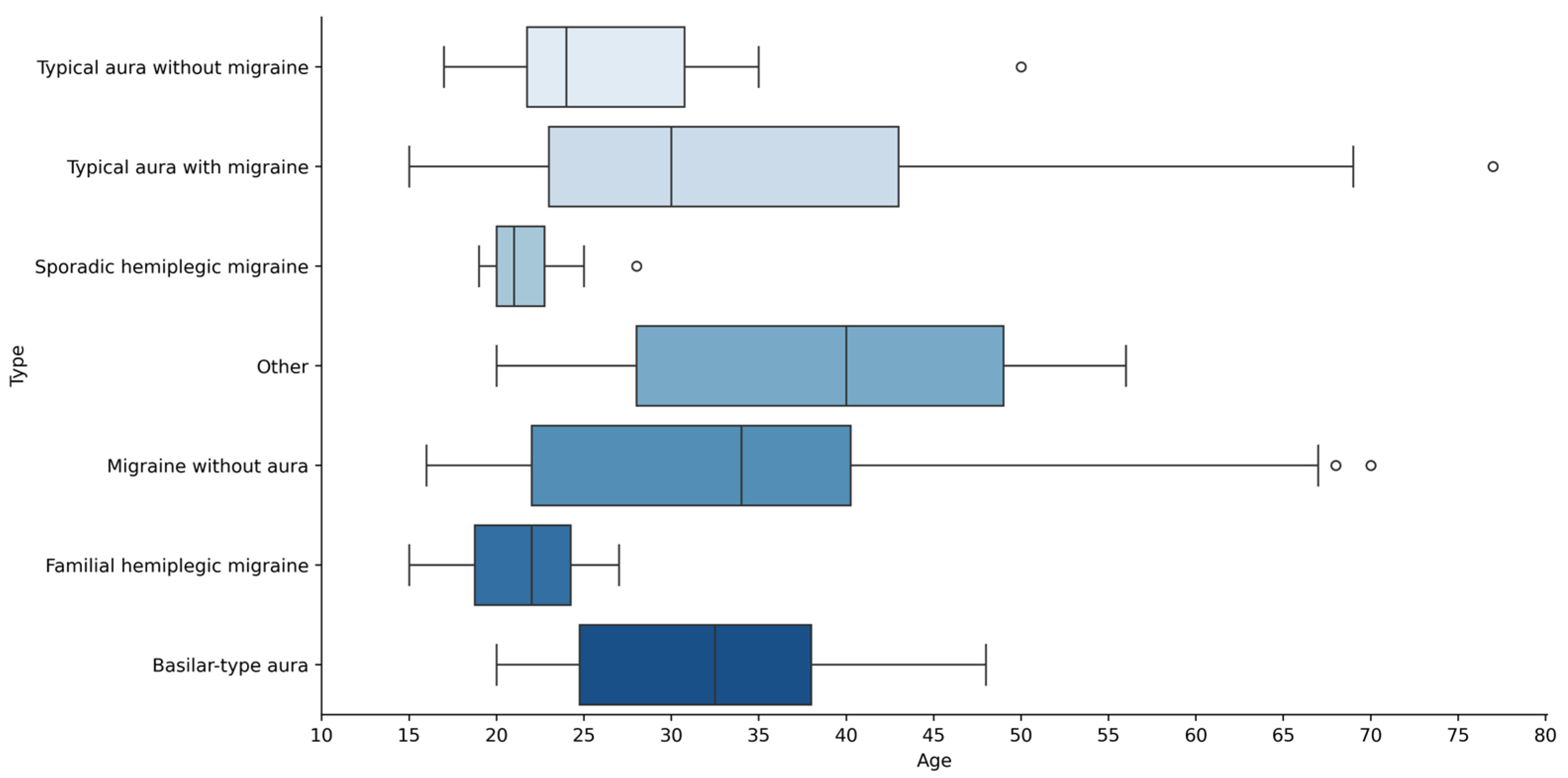
To check for unusual ages in the different type groups, we constructed a boxen plot as shown in Figure 4. This plot showed a few ages beyond the main range, which means there were some older people in the data sample. Using the interquartile range (IQR) method, four ages—28, 50, 68, 70, and 77—were detected as outliers. But since these ages are still within a reasonable range in studies about migraines, we did not eliminate them. By keeping these data points, we ensure that our study stays accurate and does not ignore how migraines affect older adults. Dropping those ages could have led to missing important insights or even skewing the results, especially since age is such a crucial factor here.

Figure 4. Age distribution across migraine types.

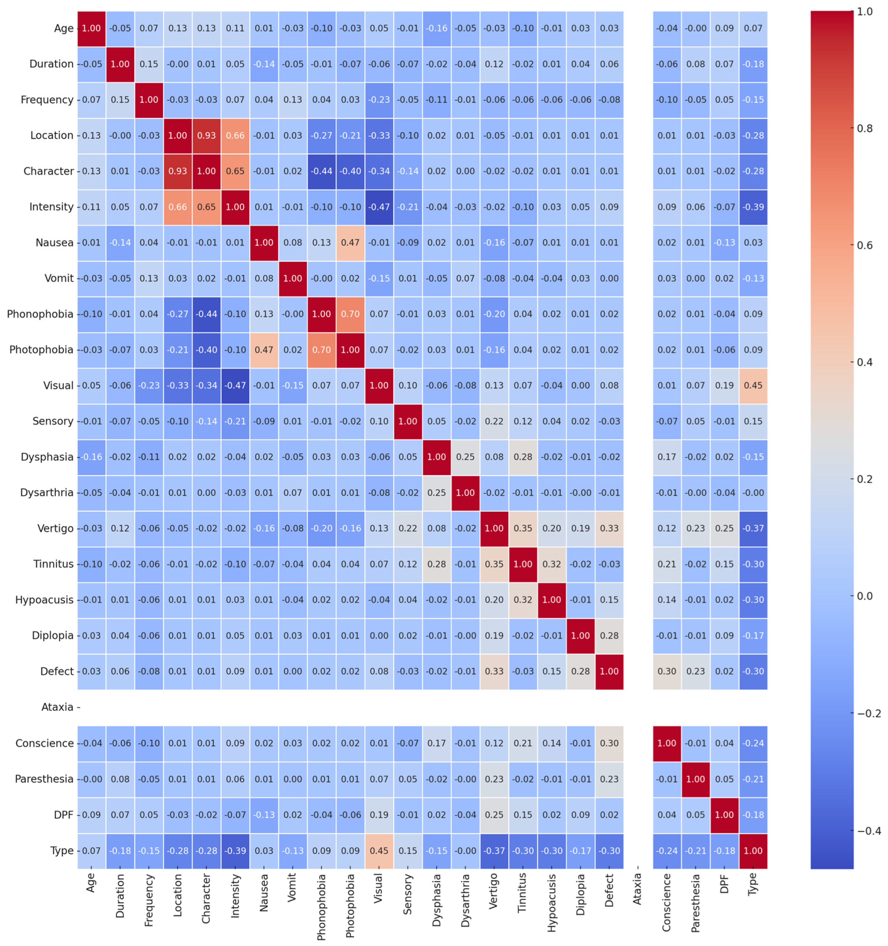
To check how the “Type” feature is related to other features, we performed a correlation analysis. This method is useful because it shows which features are important when trying to predict the “Type” feature. But since the “Type” feature was a categorical variable, we first converted it to a number using a one-hot encoding method. Then, we performed a Pearson correlation to assess how strongly the “Type” feature is linked with other features. The results, shown in Figure 5, indicated that some features had a strong positive or negative connection with the “Type” feature, while others did not seem connected at all. From Figure 5, it is obvious that the “Ataxia” feature had zero variance—every value was zero across the entire dataset. Because of that, it did not offer any useful information. So, we dropped it to only focus on features that could contribute meaningful information and help increase performance.

Figure 5. Correlation matrix across migraine types.

3.2. Machine Learning Classifiers

Artificial intelligence, or AI, is a branch of computer science that is all about teaching machines to think and act like humans. It is all about mimicking human skills, like learning, reasoning things out, and even recognizing and correcting mistakes. AI systems accomplish this by processing data repeatedly, so they can uncover hidden patterns without explicitly being programmed [14].

Machine learning, or ML, is a branch of AI that is focused on teaching computers to learn from data. It enables computers to learn information, figure out trends, and make decisions without human intervention [15]. This means that ML algorithms are not programmed to solve problems. Instead, they learn by analyzing data and figuring things out along the way [16]. There is a variety of ML techniques—some supervised, some unsupervised—that can be used to classify different types of migraines. Supervised learning is about teaching a model using past observations and their results, so it can learn to handle new observations. Unsupervised learning, on the other hand, does not rely on known results. It just tries to uncover hidden patterns and relationships by itself [17,18]. In the next sections, we will describe ML classifiers used for this study and how they work.

3.2.1. Decision Tree

The decision tree is basically one of the most popular algorithms for sorting data into categories or predicting numbers. It is like a flowchart where at each decision box (or node), the tree asks a question about the data and decides which path to go next. This keeps happening until it lands at a final decision. To determine which questions (or features) to ask at each node, a concept called entropy is used. Entropy is just a way of measuring how messy or unpredictable data are. If the data are messy, the entropy is high. If it is organized, the entropy is low. When the tree splits the data based on a certain feature, it checks if the data become clearer—meaning the entropy drops. The improvement in clarity is called information gain. So, the larger the information gain, the more that feature helps make accurate decisions. The tree is built by always picking the feature that provides the highest information gain. This keeps going until there are no good splits left (or all the features are basically used up) [19,20]. Given the following, dataset $D$, feature $Y$ in dataset $D$, probability ($p_i$) of class $i$, and subset ($D_y$) of dataset $D$ where feature $Y$ has a $C$ value and $values\left(Y\right)$ set of possible values for feature $Y$, the entropy $E\left(D\right)$ of the target variable and $Gain\left(D,Y\right)$ can be calculated as follows [20]:

$$E\left(D\right)=-\sum _{i=1}^{\left|C\right|}{p}_i{\mathit{log}}_2\left(p_i\right)$$

(1)

$$Gain\left(D,Y\right)=E\left(D\right)-\sum _{yϵvalues\left(Y\right)}{\displaystyle \frac{\left|D_y\right|}{\left|D\right|}}E\left(D_y\right)$$

(2)

In this paper, we trained the decision tree using a random splitter along with entropy to measure how good each split was. We also limited the depth of the tree to 10 splits. This is super important because it stops the tree from becoming too complicated and just memorizing the training data (which is called overfitting).

3.2.2. Naïve Bayes

The naïve Bayes is a simple but powerful algorithm that uses probability to make predictions. It is based on Bayes’ Theorem, and it assumes that each feature (or variable) within the same class is independent from the others [21]. This independence assumption helps naïve Bayes compute the probability of a class given some input data, even when dealing with complex combinations of features. That is one reason it handles high-dimensional data so well [22]. The naïve Bayes classifier is built on three key ideas. First, antecedent—basically, what happened in the past. Second, feasibility—how likely something is to happen in the future. Third, prediction—using antecedent and feasibility to predict what is coming next, as shown in Equation (3) [23]:

$$P\left(\left.C\right|X\right)={\displaystyle \frac{P\left(\left.X\right|C\right)\times \mathrm{P}\left(\mathrm{C}\right)}{P\left(\mathrm{X}\right)}}$$

(3)

where $C$ is the class label, $X$ is the observed feature, $P\left(\left.C\right|X\right)$ represents the prediction (the probability of class $C$ given feature $X$), $P\left(\left.X\right|C\right)$ represents the feasibility (the probability of feature $X$ given class $C$), $\mathrm{P}\left(\mathrm{C}\right)$ represents the antecedent (the prior probability of class $C$), and $P\left(X\right)$ represents the corroboration (the marginal probability of the observed feature $\mathrm{X}$ used for normalization).

In this paper, we used Gaussian naïve Bayes, which is a version of naïve Bayes that assumes data follow a normal (bell curve) distribution. Instead of just counting how often certain values occur (like in categorical naïve Bayes), it calculates how likely a feature value is. This makes it particularly good for continuous data [23].

3.2.3. K-Nearest Neighbor

The k-nearest neighbor is a powerful algorithm for both classification and regression tasks. It needs to have a labeled dataset—meaning the algorithm already knows what the correct outputs should be for the training data. A k-nearest neighbor classifies a new data point by checking how similar that point is to others it has seen before. But instead of looking at all the training data, it only focuses on the k closest ones—where k is the number of nearest neighbors. For example, if k = 8, the algorithm finds the eight data points that are nearest to the new data input. Then, it sees which class or label appears the most among those eight. That majority label becomes the prediction [24].

To decide which points are nearest, the algorithm computes the Euclidean distance. Basically, it measures the straight-line distance between two points. So, in a 2D space, if point $A$ is at (${\mathrm{x}}_1$, ${\mathrm{y}}_1$) and point $B$ is at (${\mathrm{x}}_2$, ${\mathrm{y}}_2$), the distance ($D$) between them is calculated using the following equation [23]:

$$D\left(A, B\right)=\sqrt{{\left({\mathrm{x}}_2-{\mathrm{x}}_1\right)}^2+{\left({\mathrm{y}}_2-{\mathrm{y}}_1\right)}^2}$$

(4)

This algorithm works well in practice, especially when the data are well structured and the features are on similar scales. But it can become tricky with high-dimensional data or when the features have very different ranges—so some pre-processing might be needed.

3.3. Ensemble Classifiers

Ensemble learning is a way of combining multiple machine learning (ML) models to achieve more accurate classifications. Instead of relying on a single ML model, which might not be too accurate, we combine the classification results from several models to achieve a stronger, more reliable classification. These models can all be of the same type (like several decision trees) or completely different (like a mix of SVMs, neural networks, etc.). The ensemble learning models are referred to as base models or weak learners, since they are not always great on their own but work better as a group [25,26,27]. In this paper, we used ensemble techniques to boost the performance of different ML models for migraine classification. In the following sections, we describe the strategy of the four ensemble classifiers used in this study.

3.3.1. Bagging

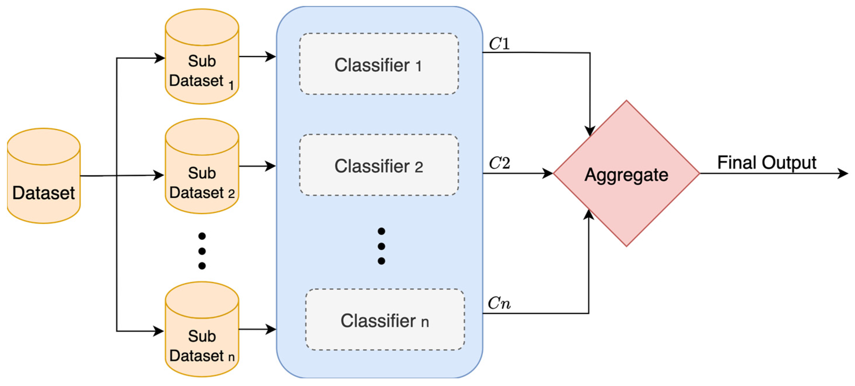
Bagging, or bootstrap aggregation, is an ensemble technique that trains multiple versions of the same classifier on different samples of the data, as shown in Figure 6. In this method, multiple subdatasets are created by randomly sampling from the training data with replacement. This means some points are picked more than once, and others might not be picked at all. Each of these subdatasets is called a bootstrap replicate. Also, several versions of the same classifier are built and trained separately on each subdataset. Once they are all trained, their outputs are combined. For regression, the outputs are just averaged. For classification, the majority vote from all classifiers is taken. This helps reduce variance in the final output and prevents classifiers from being thrown off by outliers in the data. Bagging works well when using classifiers that tend to overfit, like decision trees. However, if the data are noisy, bagging will not clean them up. It just helps smooth out random fluctuations, not actual mistakes. To calculate the final aggregated output $\widehat{\mathrm{y}}$, Equation (5) is used [28].

$$\widehat{\mathrm{y}}={\displaystyle \frac{1}{M}}\sum _{\mathrm{m}=1}^M{\mathrm{h}}_m\left(x\right)$$

(5)

where $M$ is the number of base classifiers, and ${\mathrm{h}}_m\left(x\right)$ is the classification output from classifier $m$.

Figure 6. The bagging ensemble architecture.

3.3.2. Majority Voting

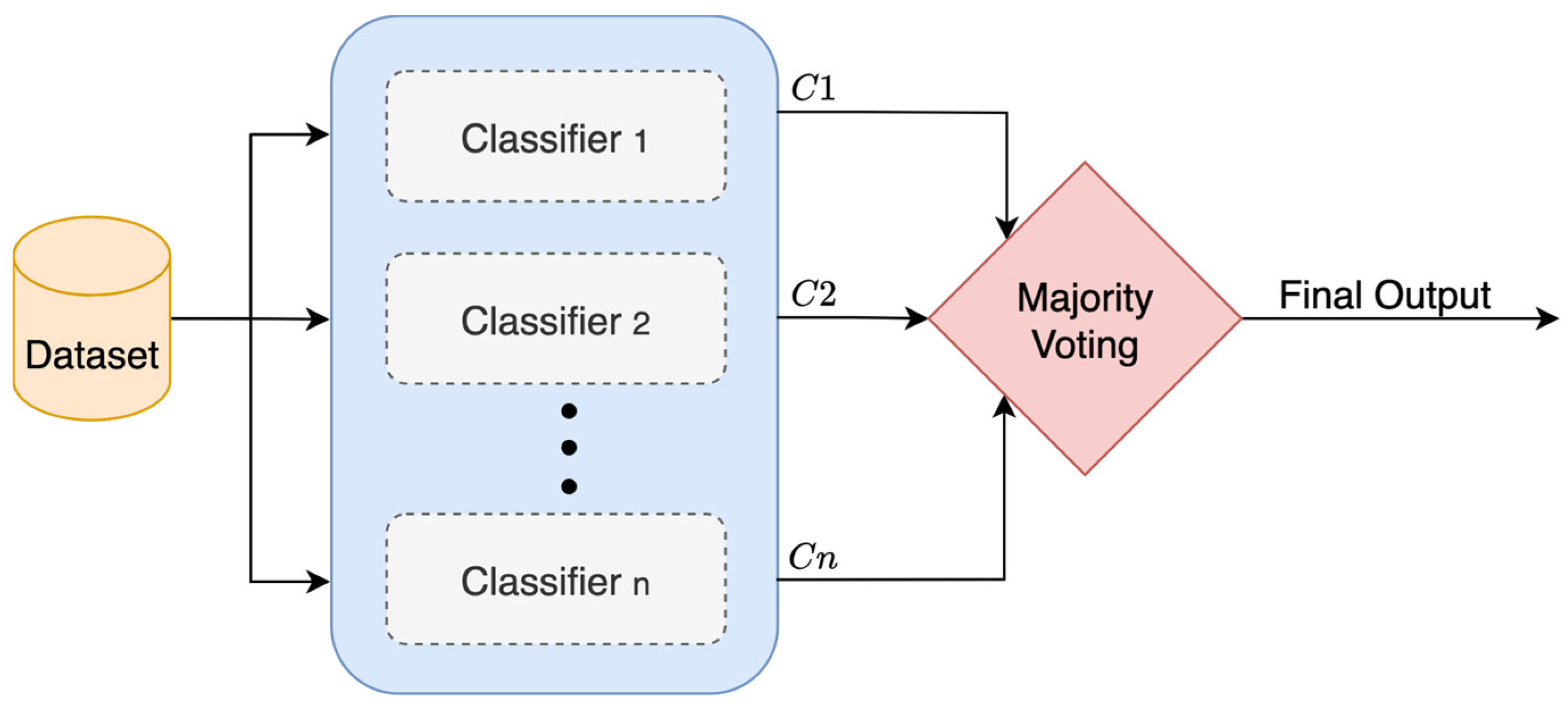
Voting is one of the simplest and most common ensemble methods in machine learning. It combines output from multiple classifiers and decides on the final output using a “voting” system, as shown in Figure 7. It uses either a hard voting or a soft voting mechanism. In hard voting, each base classifier selects a class label, and whichever class receives the most votes becomes the final output. For example, if three classifiers are used and two of them predict Class A while one predicts Class B, then the ensemble will go with Class A. In soft voting, the predicted probabilities from each base classifier are averaged for each class label. The class with the highest average probability becomes the final output [28,29].

Figure 7. The majority voting ensemble architecture.

All the base classifiers in a voting ensemble are trained separately using the same training data, and then their classifications are made on the same test data. One of the advantages of this approach is that it allows for diversity in the classifiers—meaning different types of classifiers can be used together, which often leads to better performance [30]. However, a voting ensemble does not always work well. If all the models are weak or very similar in how they make classifications, the benefits of combining them might be limited. To calculate the final output $\widehat{\mathrm{y}}$, Equation (6) is used [23].

$$\widehat{\mathrm{y}}=\mathrm{m}\mathrm{a}\mathrm{j}\mathrm{o}\mathrm{r}\mathrm{i}\mathrm{t}\mathrm{y}\_\mathrm{v}\mathrm{o}\mathrm{t}\mathrm{e}\left(h_1\right(x),h_2(x),\dots ,h_n(x\left)\right)$$

(6)

where $h_1\left(x\right),h_2\left(x\right),\dots ,h_n\left(x\right)$ are classification outputs of $n$ base classifiers.

3.3.3. Boosting

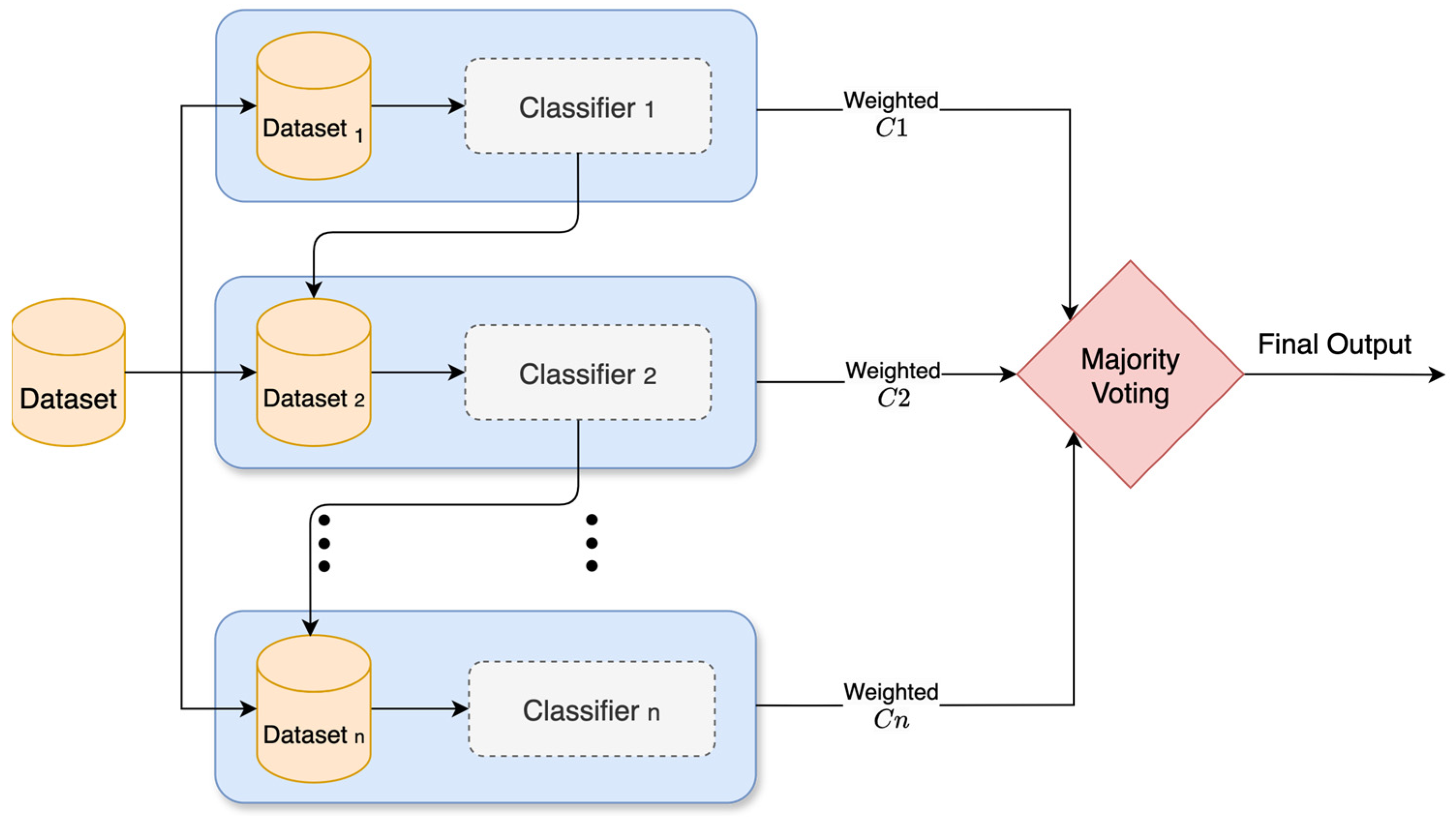
Boosting is an ensemble method that builds classifiers sequentially, as shown in Figure 8. It trains classifiers one after another, not all at once. Each new classifier tries to correct the mistakes made by the one before it. So, the overall system keeps improving. It is especially useful when data are unbalanced—when one output class has way more examples than the other. However, it can overfit and just memorize the training data instead of learning real patterns if the parameters are not tuned properly.

Figure 8. The boosting ensemble architecture.

Instead of training one larger classifier, boosting trains a bunch of smaller, simpler ones—these are called “weak learners”. At first, these classifiers might not perform that well. But after each round, the algorithm focuses more on the misclassified data. It creates new subsets of the data where those misclassified data are highlighted and trains the next classifier on that.

Eventually, all these weak classifiers are combined into one powerful classifier, usually by a cost function—basically a way to measure how far off the classifications are. To calculate the final weighted vote output $\widehat{\mathrm{y}}$ for binary classification, Equation (7) is used [28].

$$\widehat{\mathrm{y}}=\mathrm{s}\mathrm{i}\mathrm{g}\mathrm{n}\left(\sum _{\mathrm{m}=1}^M{{\mathsf{\alpha }}_m\mathrm{h}}_m\left(x\right)\right)$$

(7)

where ${\mathsf{\alpha }}_m$ is the weight assigned to classifier $m$ based on its accuracy, and ${\mathrm{h}}_m\left(x\right)$ is the classification output from classifier $m$.

3.3.4. Stacking

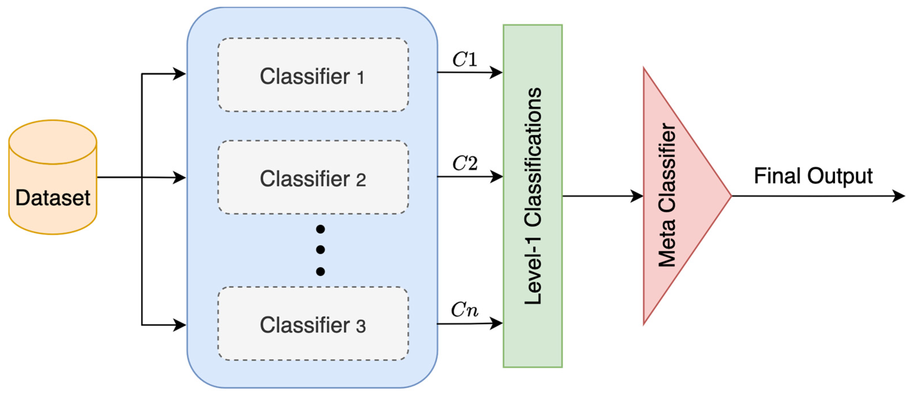
Stacking is an advanced ensemble learning method. It layers classifiers so that their outputs are fed into a meta-classifier, which makes the final output, as shown in Figure 9. It starts by training a few base classifiers on the same training data. Once they are trained, each one makes its own classification on the test data. Then, instead of just choosing one of those classifications, it gathers them all up and uses them as new input for the meta-classifier. To calculate the final output $\widehat{\mathrm{y}}$, Equation (8) is used [20].

$$\widehat{\mathrm{y}}=M \left(h_1\right(x),h_2(x),\dots ,h_n(x\left)\right)$$

(8)

where $M$ is a meta-classifier trained on classification outputs $h_1\left(x\right),h_2\left(x\right),\dots ,h_n\left(x\right)$ of n base classifiers.

Figure 9. The Stacking ensemble architecture.

This method usually boosts the overall performance because the meta-classifier can fix some of the mistakes made by the base classifiers. However, the architecture is not simple; it takes more time to train because it works with multiple classifiers stacked on top of each other.

3.4. Evaluation Metrics

To evaluate migraine classifiers, four parameters are looked at: (1) true negative (${\mathrm{T}}_{\mathrm{N}}$), indicating correct classification of healthy persons, (2) true positive (${\mathrm{T}}_{\mathrm{P}}$), indicating correct classification of diseased persons, (3) false positive (${ \mathrm{F}}_{\mathrm{P}}$), indicating incorrect classification of healthy persons, and (4) false negative (${\mathrm{F}}_{\mathrm{N}}$), indicating incorrect classification of diseased persons [31,32].

To measure the overall performance of all classifiers, we used the following metrics:

Accuracy, which focuses on how good the classifier is at correctly identifying both healthy and diseased people. It is calculated as follows:

$$\mathrm{Accuracy}={\displaystyle \frac{{\mathrm{T}}_{\mathrm{P}} + {\mathrm{T}}_{\mathrm{N}}}{{\mathrm{T}}_{\mathrm{P}} + {\mathrm{T}}_{\mathrm{N}} +{ \mathrm{F}}_{\mathrm{P}} + {\mathrm{F}}_{\mathrm{N}}}}$$

(9)

Precision, which focuses on how good the classifier is at correctly identifying healthy people. So, it is calculated using Equation (10) by dividing ${\mathrm{T}}_{\mathrm{N}}$ by all the people the classifier labeled as healthy.

$$\mathrm{Precision}={\displaystyle \frac{{\mathrm{T}}_{\mathrm{P}}}{{\mathrm{T}}_{\mathrm{N}}+{\mathrm{F}}_{\mathrm{P}}}}$$

(10)

Recall, which focuses on how good the classifier is at correctly identifying people who have migraines. So, it is calculated using Equation (11) by dividing ${\mathrm{T}}_{\mathrm{P}}$ by all the real migraine cases.

$$\mathrm{Recall}={\displaystyle \frac{{\mathrm{T}}_{\mathrm{P}}}{{\mathrm{T}}_{\mathrm{P}}+{\mathrm{F}}_{\mathrm{N}}}}$$

(11)

F1-Score, which combines precision and recall, as shown in Equation (12). It is helpful to balance between the two.

$$\mathrm{F}1\text{-}\mathrm{Score}=2{\displaystyle \frac{Recall\times Precision}{\mathrm{Recall}+\mathrm{Precision}}}$$

(12)

4. Results and Discussion

4.1. Performance of the Standalone Machine Learning Classifiers

In this section, we discuss the performance evaluation of the three standalone machine learning (ML) classifiers: decision tree (DT), naïve Bayes (NB), and k-nearest neighbors (KNN). After splitting the migraine dataset into train and test sets using an 80:20 split ratio, the three base classifiers were trained. We used a single 80:20 split because our dataset was small, and we wanted to ensure a completely untouched test set that reflects the classifiers’ performance on unseen data. During all training processes, the test set was kept out and not used. This separate test set was set aside specifically for the performance evaluation of base classifiers. After performing a comparative analysis of these classifiers’ performance, some classifiers showed good accuracy, whereas others performed poorly.

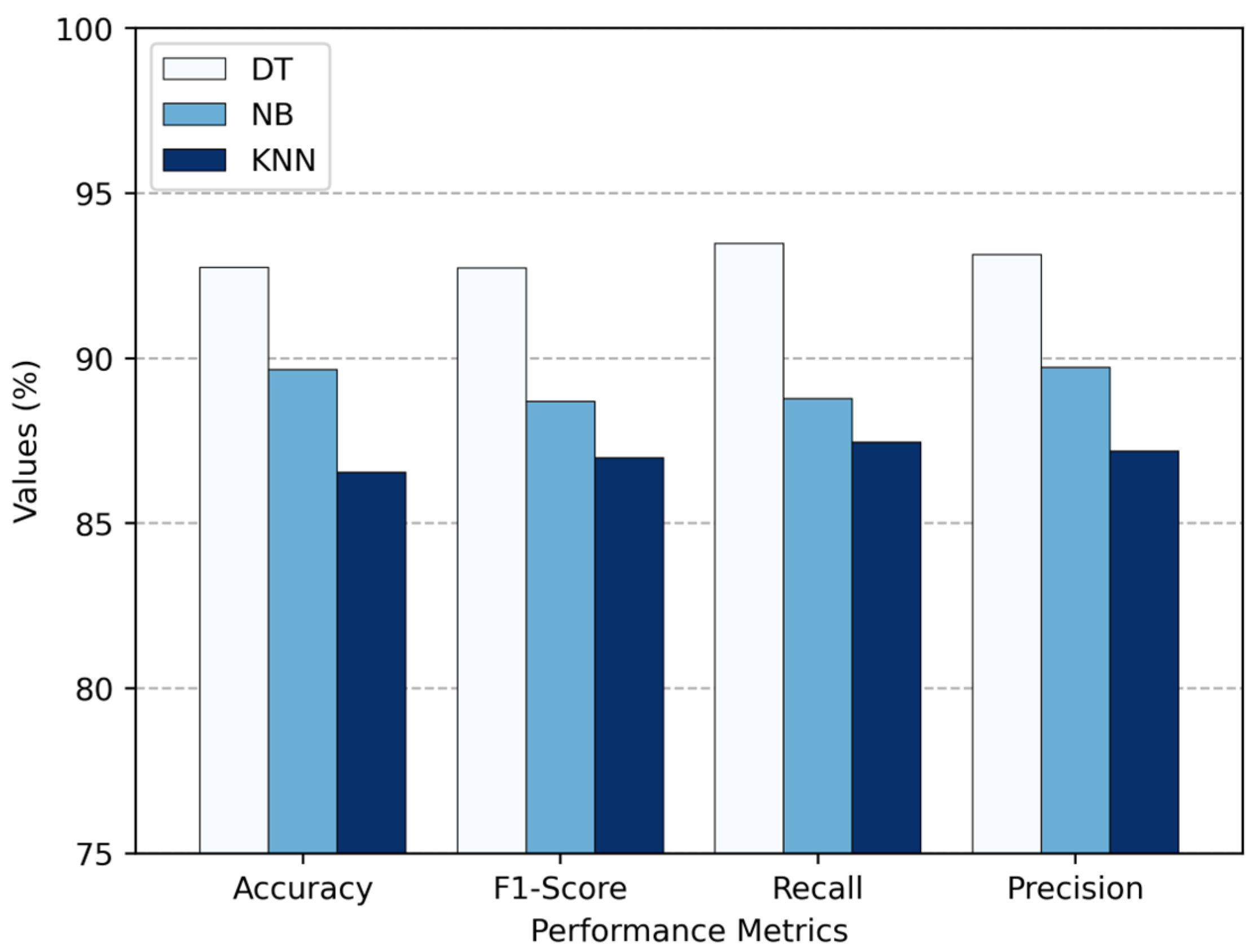
Table 3 shows the evaluation results of the three classifiers. The DT classifier outperformed the others with the highest accuracy of 92.76%. It also had the best scores for precision (93.14%), recall (93.48%), and f1-score (92.73%), which means it classified the different migraine types accurately and consistently. NB also performed well, despite missing a few more true cases than DT. Its accuracy was 89.66%, precision 89.73%, recall 88.78%, and f1-score 88.70%. Overall, NB was a dependable classifier, especially since it is based on probabilities and tends to be fast and simple. KNN, on the other hand, struggled a bit. It had the lowest accuracy (86.55%), precision (87.19%), recall (87.47%), and f1-score (86.99%), which suggests it did not handle the data that well. That is probably because KNN can be quite sensitive to how the data are scaled or spread out. So, in the end, DT came out as the top performer among the standalone classifiers for classifying migraine types.

Table 3. Performance metrics of standalone classifiers.

Classifier	Accuracy	Precision	Recall	F1-Score	Computation Time
DT	92.76%	93.14%	93.48%	92.73%	4.101 ms
NB	89.66%	89.73%	88.78%	88.70%	3.713 ms
KNN	86.55%	87.19%	87.47%	86.99%	2.673 ms

Figure 10 provides a clear visual that supports the numerical results in Table 3. It puts the results into a chart so that it is easier to compare how DT, NB, and KNN perform against each other. The comparison is based on key performance measures: accuracy, f1-score, recall, and precision. From the chart, it is clear that DT outperforms the other two.

Figure 10. Comparative performance of DT, NB, and KNN classifiers across evaluation metrics.

Table 3 does not just compare accuracy; it also shows how fast each classifier processes data. This shows how efficient they are when it comes to making classifications. KNN is the fastest, with a processing time of just 2.673 ms. That is kind of expected since KNN mostly relies on straightforward distance calculations, especially when the dataset size is moderate. NB comes next with 3.713 ms. It is also considered fast, because its calculations are based on simple probability rules. On the other hand, the DT, while the most accurate, takes the longest processing time of 4.101 ms. This extra time likely comes from the way DT works—by moving through multiple branches to reach a decision, which can become a bit heavy, especially with deeper trees. Overall, there is a clear trade-off between classifier complexity and computational efficiency: DT offers better classification accuracy, but KNN and NB are more efficient in terms of speed.

4.2. Performance of the Ensemble Classifiers

In this section, the classification performance of standalone ML classifiers was enhanced by using four ensemble methods: bagging, boosting, majority voting, and stacking. All four ensemble classifiers were built by combining DT, NB, and KNN classifiers. For boosting, we used the AdaBoost algorithm with 16 estimators. The stacking classifier had logistic regression as the meta-classifier. For voting, we used the hard voting approach. Finally, in bagging, we used 350 estimators for KNN and 100 each for NB and DT. After evaluating base classifiers with the test set, DT performed the best, while KNN and NB performed the worst. Likewise, the training set was used to train the ensemble classifiers, and the test set was used to evaluate them. The evaluation was based on accuracy, precision, recall, and f1-score.

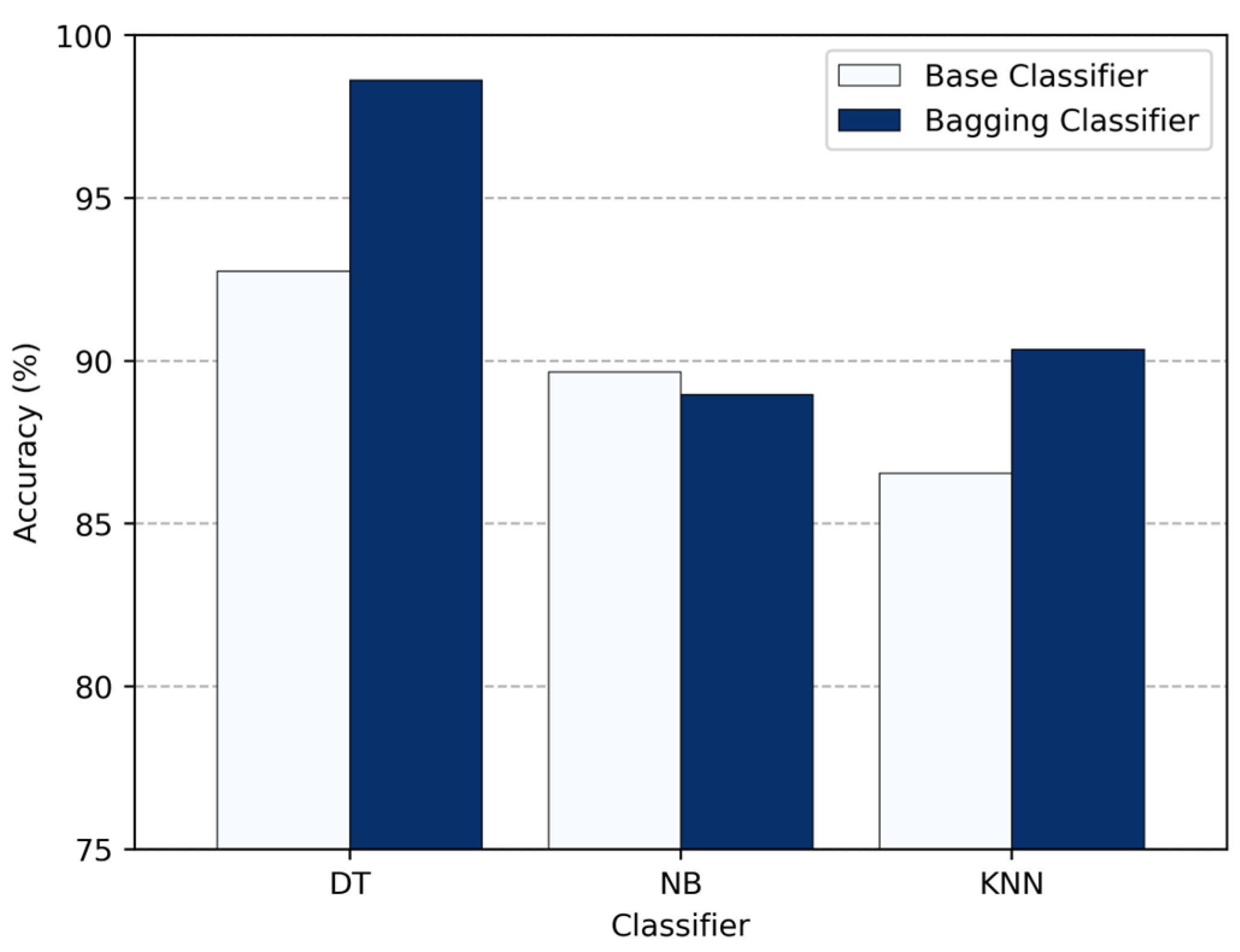
In Figure 11, we compare the accuracy of standalone classifiers—DT, NB, and KNN—with their bagging versions. On their own, DT achieved about 92.76%, NB about 89.66%, and KNN approximately 86.55%. After applying bagging, DT showed a large improvement to about 98.62%, and KNN to approximately 90.34%. NB, on the other hand, dropped slightly to 88.97%, showing that bagging does not achieve much for stable, low-variance classifiers like NB. These results make it clear that bagging is most helpful for high-variance classifiers like DT, providing them up to a 5.86% boost in accuracy, while its effect on stable classifiers is limited or even negative.

Figure 11. Improvement in accuracy of standalone classifiers with bagging ensemble.

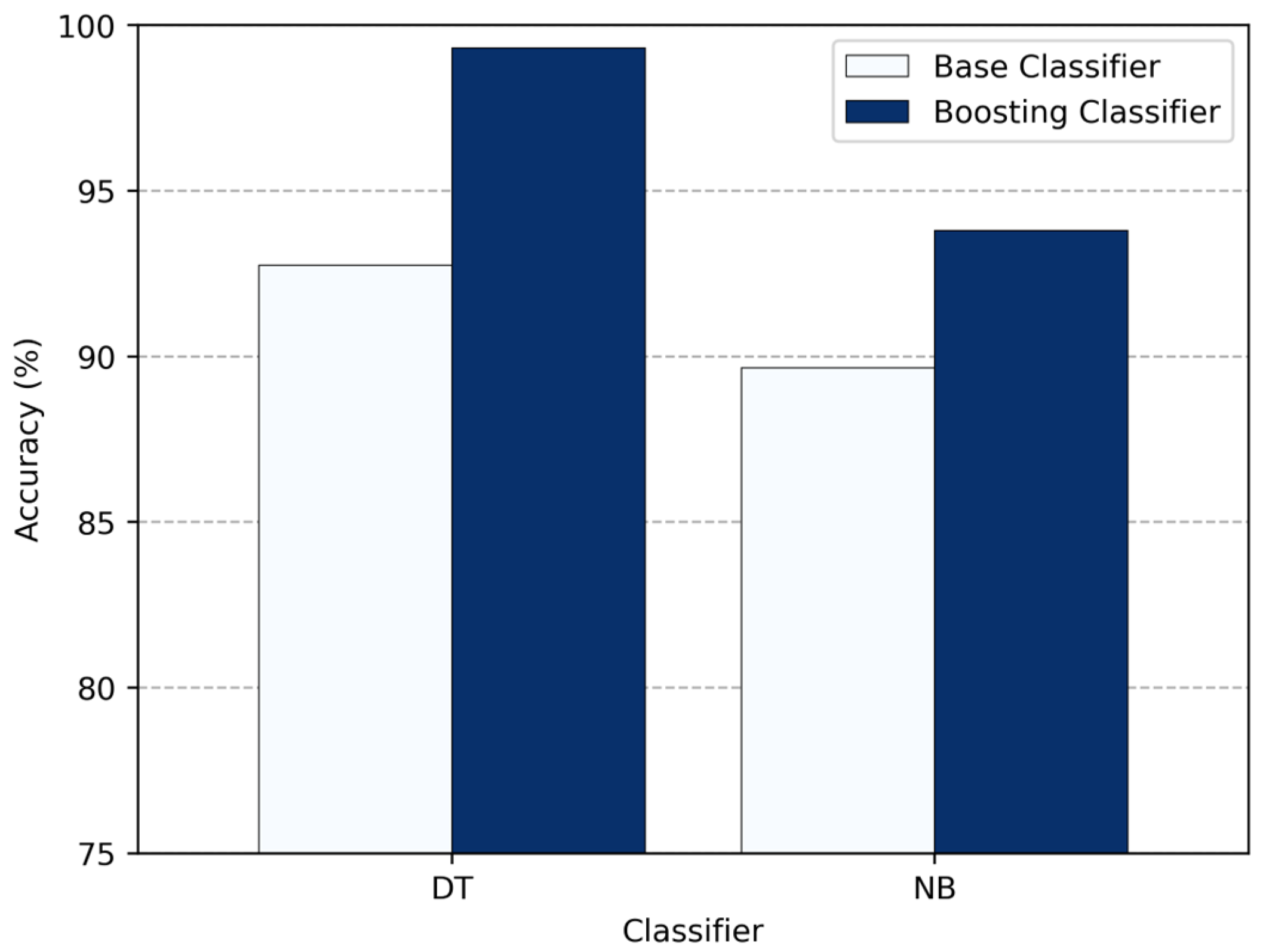
Next, in Figure 12, we compare how the standalone classifiers perform versus when boosting is applied. DT benefited the most—its accuracy increased by 6.55%, reaching about 99.31%. NB accuracy also improved to 93.79% (roughly 4.13% higher). KNN, however, is not compatible with boosting, so its performance did not change at all. Overall, these results show that boosting is extremely effective for high-bias classifiers like DT and provides a noticeable accuracy boost to NB, while KNN receives no effect.

Figure 12. Improvement in accuracy of standalone classifiers with boosting ensemble.

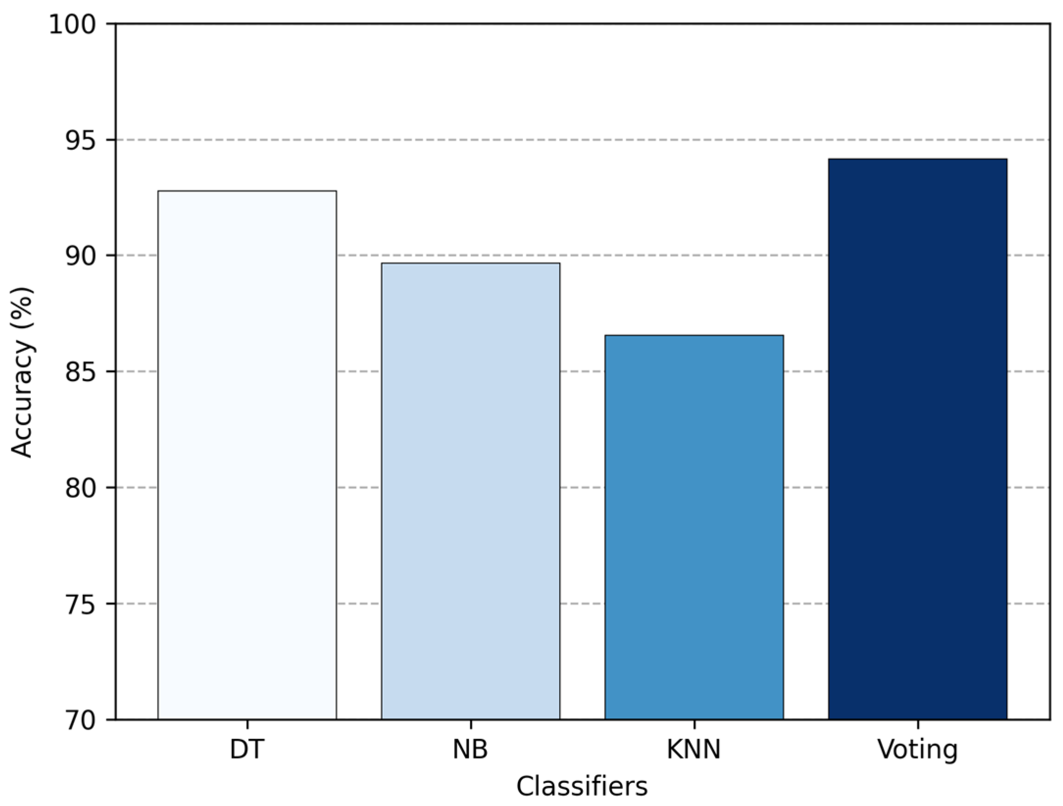
Then, in Figure 13, we compare the standalone classifiers with the ensemble created using majority voting. The voting approach boosted the overall accuracy up to 94.14%, which is higher than any of the single classifiers. This means it performed 1.38% better than DT, 4.48% better than NB, and 7.59% better than KNN. While the improvement is not huge, it is consistent. Voting works because it blends the strengths of multiple classifiers, providing a more reliable performance than any single classifier could on its own.

Figure 13. Improvement in accuracy of standalone classifiers with majority voting ensemble.

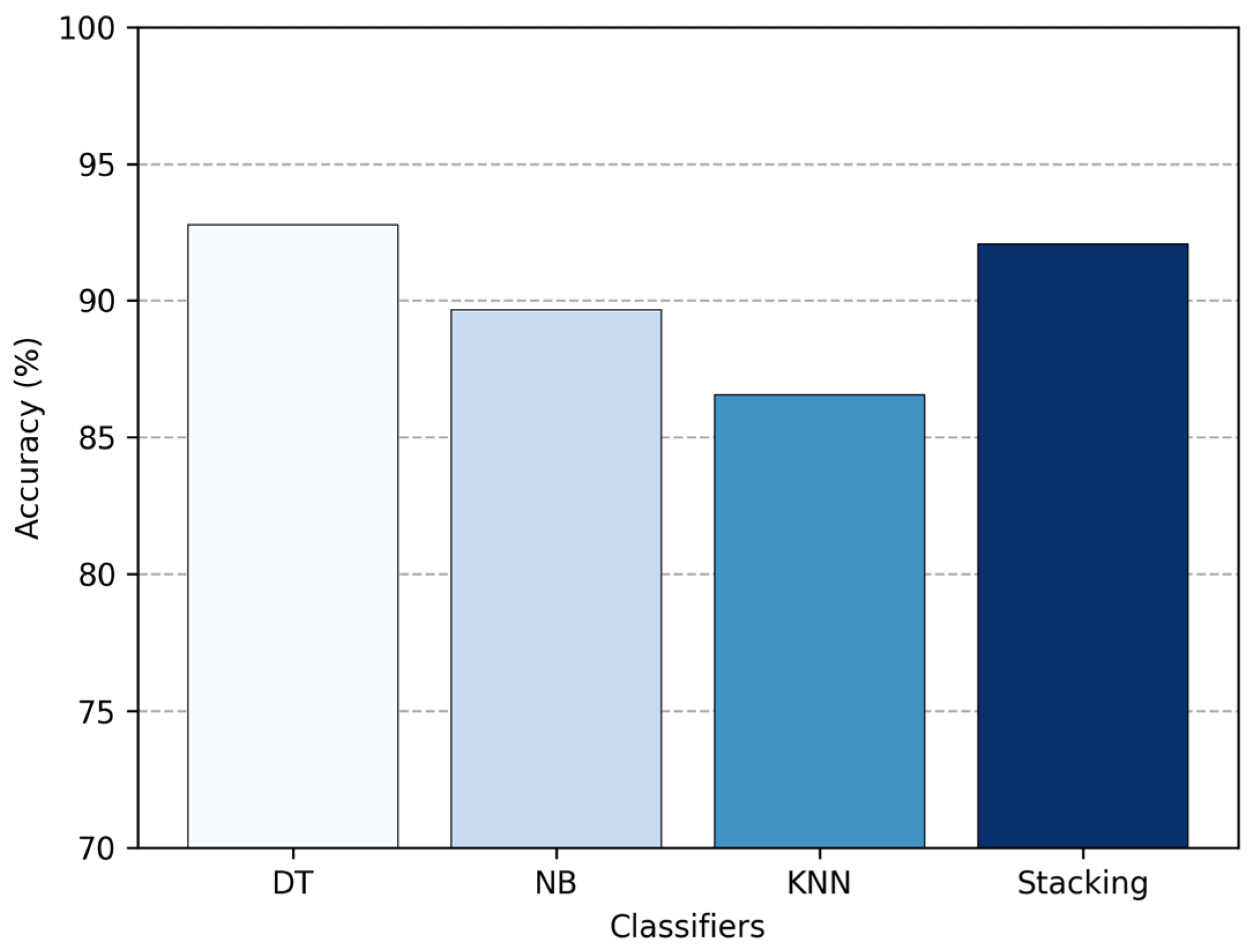
Similarly, in Figure 14, we compare the accuracy of the standalone classifiers with the stacking ensemble approach. Using stacking improved overall accuracy up to 92.07%, which is 2.41% higher than NB and 5.52% higher than KNN. However, it still came in slightly below DT, with about 0.69% lower accuracy. This shows that stacking can effectively boost the performance of weaker classifiers by combining their strengths, but in this case, it was not quite enough to outperform the strongest individual classifier, the DT.

Figure 14. Improvement in accuracy of standalone classifiers with stacking ensemble.

Finally, Table 4 summarizes the performance of all standalone and ensemble classifiers. The ensemble methods generally outperformed the standalone classifiers. Boosting DT was by far the best performer, achieving 99.31% accuracy and a 99.25% f1-score, which shows how well it balances precision and recall. Bagging DT also performed well with 98.62% accuracy. Majority voting and stacking provided some improvements over the standalone classifiers, but not as boosting or bagging. Overall, the results show that using ensembles, especially boosting, really enhances classification performance and makes the results more reliable.

Table 4. Comparison of performance metrics of standalone classifiers and ensemble classifiers.

Classifier	Accuracy	Precision	Recall	F1-Score
DT	92.76%	93.14%	93.48%	92.73%
NB	89.66%	89.73%	88.78%	88.70%
KNN	86.55%	87.19%	87.47%	86.99%
Majority Voting	94.14%	94.34%	94.43%	94.17%
Stacking	92.07%	91.90%	92.39%	91.69%
Bagging DT	98.62%	98.32%	98.70%	98.45%
Bagging NB	88.97%	89.24%	87.86%	87.94%
Bagging KNN	90.34%	90.25%	90.75%	90.14%
Boosting DT	99.31%	99.18%	99.35%	99.25%
Boosting NB	93.79%	93.71%	94.52%	93.53%

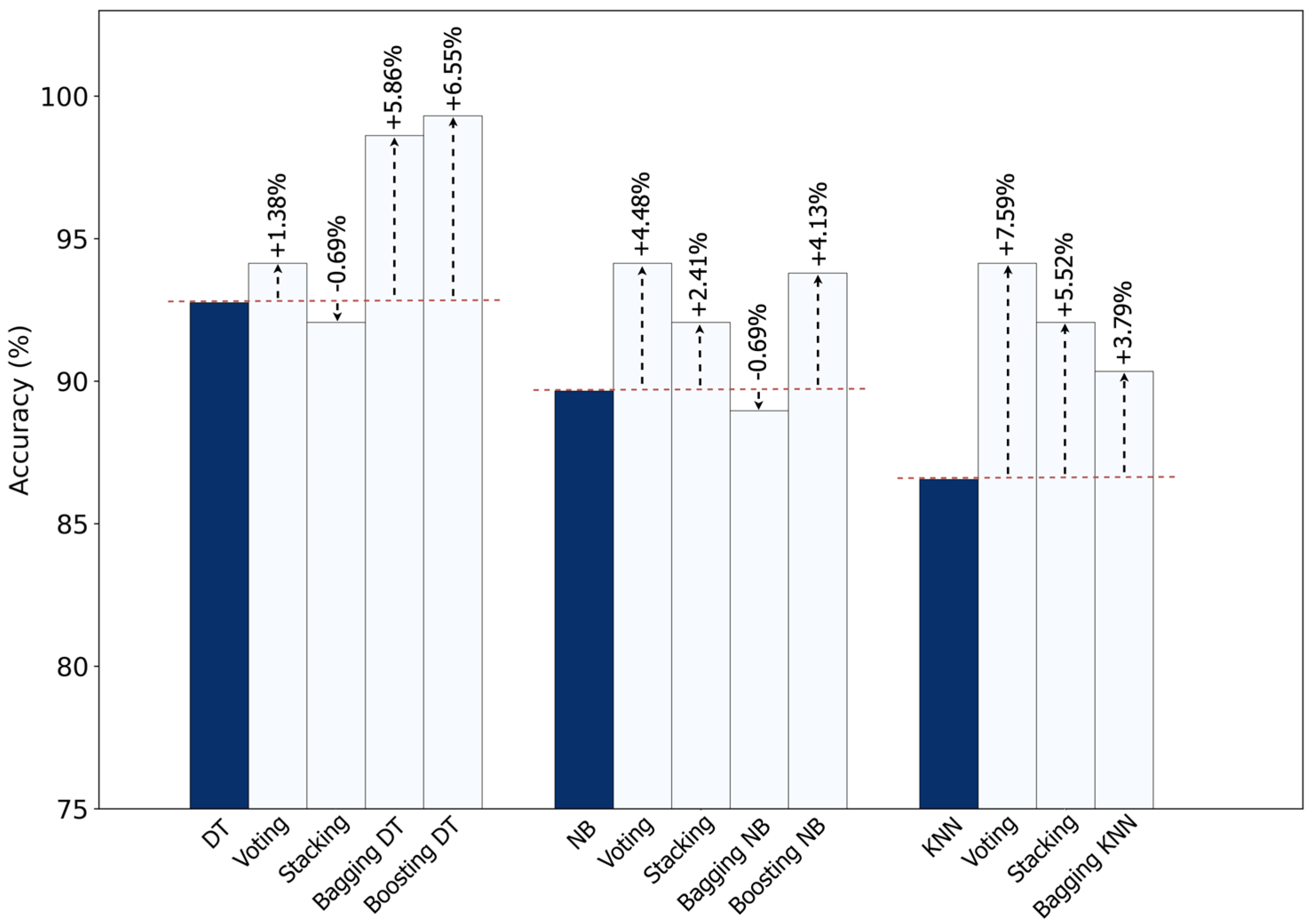
Comparing the different ensemble methods shows that the accuracy of standalone classifiers could be increased. Figure 15 highlights which ensemble approach provided the largest improvement for each base classifier. DT achieved the largest improvement from boosting, with a +6.55% gain. NB, on the other hand, performed best with voting, improving by +4.48%. Also, KNN achieved the highest overall boost—7.59%—also from voting. So overall, ensembles clearly make standalone classifiers stronger. Boosting is more suitable for DT, while voting consistently helps NB and KNN the most.

Figure 15. Improvement in accuracy of standalone classifiers using different ensemble methods.

Even though real-time classification of migraines is not critical for clinical application, we measured the computation time of each classifier to further evaluate the efficiency. Table 5 compares the runtime of the standalone classifiers versus their ensemble versions. The table shows that standalone classifiers are faster: KNN only takes 2.673 ms, NB takes 3.713 ms, and DT takes 4.101 ms. While with ensemble methods, the runtime increases since they are combining multiple classifiers. Voting ensemble adds just a small delay at about 8.191 ms. Stacking, though, is extremely slow—over a full second (1095.617 ms)—because of all the extra meta-learning involved. Bagging falls in the middle, taking approximately 297.793 ms for DT, 370.798 ms for NB, and 556.684 ms for KNN. Boosting is relatively quick, with 36.113 ms for NB and 44.632 ms for DT, although KNN can not be boosted. Overall, ensemble methods provide better classification accuracy but cost more time, and stacking is by far the slowest approach.

Table 5. Comparison of computation time of standalone classifiers and ensemble classifiers.

Classifier	Without Ensemble	With Voting	With Stacking	With Bagging	With Boosting
DT	4.101 ms	8.191 ms	1095.617 ms	297.793 ms	44.632 ms
NB	3.713 ms			370.798 ms	36.113 ms
KNN	2.673 ms			556.684 ms	-

5. Conclusions

This paper examines how well individual machine learning (ML) classifiers perform compared to ensemble classifiers when classifying different types of migraines. Using a structured migraine dataset, we trained three ML classifiers: decision tree (DT), naïve Bayes (NB), and k-nearest neighbor (KNN). Before training, the dataset was cleaned and balanced by using pre-processing and oversampling.

Among the individual classifiers, DT achieved the highest accuracy (92.76%), followed by NB (89.66%) and KNN (86.55%). We also investigated ensemble techniques like bagging, boosting, stacking, and majority voting to enhance the performance of standalone classifiers. The results showed that majority voting provided the largest accuracy improvement (7.59%), with boosting, bagging, and stacking following behind at 6.55%, 5.86%, and 5.52% improvements, respectively.

These results highlight that ML—especially ensemble methods—can be a powerful, cost-effective way to classify migraines. Instead of relying only on subjective evaluations or expensive tests, these ML methods can help support quicker and more personalized treatment plans, which are especially useful for clinics with limited resources.

Despite these promising results, the study has its limitations. The study only used one publicly available dataset, and it only focused on migraine classification. So, the models’ generalizability to broader populations with varied demographic or medical histories remains to be validated. For future research, it would be great to explore the proposed framework with real clinical data, explore other medical conditions, and even include multimodal data like EEG signals or data from wearable devices. This would make the framework more robust and clinically applicable in the real world.

References

- Galvez-Goicurla, J.; Pagan, J.; Gago-Veiga, A.B.; Moya, J.M.; Ayala, J.L. Cluster-Then-Classify Methodology for the Identification of Pain Episodes in Chronic Diseases. IEEE J. Biomed. Health Inform. 2022, 26, 2339–2350. [Google Scholar] [CrossRef] [PubMed]
- Hsiao, F.J.; Chen, W.T.; Wu, Y.T.; Pan, L.L.H.; Wang, Y.F.; Chen, S.P.; Lai, K.L.; Coppola, G.; Wang, S.J. Characteristic oscillatory brain networks for predicting patients with chronic migraine. J. Headache Pain. 2023, 24, 139. [Google Scholar] [CrossRef]
- Chen, W.T.; Hsieh, C.Y.; Liu, Y.H.; Cheong, P.L.; Wang, Y.M.; Sun, C.W. Migraine classification by machine learning with functional near-infrared spectroscopy during the mental arithmetic task. Sci. Rep. 2022, 12, 14590. [Google Scholar] [CrossRef]
- Chong, C.D.; Gaw, N.; Fu, Y.; Li, J.; Wu, T.; Schwedt, T.J. Migraine classification using magnetic resonance imaging resting-state functional connectivity data. Cephalalgia 2017, 37, 828–844. [Google Scholar] [CrossRef]
- Zhu, B.; Coppola, G.; Shoaran, M. Migraine classification using somatosensory evoked potentials. Cephalalgia 2019, 39, 1143–1155. [Google Scholar] [CrossRef]
- Ko, H.K. Applying Machine Learning models to Diagnosing Migraines with EEG Diverse Algorithms. J. Mach. Comput. 2024, 4, 170–180. [Google Scholar] [CrossRef]
- Hsiao, F.J.; Chen, W.T.; Pan, L.L.H.; Liu, H.Y.; Wang, Y.F.; Chen, S.P.; Lai, K.L.; Coppola, G.; Wang, S.J. Resting-state magnetoencephalographic oscillatory connectivity to identify patients with chronic migraine using machine learning. J. Headache Pain. 2022, 23, 130. [Google Scholar] [CrossRef] [PubMed]
- Abed, R.A.; Hamza, E.K.; Humaidi, A.J. A modified CNN-IDS model for enhancing the efficacy of intrusion detection system. Meas. Sens. 2024, 35, 101299. [Google Scholar] [CrossRef]
- Mansoor, M.I.; Tuama, H.M.; Humaidi, A.J. Application of correlation-based recurrent neural network in porosity prediction for petroleum exploration. Eng. Res. Express 2025, 7, 015241. [Google Scholar] [CrossRef]
- Krawczyk, B.; Simić, D.; Simić, S.; Woźniak, M. Automatic diagnosis of primary headaches by machine learning methods. Cent. Eur. J. Med. 2013, 8, 157–165. [Google Scholar] [CrossRef]
- Frid, A.; Shor, M.; Shifrin, A.; Yarnitsky, D.; Granovsky, Y. A Biomarker for Discriminating Between Migraine with and Without Aura: Machine Learning on Functional Connectivity on Resting-State EEGs. Ann. Biomed. Eng. 2020, 48, 403–412. [Google Scholar] [CrossRef] [PubMed]
- Hsiao, F.J.; Chen, W.T.; Wang, Y.F.; Chen, S.P.; Lai, K.L.; Coppola, G.; Wang, S.J. Identification of patients with chronic migraine by using sensory-evoked oscillations from the electroencephalogram classifier. Cephalalgia 2023, 43, 1–11. [Google Scholar] [CrossRef]
- Sanchez-Sanchez, P.A.; García-González, J.R.; Ascar, J.M.R. Automatic migraine classification using artificial neural networks. F1000Research 2020, 9, 618. [Google Scholar] [CrossRef]
- Yang, H.; Li, Z.; Wang, Z. Prediction of atherosclerosis diseases using biosensor-assisted deep learning artificial neuron model. Neural Comput. Appl. 2021, 33, 5257–5266. [Google Scholar] [CrossRef]
- Nisar, D.E.M.; Amin, R.; Shah, N.U.H.; Ghamdi, M.A.A.; Almotiri, S.H.; Alruily, M. Healthcare Techniques Through Deep Learning: Issues, Challenges and Opportunities. IEEE Access 2021, 9, 98523–98541. [Google Scholar] [CrossRef]
- Sevakula, R.K.; Au-Yeung, W.M.; Singh, J.P.; Heist, E.K.; Isselbacher, E.M.; Armoundas, A.A. State-of-the-Art Machine Learning Techniques Aiming to Improve Patient Outcomes Pertaining to the Cardiovascular System. J. Am. Heart Assoc. 2020, 9, e013924. [Google Scholar] [CrossRef] [PubMed]
- Mathur, P.; Srivastava, S.; Xu, X.; Mehta, J.L. Artificial Intelligence, Machine Learning, and Cardiovascular Disease. Clin. Med. Insights Cardiol. 2020, 14, 1–9. [Google Scholar] [CrossRef] [PubMed]
- Samaan, S.S.; Korial, A.E.; Sarra, R.R.; Humaidi, A.J. Multilingual web traffic forecasting for network management using artificial intelligence techniques. Results Eng. 2025, 26, 105262. [Google Scholar] [CrossRef]
- Kapila, R.; Ragunathan, T.; Saleti, S.; Lakshmi, T.J.; Ahmad, M.W. Heart Disease Prediction using Novel Quine McCluskey Binary Classifier (QMBC). IEEE Access 2023, 11, 64324–64347. [Google Scholar] [CrossRef]
- Sarra, R.R.; Gorial, I.I.; Manea, R.R.; Korial, A.E.; Mohammed, M.; Ahmed, Y. Enhanced Stacked Ensemble-Based Heart Disease Prediction with Chi-Square Feature Selection Method. J. Robot. Control (JRC) 2024, 5, 1753–1763. [Google Scholar]
- Gao, X.-Y.; Amin Ali, A.; Shaban Hassan, H.; Anwar, E.M. Improving the accuracy for analyzing heart diseases prediction based on the ensemble method. Complexity 2021, 2021, 6663455. [Google Scholar] [CrossRef]
- Tiwari, A.; Chugh, A.; Sharma, A. Ensemble framework for cardiovascular disease prediction. Comput. Biol. Med. 2022, 146, 105624. [Google Scholar] [CrossRef]
- Korial, A.E.; Gorial, I.I.; Humaidi, A.J. An Improved Ensemble-Based Cardiovascular Disease Detection System with Chi-Square Feature Selection. Computers 2024, 13, 126. [Google Scholar] [CrossRef]
- Du, Z.; Yang, Y.; Zheng, J.; Li, Q.; Lin, D.; Li, Y.; Fan, J.; Cheng, W.; Chen, X.-H.; Cai, Y. Accurate prediction of coronary heart disease for patients with hypertension from electronic health records with big data and machine-learning methods: Model development and performance evaluation. JMIR Med. Inform. 2020, 8, e17257. [Google Scholar] [CrossRef]
- Li, Y.; He, Z.; Wang, H.; Li, B.; Li, F.; Gao, Y.; Ye, X. CraftNet: A deep learning ensemble to diagnose cardiovascular diseases. Biomed. Signal Process. Control 2020, 62, 102091. [Google Scholar] [CrossRef]
- Wang, L.; Zhou, W.; Chang, Q.; Chen, J.; Zhou, X. Deep Ensemble Detection of Congestive Heart Failure Using Short-Term RR Intervals. IEEE Access 2019, 7, 69559–69574. [Google Scholar] [CrossRef]
- Essa, E.; Xie, X. An Ensemble of Deep Learning-Based Multi-Model for ECG Heartbeats Arrhythmia Classification. IEEE Access 2021, 9, 103452–103464. [Google Scholar] [CrossRef]
- Latha, C.B.C.; Jeeva, S.C. Improving the accuracy of prediction of heart disease risk based on ensemble classification techniques. Inform. Med. Unlocked 2019, 16, 100203. [Google Scholar] [CrossRef]
- Yewale, D.; Vijayaragavan, S.; Bairagi, V. An effective heart disease prediction framework based on ensemble techniques in machine learning. Int. J. Adv. Comput. Sci. Appl. 2023, 14, 2. [Google Scholar] [CrossRef]
- Gupta, P.; Seth, D. Improving the Prediction of Heart Disease Using Ensemble Learning and Feature Selection. Int. J. Adv. Soft Comput. Its Appl. 2022, 14, 37–40. [Google Scholar] [CrossRef]
- Ali, S.A.; Raza, B.; Malik, A.K.; Shahid, A.R.; Faheem, M.; Alquhayz, H.; Kumar, Y.J. An Optimally Configured and Improved Deep Belief Network (OCI-DBN) Approach for Heart Disease Prediction Based on Ruzzo–Tompa and Stacked Genetic Algorithm. IEEE Access 2020, 8, 65947–65958. [Google Scholar] [CrossRef]
- Hady, H.N.; Hadi, R.H.; Hassoon, O.H.; Hasan, A.M.; Humaidi, A.J. Predicting process quality in multi-stage manufacturing using AE-BilA: An autoencoder-BiLSTM with attention mechanism. Eng. Res. Express 2025, 7, 015424. [Google Scholar] [CrossRef]
Figure 1.
Overall flow of the proposed framework for migraine classification.
Figure 2.
The distribution of migraine types in the dataset (output classes).
Figure 3.
The distribution of migraine types in the dataset (output classes) after up-sampling.
Figure 4.
Age distribution across migraine types.
Figure 5.
Correlation matrix across migraine types.
Figure 6.
The bagging ensemble architecture.
Figure 7.
The majority voting ensemble architecture.
Figure 8.
The boosting ensemble architecture.
Figure 9.
The Stacking ensemble architecture.
Figure 10.
Comparative performance of DT, NB, and KNN classifiers across evaluation metrics.
Figure 11.
Improvement in accuracy of standalone classifiers with bagging ensemble.
Figure 12.
Improvement in accuracy of standalone classifiers with boosting ensemble.
Figure 13.
Improvement in accuracy of standalone classifiers with majority voting ensemble.
Figure 14.
Improvement in accuracy of standalone classifiers with stacking ensemble.
Figure 15.
Improvement in accuracy of standalone classifiers using different ensemble methods.