Jordan Canonical Form for Solving the Fault Diagnosis and Estimation Problems

Abstract

The suggested methods for solving fault diagnosis and estimation problems are based on the use of the Jordan canonical form. The diagnostic observer, virtual sensor, interval, and sliding mode observer design problems are considered. Algorithms have been developed to solve these problems for both linear and nonlinear systems, considering the presence of external disturbances and measurement noise. It has been shown that the Jordan canonical form allows reducing the dimensions of interval observers and virtual sensors, thus simplifying the design process in comparison to the identification canonical form. The theoretical results are illustrated through examples.

1. Introduction

Different canonical forms of dynamic systems play an important role in solving different theoretical and practical problems, see, for example, refs. [1,2,3,4]. They facilitate the simplification of solution processes and enable simple algorithms. In particular, to solve fault diagnosis and estimation problems, an identification canonical form (ICF) is used [1,5].

Another popular canonical form is the Jordan canonical form (JCF); it uses design interval observers [2,6,7,8,9,10,11,12] and analyzes error correction properties in discrete-time systems [13]. The matrix of the JCF, under an appropriate choice of the eigenvalues, is Hurwitz and Metzler, which means that its non-diagonal elements are non-negative. Such properties guarantee that the interval observer generates lower and upper bounds of the state vector for systems with uncertainties. An analysis of the JCF has shown its capability to facilitate stability and simplify the construction of disturbance-insensitive observers, reducing their dimensionality.

The main contribution of this paper lies in the development of methods that apply the JCF to solve the problems related to diagnostic and sliding mode observers, virtual sensors, and interval observers for linear and nonlinear systems; these methods are presented in forms that are more general than those found in [1,2,7,14] and similar papers. Unlike the known methods, the suggested approach is based on the reduced-order model derived from the original system, which is insensitive or has minimal sensitivity to the disturbance. This allows obtaining the observers and sensors of less dimensions, reducing the impact of disturbances on the accuracy of diagnosis and estimation results.

Such problems will be solved for systems described by nonlinear models

$$\begin{array}{ccc}\hfill \dot{x}\left(t\right)& =& Ax\left(t\right)+Bu\left(t\right)+G\Psi \left(x\right(t),u(t\left)\right)+Ff\left(t\right)+Dd\left(t\right),\hfill \\ \hfill y\left(t\right)& =& Cx\left(t\right)+w\left(t\right),\hfill \end{array}$$

(1)

where $x\left(t\right)\in R^n$, $u\left(t\right)\in R^m$, and $y\left(t\right)\in R^l$ are the vectors representing the state, control, and output; A, B, C, G, and D are the known constant matrices; matrix F and function $f\left(t\right)\in R$ describe faults. If faults are absent, $f\left(t\right)=0$, if a fault occurs, then $f\left(t\right)$ becomes an unknown bounded function of time; $d\left(t\right)\in R^p$ is the disturbance, it is assumed that $d\left(t\right)$ is an unknown bounded function of time, $\parallel d\left(t\right)\parallel \le d_{*}$; $w\left(t\right)$ is the measurement noise; it is assumed that $w\left(t\right)\in R^l$ is an unknown bounded function of time: $\parallel w\left(t\right)\parallel \le w_{*}$; $\Psi (x,u)$ is the nonlinear term:

$$\Psi (x,u)=\left(\begin{array}{c}{\phi }_1(P_{1}x,u)\\ \cdots \\ {\phi }_q(P_{q}x,u)\end{array}\right),$$

$P_1$, …, $P_q$ are the known constant matrices, ${\phi }_1$, …, ${\phi }_q$ are nonlinear functions. It is assumed that the function $G\Psi (x,u)$ is bounded for all $x\in X$ and $u\in U$ and it satisfies the Lipschitz condition with respect to x uniformly for t and u:

$$\parallel G(\Psi (x,u)-\Psi (x^{\prime },u))\parallel \le N\parallel x-x^{\prime }\parallel ,$$

where $N>0$ is a constant.

Consider the initially linear systems when $G=0$.

2. Diagnostic Observer Design

All of the considered problems are based on the reduced order model of the system (1), which has a minimal dimension and is insensitive to the disturbance, as described by the equations

$$\begin{array}{ccc}\hfill {\dot{x}}_{*}\left(t\right)& =& A_{*}{x}_{*}\left(t\right)+B_{*}u\left(t\right)+J_{*}y\left(t\right),\hfill \\ \hfill y_{*}\left(t\right)& =& C_{*}{x}_{*}\left(t\right),\hfill \end{array}$$

(2)

where $x_{*}\in R^k$, with $k<n$, is the vector of state, $y_{*}\in R$, $A_{*}$, $B_{*}$, $J_{*}$, and $C_{*}$ are matrices to be determined. One may say that model (2) is a simplified version of the original system.

The diagnostic observer is based on this model and generates the residual $r\left(t\right)=R_{*}y\left(t\right)-y_{*}\left(t\right)$ used to make a decision about the faults. We assume in this section that $w\left(t\right)=0$; if $w\left(t\right)\ne 0$, an adaptive threshold for $r\left(t\right)$ can be used [1].

As usual, we assume that the relation $x_{*}\left(t\right)=\Phi x\left(t\right)$ is true, where $\Phi$ is a constant matrix to be determined. It is known [5,15] that they satisfy the following equations

$$\begin{array}{ccc}\hfill \Phi A& =& A_{*}\Phi +J_{*}C,R_{*}C=C_{*}\Phi ,\Phi B=B_{*}.\hfill \end{array}$$

(3)

As usual, to construct model (2), the matrices $A_{*}$ and $C_{*}$ are sought in ICF

$$\begin{array}{c}\hfill A_{*}=\left(\begin{array}{ccccc}0& 1& 0& \cdots & 0\\ 0& 0& 1& \cdots & 0\\ \cdots & \cdots & \cdots & \cdots \\ 0& 0& 0& \cdots & 0\end{array}\right),C_{*}=\left(\begin{array}{ccccc}1& 0& 0& \cdots & 0\end{array}\right).\end{array}$$

(4)

This form enables obtaining simple equations for the matrices that describe the model (2) [5]; it also ensures the stability of the observer through feedback $Kr\left(t\right)={(k_1{k}_2\cdots k_k)}^{T}r\left(t\right)$ and desirable eigenvalues ${\lambda }_1,{\lambda }_2,\cdots ,{\lambda }_k$, which are assumed to be negative and different.

We suggest specifying the matrix $A_{*}$ as purely diagonal JCF

$$A_{*}=\left(\begin{array}{ccccc}{\lambda }_1& 0& 0& \cdots & 0\\ 0& {\lambda }_2& 0& \cdots & 0\\ \cdots & \cdots & \cdots & \cdots \\ 0& 0& 0& \cdots & {\lambda }_k\end{array}\right).$$

(5)

It is known that the model with $A_{*}$ and $C_{*}$ in the form (4) and feedback $Kr\left(t\right)$ can be transformed into the model with $A_{*}$ (5) with ${\lambda }_i<0$ to ensure stability.

Instead of applying such a transformation, we will use the JCF form of the matrix $F_{*}$ in (2). In this case, the equation $\Phi A=A_{*}\Phi +J_{*}C$ is presented in the form of k-independent equations:

$${\Phi }_{i}F={\lambda }_i{\Phi }_i+J_{*i}C,i=1,2,\cdots ,k,$$

(6)

where ${\Phi }_i$ and $J_{*i}$ are i-th rows of the matrices $\Phi$ and $J_{*}$, respectively. An additional condition ${\Phi }_{i}D=0$ (insensitivity to the disturbance) can be taken into account as follows. Introduce the matrix $D_0$ of maximal rank, such that $D_{0}D=0$. Then, $\Phi =N{D}_0$ for matrix N. As a result, (6) can be rewritten as

$$(N_i-J_{*i})\left(\begin{array}{c}{D}_0(A-{\lambda }_i{I}_n)\\ C\end{array}\right)=0,i=1,2,\cdots ,k,$$

(7)

where $I_n$ is the identical $n\times n$-matrix.

Matrices $R_{*}$ and $C_{*}$ can be obtained from $R_{*}C=C_{*}\Phi$, and rewritten in the form

$$(R_{*}-C_{*})\left(\begin{array}{c}C\\ \Phi \end{array}\right)=0.$$

(8)

This equation has a solution if and only if

$$rank\left(\begin{array}{c}\Phi \\ C\end{array}\right)<rank(\Phi )+rank\left(C\right).$$

(9)

To design the diagnostic observer, one chooses ${\lambda }_1<0$ and finds from (7) the row ${\Phi }_1=N_1{D}_0$ of the matrix $\Phi$ for which condition ${\Phi }_{1}F\ne 0$ of sensitivity to the fault is satisfied. Then one has to find from (7) the minimum number of rows ${\Phi }_i$ corresponding to ${\lambda }_i<0$ for which condition (9) is satisfied with ${\Phi }_1$. The matrices $B_{*}$, $J_{*}$, $R_{*}$, and $C_{*}$ can be determined using (3), (7), and (8), respectively. Since the matrix (5) with ${\lambda }_i<0$ is stable, there is no need to use feedback.

Remark 1.

If (7) or (8) has no solution, the model insensitive to the disturbance cannot be designed; in this case, one has to use the robust method described in Section 7.

3. Virtual Sensor Design

Different sensors are an integral part of modern complex technical systems. They are used, in particular, to measure the components of the state vector in order to address control and fault diagnosis problems. Clearly, the greater the number of components that are measured, the easier it becomes to obtain simpler solutions. The use of additional physical sensors may result in extra expenses and cannot always be realized in practice. In addition, such sensors are not highly reliable. In this case, virtual sensors are of interest; moreover, they can be used for replacing faulty physical sensors. In practice, virtual sensors are used to solve different problems, particularly for fault detection, isolation, data recovery, and fault-tolerant control [16,17]. In [1,14,16,17,18], virtual sensors were constructed using the Luenberger observer; in [1,14], and similar papers, the authors considered full dimensions. In [19], the problem of designing virtual sensors with minimal dimensions, capable of estimating a prescribed linear function of a nonlinear system, has been solved using the ICF approach.

The use of the JCF enables a further reduction in dimensions compared to the ICF because the JCF ensures stability itself. As a result, the virtual sensor becomes simpler when compared to papers such as [1,14], and similar papers. Assuming $w\left(t\right)=0$ and $d\left(t\right)=0$, we consider the general problem of estimating the variable $z\left(t\right)=Mx\left(t\right)$, where the known matrix is M. This problem can be viewed as the design of a virtual sensor that estimates the variable $z\left(t\right)$. We assume that $\Phi D=0$ and describe such a sensor by

$$\begin{array}{ccc}\hfill {\dot{x}}_{*}\left(t\right)& =& A_{*}{x}_{*}\left(t\right)+B_{*}u\left(t\right)+J_{*}y\left(t\right),\hfill \\ \hfill z\left(t\right)& =& C_z{x}_{*}\left(t\right)+Qy\left(t\right),\hfill \end{array}$$

(10)

where $C_z$ and Q are matrices to be determined. It follows from $z\left(t\right)=Mx\left(t\right)$ and (10)

$$M=C_z\Phi +QC=\left(C_{z}Q\right)\left(\begin{array}{c}\Phi \\ C\end{array}\right).$$

(11)

This equation has a solution if and only if

$$rank\left(\begin{array}{c}\Phi \\ C\end{array}\right)=rank\left(\begin{array}{c}\Phi \\ C\\ M\end{array}\right).$$

(12)

To design the virtual sensor, the value ${\lambda }_i<0$ and rows ${\Phi }_i=N_i{D}_0$ in (7) must be such that the matrix $\Phi$ with the minimum number of rows satisfies condition (12), then matrices $B_{*}$, $C_z$, and Q can be determined using (3) and (11), respectively.

Remark 2.

If $w\left(t\right)\ne 0$ or the solution of (7) does not satisfy condition (12), the accuracy of the estimation diminishes. In these cases, lower and upper bounds for the variable $z\left(t\right)$ can be generated by the interval observer.

4. Interval Observer Design

In recent years, different kinds of interval observers have been presented for many types of models, including linear and non-linear continuous-time [10,20,21,22], discrete-time [9,23,24], time delay [2,6], and algebraic differential [6]. They have also been successfully applied to solve many real-time life problems [11,16]. Exhaustive reviews can be found in [2,7].

In this paper, the interval observers were designed to estimate the prescribed linear function $z\left(t\right)=Mx\left(t\right)$ of the state vector $x\left(t\right)$. Such observers are based on the JCF-reduced order model of the original system of minimal dimensions and are insensitive or minimally sensitive to disturbances. This allows for reducing the interval width and the dimensions of the observer when compared to papers such as [2,7], and in similar works, where the full vector $x\left(t\right)$ is estimated.

From the above, it follows that interval observers can be considered as generalized virtual sensors when $w\left(t\right)\ne 0$ or $\Phi D\ne 0$ for $\Phi$ satisfying condition (12).

Given the variable $z\left(t\right)=Mx\left(t\right)$, we construct an interval observer with minimal dimensions generating lower $\underline{z}\left(t\right)$ and upper $\overline{z}\left(t\right)$ bounds, such that $\underline{z}\left(t\right)\le z\left(t\right)\le \overline{z}\left(t\right)$ for all $t\ge 0$, where, by using an approach similar to [2], for two vectors $x^{\left(1\right)},x^{\left(2\right)}\in R^n$ or matrices $P_1,P_2\in R^{n\times n}$, the relations $x^{\left(1\right)}\le x^{\left(2\right)}$ and $P_1\le P_2$ are understood element-wise. In [8], the interval observer used for estimating the vector $x\left(t\right)$ is based on the stable observer, which is then transformed into the JCF. In contrast, the matrix $A_{*}$ in our approach is sought in the JCF.

When the requirement for insensitivity to the disturbance is not present, Equation (7) can be simplified as follows:

$$({\Phi }_i-J_{*i})\left(\begin{array}{c}A-{\lambda }_i{I}_n\\ C\end{array}\right)=0,i=1,2,\cdots ,k,$$

(13)

and model (2) takes the form

$$\begin{array}{ccc}\hfill {\dot{x}}_{*}\left(t\right)& =& A_{*}{x}_{*}\left(t\right)+B_{*}u\left(t\right)+J_{*}Cx\left(t\right)+D_{*}d\left(t\right),\hfill \\ \hfill z\left(t\right)& =& C_z{x}_{*}\left(t\right)+Qy\left(t\right),\hfill \end{array}$$

(14)

where $D_{*}=\Phi D$. The interval observer is given by

$$\begin{array}{ccc}\hfill {\dot{\underline{x}}}_{*}\left(t\right)& =& A_{*}{\underline{x}}_{*}\left(t\right)+B_{*}u\left(t\right)+J_{*}y\left(t\right)-|J_{*}|E_k{w}_{*}-\left|D_{*}\right|E_k{d}_{*},\hfill \\ \hfill {\dot{\overline{x}}}_{*}\left(t\right)& =& A_{*}{\overline{x}}_{*}\left(t\right)+B_{*}u\left(t\right)+J_{*}y\left(t\right)+|J_{*}|E_k{w}_{*}+\left|D_{*}\right|E_k{d}_{*},\hfill \\ \hfill \underline{z}\left(t\right)& =& C_z{\underline{x}}_{*}\left(t\right)+Qy\left(t\right),\hfill \\ \hfill \overline{z}\left(t\right)& =& C_z{\overline{x}}_{*}\left(t\right)+Qy\left(t\right),\hfill \\ \hfill {\underline{x}}_{*}\left(0\right)& =& {\underline{x}}_{*0},{\overline{x}}_{*}\left(0\right)={\overline{x}}_{*0},\hfill \end{array}$$

(15)

where ${\underline{x}}_{*0}\le x_{*}\left(0\right)\le {\overline{x}}_{*0}$ for the known ${\underline{x}}_{*0},{\overline{x}}_{*0}$; the elements of the matrix $\left|A\right|$ are absolute values of the corresponding elements of A; $E_k={(11\cdots 1)}^T$.

Theorem 1.

If $C_z\ge 0$ and ${\underline{x}}_{*}\left(0\right)\le x_{*}\left(0\right)\le {\overline{x}}_{*}\left(0\right)$, then for the interval observer (15), $\underline{z}\left(t\right)\le z\left(t\right)\le \overline{z}\left(t\right)$ holds.

Proof of Theorem 1.

Using an approach similar to [2], we introduce the estimation errors

$$\begin{array}{ccc}\hfill {\underline{e}}_{*}\left(t\right)& =& x_{*}\left(t\right)-{\underline{x}}_{*}\left(t\right),{\overline{e}}_{*}\left(t\right)={\overline{x}}_{*}\left(t\right)-x_{*}\left(t\right),\hfill \\ \hfill {\underline{e}}_z\left(t\right)& =& z\left(t\right)-\underline{z}\left(t\right),{\overline{e}}_z\left(t\right)=\overline{z}\left(t\right)-z\left(t\right).\hfill \end{array}$$

(16)

It follows from ${\underline{x}}_{*}\left(0\right)\le x_{*}\left(0\right)\le {\overline{x}}_{*}\left(0\right)$ that ${\underline{e}}_{*}\left(0\right)\ge 0$ and ${\overline{e}}_{*}\left(0\right)\ge 0$. Taking into account (14) and (15), one obtains:

$$\begin{array}{ccc}\hfill {\dot{\underline{e}}}_{*}\left(t\right)& =& A_{*}{\underline{e}}_{*}\left(t\right)+J_{*}(Cx\left(t\right)-y\left(t\right))+D_{*}d\left(t\right)+|J_{*}|E_k{w}_{*}+\left|D_{*}\right|E_k{d}_{*}\hfill \\ & =& A_{*}{\underline{e}}_{*}\left(t\right)-J_{*}w\left(t\right)+D_{*}d\left(t\right)+|J_{*}|E_k{w}_{*}+\left|D_{*}\right|E_k{d}_{*},\hfill \\ \hfill {\dot{\overline{e}}}_{*}\left(t\right)& =& A_{*}{\overline{e}}_{*}\left(t\right)-J_{*}(Cx\left(t\right)-y\left(t\right))-D_{*}d\left(t\right)+|J_{*}|E_k{w}_{*}+\left|D_{*}\right|E_k{d}_{*}\hfill \\ & =& A_{*}{\overline{e}}_{*}\left(t\right)+J_{*}w\left(t\right)-D_{*}d\left(t\right)+|J_{*}|E_k{w}_{*}+\left|D_{*}\right|E_k{d}_{*}.\hfill \end{array}$$

(17)

Note that in (17) $\pm J_{*}w\left(t\right)+\left|J_{*}\right|E_k{w}_{*}\ge 0$ and $\pm D_{*}d\left(t\right)+\left|D_{*}\right|E_k{d}_{*}\ge 0$ hold for all $t\ge 0$, and the non-diagonal elements of the matrix $A_{*}$ are non-negative. Solutions of this system under ${\underline{e}}_{*}\left(0\right)\ge 0$ and ${\overline{e}}_{*}\left(0\right)\ge 0$ are non-negative element-wise; that is, ${\underline{e}}_{*}\left(t\right)\ge 0$ and ${\overline{e}}_{*}\left(t\right)\ge 0$ for all $t\ge 0$ [2]. This with (16) gives ${\underline{x}}_{*}\left(t\right)\le x_{*}\left(t\right)\le {\overline{x}}_{*}\left(t\right)$. Since $z\left(t\right)=C_z{x}_{*}\left(t\right)+Qy\left(t\right)$, it follows from (16)

$$\begin{array}{ccc}\hfill {\underline{e}}_z\left(t\right)& =& C_z{x}_{*}\left(t\right)+Qy\left(t\right)-(C_z{\underline{x}}_{*}\left(t\right)+Qy\left(t\right))=C_z{\underline{e}}_{*}\left(t\right),\hfill \\ \hfill {\overline{e}}_z\left(t\right)& =& C_z{\overline{x}}_{*}\left(t\right)+Qy\left(t\right)-(C_z{x}_{*}\left(t\right)+Qy\left(t\right))=C_z{\overline{e}}_{*}\left(t\right).\hfill \end{array}$$

As a result, under ${\underline{e}}_{*}\left(t\right)\ge 0$, ${\overline{e}}_{*}\left(t\right)\ge 0$, and $C_z\ge 0$, one obtains ${\underline{e}}_z\left(t\right)\ge 0$, ${\overline{e}}_z\left(t\right)\ge 0$, which is equivalent to $\underline{z}\left(t\right)\le z\left(t\right)\le \overline{z}\left(t\right)$. □

To construct the interval observer that estimates the variable $z\left(t\right)=Mx\left(t\right)$, one has to find a minimum number of solutions of (13) with ${\lambda }_i<0$, which form the matrix $\Phi$ that satisfies condition (12); moreover, matrices $J_{*},$ $B_{*}$, and $D_{*}$ need to be calculated.

Remark 3.

To reduce the width of the interval $(\underline{z}\left(t\right),\overline{z}\left(t\right))$, one has to find the matrices $\Phi$ and $J_{*}$ from (7), which ensures $D_{*}=0$ or uses the robust solution in Section 7.

Remark 4.

It can be seen that if $C_z\le 0$, bounds should be calculated as

$$\overline{z}\left(t\right)=C_z{\underline{x}}_{*}\left(t\right)+Qy\left(t\right),\underline{z}\left(t\right)=C_z{\overline{x}}_{*}\left(t\right)+Qy\left(t\right).$$

The suggested approach to the interval estimation of the variable $z\left(t\right)=Mx\left(t\right)$ can be used for a similar estimation of the vector $x\left(t\right)$, as follows. Assume that the matrix C is of maximal rank and

$$C=\left(C_{0}0\right),y\left(t\right)=C_0{x}^{\left(1\right)}\left(t\right)+w\left(t\right),x=\left(\begin{array}{c}{x}^{\left(1\right)}\\ x^{\left(2\right)}\end{array}\right),$$

$C_0$ is a nonsingular matrix. We introduce

$$\begin{array}{ccc}\hfill \underline{y}\left(t\right)& =& y\left(t\right)-E_l{w}_{*},\overline{y}\left(t\right)=y\left(t\right)+E_l{w}_{*},\hfill \\ \hfill {\underline{x}}^{\left(1\right)}\left(t\right)& =& C_0^{-1}\underline{y}\left(t\right),{\overline{x}}^{\left(1\right)}\left(t\right)=C_0^{-1}\overline{y}\left(t\right).\hfill \end{array}$$

(18)

Then

$$\begin{array}{ccc}\hfill {\underline{e}}^{\left(1\right)}\left(t\right)& =& x^{\left(1\right)}\left(t\right)-{\underline{x}}^{\left(1\right)}\left(t\right)=C_0^{-1}(y\left(t\right)-w\left(t\right))-C_0^{-1}\underline{y}\left(t\right)=C_0^{-1}(E_l{w}_{*}-w\left(t\right)),\hfill \\ \hfill {\overline{e}}^{\left(1\right)}\left(t\right)& =& {\overline{x}}^{\left(1\right)}\left(t\right)-x^{\left(1\right)}\left(t\right)=C_0^{-1}\overline{y}\left(t\right)-C_0^{-1}(y\left(t\right)-w\left(t\right))=C_0^{-1}(E_l{w}_{*}+w\left(t\right)).\hfill \end{array}$$

Assuming that $C_0^{-1}\ge 0$, one obtains from $E_l{w}_{*}\pm w\left(t\right)\ge 0$ that ${\underline{e}}^{\left(1\right)}\left(t\right)\ge 0$ and ${\overline{e}}^{\left(1\right)}\left(t\right)\ge 0$; as a result, ${\underline{x}}^{\left(1\right)}\left(t\right)\le x^{\left(1\right)}\left(t\right)\le {\overline{x}}^{\left(1\right)}\left(t\right)$.

Thus, the variable $x^{\left(1\right)}\left(t\right)$ under $C_0^{-1}\ge 0$ is estimated by (18); the variable $x^{\left(2\right)}\left(t\right)$ can be estimated by using an approach similar to the observer (15). Note that the disturbance $d\left(t\right)$ does not affect the estimation (18).

Remark 5.

Condition $C_0^{-1}\ge 0$ is satisfied in practical important cases when components of the vector $x^{\left(1\right)}\left(t\right)$ are measured by sensors and $C_0=C_0^{-1}=I_l$.

5. Sliding Mode Observer Design

Sliding mode observers (SMOs) provide a solution for the problem of state and fault estimation in dynamic systems. The design methods for such observers have been developed in various works, including [25,26,27,28,29,30,31,32,33] for different classes of systems and fault-tolerant control [34]. A distinguishing feature of these and similar papers is that when constructing SMOs, some limitations are imposed on the original system; for example, in references [26,35], and similar papers, the system should be a minimum phase and satisfy the matching condition. In [30], this condition is relaxed and only requires detectability. Moreover, SMOs are constructed based on the original system. As a result, sliding mode observers are of full order. The slightest conditions were obtained in [36] based on the reduced-order model of the original system with different sensitivities to faults and disturbances. Such a model in [36] is realized in the ICF.

The suggested approach below is a modification of what was presented in [36], and is based on the JCF. Assume that $w\left(t\right)=0$. Since the JCF is stable, the additional requirements, including the minimum phase or detectability [26,30], are not imposed upon the original system in the suggested approach.

As noted in Section 2, by solving Equation (7), one can construct a minimal-dimension model that is insensitive to disturbances:

$$\begin{array}{ccc}\hfill {\dot{x}}_{*}\left(t\right)& =& A_{*}{x}_{*}\left(t\right)+B_{*}u\left(t\right)+J_{*}y\left(t\right)+F_{*}f\left(t\right),\hfill \\ \hfill y_{*}\left(t\right)& =& C_{*}{x}_{*}\left(t\right),\hfill \end{array}$$

(19)

where $F_{*}=\Phi F$. Since one-dimensional subsystems in the JCF are independent of each other, the sliding mode observer is one-dimensional as well. One has to choose ${\lambda }_1<0$ and find a row ${\Phi }_1=N_1{D}_0$ from (7) that satisfies the condition for sensitivity to the fault, as well as ${\Phi }_1=R_{*}C$ for some matrix $R_{*}$. Note that these conditions are equivalent to $rank\left(CF\right)=rank\left(F\right)$ [26]. Matrix $J_{*}$ can be determined using (7); finally, matrix $B_{*}={\Phi }_{1}B$ is calculated.

As a result, model (19) becomes

$$\begin{array}{ccc}\hfill {\dot{x}}_{*}\left(t\right)& =& {\lambda }_1{x}_{*}\left(t\right)+B_{*}u\left(t\right)+J_{*}y\left(t\right)+F_{*}f\left(t\right),\hfill \\ \hfill y_{*}\left(t\right)& =& x_{*}\left(t\right)=R_{*}y\left(t\right),\hfill \end{array}$$

(20)

where $x_{*}={\Phi }_{1}x$. The sliding mode observer is of the form

$$\begin{array}{ccc}\hfill {\dot{\widehat{x}}}_{*}\left(t\right)& =& {\lambda }_1{\widehat{x}}_{*}\left(t\right)+B_{*}u\left(t\right)+J_{*}y\left(t\right)-k_{1}v\left(t\right),\hfill \\ \hfill {\widehat{y}}_{*}\left(t\right)& =& {\widehat{x}}_{*}\left(t\right),\hfill \end{array}$$

(21)

where $v\left(t\right)=sign\left(e\right(t\left)\right),$ $e\left(t\right)={\widehat{y}}_{*}\left(t\right)-R_{*}y\left(t\right)$, $k_1>0.$

The estimation error $e\left(t\right)$ is described by

$$\begin{array}{ccc}\hfill \dot{e}\left(t\right)& =& {\lambda }_{1}e\left(t\right)-k_{1}v\left(t\right)-F_{*}f\left(t\right).\hfill \end{array}$$

(22)

Since $f\left(t\right)$ is the bounded function and $\parallel v\left(t\right)\parallel =1$, then $\parallel k_{1}v\left(t\right)+F_{*}f\left(t\right)\parallel \le g_0$ for some $g_0>0$. It is known that $e\left(t\right)$ is bounded as well and $\parallel e\left(t\right)\parallel \le \delta$ for some $\delta >0$.

Theorem 2.

The observer (21) estimates the function $f\left(t\right)$ as

$$\widehat{d}\left(t\right)=-F_{*}^{-1}{k}_1{v}_{eq}\left(t\right),$$

(23)

where $v_{eq}\left(t\right)$ is the so-called equivalent output injection signal representing the average behavior of the discontinuous function $v\left(t\right)$. According to [26], we use as $v_{eq}\left(t\right)$ the continuous approximation $v_{eq}\left(t\right)=e\left(t\right)/\left(\right|e\left(t\right)|+\epsilon ),$ where ε is a small positive scalar.

Proof of Theorem 2.

We can prove that by selecting a suitable observer gain $k_1$, $e=0$ in finite time and sliding motion are achieved. We consider the Lyapunov function $V\left(t\right)=e^2\left(t\right)$ and find its derivative with respect to time, taking into account (22):

$$\dot{V}\left(t\right)=2e\left(t\right)\dot{e}\left(t\right)=2e\left(t\right)({\lambda }_{1}e\left(t\right)-k_{1}v\left(t\right)-F_{*}f\left(t\right)).$$

Since $v=sign\left(e\right)$, then $e{k}_{1}v=k_1\left|e\right|$ and

$$\dot{V}\le 2\left|e\right|(-k_1+{\lambda }_1\delta +f_{*}\parallel F_{*}\parallel ).$$

If $k_1>{\lambda }_1\delta +f_{*}\parallel F_{*}\parallel ,$ then $\dot{V}<0,$ and the sliding motion is achieved, which is $e=\dot{e}=0$ in finite time. Then it follows from (22) that the fault is estimated by (23). □

When the measurement noise $w\left(t\right)\ne 0$, the main result remains the same, but the requirement for the coefficient $k_1$ becomes more rigorous. In this case, Equation (22) for the error $e\left(t\right)$ is supplemented by $J_{*}w\left(t\right)$:

$$\begin{array}{c}\hfill \dot{e}\left(t\right)={\lambda }_{1}e\left(t\right)-k_{1}v\left(t\right)-F_{*}f\left(t\right)+J_{*}w\left(t\right).\end{array}$$

As a result, the additional term appears in the derivative of the function $\dot{V}$:

$$\begin{array}{c}\hfill \dot{V}\le 2\left|e\right|(-k_1+{\lambda }_1\delta +f_{*}\parallel F_{*}\parallel +w_{*}\parallel J_{*}\parallel ),\end{array}$$

and the formula for $k_1$ changes: $\begin{array}{c}\hfill k_1>{\lambda }_1\delta +f_{*}\parallel F_{*}\parallel +w_{*}\parallel J_{*}\parallel .\end{array}$ The existence of the measurement noise means that the estimation (23) becomes approximate:

$$\widehat{d}\left(t\right)\approx -F_{*}^{-1}{k}_1{v}_{eq}\left(t\right).$$

6. Nonlinear Systems

If the original system is nonlinear, the nonlinear term supplements the right-hand side of model (2)

$$G_{*}{\Psi }_{*}(x_{*},y,u)=\left(\begin{array}{c}{\phi }_{i_1}(P_{*1,i_1}{x}_{*}+P_{*2,i_1}y,u)\\ \cdots \\ {\phi }_{i_k}(P_{*1,i_k}{x}_{*}+P_{*2,i_k}y,u)\end{array}\right),$$

where $P_{*1,i_1}$, $P_{*2,i_1}$, …, $P_{*1,i_k}$, $P_{*2,i_k}$ are matrices to be determined, $G_{*}=\Phi G$; $G_{*}{\Psi }_{*}$ is a function $G_{*}\Psi$ in which the vector x is replaced by $x_{*}$ and y according to $P_{i}x=P_{*1,i}{x}_{*}+P_{*2,i}y,$ $i=i_1,\cdots ,i_k$; the numbers $i_1,\cdots ,i_k$ are nonzero columns of the matrix $G_{*}$.

The relations (3) are supplemented by

$$\Phi G=G_{*},P_i=\left(P_{*1,i}{P}_{*2,i}\right)\left(\begin{array}{c}\Phi \\ C\end{array}\right),i=i_1,\cdots ,i_k.$$

(24)

The second one has a solution if and only if

$$rank\left(\begin{array}{c}\Phi \\ C\end{array}\right)=rank\left(\begin{array}{c}\Phi \\ C\\ P_i\end{array}\right),i=i_1,\cdots ,i_k.$$

(25)

To construct the nonlinear term, one finds from (7) the minimum number of the matrix $\Phi$ rows with ${\lambda }_i<0$; set $G_{*}:=\Phi G$, calculate the product $G_{*}\Psi (x,u)$, and check (25). If it is satisfied, find the matrices $P_{*1i}$ and $P_{*2i}$, and $i=i_1,\cdots ,i_k$ from (24). If (25) is not satisfied, find another solution of (7) with the former or incremented value k. If (25) is not satisfied for all k, the model insensitive to the disturbance does not exist. In this case, one may use a robust approach with minimal sensitivity to the disturbance; see [33] and Section 7.

The main problem in the nonlinear case involves the stability of the observer. Consider only the case where the nonlinear term does not affect stability, ensured by the JCF of the matrix $A_{*}$. Introduce the error $e_{*}\left(t\right)=\Phi x\left(t\right)-x_{*}\left(t\right).$ It follows from (1) and model (2) with the nonlinear term

$$\begin{array}{ccc}\hfill {\dot{e}}_{*}& =& A_{*}{e}_{*}+G_{*}\Psi (x,u)-G_{*}{\Psi }_{*}(x_{*},y,u)\hfill \\ & =& A_{*}{e}_{*}+G_{*}{\Psi }_{*}(\Phi x,y,u)-G_{*}{\Psi }_{*}(x_{*},y,u).\hfill \end{array}$$

Since the function $G\Psi (x,u)$ is satisfied the Lipschitz condition, then $G_{*}{\Psi }_{*}(\Phi x,y,u)$ is satisfied in such a condition as well,

$$\parallel G_{*}({\Psi }_{*}(\Phi x,y,u)-{\Psi }_{*}(x_{*},y,u))\parallel \le N_{*}\parallel e_{*}\parallel ,$$

where $N_{*}>0.$ Since the matrix $A_{*}$ is stable, symmetric positive definite matrices exist, $L_{*}$ and $W_{*}$, such that $A_{*}^T{L}_{*}+L_{*}{A}_{*}=-W_{*}.$ In [4], the Lyapunov function $V\left(t\right)=e_{*}^T\left(t\right)L_{*}{e}_{*}\left(t\right)$ was considered, showing that $\dot{V}\left(t\right)<0$, which is that the observer is stable, if

$$2N_{*}{\lambda }_{max}\left(L_{*}\right)<{\lambda }_{min}\left(W_{*}\right),$$

(26)

where ${\lambda }_{max}\left(L_{*}\right)$ and ${\lambda }_{min}\left(W_{*}\right)$ are the maximal and minimal eigenvalues of matrices $L_{*}$ and $W_{*}$, respectively. Assume that condition (26) is satisfied; therefore, the stability of the observer is ensured by the JCF matrix $A_{*}$.

The demand for stability is important for nonlinear diagnostic observers and virtual sensors. For sliding mode observers, the nonlinear term can be taken into account by using an approach similar to the measurement noise. The coefficient $k_1$ must satisfy the conditions

$$\begin{array}{c}\hfill k_1>{\lambda }_1\delta +f_{*}\parallel F_{*}\parallel +w_{*}\parallel J_{*}\parallel +\delta N_{*},\end{array}$$

where $N_{*}$ represents the Lipschitz constant.

For the interval observer, in addition to the demand for stability, the function $G_{*}{\Psi }_{*}(x_{*},y,u)$ should exhibit monotonicity with respect to x, uniformly for y and u, in the sense of the relation “≤”:

$$x_{*}\le x_{*}^{\prime }\Rightarrow G_{*}{\Psi }_{*}(x_{*},y,u)\le G_{*}{\Psi }_{*}(x_{*}^{\prime },y,u).$$

This is necessary to prove ${\underline{e}}_{*}\left(t\right)\ge 0$, ${\overline{e}}_{*}\left(t\right)\ge 0$ for all $t\ge 0$.

Since the variable $y\left(t\right)$ is subject to measurement noise and appears in the nonlinear term, the right-hand sides of (15) should be supplemented by $\pm k_{*}{w}_{*}$, where the coefficient $k_{*}$ can be determined experimentally.

7. Robust Solution

If conditions (9) and (12) for virtual sensors and interval observers) are not satisfied, the model invariant with respect to the disturbance cannot be constructed, and one has to use robust methods. For the ICF, such a method is described in [33]. It involves minimizing the Frobenius norm ${\parallel \Phi L\parallel }_F$, which described the contribution of the disturbance in the model, and is realized through the singular value decomposition of a matrix [33,37].

This approach cannot be used for the JCF since rows of the matrix $\Phi$ determined by (13) are independent of each other. To solve the problems of robust diagnostics and sliding mode observer design, one needs to choose a certain ${\lambda }_1<0$ and find from (13) a row ${\Phi }_1=N_1{D}_0$ where condition ${\Phi }_{1}F\ne 0$ of the sensitivity to the fault is satisfied. Then one has to find from (13) the minimum number of rows ${\Phi }_i$ for which condition (9) is satisfied with ${\Phi }_1$. If different solutions of (13) are possible, a choice has to be made to minimize the norm $\parallel {\Phi }_i{D\parallel }_F$. To construct virtual sensors and interval observers, the condition (12) should be satisfied for the minimum number of Equation (13) solutions.

As a result, it can be concluded that condition (7) of invariance with respect to the disturbance is simple; on the other hand, when condition (9) is not satisfied, one has to use more complex rules to minimize the contribution of the disturbance in the model. Moreover, the JCF restricts the possibility of such minimization. An analysis has shown that, in this case, the ICF is preferable, it enables minimizing the contribution of the disturbance more effectively. This is not true for the interval observer since the transformation of the ICF model, designed on the basis of the singular value decomposition into the JCF model, may increase the contribution of the disturbance.

8. Example

Consider the nonlinear control system

$$\begin{array}{ccc}\hfill {\dot{x}}_1& =& a_1{u}_1/{\vartheta }_1-a_2{a}_4\sqrt{x_1-x_2},\hfill \\ \hfill {\dot{x}}_2& =& a_3{u}_2/{\vartheta }_2+a_2{a}_4\sqrt{x_1-x_2}-a_5\sqrt{x_2-x_3}+\rho ,\hfill \\ \hfill {\dot{x}}_3& =& a_5\sqrt{x_2-x_3}-a_6\sqrt{x_3-{\vartheta }_7},\hfill \\ \hfill y_1& =& x_2+w_1,y_2=x_3+w_2,\hfill \end{array}$$

(27)

where $a_4={\vartheta }_4\sqrt{2{\vartheta }_8}/{\vartheta }_1$, $a_5={\vartheta }_5\sqrt{2{\vartheta }_8}/{\vartheta }_2$, and $a_6={\vartheta }_6\sqrt{2{\vartheta }_8}/{\vartheta }_3$. Equation (27) represents the model of the well-known example of a three-tank system (Figure 1), where $x_1$, $x_2$, and $x_3$ correspond to the liquid levels in the tanks. The initial conditions are $x_1\left(0\right)=3$, $x_2\left(0\right)=1$, and $x_3\left(0\right)=0$. It is assumed that areas of the cross-sections of tanks ${\vartheta }_1,$ ${\vartheta }_2$, and ${\vartheta }_3$, areas of the cross-sections ${\vartheta }_4$, ${\vartheta }_5$, and ${\vartheta }_6$ of pipes, and the controls $u_1$ and $u_2$ are such that $x_1\left(t\right)\ge x_2\left(t\right)\ge x_3\left(t\right)\ge 0$ for all $t\ge 0.$ This assumption is made to simplify model (27) since the main purpose of the example is to show how the JCF can be used to solve the interval observer design problems.

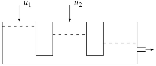
Figure 1. Three-tank system.

Clearly, model (27) is described by matrices, where $F=0$. To overcome this difficulty, we can transform (27) by introducing formal addends $-(x_1-x_2)+(x_1-x_2),$ $((x_1-x_2)-(x_2-x_3))-((x_1-x_2)-(x_2-x_3))$, and $(x_2-x_3-x_3)-(x_2-x_3-x_3)$ in the first, second, and third equations, respectively. Then $-(x_1-x_2)$ is added to the linear part and $(x_1-x_2)$ to the nonlinear part; other addends are considered analogously. As a result, the system is described by matrices and nonlinearities as follows:

$$\begin{array}{ccc}\hfill A& =& \left(\begin{array}{ccc}-1& 1& 0\\ 1& -2& 1\\ 0& 1& -2\end{array}\right),B=\left(\begin{array}{cc}1& 0\\ 0& 1\\ 0& 0\end{array}\right),C=\left(\begin{array}{ccc}0& 1& 0\\ 0& 0& 1\end{array}\right),D=\left(\begin{array}{c}0\\ 1\\ 0\end{array}\right),\hfill \\ \hfill G& =& \left(\begin{array}{ccc}1& 0& 0\\ -1& 1& 0\\ 0& -1& 1\end{array}\right),\Psi \left(x\right)=\left(\begin{array}{c}-\sqrt{P_{1}x}+P_{1}x\\ -\sqrt{P_{2}x}+P_{2}x\\ -\sqrt{P_{3}x}+P_{3}x\end{array}\right),\hfill \\ \hfill P_1& =& (1-10),P_2=(01-1),P_3=\left(001\right).\hfill \end{array}$$

Calculate interval estimates for $x\left(t\right).$

It follows from Section 4 that $x^{\left(1\right)}={(x_2,x_3)}^T,$ $x^{\left(2\right)}=x_1.$ Since $C_0=I_2$, we obtain

$$\begin{array}{ccc}\hfill {\underline{x}}_2\left(t\right)& =& y_1\left(t\right)-w_{*1}\left(t\right),{\overline{x}}_2\left(t\right)=y_1\left(t\right)+w_{*1}\left(t\right),\hfill \\ \hfill {\underline{x}}_3\left(t\right)& =& y_2\left(t\right)-w_{*2}\left(t\right),{\overline{x}}_3\left(t\right)=y_2\left(t\right)+w_{*2}\left(t\right).\hfill \end{array}$$

To estimate $z\left(t\right)=x_1\left(t\right)$, set $M:=\left(100\right)$, $D_0=\left(\begin{array}{ccc}1& 0& 0\\ 0& 0& 1\end{array}\right).$ Equation (7) becomes

$$(N_i-J_{*i})\left(\begin{array}{ccc}-1-\lambda & 1& 0\\ 0& 1& -2-\lambda \\ 0& 1& 0\\ 0& 0& 1\end{array}\right)=0.$$

Set $\lambda :=-1$ and obtain $k=1$ and $N=J_{*}=\left(10\right);$ as a result, $\Phi =\left(100\right),$ $B_{*}=\left(10\right),$ $D_{*}=0,$ $C_z=1$, $Q=0$, $G_{*}=\left(100\right).$ Clearly, the condition (25) is satisfied, and $P_{*1}=(1-10)$. Model (14) is of the form

$$\begin{array}{ccc}\hfill {\dot{x}}_{*}\left(t\right)& =& u_1\left(t\right)-\sqrt{x_{*}\left(t\right)-y_1\left(t\right)},\hfill \\ \hfill z\left(t\right)& =& x_{*}\left(t\right).\hfill \end{array}$$

Clearly, the model is stable; the function $“\sqrt{}”$ is monotonic. The interval observer estimating the variable $x_1\left(t\right)$ is given by

$$\begin{array}{ccc}\hfill {\dot{\underline{x}}}_1\left(t\right)& =& u_1\left(t\right)-\sqrt{{\underline{x}}_1\left(t\right)-y_1\left(t\right)}-k_{*}{w}_{*1}\left(t\right),\hfill \\ \hfill {\dot{\overline{x}}}_1\left(t\right)& =& u_1\left(t\right)-\sqrt{{\overline{x}}_1\left(t\right)-y_1\left(t\right)}+k_{*}{w}_{*1}\left(t\right).\hfill \end{array}$$

Note that the approach suggested in [2] gives the observer of dimension 6, and its estimates contain the disturbance $\rho \left(t\right)$, which is absent in our approach.

For the simulation, assume for simplicity that $a_1=a_2=\dots =a_6=1$, ${\vartheta }_7=0$; $\left|\rho \right|\le {\rho }_{*}$, $|w_1|\le w_{*1}$, $|w_2|\le w_{*2}$. Then take $u_1\left(t\right)=0.5$ and $u_2\left(t\right)=0.2$, $x_1\left(0\right)=3$, ${\underline{x}}_1\left(0\right)=1$, and ${\overline{x}}_1\left(0\right)=4$. The simulation results with $D\left[\rho \right]=0.6,$ $D\left[w_1\right]=0.1,$ $k_{*}{w}_{*1}=0.3$ and $\rho =0,$ $D\left[w_1\right]=0.2,$ $k_{*}{w}_{*1}=0.6$ are shown in Figure 2 and Figure 3, respectively, where the graphs of the functions $x_1\left(t\right)$, ${\underline{x}}_1\left(t\right)$, and ${\overline{x}}_1\left(t\right)$ are presented. Clearly, the product $k_{*}{w}_{*1}$ is greater, and the interval ${\underline{x}}_1\left(t\right),{\overline{x}}_1\left(t\right)$ is wider. Moreover, the value of the disturbance $\rho$ does not affect the interval width; this confirms that the model is decoupled from the disturbance.

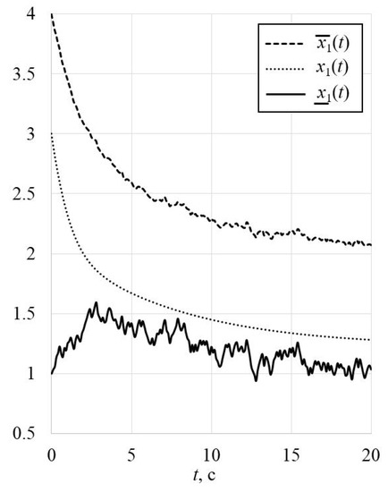
Figure 2. Graphs of the functions $x_1\left(t\right)$, ${\underline{x}}_1\left(t\right)$, and ${\overline{x}}_1\left(t\right)$ with $k_{*}{w}_{*1}=0.3$ and $D\left[\rho \right]=0.6$.

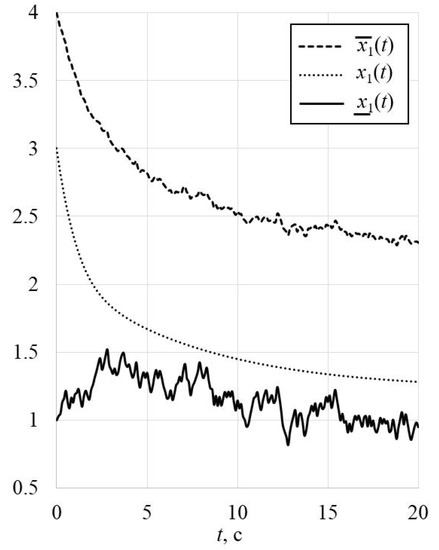
Figure 3. Graphs of the functions $x_1\left(t\right)$, ${\underline{x}}_1\left(t\right)$, and ${\overline{x}}_1\left(t\right)$ with $k_{*}{w}_{*1}=0.6$ and $\rho =0$.

9. Discussion

The problems of designing diagnostic observers, virtual sensors, interval observers, and sliding mode observers based on the Jordan canonical form have been addressed and resolved. The methods for solving these problems have been developed for both linear and nonlinear systems, taking into account external disturbances and measurement noise. The observers are based on the reduced-order model of the original system; they are invariant with respect to the disturbance or have minimal sensitivity to the disturbance. It was shown that when the invariance, with respect to the disturbance, can be achieved, the JCF allows reducing the dimensions of observers and virtual sensors, making the design procedure simpler when compared with the ICF. On the other hand, when the invariance, with respect to the disturbance, is impossible, and a robust solution is used, the JCF has to use more complex rules to minimize the impact of the disturbance in the model. Moreover, the JCF restricts the possibility of this minimization. An analysis has shown that, in this case, ICF is preferable; it enables minimizing the contribution of the disturbance more effectively. This is not true for the interval observer since the transformation of the ICF model, designed on the basis of the singular value decomposition into the JCF model, may increase the contribution of the disturbance. Theoretical results are illustrated through the well-known tree-tank system. Future work will investigate the JCF stability in the system with external disturbance.

References

- Blanke, M.; Kinnaert, M.; Lunze, J.; Staroswiecki, M. Diagnosis and Fault-Tolerant Control; Springer: Berlin, Germany, 2016. [Google Scholar]
- Efimov, D.; Raissi, T. Design of interval state observers for uncertain dynamical systems. Autom. Remote Control 2016, 77, 191–225. [Google Scholar] [CrossRef]
- Kwakernaak, H.; Sivan, R. Linear Optimal Control Systems; Wiley-Interscience: London, UK, 1972. [Google Scholar]
- Misawa, E.; Hedrick, J. Nonlinear observers—A state of the art survey. J. Dyn. Syst. Meas. Control 1989, 111, 344–352. [Google Scholar] [CrossRef]
- Zhirabok, A.; Shumsky, A.; Pavlov, S. Diagnosis of linear dynamic systems by the nonparametric method. Autom. Remote Control 2017, 78, 1173–1188. [Google Scholar] [CrossRef]
- Efimov, D.; Polyakov, A.; Richard, J. Interval observer design for estimation and control of time-delay descriptor systems. Eur. J. Control 2015, 23, 26–35. [Google Scholar] [CrossRef]
- Khan, A.; Xie, W.; Zhang, L.; Liu, L. Design and applications of interval observers for uncertain dynamical systems. IET Circuits Devices Syst. 2020, 14, 721–740. [Google Scholar] [CrossRef]
- Kolesov, N.V.; Gruzlikov, A.M.; Lukoyanov, E.V. Using fuzzy interacting observers for fault diagnosis in systems with parametric uncertainty. Procedia Comput. Sci. 2017, 103, 499–504. [Google Scholar]
- Mazenc, F.; Dinh, T.; Niculescu, S. Interval observers for discrete-time systems. Inter. J. Robust Nonlinear Control 2014, 24, 2867–2890. [Google Scholar] [CrossRef]
- Raissi, T.; Efimov, D.; Zolghadri, A. Interval state estimation for a class of nonlinear systems. IEEE Trans. Autom. Control 2012, 57, 260–265. [Google Scholar] [CrossRef]
- Rotondo, D.; Fernanez-Canti, R.; Tornil-Sin, S. Robust fault diagnosis of proton exchange membrane fuel cells using a Takagi-Sugeno interval observer approach. Int. J. Hydrogen Energy 2016, 41, 2875–2886. [Google Scholar] [CrossRef]
- Zhang, K.; Jiang, B.; Yan, X.; Edwards, C. Interval sliding mode based fault accommodation for non-minimal phase LPV systems with online control application. Intern. J. Control 2019, 93, 2675–2689. [Google Scholar] [CrossRef]
- Zhirabok, A. Error selfcorrection in discrete dynamic systems. Autom. Remote Control 2006, 67, 868–879. [Google Scholar] [CrossRef]
- Witczak, M. Fault Diagnosis and Fault Tolerant Control Strategies for Nonlinear Systems; Springer: Berlin, Germany, 2014. [Google Scholar]
- Zhirabok, A.; Shumsky, A.; Solyanik, S.; Suvorov, A. Fault detection in nonlinear systems via linear methods. Int. J. Appl. Math. Comput. Sci. 2017, 27, 261–272. [Google Scholar] [CrossRef]
- Blesa, J.; Rotondo, D.; Puig, V. FDI and FTC of wind turbines using the interval observer approach and virtual actuators/sensors. Control Eng. Pract. 2014, 24, 138–155. [Google Scholar] [CrossRef]
- Jove, E.; Casteleiro-Roca, J.; Quntian, H.; Mendez-Perez, J.; Calvo-Rolle, J. Virtual sensor for fault detection, isolation and data recovery for bicomponent mixing machine monitoring. Informatica 2019, 30, 671–687. [Google Scholar] [CrossRef]
- Hosseinpoor, Z.; Arefi, M.; Razavi-Far, R.; Mozafari, N.; Hazbavi, S. Virtual sensors for fault diagnosis: A case of induction motor broken rotor bar. IEEE Sens. J. 2021, 21, 5044–5051. [Google Scholar] [CrossRef]
- Zhirabok, A.; Kim, C. Virtual sensors for the functional diagnosis of nonlinear systems. J. Comput. Syst. Sci. Int. 2022, 61, 67–75. [Google Scholar] [CrossRef]
- Degue, K.; Efimov, D.; Richard, J. Interval observers for linear impulsive systems. IFAC-PapersOnLine 2016, 49, 867–872. [Google Scholar] [CrossRef]
- Dinh, N.; Mazenc, F.; Niculescu, S. Interval observer composed of observers for nonlinear systems. In Proceedings of the 2014 European Control Conference (ECC), Strasbourg, France, 24–27 June 2014; pp. 660–665. [Google Scholar]
- Mazenc, F.; Bernard, O. Interval observers for linear time-invariant systems with disturbances. Automatica 2011, 47, 140–147. [Google Scholar] [CrossRef]
- Efimov, D.; Perruquetti, W.; Raissi, T.; Zolghadri, A. Interval observers for time-varying discrete-time systems. IEEE Trans. Autom. Control 2013, 58, 3218–3224. [Google Scholar] [CrossRef]
- Sergiyenko, O.; Zhirabok, A.; Ibraheem, I.; Zuev, A.; Filaretov, V.; Azar, A.; Hameed, I. Interval observers for discrete-time linear systems with uncertainties. Symmetry 2022, 14, 2131. [Google Scholar] [CrossRef]
- Chang, J.; Tan, C.; Trinh, H.; Kamal, M. State and fault estimation for a class of non-infinitely observable descriptor systems using two sliding mode observers in cascade. J. Frankl. Inst. 2019, 356, 3010–3029. [Google Scholar] [CrossRef]
- Edwards, C.; Spurgeon, S.; Patton, R. Sliding mode observers for fault detection and isolation. Automatica 2000, 36, 541–553. [Google Scholar] [CrossRef]
- Fridman, L.; Levant, A.; Davila, J. Observation of linear systems with unknown inputs via high-order sliding-modes. Int. J. Syst. Sci. 2007, 38, 773–791. [Google Scholar] [CrossRef]
- Sergiyenko, O.; Tyrsa, V.; Zhirabok, A.; Zuev, A. Sensor fault identification in linear and nonlinear dynamic systems via sliding mode observers. IEEE Sens. J. 2022, 22, 10173–10182. [Google Scholar] [CrossRef]
- Shtessel, Y.; Edwards, C.; Fridman, L.; Levant, A. Sliding Mode Control and Observation; Springer: Berlin, Germany, 2014. [Google Scholar]
- Wang, X.; Tan, C.; Zhou, D. A novel sliding mode observer for state and fault estimation in systems not satisfing maching and minimum phase conditions. Automatica 2017, 79, 290–295. [Google Scholar] [CrossRef]
- Yan, X.; Edwards, C. Nonlinear robust fault reconstruction and estimation using a sliding modes observer. Automatica 2007, 43, 1605–1614. [Google Scholar] [CrossRef]
- Zhirabok, A.; Shumsky, A.; Zuev, A. Fault diagnosis in linear systems via sliding mode observers. Int. J. Control 2021, 94, 327–335. [Google Scholar] [CrossRef]
- Zhirabok, A.; Zuev, A.; Seriyenko, O.; Shumsky, A. Fault identificaition in nonlinear dynamic systems and their sensors based on sliding mode observers. Autom. Remote Control 2022, 83, 214–236. [Google Scholar] [CrossRef]
- Castillo, I.; Fridman, L.; Moreno, J. Super-twisting algorithm in presence of time and state dependent perturbations. Int. J. Control 2018, 91, 2535–2548. [Google Scholar] [CrossRef]
- Tan, C.; Edwards, C. Sliding mode observers for robust detection and reconstruction of actuator and sensor faults. Int. J. Robust Nonlinear Control 2003, 13, 443–463. [Google Scholar] [CrossRef]
- Zhirabok, A.; Zuev, A.; Filaretov, V.; Shumsky, A. Sliding mode observers for fault identification in linear systems not satisfying matching and minimum phase conditions. Arch. Control Sci. 2021, 31, 253–266. [Google Scholar]
- Low, X.; Willsky, A.; Verghese, G. Optimally robust redundancy relations for failure detection in uncertain systems. Automatica 1996, 22, 333–344. [Google Scholar]
Disclaimer/Publisher’s Note: The statements, opinions and data contained in all publications are solely those of the individual author(s) and contributor(s) and not of MDPI and/or the editor(s). MDPI and/or the editor(s) disclaim responsibility for any injury to people or property resulting from any ideas, methods, instructions or products referred to in the content. |
© 2023 by the authors. Licensee MDPI, Basel, Switzerland. This article is an open access article distributed under the terms and conditions of the Creative Commons Attribution (CC BY) license (https://creativecommons.org/licenses/by/4.0/).