Abstract
Higher dimensionality, Hughes phenomenon, spatial resolution of image data, and presence of mixed pixels are the main challenges in a multi-spectral image classification process. Most of the classical machine learning algorithms suffer from scoring optimal classification performance over multi-spectral image data. In this study, we propose stack-based ensemble-based learning approach to optimize image classification performance. In addition, we integrate the proposed ensemble learning with XGBoost method to further improve its classification accuracy. To conduct the experiment, the Landsat image data has been acquired from Bishoftu town located in the Oromia region of Ethiopia. The current study’s main objective was to assess the performance of land cover and land use analysis using multi-spectral image data. Results from our experiment indicate that, the proposed ensemble learning method outperforms any strong base classifiers with 99.96% classification performance accuracy.
1. Introduction
Ethiopia is the second most populous country after Nigeria on the African continent. According to United Nation reports, more than 85% of the population is primarily dependent on agriculture for their economic activity and livelihood [1,2].The agriculture sector is still based on subsistence farming using traditional methods such as ox-drawn ploughs with very little mechanization [3,4]. For thousands of years, agriculture in Ethiopia has been practiced using traditional methods and tools. In addition, due to recurrent droughts, the country was unable to feed a portion of its burgeoning population [5], now estimated at 110 million. The other limitation in the agricultural sector was lack of a decision support system for the purposes of land-cover analysis, disease monitoring system, yield prediction mechanism, and efficient weather monitoring methods.
On the other hand, the current state-of-the-art in the agricultural domain requires an application of high-tech to improve production and productivity. In this regard, Mahmoud A. and colleague [6] proposed Precision agriculture is an approach to use information technology to improve the quality of crops and increase yields. Precision Agriculture has been defined as maximizing yields using minimal resources such as water, fertilizer, pesticides and seeds by Spyridon, N. and his colleague [7]. Similarly, Alaa, A. and his colleague [8] well defined the concepts of Precision agriculture as a farm management system using information technology to identify, analyze and manage the variability of fields to ensure profitability, sustainability, and protection of the environment. In addition, computer vision (CV) [9,10,11] and machine learning models play a significant roles to determine soil properties. According to Kariheinz Knickel [3], since the 1950s and 1960s, agricultural modernization vigorously entrenched and established a form of agriculture that is capital-intensive, high-input, high-output, specialized and rationalized system by industrial countries. To achieve sustainable agricultural output [8], precision agriculture is used and it is the technology that can enhance the farming process. Recently, AI and machine learning simplified the complex process of data collection, data processing, data-interpretation and decision-making strategy in the agriculture sector. Similarly, the advancement of remote sensing technologies [12] significantly shifted the trends of agricultural practices. Quite larger numbers of studies have been reported that, remote sensing technologies are predominantly utilized to enhance production quality and crop health monitoring purposes.
Due to the rich information contained, in them, in this study, our dataset includes multi-spectral images. The research community in the domain area classified remote sensing data into multi-spectral and hyper-spectral image data. The only difference between the two data types are the ranges of numbers of bands employed to solve the problem at hand. Knickel and his colleague [3], defined remote sensing as a method of extracting or acquiring relevant information about earth’s surface [13] by analyzing the extracted hyperspectral features. Hyperspectral image data comprises multiple bands [4,12,14] that are sensitive to a very narrow wavelength range along the electromagnetic spectrum [12,15]. Hyperspectral imaging is preferred because of its cost-effectiveness [16], the non-destructive measurement of biophysical and biochemical properties of object on the surface, and the ease to analyzing image data in real-time. The advantage is even more pronounced when one considers the fact that processing handcrafted image data is time a consuming endeavor and getting high quality images is very expensive.
In this study, we propose and test an ensemble-based machine learning approach to classify remotely sensed image data collected from around Bishoftu, located in the Oromia Region of Ethiopia. The area is rich in terms of its bio-diversity and large portions of the land are covered with cereal crops. In the work, our main objective was to utilize multi-spectral image to analyze land-cover [10] and land-use. Application of multi-spectral image data in the agriculture domain allows us to make valuable contributions by addressing the challenges of traditional data collection, interpretation, and analysis. In addition, such system reduce the time and effort of domain experts to process large-sized image data quickly and efficiently.
The proposed stack-based ensemble learning approach will have the following contributions to the multi-spectral image process for land-use land-cover analysis:
- Crafting automatic spatial-spectral feature extraction, in order to resolve the challenges of manual region of interest (ROI) due to labeling.
- Optimizing the classification performance of the proposed ensemble-based machine learning model. Most GIS tools have a built-in classical machine learning model to classify land-use and land-cover. But, due to the complex nature of multi-spectral image data, these models suffer from a few limitations and fail to get optimal classification performance.
- Our target was to design an ensemble learning approach to address the challenges of bias-variance trade-off, which is the limitation of many classical machine learning models. Many classical models are sensitive, small changes in the training data will brought a significant change on the performance of the classifiers.
2. Review of Related Works
A self-trained ensemble with semi-supervised support vector machine for pixel classification of remote sensing imagery had been proposed by Maulik and Chakraborty [17]. He ensemble was based on application of the margin maximization principle to both labeled and unlabeled data. In the semi-supervised support vector machine (SS-SVM) approach, the classifier uses majority voting [18] to classify a pixel into its respective category.Maulik and Chakraborty recommend that the Mahalanobis distance can be utilized to query the correlated points from the unlabeled database when designing the various self-trained methods. The Mahalanobis distance is an effective multivariate distance metric that measures the distance between a point and the mean value of a distribution. It is an extremely useful distance metric with applications in multivariate anomaly detection, classification on highly imbalanced datasets, and one-class classification. Another useful approach is the rotation-based SVM (RoSVM) ensemble in the classification of hyperspectral data with limited training samples. The basic idea of RoSVM is to generate diverse SVM classification results using random feature selection and data transformation. This approach can enhance both individual accuracy and diversity within the ensemble (PCA and projection). Its main weakness is the higher than normal computational complexity; compared to SVM and RSSVM [19]. A fast learning method recommended by the authors, a combination of SVMs and multiple classifier system (MCS) for the classification of hyperspectral data and a semi-supervised approach, is another effective method to deal with limited training samples and RoSVM’s drawback. Similarly, Fang and his colleague [18] proposed the Adaptive Rotation forest (RoF) model to handle the challenge of class-imbalance due to limited training sample. Fei LV [20] inspired extreme learning machine with auto-encoder to solve ineffective classification of data due to inadequate labeled training.
2.1. High Dimensional Hyperspectral Image Data
Hyperspectral image data contains hundreds of data channels with a large and various number of features. Consequently, dimensional issues are the striking challenge when it comes to processing such multi-spectral images. Similarly, down-sizing the numbers of dimensions will also cause the processing to eliminate some relevant features from the image data. The dimensionality challenge [21,22] creates the Hughes phenomenon, a well-known problem in the classification domain where an initial increase in the number of features leads to an increase in a classifier’s performance load until an optimal number of features is reached. Most conventional machine learning models fail to handle this phenomenon well and lead to poor performance. Ceamanos and his colleagues [23] inspired the fusion approach to handle high dimensionality. The authors decomposed a large image dataset into sub-samples [24,25] and trained each by using the standard SVM model. The prediction output from each model was then fused using another SVM. Similarly, Mohamed [26] combined the SVM model with a bagging technique to handle the n-dimensional hyperspectral dataset. The study attempted to minimize prediction variances and, thus, improve overall accuracy. On the other hand, Xia and his colleague [27] proposed a novel ensemble based canonical correlation forest to address challenges associated with high-dimensionality. The authors employed principal component analysis (PCA) on each subset to transform the input data into a new feature space. Then, the final classification results were determined by the prediction of individual canonical correlation trees (CCTs ) using a majority voting rule. However, it is not clear why [27] used the majority voting rule to produce the final classification result. On the other hand, it is clear that the curse of dimensionality degraded classification accuracy. To tackle this challenge, Juang, Ch. X. and his colleagues [28] proposed the fuzzy C-means based support vector machine or SVM-fuzzy C-mean. The SVM was used for band selection purposes whereas the C-mean method was used to build an ensemble of clustering maps. The Markov fisher selector has been used to minimize computation complexity during the clustering process. They utilized majority voting technique and Markov random field theory to fuse the final model. Similarly, Samat and colleagues [29] also proposed an ensemble extreme learning method to resolve high-dimensionality problems. Bagging-based and adaptive boost (AdaBoosting) based ensemble schemes have been used to conduct experiment on the Reflective Optics System Imaging Spectrometer (ROSIS) and the Airborne Visible Infrared Imaging Spectrometer (AVIRIS) [30] data. According to the authors, a differential and non-differential parameters with a kernel based activation function can be used to improve classification performance of the proposed model. Therefore, handling the dimensionality issues will significantly improve the classification performance.
2.2. Feature Extraction
Other challenges in multi-spectral image processing were extracting features used to train a machine learning model. Manual feature extraction techniques are resource-intensive and time- consuming processes compared to other state-of-the-art methodologies. To tackle the limitation, a lot of attempts have been made in the domain area. Merentitis and his colleague utilized principal component analysis [15] to handle dimension reduction issues and Feature Extraction (FE) techniques for massive datasets. Some authors argue that these techniques have a limitation: they ignore correlation between neighboring features or pixels. Similarly, Parshakov and his colleague [31] inspired a Spectral Angel Mapper technique to map a cluster of pixel values instead of individual pixels. A unified framework method has also been inspired by Merentitis [32] to address bias-variance decomposition. Merentitis, introduced MNF transformation, blind unmixing and derivation of abundance maps (Ams), non-parametric weighted feature extraction (NWFE), and synthetic features methods to resolve the trade-off. On the other hand, Zhong and Liu [19] proposed a binary classifier or dichotomizer technique to separate subsets of classes. Another important concern in multi-spectral images is the issue of combining spectral and spatial features. To resolve the challenge, Chen and his colleague employ a Gabor-filtering and kernel based extreme learning machine (KELM) classifier and multi-hypothesis (MH)-prediction-based approach and they proposed and applied the approach to produce superior results compared to pixel-wise classification. Similarly, Ergul and Bilgin [33] combined spatial circle-neighborhood information with a semi-supervised classifier approach [34] to extract relevant features from image data. Random Multi-Graphs (RMGs) for spectral and spatial classification framework and matrix-based spatial-spectral feature representation have been used by Hang et al. [34] Likewise, Shaohui Mei and his colleague proposed the CNN method to extract relevant features to train a deep stacked neural network (DSNN) model. Shaohui applied a fusion approach to concatenate the extracted features. Pan and colleague [35] also proposed Hierarchical guidance filtering based ensemble learning to integrate the spatial and spectral feature from HSI data. In addition, an Adaptive Boosting (AdaBoost) approach has been used by Chenming Qi and his colleague [36] to minimize redundancy and maximize relevance in feature extraction process. The authors argue that, a mutual information based ensemble learning classifier outperforms similar classifiers for multi-class classification problems. There are hundreds of feature extraction techniques available. Machine learning researchers and experts are expected to critically assess the appropriate feature extraction approaches to tackle the challenges of model over-fitting.
A good generalizable machine learning models mainly depends on the wealth of the training dataset. In this regard, on the size of the training dataset causes the model either to under-fit or over-fit on the testing or validation data. Preparing adequate representative datasets is an important consideration when designing machine learning models. The research community in the domain area attempted to handle the limitation of small-size training datasets in multi-spectral image processing. Li and his colleagues [37], argue that classification performance suffers due to training model having limited labeled training samples [19]. In case of multi-spectral image classification, training samples need to be considered carefully to reduce model over-fitting. According to Maulik, Ujjwal [17], one of the possible solutions to limited training samples was applying the semi-supervised approach to classify multi-spectral image data. In semi-supervised approach, one combine [38] limited labeled samples [39] with large unlabeled samples to exploit the abundance of unlabeled samples. Similarly, Ramzi and his colleague [40] highlighted that, for a broad range of spectral bands, it is often difficult to find sufficient number of training samples. In addition, Fang and colleague [18] proposed a multi-Scale CNN to extract features from an unlabeled data. The multi-scale classifier is used to assign a label to unlabeled sample. A majority voting schema have been used to select an unlabeled image with a predefined threshold. Finally, the selected sample instances are added to the original training data to be used in subsequent training iterations. In addition, image quality is a big concern in the area of multi-spectral image classification. To tackle this pitfall, the research community proposed different approaches such as denoising [25,41,42] feature reconstruction, super-resolution methodologies and image recovering technique. On the other hand, Xia and his colleague [43] the proposed Random Forest ensemble where extended multi-extinction profiles are implemented to improve classification performance. They used different boosting strategies to construct the ensemble model.
Therefore, from the review of related works, it is apparent that very optimal classification performance is difficult to achieve without having adequate training samples. In the current study, our main objective was to mitigate the challenges of models bias-variance and enhancing classification performance. The proposed stack-based ensemble learning model performs well to handle the complex multi-spectral image data.
3. Stack-Based Ensemble Learning Model
Stacking is an ensemble learning technique to combine multiple base classification models via a meta-classifier. This approach combines multiple conventional classifiers to build one generalized machine learning model. First different base learning models are trained on the same dataset which consists of examples i.e., pairs of feature vectors () and its corresponding target class . To generate a training set for learning the meta-level classifier, a leave-one-out or a cross validation procedure is applied. The proposed stacked-based ensemble learning model has been presented on Figure 1 below.
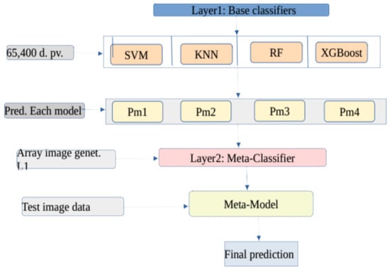
Figure 1.
Proposed model architecture.
Note: d.pv represent input dimensional pixel values, and constructed a new L1 represents array of image data generated from each first level classifiers and pm1 to pm4 represents the prediction output of first level classifier respectively.
The improved version of the stacking algorithm is presented in Figure 2 below and it can be summarized as follows: From the raster image data about 65,000 features are used as input dimension vectors to train first level classifier. First, we trained h first level classifiers with D input dimension. In the current study, we have utilized four first level classifiers to fit the training data. From the prediction output of each first level classifier, we generated a new training data-set . The meta-classifier was trained using to fit the stacking model: . To mitigate the over-fitting challenge, we applied cross-validation techniques to split the training data into 10 fold. Let implies be an index function that indicates the partition to which observation i is allocated by the randomization.
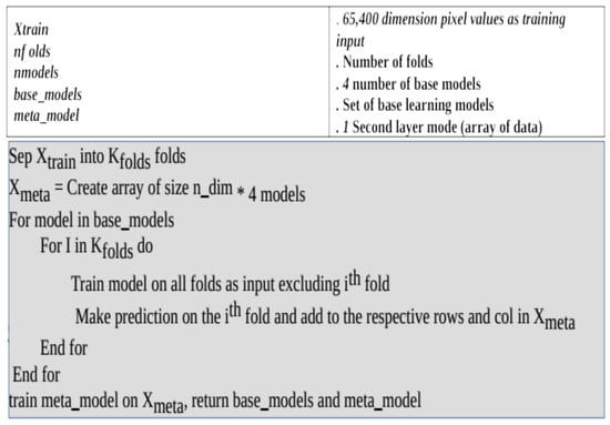
Figure 2.
Stacked based ensemble learning algorithm.
4. Experiment Results and Discussion
Datasets
To conduct the experiment, LandSat image data has been collected from Yerer Selassie located near the town of Bishoftu in the Oromia region of Ethiopia. Yerer is located in the East Shewa zone in the great rift valley at 38°57′40.863″ E and 8°50′55.016″ N. Yerer selassie borders on the south by Dugda Bora to the south the West Shewa Zone to the West, the town of Akaki to the Northwest, the district of Gimbichu to the northeast, and of Lome to the east. Altitudes in this district range from 1500 to over 2000 m above sea level. From this specific geo-location, three image data were collected in different time frames.
During the data pre-processing steps, we made all the required corrections such as: determining Spatial resolution using operational land imagery, Top of Atmosphere Reflectance, Radiometric correction and Topographic Correction, and Generating False color composition . About four bands namely the red, blue, green and near-Infrared bands have been selected to extract the relevant features. Layer stacking has been performed to combine all four selected spectral bands to obtain a single stacked image data. At this level, one can utilize different false color combinations to make the visualization of the stacked image appear more natural. Figure 3 shows the image stacking process we utilized.
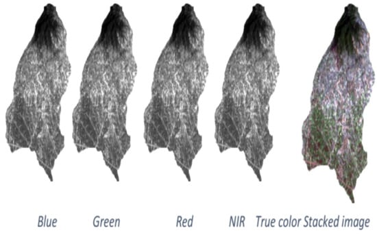
Figure 3.
Stacking the bands together.
The stacked multi-spectral image was used as an input dataset to train the proposed model which comprises a dimension of 372 nrow ∗ 200 ncol, 30 m spatial resolution, and a total of 65,400 features. A sample or observation of 147 spatial-polygon has been labeled as a training dataset from the raster image data. The distribution provides a parameterized mathematical function that can be used to calculate the probability for any individual observation from the sample space. From this analogy, the training datasets are almost evenly distributed. Figure 4 illustrates the distribution of training samples on each layer stack.
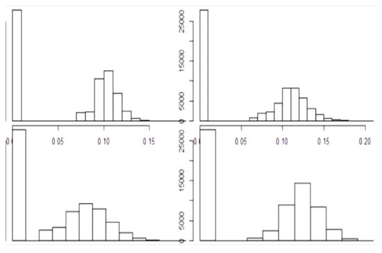
Figure 4.
The Statistical distribution of training data-set.
Then, the dataset split and 70% of it was used for training purposes and the remaining 30% was used for model testing purpose. The next step was applying multiple base classifiers to build our classification models. In this regard, we selected models as base classifiers. All the base classifiers utilized , , nd the bootstrapped sampling technique was used to select sample dataset. The Samples were constructed by drawing observations from a large data sample one at a time and returning them to the data sample after they have been chosen. This allows a given observation to be included in a given small sample more than once. In this sub-section, we briefly discuss the nature of the individual base classifiers. First, the support vector machine is one of the strong machine learning algorithms provided non-linear issues are properly handled. We have utilized the RBF kernel function to fit the model. The radial kernel function has a form:
where is a tuning parameter which accounts for the smoothness of the decision boundary and controls the variance of the model. If is very large then we get quiet fluctuating and wiggly decision boundaries which accounts for high variance and over-fitting. If is small, the decision line or boundary is smoother and has low variance. Then the support of SVM becomes:
The second base classifier is the random forest (RF) classifier which is an ensemble learner by its very nature. It a classifier comprising a number of decision trees on various subsets of the given observation and takes the average to improve the predictive accuracy of that dataset. The output chosen by the majority of the decision trees becomes the final output of the rain forest system. The third base classifier was the KNN algorithm that stores all the available data and classifies a new data point based on similarity. That is, when new data appears, then it can be easily classified into a category by using the KNN algorithm. KNN is a non-parametric algorithm, which means it does not make any assumptions about the underlying data. There is no particular way to determine the best value for “K”, so we need to try some values to find the best performing one. The most preferred value for K is 5.
where, x and y are the two vector points on sample space. Optimal classification performance obtained at .
Table 1 above summarizes experiment results and the classification performance of each base classifier on the training data-sets. Generally, each classifiers performs very well on the training data. In the case of KNN, the new training samples were classified into their respective categories by a majority vote of its neighbors, with the case being assigned to the class most common amongst its K nearest neighbors measured by a distance function. There is no standard to define the numbers of K values. It needs several trial and errors to get the optimal values. On the other hand, we have evaluate different distance metrics that fit the problem domain. Similarly, SVM needs to address the non-linearity issue by finding the best fitting kernel function. The idea behind generating non-linear decision boundaries is that we need to do some nonlinear transformations on the features , which transforms them into a higher dimensional space. In our case, the non-linear decision boundary and the values of the tuning parameters were and a number of support vectors. Results of the experiment show that the number of predictors affects the classification performance of each base classifier. In this regard, as the number of predictors increases or decreases, the performance of the model also varies. The last but not least base classifier was the XGBoost method [37,38,39]. Assume that our image dataset is D = (, ): i = 1 … n, ɛ , ɛ , then we get n observations with m dimensions each and with a target class y. Let ŷi be defined as a result given by the ensemble represented by the generalized model as follows [43]:
where is a regression tree, and represents the score given by the k-th tree to the i-th observation in the data. In order to define function , the following regularized objective function should be minimized:
L is the loss function. In order to prevent the model from getting too large and complex, the penalty term is included as follows:
where Y and are parameters controlling penalty for the number of leaves T and the magnitude of leaf weights w, respectively. The purpose of is to prevent over-fitting while simplifying models produced by this algorithm.

Table 1.
Summary of base classifiers accuracy on the training datasets.
Note: The final values used for the model were , , , , , .
After evaluating the performance of individual base classifier, we employed the remaining 30% of our test data-set to evaluate the overall prediction performance of each base classifier. Table 2 summarizes the prediction performance of the base classifiers using the test dataset.
Table 2.
Summary of the four model prediction accuracy.
From Table 2, one can deduce that all the models performed well in classifying the test dataset with high accuracy. However, when we compared the prediction performance of KNN and SVM on test and training data-sets, we encountered an issue an issue over-fitting. One of the possible solutions is increasing the sizes of both the training and testing data set. Another challenge is, the sensitive of base classifiers, where small variances significantly affected their prediction performance. The main objective of this study was to implement stack-based ensemble learning method. In ensemble learning method, before proceeding to combine different base classifier, evaluating the correlation among individual base classifiers are very import. If there is no difference among base classifier, then no need of applying Ensembling learning approach. The rules of ensemble-based learning are mainly based on difference among base classifiers. From our experimental results, the correlation among the base classifiers are briefly summarized in Table 3.
Table 3.
Correlation among selected base classifier models.
In Table 3, the pairwise correlations between individual models are low and fulfill the requirement of an ensemble learning rule. From experiment results, two models are highly correlated in predicting the training data-sets. Building the ensemble learning demand the analogy of less difference among the base classifiers. Due to the bootstrap re-sampling, the size of selected samples in each target classes are differ at different executions. The base classifier sensitivity was also observed in the correlation among the models.
Once the assessment has been completed, the next step was implementing the stack-based ensemble learning approach to determine the final categories using meta-data. The stacking approach utilizes meta-data generated from each base classifier as input for training the meta-model. Bagging namely bootstrap aggregating [44,45] is one of the most intuitive and simple frameworks in ensemble learning that uses the bootstrapped sampling method. In this method, many original training samples may be repeated in the resulting training data, whereas others may be left out. Samples are selected randomly from the training set, instructive iteration is applied to create different bags, and the weak learner is trained in each bag. Each base learner predicts the label of the unknown sample, respectively.
In the case of Stacked XGBoosting method, a multi-nominal distribution sampling technique has been used to select observations randomly from the sample space. First, the parameters are sorted in descending order. Then, for each trial, variable X is drawn from a uniform distribution. The resulting outcome is the component.
= 1; = 0 for is one observation from the multi-nomial distribution with and . A sum of independent repetitions of this experiment is an observation from a multi-nominal distribution with n equal to the number of such repetitions. Our overall results from the experiment, in terms of the classification accuracy of the base and ensemble models are summarized in Table 4.
Table 4.
Overall accuracy of the base and ensemble classifier.
It is apparent from Table 4 that the majority of the individual base classifiers have classified both the training and testing datasets with satisfactory accuracies. When the base classifiers were combined using the stacking ensemble approach, the performance improved. The proposed model classified the multi-spectral image data with 99.96% classification accuracy. This is promising and the model is worth applying for various application areas. We plan to extend our work to further test the proposed model using larger image datasets. In this study, handling the challenges of bias and variance is our concern. To resolve this pitfall, we integrate the XGBoosting method into the ensemble learning approach. The XGBoost model belongs to a family of boosting algorithms that turn weak learners into strong learners. Boosting is a sequential process; i.e., trees are grown using the information from a previous grown tree one after the other. This process slowly learns from previously use of data and tries to improve its prediction in subsequent iterations. Boosting reduces
Both variance and bias. It reduces variance because it uses multiple models through a bagging process. It also reduces bias through training successive models by passing information on errors made by previous models. These are some of the reasons why we integrated the XGBoosting method into the stacking learning approach to address the challenges of bias-variance trade-off. In addition, Samat and colleague [25] also proposed the Meta-XGBoosting framework to improve the limitations of the XGBoost model. Finally, the XGBoost model enabled us to achieve optimal classification accuracy from the proposed model.
5. Discussion
Currently, remote sense image processing plays significant roles in the domain of agriculture. One of the broader application areas was to conduct land use and land cover (LULC) analysis using multi-spectral image data. A proper land cover management provides insights into how to efficiently utilize scarce natural resources. In addition, this is one of the ways forwarded for designing a mechanism to implement precision agriculture approaches in the sector. Table 5 provides an example data collected on the land cover of our study area.
Table 5.
The pattern of Land-cover from September to November.
From Table 5, the land-cover dynamically becomes bare land within 1.5 months. This is due the fact that the majority of the crops are harvested during this period. Table 5 also shows the patterns of land-use and land-cover by different classes over three months. Based on the insight obtained from the pattern, one could draw an informed decision.
In addition, we assessed the importance of variables (spectral bands) importance to examine which bands are important to classify the land-cover. To classify the land-cover, we used the blue, green, red and near-Infrared spectrum. These visible wavelengths cover a range from approximately 400 to 700 nano meter. Each spectrum characterizes objects on the surface by unique spectral signature. Blue spectrum is widely responsible for increasing plant quality specifically crop leaf. Similarly, the green spectrum absorb and used for photosynthesis. On the other hand, the red wavelength helps stem, leaf and general vegetation growth. Table 6 shows variable importance in ranked order from the highest to the lowest during model fitting using training data.
Table 6.
Variable importance assessment.
Variable importance assessment gives insight about the relevance of each bands used to build the first level classifiers. From the experimental result, Band 2 and Band 3 are the most important variables used to classify the training data-sets into the respective categories. To deal with multi-spectral image data, good understanding about the nature of data would help to handle the complexity.
Machine learning are a cost effective and efficient approach to analyze land-cover and land-use in the domain of multi-spectral image processing.Those tools have built-in image classifiers to label and classify the target classes. Figure 5 below present the semi-automated multi-spectral image data training data labeling process.
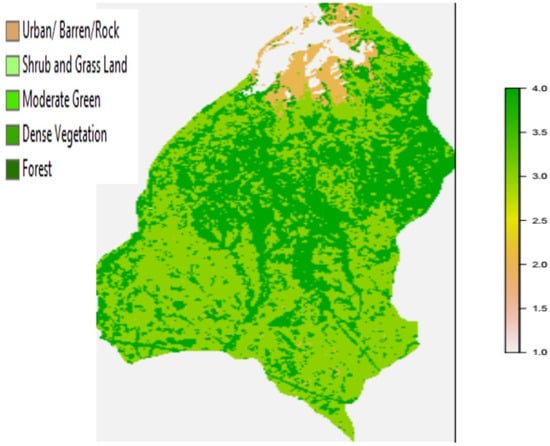
Figure 5.
XGBoost model classification output.
Manually training data-set labeling using a polygon (region of interest) methods were prone to biases and error due to mixed pixel values. Similarly, most of conventional machine learning models fail to handle the complexity of multi-spectral image data due to their higher dimensionality, the Hughes phenomenon resulting from unbalanced training samples, poor spatial and spectral resolution of the image data, large size of spectral features, and presence of mixed pixels. The process of semi-automatic feature extraction has been plotted on Figure 6 below.

Figure 6.
Semi-Automatic feature extraction using ErdaImagine.
In case of multi-spectral image classification, data preprocessing and correction are the bed-rock to obtain robust classification accuracy. Extracting relevant feature from multi-spectral image data to label the target class is a tricky task. In this study, we extracted a feature from each bands namely red, green, blue, near infrared bands to represent each pixel values. The stacked image was the combination of the above four band to represent classes of land cover in our study area. We have used R programming language scripts to automatically extract pixel values from the image data.
We have also used the Random Forest, Support Vector Machine, K-Nearest Neighbor, and XGBoost as base classifiers. With well labeled training datasets, the classifiers were competent enough to classify the test dataset into its respective categories. Generally, the issues of bias and variances are the big concern to be addressed by the proposed model.
Therefore, the proposed stack-based ensemble model using the XGBoosting method has been used to classify multi-spectral image data. An ensemble learning approach integrated with the extreme gradient boosting (XGBoost) method handled the bias and variance challenges of base classifiers much better. Based on experimental results, our proposed stack-based ensemble learning method outperformed individual base classifiers.
In addition, multi-spectral image processing was used a tool to compute different indexing parameters such as metrics. In Ethiopia, agricultural experts employ traditional and time-consuming approaches to computing yield estimation and crop-disease monitoring. To address the problem, one of the possible solutions is computing the Normalized Difference Vegetation Index (NDVI) which gives a measure of the vegetative cover on wide areas. Dense vegetation shows up very strongly in the imagery, and areas with little or no vegetation are also clearly identified. NDVI also identifies water and ice. The Normalized Difference Vegetation Index (NDVI) is a measure of the difference in reflectance between these Wavelength ranges. NDVI takes values between −1 and 1, with values 0.5 indicating dense vegetation and values <0 indicating no vegetation. Figure 7 below represent class categories of land-cover using NDVI values.
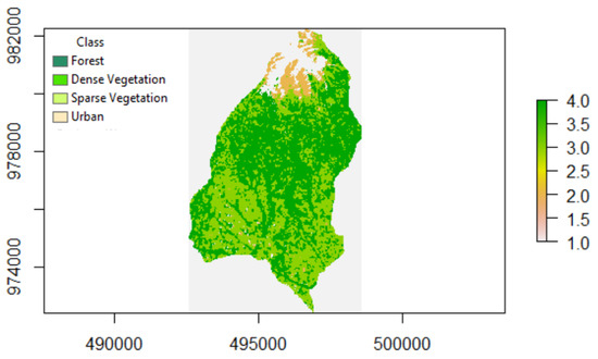
Figure 7.
The NDVI values to label the land cover.
In this study, our main objective was to build stack-based ensemble learning approach by combining multiple base classifiers. The main purpose of the stacking approach was to further optimize classification performance by combining the base classifiers. Stack-based method is a potentially capable enough to handle complex data such as raster image data. Consequently, the proposed model outperformed all the individual base classifiers and produced the highest classification accuracy. We have conducted a comparison analyses between the performance of our proposed methods and state-of-the-art machine learning models in similar domain areas. Table 6 summarize comparative data.
It is clear from Table 7 that several attempts have been made to improve classification performance in the domain of hyper-spectral image processing. A number of ensemble learning methods have been proposed to analyze land cover and land use using image data. Our proposed Stacked-XGBoost model outperformed other models and it is efficient enough to handle multi-spectral image data.
Table 7.
Summary of performance by ensemble learning models.
6. Summary and Conclusions
The purpose of the present work was to develop an effective method for accurate land use/land cover (LULC) classification to efficiently utilize scarce natural resources and to design a mechanism for precision agriculture. Well-designed machine learning method can address the limitations of current labor-intensive and time-consuming processes. In addition, getting high resolution multi-spectral image data is a critical challenge in the Ethiopian context. Despite image resolution, the process of labeling training and collecting representative sample data were a tricky task. During model building, we observed that most of the base classifiers suffer from an inability to handle complex and non-linear hyper-spectral image data. This is due to the high-dimensionality of Landsat images that contain hundreds and thousands of feature bands, mixed pixel values, dark-object on the surface of the earth, and limitation of feature extraction, and others.
Therefore, we proposed a stack-based ensemble learning method to classify hyper-spectral image data collected from a location in Ethiopia. The performance level of the proposed model exceeded that of individual base classifier. Furthermore, integrating ensemble learning methods can potentially lead to capable of handling complex hyper-spectral image data.
Based on our findings, we can conclude that, ensemble-based approaches outperform any strong single machine learning algorithm. However, there are many issues in the domain area that need further exploration. First, in the case of Ethiopia, obtaining satellite data with less than 10 m resolution is a big challenge. To conduct high-level domain specific research such as precision agriculture, image resolution and its quality are critical factors when making the final decision. Second, we employed small-size observations to fit the model. Small size and imbalance of training samples were the causes leading to model over-fitting. A semi-supervised features extraction can be a possible solution to obtain representative feature to enhance models’ classification performance. Finally, model sensitivity needs further exploration in multi-spectral image classification. To handle the pitfalls, currently we are working on an ensemble of deep-learning to classify hyper-spectral image data. Combining the feature extraction capabilities with deep-learning ensemble approaches could resolve the above-mentioned bottle-necks.
Author Contributions
Conceptualization, T.A. and A.R.; methodology, T.A.; software, T.A.; validation, A.R., T.A. and R.S.; formal analysis, T.A. and A.R.; investigation, T.A.; resources, T.A.; data curation, T.A.; writing—original draft preparation, T.A.; writing—review and editing, T.A., A.R. and R.S.; visualization, T.A.; supervision, A.R. and R.S.; project administration, R.S. All authors have read and agreed to the published version of the manuscript.
Funding
There is no funding organization or institutional support to conduct the current study. But, MDPI Editorial Board provide us a grant of waivers and 100% discounts on this article publishing charges (APCs).
Institutional Review Board Statement
Not applicable.
Informed Consent Statement
Not applicable.
Data Availability Statement
The multi-spectral image classification experimental output and sample code will be uploaded on my Github repository which is located at https://github.com/tagel123/Multi-Spectral-Image-Classification/ (accessed on 1 December 2021). But, our data-set size is more than 3 GB which beyond the limitation of git-hub. To resolve this challenge connect the git with google drive to make the data public available.
Acknowledgments
First, we thank Abebe Rorrisa for his enormous support and advice. Then, we thank Ramasamy for his contribution to my pursuit of PhD work. Finally, we thank all of the supporter who directly or indirectly participated in this research study. MDPI technology editorial board allow fund for waiving the journal publication charges. We deeply appreciate the opportunities given by the MDPI journal editorial boards.
Conflicts of Interest
The authors declare that, there is no conflict of interest to public the manuscript. We acknowledge the data sources and cite all the references which used to prepare the manuscript. We would also like to acknowledge MDPI Editorial board support their financial support by waiving publication charge. Finally, A complete or partial parts of this study report haven’t submitted or published on any platform. “The funders had no role in the design of the study; in the collection, analyses, or interpretation of data; in the writing of the manuscript; or in the decision to publish the results.
Abbreviations
The following abbreviations are used in this manuscript:
| AVIRIS | Airborne Visible Infrared Imaging Spectrometer |
| BARI | Bishoftu Agricultural Research Institute |
| B2 | Blue Band |
| B3 | Green Band |
| B4 | Red Band |
| CV | Computer Vision |
| CNN | Convolutional Neural Network |
| DSNN | Deep Stack Neural Network |
| EWS | Early Warning System |
| FCC | False Color Composite |
| FE | Feature Extraction |
| KNN | K-Nearest Neighbor |
| KELM | Kernel based Extreme Learning Machine |
| LCLU | Land cover Land Use |
| NDVI | Normalized Difference Vegetation Index |
| NIR | Near Infrared Band |
| NWFE | Non-parameteric Weighted Feature Extraction |
| PA Precision Agriculture | |
| RF | Random Forest |
| RMG | Random Multi-Graph |
| RIO | Region Of Interest |
| ROSIS | Reflective Optics System Imaging Spectrometer |
| SVM | Support Vector Machine |
| XGBoost | Extreme Gradient Boosting |
References
- Eshetu, A.A. Forest resource management systems in Ethiopia: Historical perspective. Int. J. Biodivers. Conserv. 2014, 6, 121–131. [Google Scholar]
- Hanuschak Sr, G.A. Timely and accurate crop yield forecasting and estimation: History and initial gap analysis. In The first Scientific Advisory Committee Meeting, Global Strategy; Food and Agriculture Organization of the United Nations: Rome, Italy, 2013; Volume 198. [Google Scholar]
- Knickel, K.; Ashkenazy, A.; Chebach, T.C.; Parrot, N. Agricultural modernization and sustainable agriculture: Contradictions and complementarities. Int. J. Agric. Sustain. 2017, 15, 575–592. [Google Scholar] [CrossRef]
- Kamilaris, A.; Prenafeta-Boldú, F.X. Deep learning in agriculture: A survey. Comput. Electron. Agric. 2018, 147, 70–90. [Google Scholar] [CrossRef] [Green Version]
- Abdullahi, H.; Zubair, O.M. Advances of image processing in precision agriculture: Using deep learning convolution neural network for soil nutrient classification. J. Multidiscip. Eng. Sci. Technol. (Jmest) 2017, 4, 7981–7987. [Google Scholar]
- Anandhakrishnan, T.; Jaisakthi, S. Internet of Things in Agriculture-Survey. J. Comput. Theor. Nanosci. 2018, 15, 2405–2409. [Google Scholar] [CrossRef]
- Kumar, N.; Vidyarthi, D.P. A green routing algorithm for IoT-enabled software defined wireless sensor network. IEEE Sens. J. 2018, 18, 9449–9460. [Google Scholar] [CrossRef]
- Araby, A.A.; Abd Elhameed, M.M.; Magdy, N.M.; Abdelaal, N.; Abd Allah, Y.T.; Darweesh, M.S.; Fahim, M.A.; Mostafa, H. Smart iot monitoring system for agriculture with predictive analysis. In Proceedings of the 2019 8th International Conference on Modern Circuits and Systems Technologies (MOCAST), Thessaloniki, Greece, 13–15 May 2019; pp. 1–4. [Google Scholar]
- Dubey, S.R.; Jalal, A.S. Apple disease classification using color, texture and shape features from images. Signal Image Video Process. 2016, 10, 819–826. [Google Scholar] [CrossRef]
- Mavridou, E.; Vrochidou, E.; Papakostas, G.A.; Pachidis, T.; Kaburlasos, V.G. Machine vision systems in precision agriculture for crop farming. J. Imaging 2019, 5, 89. [Google Scholar] [CrossRef] [Green Version]
- Aboneh, T.; Rorissa, A.; Srinivasagan, R.; Gemechu, A. Computer Vision Framework for Wheat Disease Identification and Classification Using Jetson GPU Infrastructure. Technologies 2021, 9, 47. [Google Scholar] [CrossRef]
- Mateen, M.; Wen, J.; Nasrullah; Akbar, M.A. The role of hyperspectral imaging: A literature review. Int. J. Adv. Comput. Sci. Appl. 2018, 9, 51–62. [Google Scholar]
- Kale, K.V.; Solankar, M.M.; Nalawade, D.B.; Dhumal, R.K.; Gite, H.R. A research review on hyperspectral data processing and analysis algorithms. Proc. Natl. Acad. Sci. India Sect. Phys. Sci. 2017, 87, 541–555. [Google Scholar] [CrossRef]
- Jahan, F.; Zhou, J.; Awrangjeb, M.; Gao, Y. Inverse coefficient of variation feature and multilevel fusion technique for hyperspectral and LiDAR data classification. IEEE J. Sel. Top. Appl. Earth Obs. Remote. Sens. 2020, 13, 367–381. [Google Scholar] [CrossRef] [Green Version]
- Merentitis, A.; Debes, C.; Heremans, R. Ensemble learning in hyperspectral image classification: Toward selecting a favorable bias-variance tradeoff. IEEE J. Sel. Top. Appl. Earth Obs. Remote. Sens. 2014, 7, 1089–1102. [Google Scholar] [CrossRef]
- Paoletti, M.; Haut, J.; Plaza, J.; Plaza, A. Deep learning classifiers for hyperspectral imaging: A review. Isprs J. Photogramm. Remote. Sens. 2019, 158, 279–317. [Google Scholar] [CrossRef]
- Maulik, U.; Chakraborty, D. A self-trained ensemble with semisupervised SVM: An application to pixel classification of remote sensing imagery. Pattern Recognit. 2011, 44, 615–623. [Google Scholar] [CrossRef]
- Fang, L.; Zhao, W.; He, N.; Zhu, J. Multiscale CNNs Ensemble Based Self-Learning for Hyperspectral Image Classification. IEEE Geosci. Remote. Sens. Lett. 2020, 17, 1593–1597. [Google Scholar] [CrossRef]
- Ergul, U.; Bilgin, G. Multiple-instance ensemble learning for hyperspectral images. J. Appl. Remote. Sens. 2017, 11, 045009. [Google Scholar] [CrossRef]
- Lv, F.; Han, M.; Qiu, T. Remote sensing image classification based on ensemble extreme learning machine with stacked autoencoder. IEEE Access 2017, 5, 9021–9031. [Google Scholar] [CrossRef]
- Gao, F.; Wang, Q.; Dong, J.; Xu, Q. Spectral and spatial classification of hyperspectral images based on random multi-graphs. Remote. Sens. 2018, 10, 1271. [Google Scholar] [CrossRef] [Green Version]
- Ceamanos, X.; Waske, B.; Benediktsson, J.A.; Chanussot, J.; Fauvel, M.; Sveinsson, J.R. A classifier ensemble based on fusion of support vector machines for classifying hyperspectral data. Int. J. Image Data Fusion 2010, 1, 293–307. [Google Scholar] [CrossRef] [Green Version]
- Koziarski, M.; Krawczyk, B.; Woźniak, M. The deterministic subspace method for constructing classifier ensembles. Pattern Anal. Appl. 2017, 20, 981–990. [Google Scholar] [CrossRef] [Green Version]
- Chen, Y.; Zhao, X.; Lin, Z. Optimizing subspace SVM ensemble for hyperspectral imagery classification. IEEE J. Sel. Top. Appl. Earth Obs. Remote Sens. 2014, 7, 1295–1305. [Google Scholar] [CrossRef]
- Samat, A.; Li, E.; Wang, W.; Liu, S.; Lin, C.; Abuduwaili, J. Meta-XGBoost for hyperspectral image classification using extended MSER-guided morphological profiles. Remote Sens. 2020, 12, 1973. [Google Scholar] [CrossRef]
- Colkesen, I.; Kavzoglu, T. Performance evaluation of rotation forest for svm-based recursive feature elimination using Hyper-spectral imagery. In Proceedings of the 2016 8th Workshop on Hyperspectral Image and Signal Processing: Evolution in Remote Sensing (WHISPERS), Los Angeles, CA, USA, 21–24 August 2016; pp. 1–5. [Google Scholar]
- Xia, J.; Yokoya, N.; Iwasaki, A. Hyperspectral image classification with canonical correlation forests. IEEE Trans. Geosci. Remote Sens. 2016, 55, 421–431. [Google Scholar] [CrossRef]
- Juang, C.; Hsieh, C. Fuzzy C-means based support vector machine for channel equalisation. Int. J. Gen. Syst. Taylor Fr. 2009, 38, 273–289. [Google Scholar] [CrossRef]
- Uddin, M.P.; Mamun, M.A.; Hossain, M.A. PCA-based feature reduction for hyperspectral remote sensing image classification. IETE Tech. Rev. 2021, 38, 377–396. [Google Scholar] [CrossRef]
- Parshakov, I.; Coburn, C.; Staenz, K. Z-Score distance: A spectral matching technique for automatic class labelling in unsupervised classification. In Proceedings of the 2014 IEEE Geoscience and Remote Sensing Symposium, Quebec City, QC, Canada, 13–18 July 2014; pp. 1793–1796. [Google Scholar]
- Zhong, G.; Liu, C.L. Error-correcting output codes based ensemble feature extraction. Pattern Recognit. 2013, 46, 1091–1100. [Google Scholar] [CrossRef]
- Chen, C.; Li, W.; Su, H.; Liu, K. Spectral-spatial classification of hyperspectral image based on kernel extreme learning machine. Remote Sens. 2014, 6, 5795–5814. [Google Scholar] [CrossRef] [Green Version]
- Pan, B.; Shi, Z.; Xu, X. Hierarchical guidance filtering-based ensemble classification for hyperspectral images. IEEE Trans. Geosci. Remote Sens. 2017, 55, 4177–4189. [Google Scholar] [CrossRef]
- Qi, C.; Zhou, Z.; Wang, Q.; Hu, L. Mutual information-based feature selection and ensemble learning for classification. In Proceedings of the 2016 international conference on identification, information and knowledge in the internet of things (IIKI), Beijing, China, 20–21 October 2016; pp. 116–121. [Google Scholar]
- Li, F.; Xu, L.; Siva, P.; Wong, A.; Clausi, D.A. Hyperspectral image classification with limited labeled training samples using enhanced ensemble learning and conditional random fields. IEEE J. Sel. Top. Appl. Earth Obs. Remote Sens. 2015, 8, 2427–2438. [Google Scholar] [CrossRef]
- Xia, J.; Bombrun, L.; Berthoumieu, Y.; Germain, C.; Du, P. Spectral–spatial rotation forest for hyperspectral image classification. IEEE J. Sel. Top. Appl. Earth Obs. Remote Sens. 2017, 10, 4605–4613. [Google Scholar] [CrossRef] [Green Version]
- Yang, J.M. Applying a dynamic subspace multiple classifier for remotely sensed hyperspectral image classification. In Proceedings of the 2012 IEEE International Geoscience and Remote Sensing Symposium, Munich, Germany, 22–27 July 2012; pp. 4142–4145. [Google Scholar]
- Yoon, Y.; Durand, M.; Merry, C.J.; Rodríguez, E. Improving temporal coverage of the SWOT mission using spatiotemporal kriging. IEEE J. Sel. Top. Appl. Earth Obs. Remote. Sens. 2013, 6, 1719–1729. [Google Scholar] [CrossRef]
- Qu, Y.; Qi, H. uDAS: An untied denoising autoencoder with sparsity for spectral unmixing. IEEE Trans. Geosci. Remote Sens. 2018, 57, 1698–1712. [Google Scholar] [CrossRef]
- Wang, Y.; Mei, J.; Zhang, L.; Zhang, B.; Zhu, P.; Li, Y.; Li, X. Self-supervised feature learning with CRF embedding for hyperspectral image classification. IEEE Trans. Geosci. Remote Sens. 2018, 57, 2628–2642. [Google Scholar] [CrossRef]
- Yuan, Q.; Zhang, Q.; Li, J.; Shen, H.; Zhang, L. Hyperspectral image denoising employing a spatial–spectral deep residual convolutional neural network. IEEE Trans. Geosci. Remote Sens. 2018, 57, 1205–1218. [Google Scholar] [CrossRef] [Green Version]
- Xia, J.; Ghamisi, P.; Yokoya, N.; Iwasaki, A. Random forest ensembles and extended multiextinction profiles for hyperspectral image classification. IEEE Trans. Geosci. Remote Sens. 2017, 56, 202–216. [Google Scholar] [CrossRef] [Green Version]
- Chen, T.; Guestrin, C. XGBoost: A Scalable Tree Boosting System. In Proceedings of the22nd ACM SIGKDD International Conference on Knowledge Discovery and Data Mining (KDD’16), San Francisco, CA, USA, 13–17 August 2016; pp. 785–794. [Google Scholar]
- Zhao, F.; Lin, F.; Seah, H.S. Bagging based plankton image classification. In Proceedings of the 2009 16th IEEE International Conference on Image Processing (ICIP), Cairo, Egypt, 7–10 November 2009; pp. 2081–2084. [Google Scholar]
- Novakovic, J. Bagging algorithm for pixel classification. In Proceedings of the 2011 19th Telecommunications Forum (TELFOR) Proceedings of Papers, Belgrade, Serbia, 22–24 November 2011; pp. 1348–1351.
- Feng, W.; Huang, W.; Bao, W. Imbalanced hyper-spectral image classification with an adaptive ensemble method based on smote and rotation forest with differentiated sampling rates. IEEE Geosci. Remote Sens. Lett. 2019, 16, 1879–1883. [Google Scholar] [CrossRef]
Publisher’s Note: MDPI stays neutral with regard to jurisdictional claims in published maps and institutional affiliations. |
© 2022 by the authors. Licensee MDPI, Basel, Switzerland. This article is an open access article distributed under the terms and conditions of the Creative Commons Attribution (CC BY) license (https://creativecommons.org/licenses/by/4.0/).