1. Introduction
A reverse mortgage is a scheme wherein senior citizens who are owner-occupiers of houses can receive fixed monthly instalments in the form of pensions (
Han et al. 2017). In other words, a reverse mortgage is a loan secured against the home equity owned by the borrower (
Kutty 1998). The phenomenon of aging societies in developed countries and low-interest rate environments are contributing to serious problems with pension systems. Due to these issues, the importance of reverse mortgage products is increasing, as they can guarantee the income of the elderly (
Knaack et al. 2020). Similar banking loans related to mortgages have been available since 1995, but these were initially not popular in Korea due to limited loan periods and fairly high interest rates. The formal reverse mortgage was introduced into the market after 2007; the market reaction, however, was somewhat lackluster. A rapid increase in this market started in 2014, when Korean house owners became more interested in this product due to reverse mortgages being highlighted on local news media, and lower market interest rates
1. Korea is facing a significant challenge in population aging. The ratio of Korean citizens who are older than 65 the total Korean population has been rising rapidly, from 7.2% in 2000 to 14.9% in 2019. This ratio is expected to increase even further to 46.5% by 2067, according to Statistics Korea. The global ratio of over 65s was 9.1% in 2019, and is expected to increase to 18.6% by 2067, according to the UN. This is one of key factors promoting reverse mortgages in Korea.
Reverse mortgages were first established as an instrument to provide cash flow for senior citizens without a regular income.
Chinloy and Megbolugbe (
1994) argued that they were developed for a contract where the borrower receives monthly payments, while the loan balance is accumulated as a claim against the house price. In general, a reverse mortgage is a scheme that can be formulated as a form of put option in which the house value becomes the underlying asset, and total payments received become the exercise price (
Merrill et al. 1994). Indeed, many empirical studies have demonstrated that reverse mortgage programs may enhance a stable residential and senior life (
Kutty 1998;
Ong 2008). Therefore, a reverse mortgage is a long-term financial product with many linkage risks, due to the uncertainty of market dynamics (
Chinloy and Megbolugbe 1994). Under reverse mortgage schemes, financial institutions face the risk of variations in housing prices
2. On the other hand, borrowers could acquire the option value embedded in a reverse mortgage despite variations in house prices. In particular, Korean reverse mortgages have been designed as a form of long position in both the call option and the put option of the European option, unlike reverse mortgage products in Hong Kong
3 (
Han et al. 2017). These characteristics are one of the crucial reasons for the popularity of the Korean reverse mortgage market, because Korean reverse mortgages have a straddle strategy, which provides a hedge strategy for consumers. Therefore, Korean reverse mortgages are a very attractive product for borrowers, because they can receive a regular cash flow to cover living expenses without being affected by market risk, such as house price variations. In particular, borrowers do not have to repay anything within this scheme, even if the total amount borrowed exceeds the house price, which is called a non-recourse loan. In addition, if the house price is higher than the total outstanding balance, the heirs can inherit the house and have the asset value of the asset to aid in repaying the loan balance.
4The aim of this paper was to examine specific market values through option matching from the borrower perspective. This study explores the option value of a reverse mortgage in Korea, through an empirical analysis using the Black–Scholes option-pricing model within the proven
Han et al. (
2017) research framework.
Han et al. (
2017) examined the put option value of reverse mortgages in Hong Kong, focusing on the non-recourse value of the reverse mortgage. They showed specific monetary values through option matching from the borrower perspective. In addition to
Han et al. (
2017), we present the possible call option value in this paper, when the house price exceeds the threshold price.
This paper found the following results. First, the call option value is 5.8% of the house price at the age of 60, under the assumption of a KRW (Korean Won) three hundred million house value, while the put option value is only 2.0%. Only the call option value remains at the age of 80. Second, this article analyzed the sensitivity of the key variables of real-option analytical models, such as exercise price, the risk-free rate, volatility, and maturity, on the option value of a reverse mortgage. The sensitivity results of the key variables support economic rationales for the option pricing model.
The remainder of this paper is organized as follows.
Section 2 reviews the major literature on this subject.
Section 3 describes our estimation methodology, and
Section 4 presents the empirical results, sensitivity analyzes according to the option model, and the values of the options. The summary and conclusions are given in
Section 5.
2. Literature Review
The literature on reverse mortgage loans is growing rapidly. In the theoretical area, work has been presented by
Chinloy and Megbolugbe (
1994),
Miceli and Sirmans (
1994),
Bardhan et al. (
2006),
Nakajima and Telyukova (
2017), and many others.
Chinloy and Megbolugbe (
1994) introduced the pricing model for a reverse mortgage contract, where the borrower receives payments either as a lump sum or in an annuity while the loan balance accumulates as a claim against the house.
Miceli and Sirmans (
1994) developed a theoretical model of the problem of maintenance risk in reverse mortgages. The results of the model showed that lenders would respond to the problem either by limiting the amount of reverse mortgage loans to guarantee that maintenance risk was not a threat, or by charging an interest rate premium to cover the expected cost of default.
Bardhan et al. (
2006) developed a redeemable reverse mortgage loan-pricing model under European put options, where agents were risk neutral. They argued that the model would be useful in emerging market economies.
Nakajima and Telyukova (
2017) analyzed mortgages in a calibrated life-cycle model of retirement, considering their future following the great recession. The model predicted that the ex-ante welfare benefit of reverse mortgages was equivalent to providing a lump-sum transfer of
$252 per retired homeowner at the age of 65.
There are also several empirical studies into reverse mortgages, including those by
Merrill et al. (
1994),
Kutty (
1998),
Ong (
2008),
Donald et al. (
2013), and many others.
Merrill et al. (
1994) used American Housing Survey (AHS) data to estimate the potential size of the market for unrestricted reverse mortgages. They found that the reverse mortgage was a very attractive product to borrowers, because they could receive cash flow to cover living expenses. They also used the 1985 through 1988 AHS Standard Metropolitan Statistical Area (SMSA) Surveys to identify areas that had a large number of senior homeowners in the prime target group.
Kutty (
1998) utilized data from National File within the American Housing Survey of 1991. She estimated that the poverty rate of elderly households in occupied units could be reduced by three percent (from 17% to 14%) by means of reverse mortgages.
Ong (
2008) investigated the extent to which reverse mortgages could improve the economic welfare of elderly Austrian homeowners. She found that the scope for reverse mortgages to improve economic welfare was considerable.
Donald et al. (
2013) examined an empirical analysis of the influence of house price dynamics on reverse mortgage loan demand. They found that sellers switch to an auction-like model during housing market booms, while sellers’ list prices were sticky during a downturn in the housing market.
There have been several meaningful contributions to theoretical calculations around reverse mortgages.
Wang et al. (
2016) presented a closed-form formula for calculating the loan-to-value (LTV) ratio in an adjusted-rate reverse mortgage.
Tsay et al. (
2014) drove an approximate pricing formula for use in reverse mortgage valuation.
Shao et al. (
2015) analyzed the combined impact of house price risk and longevity risk of reverse mortgages. Their model incorporated a new hybrid hedonic-repeat-sales pricing model, as well as a stochastic mortality model for mortality improvements.
Li et al. (
2019) provided a Bayesian multivariate approach for pricing a reverse mortgage.
Lee et al. (
2012) proposed an analytic valuation framework with mortality risk, interest rate risk, and housing price risk that helped determine fair premiums. More than 80% of the assets held by seniors are real estate, according to Statistics Korea. Therefore, they tend to need more cash assets for consumption after retirement. On the other hand, the income replacement rate of the national pension is only 45%, which is not sufficient to guarantee the retirement wellbeing of the seniors. The reverse mortgage can be a good way to overcome this problem.
4. Empirical Results and Discussion
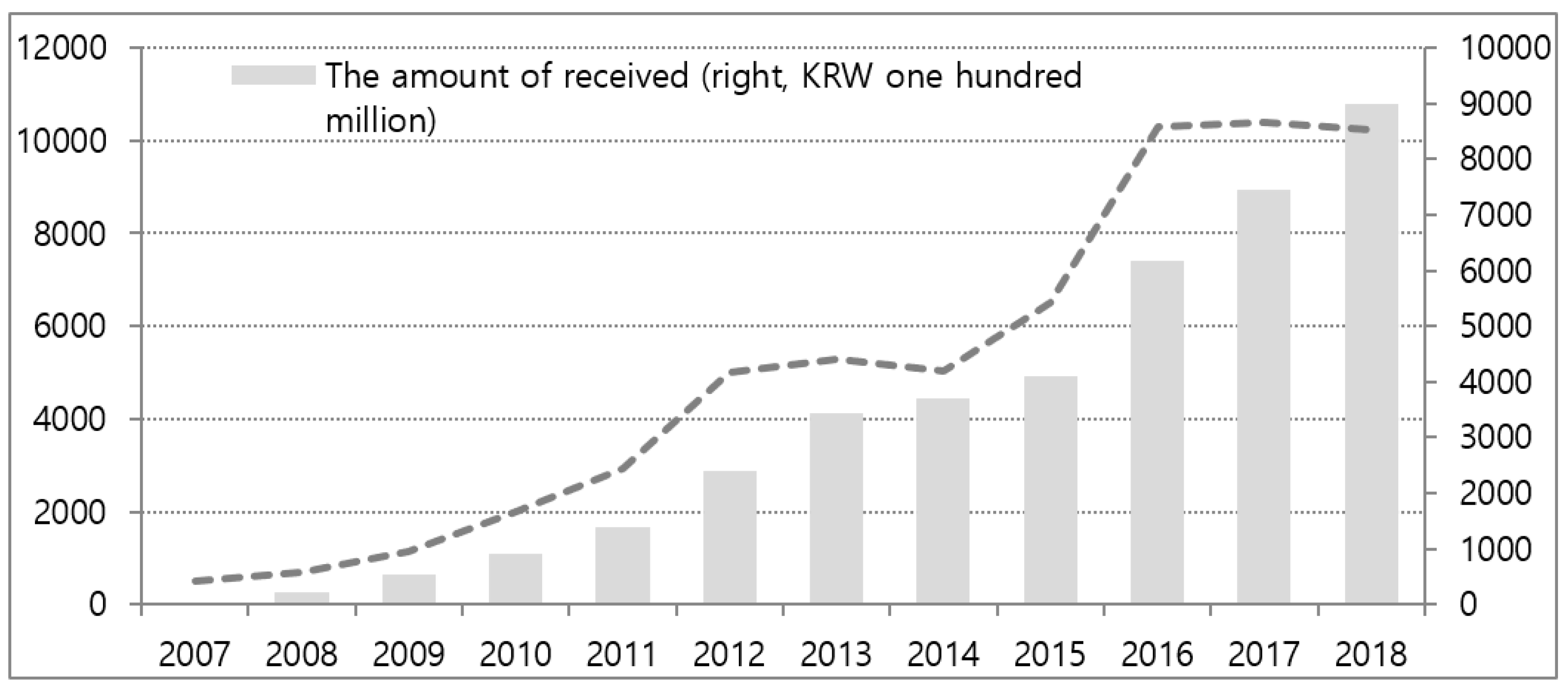
Figure 1 displays the overall trend of the total number of borrowers in Korea, and the amount of reverse mortgage loan periods from 2007 to 2018. The number of mortgages was small before 2011, but has been gradually growing since then. At the end of 2018, the number of mortgages exceeded 60,000. We believe that the number will continually grow going forward.
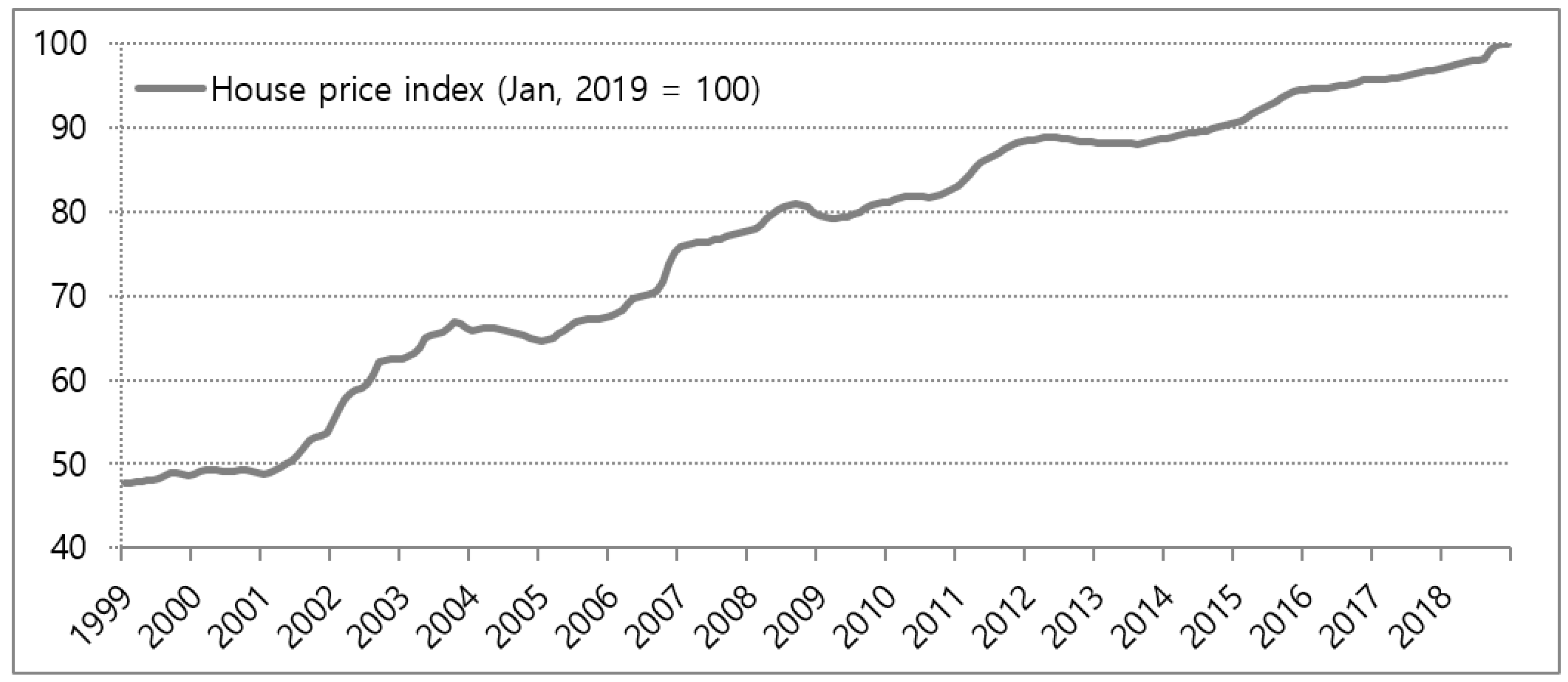
In this study, we selected the house price index in Korea from January 1999 to December 2018.
Figure 2 shows that the housing price trend is increasing, with continuous random variables subject to the GBM process for the long term, which is similar to the Definitive Real Estate Price Indices of Hong Kong (
Han et al. 2017).
4.1. Main Results of Option Pricing Estimation
Table 3 reports the estimated option prices by age group and house price level. Overall, the call option value increases as age increases, while the put option value decreases in Panel A. For example, an applicant at the age of 60 has a KRW 17.7 hundred million call option value and a KRW 5.8 hundred million put option value under the assumption of a 25 year lifespan. On the other hand, an applicant at the age of 80 has a KRW 95.9 hundred million call option value and no put option value.
Panel B reports the value of the call option and put option in which the calculated option prices are divided by the underlying house prices. Overall, the call option value rises as the age of the applicant rises. On the other hand, there are no put option values for age 75 and age 80. The value of the call option and the value of the put option enjoyed by a 60-year-old applicant of a reverse mortgage, who owns a house worth KRW three hundred million, are 5.9% and 1.9%, respectively. On the other hand, the value of the put option is zero for an 80-year-old, while the value of the call option is 32.0%. These are the typical characteristics of a reverse mortgage, wherein the residual life expectancy is different. An applicant at the age of 80 maintains the call option (in-the-money) at the termination date of the reverse mortgage. This study found that when the applicant age is lower, the benefit of a reverse mortgage is greater. In this case, it is an attractive financial program that can partially resolve the financial issues of the senior citizens.
4.2. Exercise Price Sensitivity Analysis
To determine the influence of key parameters on the option value of a reverse mortgage, such as the exercise price (
), risk-free rate (
), volatility (
), and maturity (
), this article analyzes the sensitivity of variables of real-option analytical models based on the option value of a reverse mortgage. Volatility is the most important variable in the real option calculation, as it represents the level of uncertainty (
Han et al. 2017). If volatility is higher, the value of the option increases.
Notice that the exercise price is the total amount of outstanding balance calculated at the maturity of the reverse mortgage, based on the previous monthly payment, insurance fee, and interest rate expense. The interest rate expense depends upon the CD (Certificate of Deposit) rate or COFIX (Cost of Fund Index) rate. As the CD rate increases, the call option value decreases but the put option value increases.
Table 4 shows the sensitivity of the option value according to the change in CD rate. Based on the result, the call option value decreases due to a rise in the CD rate, while the put option value increases regardless of the age difference. At the age of 80, the CD rate rises to 10%, which increases the put option value and the call value by 0.1% and 9.8%, respectively. On the other hand, the CD rate stays at 0.1%, which generates the call option value and the put option values of 48.4% and 0.0%, respectively. At the age of 60, however, the valuation of the option value in terms of the change in the CD rate is somewhat larger compared to that at the age of 80.
Figure 3 shows the sensitivity of the option value according to the change in CD rate from 0.1% to 10%. In Panel A, the call option value decreases at the age of 60. The intersection point between the call option value line and the put option value line is at 5.5% of the CD rate; the put option value increases from then. On the other hand, at the age of 80, the put option value line shows no change, while the call option value line decreases as the CD rate increases.
4.3. Risk-Free Rate Sensitivity Analysis
Table 5 shows the sensitivity of the option value according to the change in the risk-free rate
5. It was found that there is a positive relationship between the risk-free rate and the call option value, while there is a negative relationship between the risk-free rate and put option value. The present value of the exercise price falls as the risk-free rate rises, which implies that the call option value increases but the put option value decreases as the risk-free rate rises.
Based on
Table 6, regardless of applying at age 60 or at age 80, the call option value increases as the risk-free rate rises, while the put option value decreases. In particular, a risk-free rate below 3% changes only the put option value, while a risk-free rate over 3% causes variation in only the call option value.
The risk-free rate stays at 0.1%, which puts the put option value at 49.9% of the house price at age 60 and 0.0% of the house price at age 80, respectively. As the risk-rate rises to 12%, the call option value increases to 93.3% of the house price at age 60 and 75.4% of the house price at age 80. Hence, the variations of the call option value and the put option value at 60 are somewhat larger compared to those of the call option value and the put option value at age 80.
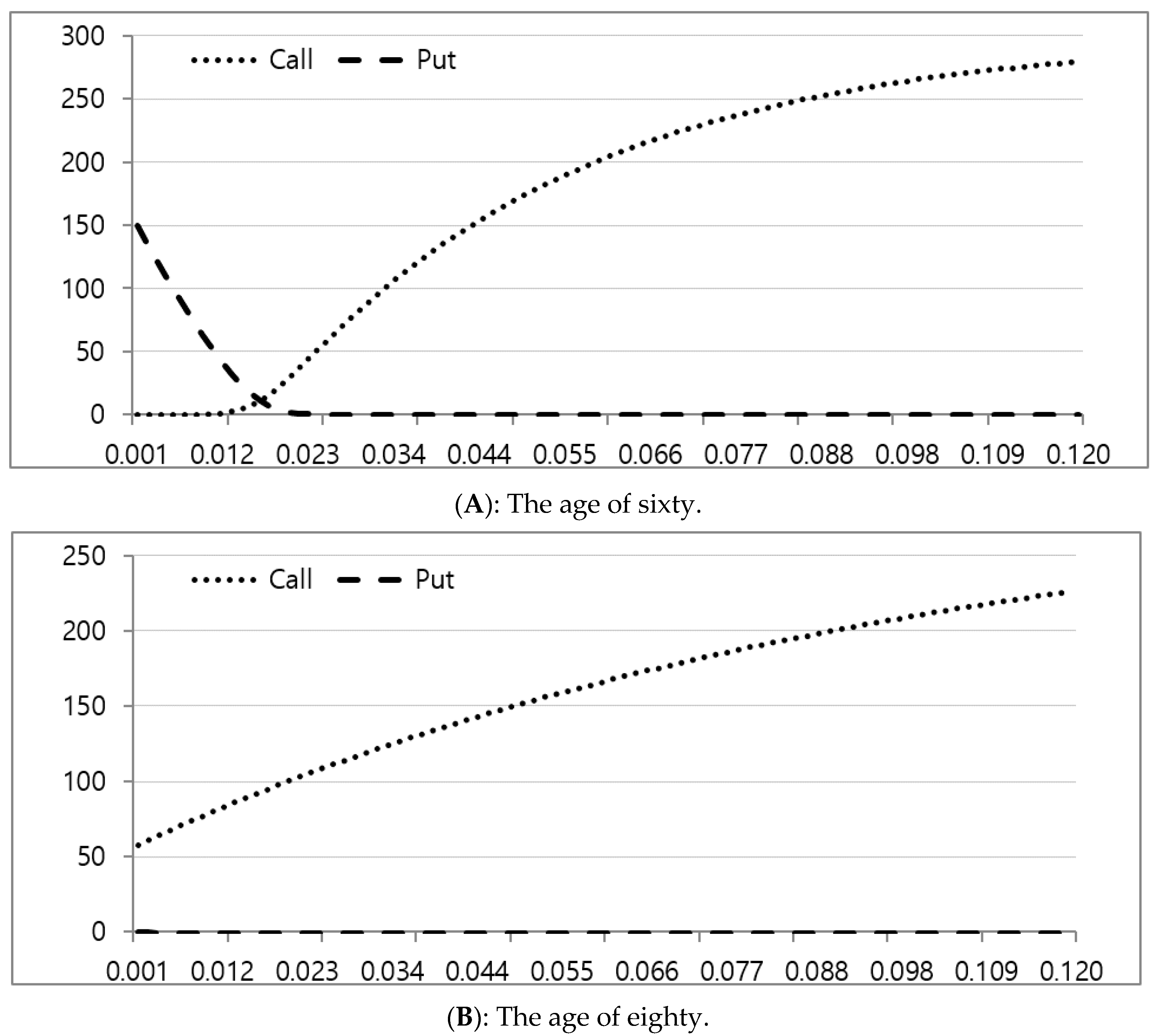
Figure 4 exhibits the sensitivity of the option value according to a change in the risk-free rate from 0.1% to 12%. In Panel A, the put option value decreases at age 60 as the risk-free rate rises. The intersection point between the call option value line and the put option value line is at 1.5% of the risk-free rate, since then only the call option value line increases. On the other hand, at age 80, the put option value line shows virtually no change, while the call option value line increases as the risk-free rate falls.
4.4. House Price Sensitivity Analysis
Table 6 examines the sensitivity of the option value according to the change in house price. There is a positive relationship between the underlying asset (house price) volatility and the option value. Hence, both the call option value and the put option value rise as the underlying asset volatility increases. Based on
Table 7, both at age 60 and at age 80, the option values of both the call and put options increase as the underlying asset volatility rises. In particular, the volatility of the underlying asset at age 60 stays at only 0.0001 and does not have a put option value, but other volatilities have the call option value and the put option value. At age 80, the volatility of the underlying asset reaches 0.0151, which is the starting point of the put option in value. In general, the option value of both the call and put at age 60 is somewhat larger compared to that of the call and put at age 80.
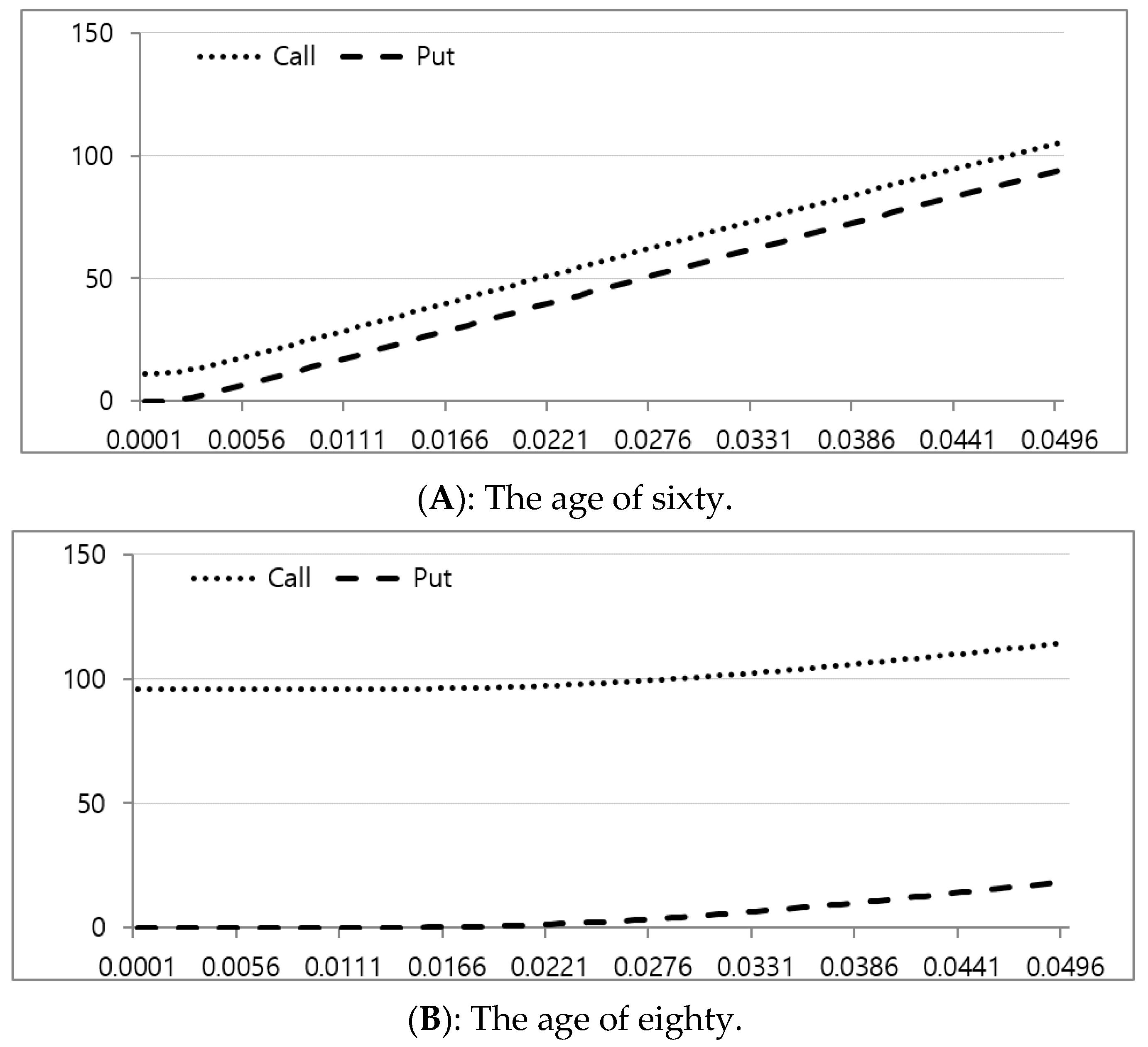
Figure 5 shows the sensitivity of the call option value and the put option value according to the change in the underlying asset volatility under the assumption of a KRW three hundred million house value; the underlying asset volatility changes from 0.0001 to 0.0496. At age 60 (Panel A) and at age 80 (Panel B), the call option value and the put option value increase as the underlying volatility rises. At age 80, the option value increases since the underlying asset volatility is over 0.0221, which is somewhat larger compared to what it is at age 60.
4.5. Maturity Sensitivity Analysis
Finally, we examined the sensitivity of the option value to a change in maturity. The reverse mortgage has monthly instalments which reflect the expected lifetime span. However, the expected lifetime of the borrower is unknown, which effects the maturity and eventually the option price.
Table 7 shows the option value of both the call and the put as the maturity changes to 100 years old. The option values of both the call and the put increase as maturity rises. Based on
Table 7, the call option value at age 60 decreases as maturity rises, and it has virtually no value from 288 months (24 years). However, the put option value at age 60 remains stable from 288 months. On the other hand, the call option value at age 80 decreases as maturity rises, and the put option value increases from 192 months (16 years). The option value has a different structure from the call and put as maturity changes. Notice that under the assumption of a 100 year lifespan, the put option value at age 60 is 95% of the house price, while at age 80 it is only 57.5% of the house price.
This result is in accordance with the cash flow characteristic of the borrower. The exercise price (the total loan) accumulates as maturity increases. However, there is no additional financial burden, even though the total loan is greater than the house value at the termination date (death of the borrower). It is expected that the put option value has mainly contributed to the value of the reverse mortgage, rather than the call option value, as maturity increases.
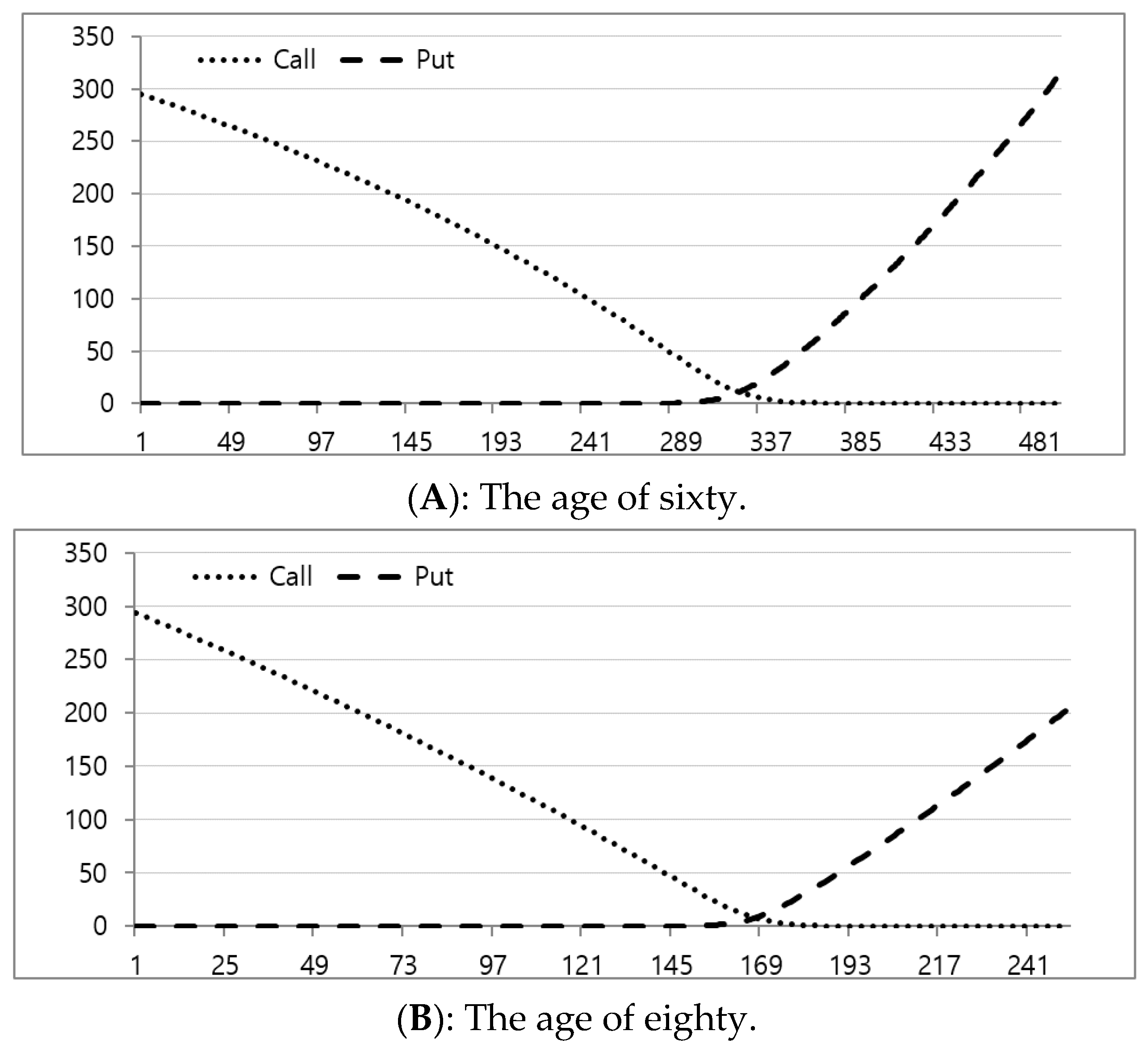
6Figure 6 explores the sensitivity of the call option value and the put option value under the assumption of a KRW three hundred house value change from the first month (initiation of the reverse mortgage) to 480 months (100 years). In Panel A, the call option value at age 60 decreases as maturity rises. The value lines of the call option and put option intersect each other at 310 months (26 years), since from this point the put option value increases substantially. In Panel B, the result at age 80 is similar to that at age 60. The call option value decreases as maturity increases. The intersection between the call option value and the put option value happens at 169 months (14 years), after that only the put option value remains.
5. Summary and Conclusions
Reverse mortgages are increasingly used as an alternative source of retirement income in Korea (
Kim and Li 2017). Reverse mortgages are also one way to mitigate the dramatic aging population problem, which threatens the social security system of Korea. The Korean government launched government-insured financial products as a reverse mortgage program through the Korea Housing Finance Corporation (KHFC). The Korean reverse mortgage program is a government guaranteed loan for elderly persons who own property and need an adequate cash flow to receive monthly instalments by collateralizing their property. The borrower is guaranteed to reside in his house and receive monthly payments for the rest of his or her life. This is critical for the success of the product. Korean reverse mortgages are similar to those of other countries. If we focus on the payoff of the borrower, this is the long position of both the European call option and put option, also known as a long straddle.
Kim and Li (
2017) argued that a Korean reverse mortgage is attractive because the homeowner receives monthly payments from the lender, with possible additional withdrawals limited by the total value of the house.
7In this paper, we analyzed the option value of the reverse mortgage in Korea through an empirical analysis, using the Black–Scholes option-pricing model. The results of our study show that, first, the call option value is 5.8% of the house price at age 60 under the assumption of a KRW three hundred million house value, while the put option value is only 2.0%. At age 80, only the call option value remains, so the option value is mainly influenced by the call option rather than the put option when the subscription to a reverse mortgage is late. Second, based upon the sensitivity of the option according to the change in exercise price, the put (call) option value increases (decreases). As the risk-free rate rises, the call (put) option value increases (decreases). The option value of both the call and put increases as the underlying asset volatility rises. In the case of maturity, the put (call) option value increases (decreases) as maturity rises. This is the reason for the characteristic of the exercise price.
This study, through sensitivity analysis of the key variables that are consistent with the general option theory, obtained results similar to those of
Han et al. (
2017) Overall, the option values of both the call and put exist as long as the borrower keeps the Korean reverse mortgage contract until the termination date. The financial value of a Korean reverse mortgage is somewhat larger when the borrower subscribes at a younger age.


