Abstract
This study investigates risk contagion and dependence structures between U.S. and Chinese technology-related stock markets, focusing on the electronics and semiconductor sectors. We employ DCC-GARCH models to capture time-varying correlations and copula models to analyze nonlinear and tail dependencies. To highlight extreme risk dynamics, we extend the analysis to Value-at-Risk (VaR) series derived from a GARCH(1,1)-Skewed-t model. Empirical results reveal three major findings. First, volatility clustering and negative skewness are evident across markets, with extreme downside risks concentrated during the 2015 Chinese stock market crash and the 2020 COVID-19 pandemic. Second, copula results show stronger upper-tail dependence in cross-border broad markets and more symmetric dependence within domestic Chinese markets, while U.S. sectoral linkages exhibit the highest vulnerability during downturns. Third, dynamic copula analysis indicates that downside contagion is episodic and crisis-driven, whereas rebound co-movements are structurally persistent. These findings contribute to understanding systemic vulnerability in global technology markets. They provide insights for investors, regulators, and policymakers on monitoring cross-market contagion and managing systemic risk under stress scenarios.
1. Introduction
1.1. Research Background
In recent years, competition in the global technology industry has intensified, with the semiconductor and electronics sectors occupying pivotal positions in both industrial supply chains and financial markets. China, leveraging a comprehensive and cost-efficient manufacturing ecosystem, holds a key position in global electronics production. The United States, by contrast, maintains dominance in the upstream semiconductor value chain through its technological innovation capacity, strong capital markets, and advanced chip fabrication technologies.
Recent studies have shown how government policies, such as the U.S. CHIPS and Science Act, have impacted the global semiconductor industry. The CHIPS Act, introduced in 2022 and extended in 2023–2024, has spurred significant investment in domestic semiconductor manufacturing, reshaping the competitive dynamics in both the U.S. and China. For instance, empirical research by Smith (2024) and Tan (2024) highlights how the CHIPS Act has altered the global semiconductor supply chain, creating both opportunities and challenges for Chinese electronics firms. This legislation has not only boosted U.S. technological leadership but also led to increased tensions in trade and technology transfer between the two countries, with profound implications for market dynamics.
Given the intertwined supply chains between the U.S. and Chinese semiconductor–electronics industries, alongside rising geopolitical tensions and tendencies toward capital market decoupling, this study examines how market interdependence and tail risk contagion manifest under both normal and extreme conditions. Specifically, we employ the DCC-GARCH model to capture time-varying correlations and the copula framework to characterize asymmetric tail dependencies during extreme market events.
Over the past decade, several pivotal events have reshaped the interdependence and competitive dynamics between the U.S. and Chinese semiconductor–electronics industries: (1) 2010–2014: Rapid expansion of China’s electronics manufacturing capacity, with state-led initiatives supporting domestic semiconductor equipment and materials. (2) 2015: Chinese stock market crash and U.S. concerns over technology transfer accelerate discussions on export control measures. (3) 2018: The U.S. imposes tariffs on Chinese electronics under Section 301 and expands restrictions on semiconductor-related exports. (4) 2019: Huawei and multiple Chinese semiconductor firms are placed on the U.S. Entity List, restricting access to critical U.S. technology. (5) 2020: COVID-19 pandemic disrupts global semiconductor supply chains, amplifying volatility in both markets. (6) 2022: The U.S. CHIPS and Science Act introduces subsidies for domestic chip manufacturing and imposes further export restrictions on advanced semiconductor technology to China. (7) 2023–2024—Intensified geopolitical tensions and expanded export controls further constrain cross-border investment and technology flows, reinforcing the trend toward supply chain bifurcation.
These events provide important context for analyzing both dynamic correlations and asymmetric tail dependencies in subsequent sections.
1.2. Research Aims
The recent sequence of geopolitical, economic, and public health shocks—from the 2015 Chinese stock market crash and the 2018–2019 U.S. trade and technology restrictions, to the COVID-19 pandemic in 2020 and the CHIPS and Science Act of 2022—has repeatedly tested the resilience and adaptability of the semiconductor–electronics supply chain. These events have not only altered trade flows and technology access but also shifted patterns of market co-movement, particularly under stress. Understanding how such shocks shape both average correlations and extreme tail dependencies is central to the present study.
1.2.1. Research Questions
This study addresses two interrelated questions: (1) Dynamic correlation—Does the correlation between the U.S. and Chinese semiconductor–electronics markets vary over time, and what factors drive these changes? (2) Tail risk dependence—During extreme market conditions (e.g., financial crises, market crashes, or heightened trade and technology restrictions), does tail dependence between these markets intensify, and does it exhibit contagion effects?
1.2.2. Research Significance
This study contributes to the literature and practice in three ways. (1) Theoretical contribution—By jointly analyzing dynamic correlations and tail risk dependencies across the U.S. and Chinese semiconductor–electronics markets, we extend existing research on international financial linkages and contagion mechanisms under extreme conditions. Our research offers novel insights into the time-varying nature of market interdependencies, especially under periods of geopolitical and economic stress. This distinction from prior work enriches the theoretical understanding of market contagion, particularly in emerging markets. (2) Policy relevance—In the face of potential geopolitical shocks and capital market decoupling, understanding risk transmission mechanisms in these industries can help policymakers design proactive measures to stabilize domestic markets. This study also contributes to recent policy debates surrounding the impact of technological sanctions and the global supply chain disruptions by providing empirical evidence on how such external shocks influence market dependencies. The empirical focus on key historical events ensures that the analysis remains grounded in realistic stress scenarios. (3) Investment implications—The results offer empirical evidence to support cross-market asset allocation, risk management, and derivative trading strategies under heightened global uncertainty. By exploring the interdependence between the U.S. and Chinese technology sectors, this study provides practical insights for investors seeking to manage risks in an increasingly interconnected global market.
1.2.3. Research Framework
This section concludes with a review of relevant literature and the theoretical framework. Section 2 then describes the data sources, summary statistics, and methodological design, emphasizing the progression from Granger causality and DCC-GARCH to copula-based dependence models. Section 3 reports the empirical evidence on dynamic correlations and tail risk linkages, and Section 4 synthesizes the key findings with policy and investment implications.
1.3. Literature Review and Theoretical Framework
1.3.1. Market Interdependence in the Technology and Electronics Sectors
The semiconductor and electronics industries are deeply embedded in global value chains, characterized by rapid innovation cycles, high capital intensity, and strong exposure to geopolitical risks. Compared with traditional industries, these sectors exhibit more volatile and asymmetric cross-country linkages due to their reliance on fragmented production networks and specialized technological capabilities. Empirical studies confirm that technology equity markets are more sensitive to global shocks, such as trade disputes or export controls, than conventional sectors (Gubareva & Strahl, 2023; Kinateder et al., 2021). Research comparing the risk dynamics between Chinese, U.S., and Eurasian markets, especially under technological sanctions, has become more prevalent. Li et al. (2022) demonstrate that while U.S. semiconductor firms face heightened volatility under trade restrictions, Chinese electronics markets experience more severe tail risks, particularly during periods of technological embargoes. This contrasts with European markets, where regulations tend to provide a moderating effect on risk spillovers (Xiong et al., 2025). In the Asian context, several studies (e.g., Allen, 2021) highlight how regional supply chain disruptions, particularly in East Asia, exacerbate these asymmetric risks, further reinforcing the need for a comparative analysis of cross-market dependence under different policy regimes.
Recent research further situates the technology sector within broader debates on innovation, supply chains, and systemic financial risks. For instance, Smith (2024) and Tan (2024) argue that global innovation-driven industries face disproportionate contagion risks because policy interventions and supply chain bottlenecks translate directly into market volatility. Similarly, Ng and Su (2025) find that shocks to technology production networks propagate asymmetrically, intensifying systemic risks in both developed and emerging markets. Moreover, recent evidence from global shocks such as the COVID-19 crisis demonstrates that systemic risk spillovers can rapidly intensify across markets, even outside the technology sector (Akhtaruzzaman et al., 2021; Akhtaruzzaman et al., 2022), reinforcing the need to examine cross-market dependencies under extreme conditions.
1.3.2. Copula Models: Theory and Applications
Copula models have become a cornerstone in modeling complex dependencies, especially in financial risk management. The concept, introduced by Sklar (1959), allows researchers to model dependencies between random variables independently of their marginal distributions. Copulas are particularly useful for capturing tail dependencies, making them ideal for risk management during extreme market events, such as crashes or booms.
Copulas enable the separation of marginal distributions from the joint distribution, allowing for flexible modeling of the dependencies between financial assets, which may exhibit nonlinear and asymmetric behaviors. The most widely used copulas in financial applications include the Gaussian copula, t-copula, Clayton copula, and Gumbel copula, each serving different types of dependencies, such as upper-tail and lower-tail dependence. Copula models have been extensively applied to model joint asset returns, especially for estimating Value-at-Risk (VaR) and Conditional Tail Expectations (CTE). For instance, Cherubini et al. (2004) applied copulas to understand joint dependencies in asset returns and measure tail risk in portfolios. Similarly, Liu et al. (2019) explored the interdependence of stock and commodity markets using copula models to assess systemic risks.
One of the key advancements in copula modeling is the introduction of dynamic copulas, such as the Dynamic Conditional Correlation (DCC) model. Unlike static copulas, dynamic copulas allow for time-varying correlations, which are crucial for modeling financial markets during periods of high volatility or systemic crises. Engle (2002) and Patton (2006) demonstrated how dynamic copulas could capture time-varying correlations in financial markets, such as those between stock markets during the 2008 financial crisis. The application of the DCC-GARCH model in this study follows this framework, capturing the time-varying dependence between U.S. and Chinese markets. Copulas are particularly valuable in tail risk management, as they allow for a more accurate representation of extreme co-movements in asset returns during market shocks. For example, Du et al. (2023) used copula models to explore the impact of systemic events, such as the COVID-19 pandemic, on market interdependence, finding that tail dependence intensifies during such crises. These models are crucial in understanding how risks propagate through interconnected markets, and they provide a better framework for portfolio diversification and hedging strategies during periods of extreme market behavior.
1.3.3. Methodological Approaches to Dependence Modeling
The empirical literature has developed a wide array of tools to measure market dependence. Linear methods, such as vector autoregression (VAR) and cointegration models, capture long-run equilibrium and short-run interactions but often miss nonlinearities and tail-specific effects. Nonlinear models, particularly the DCC-GARCH framework (Engle, 2002) and copula methods (Patton, 2006), address these limitations by allowing for time-varying correlations and asymmetric dependence structures. While DCC-GARCH models track the evolution of average correlations, copula models provide a flexible way to measure tail dependence—capturing the likelihood of extreme co-movements beyond linear correlation (Boako et al., 2019). Despite their methodological appeal, integrated applications of these models to semiconductor–electronics linkages remain limited, leaving a gap in our understanding of how structural industry interdependence manifests in financial markets.
1.3.4. Geopolitical Risk, Policy Shocks, and Market Responses
Recent work has emphasized the role of policy and geopolitical shocks in shaping market dependence. Yousaf et al. (2022) provide a detailed analysis of how U.S. semiconductor export restrictions have altered the volatility dynamics of Asian technology indices, with particular focus on the Chinese market’s exposure to U.S. policy shifts. Meanwhile, Čeryová and Árendáš (2023) report significant changes in tail dependence across regional electronics markets in Asia, Europe, and the U.S. following major policy shifts, highlighting the differing resilience levels across regions. These studies suggest that geopolitical rivalry can fundamentally reshape dependence structures by disrupting supply chains and amplifying asymmetric risks. In particular, research on how U.S.-China trade tensions have affected market linkages in the Asian market reveals a complex picture: Chinese markets show higher risk sensitivity during U.S. sanctions, while European markets tend to decouple more effectively, often with delayed risk contagion. Yet, the literature still lacks systematic analysis of how such shocks jointly affect both average correlations and extreme dependencies between U.S. and Chinese markets—the two largest players in the global semiconductor–electronics value chain.
1.3.5. Positioning Within the Broader Debate
Beyond methodological refinements, our study engages with broader academic discussions on technology-sector vulnerabilities and financial contagion. The integration of technology and electronics markets into global innovation chains implies that financial interdependence reflects not only statistical co-movements but also structural linkages rooted in production networks and strategic competition. Recent research in technological forecasting and financial risk (e.g., Smith, 2024; Tan, 2024; Ng & Su, 2025) highlights how supply chain disruptions, innovation cycles, and policy interventions disproportionately affect technology equities. Building on this line of inquiry, we conceptualize dependence structures as manifestations of both financial contagion and real-sector interdependence, making the case for combining econometric analysis with sector-specific theoretical insights.
1.3.6. Our Contribution and Research Gap
This study advances the literature in three respects. First, it examines a cross-country, cross-subsector pairing (China’s Shanghai Composite and Shenwan Electronics vs. U.S. Nasdaq Composite and Philadelphia Semiconductor) that captures both vertical supply chain linkages and strategic competition. Second, it integrates cointegration/VAR–VECM analysis with DCC-GARCH and copula models into a coherent framework linking long-run equilibrium, short-run dynamics, time-varying correlations, and tail dependence. Third, it contributes methodologically by comparing dependence structures between return series and Value-at-Risk (VaR) series for the same market pairs. While prior studies have applied copula models to returns, few have assessed whether extreme loss co-movements differ materially from average market linkages under stress conditions. By incorporating a Return Copula vs. VaR Copula comparative framework, this study disentangles the drivers of risk contagion across normal and crisis periods, thereby addressing an important empirical and theoretical gap in the literature.
2. Methods and Data
2.1. Data Sources
This study utilizes daily return data from two sector-specific indices: the PHLX Semiconductor Sector Index (Philadelphia) for the United States and the Shenwan Electronics Index (Shenwan) for China. These indices represent distinct but interconnected segments of the global electronics supply chain. The Philadelphia Index captures the upstream segment—chip design, wafer fabrication, and advanced packaging—dominated by U.S. firms with strong technological advantages and substantial global market influence. The Shenwan Electronics Index reflects the midstream and downstream segments—electronic components, optoelectronics, PCB manufacturing, and consumer electronics assembly—central to China’s role as the world’s largest electronics manufacturing base.
This upstream–downstream pairing enables the assessment of cross-border industrial linkages within the same global value chain, offering a more economically grounded perspective than pairing unrelated sectors. It also facilitates the analysis of asymmetric risk transmission channels arising from structural differences in technological leadership and manufacturing capacity.
To control for overall market movements, we include the Nasdaq Composite Index (Nasdaq) for the United States and the Shanghai Composite Index (Shanghai) for China. All price series are converted to a common currency base (USD) using daily CNY–USD exchange rates to avoid currency bias. Trading days are synchronized across markets, and non-overlapping days are removed.
Data are cross-verified from two independent sources—Wind database for China and Yahoo Finance for the United States. Descriptive statistics are computed after applying a 1% and 99% winsorization to the daily return series, mitigating the influence of extreme outliers often observed in heavy-tailed financial return distributions.
The sample spans 1 January 2005, to 13 August 2024, covering major global and bilateral events such as the Global Financial Crisis (2008), U.S.–China trade tensions (2018), the COVID-19 pandemic (2020), and the escalation of U.S. export controls on China’s technology sector in recent years.
2.2. Descriptive Statistical Analysis
Table 1 reports the descriptive statistics of daily returns for the four indices. All returns are computed as the logarithmic differences in adjusted closing prices, and winsorized at the 1% and 99% quantiles to mitigate the influence of extreme outliers and reduce the impact of heavy-tailed distributions. Before performing the statistical analysis, the raw data were sourced from Wind (for China) and Yahoo Finance (for the U.S.) and cleaned using several steps to ensure data quality and consistency.

Table 1.
Descriptive statistics of daily return.
The data cleaning process involved handling missing values, correcting inconsistencies, and eliminating any discrepancies between the data sets. Non-overlapping trading days between the U.S. and Chinese markets were removed, and daily returns were synchronized across both markets to ensure accurate comparison. Additionally, daily CNY–USD exchange rates were applied to standardize the data and mitigate the effects of currency fluctuations. Outliers in the data were addressed using winsorization at the 1% and 99% quantiles, ensuring that extreme values did not distort the analysis.
The Shenwan Electronics Index exhibits the highest volatility (SD = 1.9942%) among all indices, with a mean daily return of 0.0207% and a kurtosis of 2.11, indicating a distribution closer to normality but still subject to occasional large fluctuations from sector-specific shocks. The Shanghai Composite Index shows a slightly negative mean (−0.0049%) and moderate volatility (SD = 1.3144%), with a kurtosis of 5.99, implying substantial tail risk. For the U.S., the Philadelphia Semiconductor Index has a higher mean return (0.0759%) and greater volatility (SD = 1.8807%) than Nasdaq, with a kurtosis of 4.76, reflecting heavy-tailed behavior. The Nasdaq Composite Index records the lowest volatility (SD = 1.2992%) and a mean return of 0.0585%, yet its kurtosis (7.56) reveals pronounced tail heaviness consistent with extreme market events. The Ljung–Box Q-statistics indicate significant autocorrelation in Nasdaq and Philadelphia returns (p < 0.01), borderline significance for Shanghai (p ≈ 0.01), and no significant autocorrelation for Shenwan (p ≈ 0.15). The Jarque–Bera statistics reject the null of normality for all four indices (p < 0.01), confirming skewness and heavy tails.
2.3. Methods and Analytical Framework
2.3.1. Preliminary Analysis: Descriptive Statistics and Nonlinear Correlation
We begin with a descriptive statistical analysis of daily log returns for the four selected indices: the PHLX Semiconductor Sector Index (Philadelphia), the Shenwan Electronics Index (Shenwan), the Nasdaq Composite Index (Nasdaq), and the Shanghai Composite Index (Shanghai). To capture potential nonlinear monotonic relationships between the indices, we compute Kendall’s tau (τ) correlation coefficients:
Kendall’s tau is robust to non-normality and heavy tails, making it suitable for equity returns. This step provides a preliminary understanding of co-movements across markets before more sophisticated modeling.
2.3.2. Granger Causality Tests
To assess the lead–lag relationships between the return series, we employ the Granger causality test, which evaluates whether past values of one series contain incremental predictive information about another series. For two stationary return series and , the bivariate VAR(p) model is:
If the null hypothesis ∀i is rejected, then Granger-causes . Optimal lag lengths are selected using the Akaike Information Criterion (AIC). This step offers an intuitive starting point for understanding potential transmission channels of information and shocks across markets.
2.3.3. Dynamic Conditional Correlation (DCC-GARCH) Modeling
While correlation coefficients offer static snapshots, financial market linkages are inherently time-varying. We adopt the DCC-GARCH model (Engle, 2002) to estimate dynamic correlations. Let denote the vector of returns with conditional mean zero, and the conditional covariance matrix:
where is a diagonal matrix of conditional standard deviations from univariate GARCH(1,1) models, and is the time-varying correlation matrix:
This framework captures the evolution of market linkages over time, enabling identification of periods of heightened or diminished co-movement.
The DCC-GARCH model estimates parameters using maximum likelihood estimation (MLE). In this process, we aim to maximize the likelihood function to determine the optimal values for the model parameters, including the GARCH parameters (a, b) and the correlation parameters in . The likelihood function is given by the conditional log-likelihood of the observed data, and the optimization process involves maximizing this function with respect to the parameters.
The BFGS (Broyden-Fletcher-Goldfarb-Shanno) algorithm is commonly used for numerical optimization, which iteratively adjusts the parameters to maximize the log-likelihood. The BFGS algorithm is suitable for the DCC-GARCH model as it is an iterative quasi-Newton method that approximates the inverse Hessian matrix, improving the efficiency of the optimization process. Steps in the Estimation Process is: (1) Univariate GARCH Estimation: First, univariate GARCH(1,1) models are fit to the individual return series. These models estimate the conditional volatility (i.e., ) of each return series. (2) Multivariate Conditional Correlation Estimation: In the second step, the DCC-GARCH model estimates the conditional correlations , which evolve over time. (3) Likelihood Maximization: The parameters are estimated by maximizing the likelihood function using the MLE approach and the BFGS algorithm.
2.3.4. Copula Models for Return and VaR Series
- (1)
- Motivation
Copula models provide a flexible framework for modeling the dependence structure between financial markets, especially under extreme conditions. While return-based copulas capture the contemporaneous co-movement of daily returns, VaR-based copulas extend the analysis to risk-focused measures, allowing a more direct assessment of systemic vulnerability during stress scenarios.
- (2)
- Return-Based Copulas
For the return series, we first filter marginal distributions using univariate GARCH models to account for volatility clustering. The standardized residuals are then transformed into uniform margins via the probability integral transform, forming the inputs to copula estimation.
Three families of copulas are employed:
The Clayton copula is particularly useful for modeling lower-tail dependence, which is vital for understanding the joint behavior of asset returns during market crashes. Clayton (1978) introduced this copula as a way to capture asymmetric dependence, where extreme losses in both variables are more likely than extreme gains. In financial applications, the Clayton copula is commonly used in portfolio risk management, particularly when examining the joint risk of extreme downturns in markets (e.g., Patton, 2006).
Its parameter θ > 0 controls the degree of lower-tail dependence, with tail coefficient
The Gumbel copula, introduced by Gumbel (1960), is often used to model upper-tail dependence, capturing the likelihood of extreme joint gains. This copula is ideal for assessing risks in markets where extreme positive co-movements are more prevalent during boom periods. For example, Boako et al. (2019) applied the Gumbel copula to analyze the dependence between stock and commodity markets during periods of high demand, where extreme positive co-movements occur.
Its parameter θ ≥ 1 determines dependence strength, with
Student-t Copula allows symmetric tail dependence and is widely used in financial contagion studies. It is parameterized by correlation coefficient ρ and degrees of freedom ν. The tail dependence coefficients are
where is the cumulative distribution function of a Student-t with ν + 1 degrees of freedom.
- (3)
- Construction of VaR Series
To extend the analysis beyond returns, we construct daily 5% Value-at-Risk (VaR) series for each index. VaR represents the maximum expected one-day loss at the 95% confidence level.
The VaR series is estimated using a GARCH(1,1)-Skewed-t model, which captures volatility persistence, heavy tails, and skewness in financial returns:
where denotes the standardized skewed-t distribution with degrees of freedom ν and skewness parameter λ.
The 5% one-day VaR is then calculated as
where is the 5th percentile of the skewed-t distribution.
By definition, VaR series are strictly positive, representing the magnitude of potential losses: larger values correspond to more extreme potential losses, while smaller values indicate milder risks.
- (4)
- Tail Dependence Interpretation in VaR Space
In contrast to return-based copulas, where tails correspond to positive or negative return extremes, the VaR series has a different interpretation: Left tail (small VaR values) corresponds to mild losses or recovery phases, reflecting synchronized rebounds. Right tail (large VaR values) corresponds to severe losses or crash phases, reflecting contagion in downturns. Accordingly: Clayton copula captures co-movement during market rebound phases (lower-tail dependence in VaR). Gumbel copula captures co-movement during market crash phases (upper-tail dependence in VaR). Student-t copula provides a symmetric benchmark, modeling both rebound and crash dependence.
- (5)
- Estimation and Model Selection
All copula parameters are estimated using the maximum likelihood method. In addition to the Akaike Information Criterion (AIC) used for model selection, we conducted a robustness test using the goodness-of-fit (GoF) test to assess the adequacy of the selected copula model. The GoF test evaluates the model’s ability to replicate the observed data, particularly in the tails, which is crucial for capturing extreme market events. The AIC helps identify the best-fitting copula for each market pair, but the GoF test ensures that the model accurately fits the observed dependence structure, especially under stress conditions. This unified framework allows for a direct comparison of dependence structures: Return copulas capture broad co-movement patterns, while VaR copulas highlight systemic linkages under extreme market stress. Together, they provide complementary insights into cross-market risk transmission, which will be further analyzed in Section 3.
2.3.5. Theoretical Linkage and Consistency Across Methods
This study employs a variety of methods to analyze market interdependence and risk spillovers, including Granger causality, copula models, and DCC-GARCH models. While each method offers unique insights, they are based on different assumptions and have distinct strengths.
Granger causality tests for linear lead-lag relationships and captures predictive causality under normal conditions. However, it may overlook nonlinear dependencies that arise during market crises, which copula models and DCC-GARCH can capture more effectively. Copula models allow for nonlinear dependencies and are particularly useful for analyzing tail risk and extreme events. These models, such as Clayton (for lower-tail dependence) and Gumbel (for upper-tail dependence), complement the Granger causality results by focusing on extreme co-movements during crises. DCC-GARCH models offer a dynamic view of market correlations, capturing time-varying dependencies that reflect the changing nature of market interactions, especially during periods of heightened volatility.
Although each method has its limitations—Granger causality being linear, copula models focusing on tail dependencies, and DCC-GARCH addressing time-varying correlations—together, they provide a comprehensive understanding of market linkages under different conditions. Their combined application helps to validate the empirical findings, particularly during extreme market events.
3. Results and Discussion
3.1. Descriptive Correlation Analysis
Table 2 reports Kendall’s tau correlation coefficients among the four indices: Shanghai Composite (Shanghai), Shenwan Electronics (Shenwan), Nasdaq Composite (Nasdaq), and PHLX Semiconductor Sector Index (Philadelphia). Kendall’s tau is employed instead of the conventional Pearson correlation to capture nonlinear monotonic relationships that are common in financial time series.
Table 2.
Kendall’s Tau Correlation Coefficients among the Four Indices.
The results reveal several notable patterns. Within-country correlations between the broad market and the sectoral index are the strongest: Shanghai–Shenwan (0.312) for China and Nasdaq–Philadelphia (0.356) for the U.S., both statistically significant at the 1% level. This reflects the fact that sectoral performance is closely tied to domestic macroeconomic and market conditions.
Cross-country correlations are weaker. The Shanghai–Nasdaq coefficient is 0.149, and the Philadelphia–Shenwan coefficient is 0.224, both significant at the 1% level, indicating mild but non-negligible comovements between the two markets. Other cross-country, cross-sector linkages, such as Shanghai–Philadelphia (0.105) and Shenwan–Nasdaq (0.128), are even weaker, suggesting that while global supply chains connect these industries, their short-term market dynamics remain largely idiosyncratic. Although the correlation coefficients are modest in magnitude, their statistical significance implies that systematic linkages do exist. This is particularly important because low unconditional correlations do not preclude the presence of strong co-movements during market stress. In fact, many financial contagion episodes are characterized by correlations that spike in the tails of the return distribution, a phenomenon that simple linear correlation measures fail to capture. This motivates the subsequent use of causality testing, dynamic correlation (DCC-GARCH) models, and copula-based tail dependence analysis to investigate whether these linkages intensify under extreme market conditions, potentially revealing asymmetric spillover and contagion effects. In particular, by incorporating a Value-at-Risk (VaR)–based copula framework, we aim to capture and compare the dependence structures of markets under normal versus extreme risk scenarios, offering a more nuanced understanding of tail risk contagion.
3.2. Granger Causality Analysis
We employ the Granger causality test to examine the lead–lag relationships among the four index pairs: Shanghai–Nasdaq, Shanghai–Shenwan, Nasdaq–Philadelphia, and Shenwan–Philadelphia. While the Granger causality test is useful for identifying linear lead-lag relationships, it is inherently limited in capturing possible nonlinear dependencies that are often present in financial data. Given that financial markets are subject to complex, nonlinear interactions, such as those observed during crises or periods of high volatility, we acknowledge that traditional Granger causality tests may not fully capture these dynamics. Therefore, future research could explore nonlinear Granger causality tests, such as the BDS test or the Hiemstra-Jones test, which are specifically designed to detect nonlinear causal relationships.
Optimal lag lengths (1–3) are selected based on the Akaike Information Criterion (AIC). The results in Table 3 consistently reveal unidirectional causality from U.S. markets to Chinese markets in both the broad market (Nasdaq → Shanghai) and sectoral (Philadelphia → Shenwan) pairs. This suggests that fluctuations in the U.S. equity and semiconductor markets have predictive power over their Chinese counterparts, whereas the reverse is not observed. This asymmetry aligns with the structural reality of the global semiconductor–electronics value chain, in which the U.S. retains technological leadership and market influence, while China’s role is more prominent in downstream manufacturing. From a capital market perspective, the U.S. markets act as information leaders, and Chinese markets tend to respond rather than drive changes internationally. The presence of significant U.S.-to-China causality but weak reverse effects provides a crucial empirical basis for the subsequent dynamic correlation and copula-based tail dependence analysis, where we further investigate whether such spillovers intensify under extreme market conditions. These findings motivate a closer examination of how such directional spillovers evolve over time, particularly during periods of market stress, which is addressed in the subsequent dynamic correlation analysis.
Table 3.
Granger causality test results.
3.3. DCC-GARCH Analysis
To capture the time-varying nature of market co-movements, we estimate Dynamic Conditional Correlation (DCC) models for each of the four market pairings: Nasdaq–Philadelphia, Shanghai–Shenwan, Shanghai–Nasdaq, and Shenwan–Philadelphia. Figure 1 plots the estimated time-varying correlations for all four market pairings, providing a visual reference for the discussion that follows. The Nasdaq–Philadelphia correlation remains consistently high, averaging around 0.80 and rarely falling below 0.70. This persistently strong co-movement reflects the deep integration between the U.S. broad market and its semiconductor and electronics sector, with correlations peaking during global shocks such as the 2008 financial crisis and the COVID-19 pandemic. The Shanghai–Shenwan correlation also shows a relatively high and stable range between 0.60 and 0.80, indicating a strong domestic linkage between the broad market and the electronics sector in China. These results are consistent with the high sensitivity of China’s electronics industry to domestic market fluctuations.
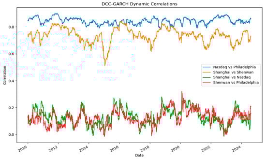
Figure 1.
DCC-GARCH dynamic correlations between the U.S. and China markets.
In contrast, cross-country correlations are notably weaker. The Shanghai–Nasdaq correlation fluctuates mostly between 0.10 and 0.30, with occasional spikes during major global events. This low baseline suggests limited short-term integration between the two countries’ broad markets, largely due to different macroeconomic drivers and regulatory environments. Similarly, the Shenwan–Philadelphia correlation exhibits a comparable low range of 0.10 to 0.30, despite the global supply chain connections between the semiconductor and electronics sectors. The correlation tends to rise during episodes of global disruption, such as supply chain shocks or rapid technological shifts, but remains modest on average. Event-specific patterns are evident across the sample period. During the 2008 financial crisis, correlations for both cross-country sectoral and broad-market pairings rose sharply, reflecting synchronized market stress. The 2018 U.S.–China trade conflict saw a decline in cross-country sectoral correlations, while the COVID-19 pandemic in 2020 produced a broad rebound in correlations, likely driven by global technology demand surges and supply chain constraints.
Overall, these findings indicate that while domestic market–sector linkages in both countries are strong, cross-country dependencies are weaker and more episodic, intensifying primarily during global crises. Because linear correlations—even when modeled dynamically—cannot distinguish between dependence in normal times and co-movements concentrated in the distribution tails, we next turn to a copula framework to characterize nonlinear and asymmetric tail dependence. In particular, Section 3.4 estimates Clayton, Gumbel, and t-copulas for the return series to identify whether downturns or upturns are more likely to occur jointly, laying the groundwork for the VaR-based tail analysis in Section 3.5.
3.4. Copula Analysis for Return Series
To complement the linear correlations and time-varying dependencies identified by the DCC-GARCH model (Figure 1), we employ copula functions to capture nonlinear and asymmetric dependence structures in the return series. Copulas allow for the separation of marginal distributions from the joint distribution, enabling a flexible characterization of dependencies, particularly in the tails. Following the methodology outlined in Section 2.3.4, we fit three copula families to each market pair: the Clayton Copula for lower-tail dependence, the Gumbel Copula for upper-tail dependence, and the t = Copula for symmetric, tail-neutral dependence. The copula parameters and tail dependence coefficients ( and ) are estimated using maximum likelihood methods, with model selection guided by the Akaike Information Criterion (AIC) and robustness confirmed via the goodness-of-fit (GoF) test. Table 4 reports the best-fitting copula family for each market pair, along with the estimated dependence parameters and tail dependence coefficients. Lower-tail dependence () captures the probability of joint large losses, while upper-tail dependence () captures the probability of joint large gains. For the t-Copula, the tail dependence is symmetric, meaning that and are equal, reflecting balanced co-movements in both extreme downturns and upturns. The GoF test results confirm that the chosen copulas provide a good fit to the data, ensuring that the dependence structures are robust and accurately reflect the risk transmission dynamics across the markets.
Table 4.
Copula estimation results for return series.
The results reveal distinct patterns: (1) Nasdaq–Shanghai: The t-Copula provides the best fit, with low symmetric dependence, confirming that broad market linkages between the U.S. and China are moderate and balanced across tails. (2) Philadelphia–Shenwan: The Clayton Copula dominates, showing stronger lower-tail dependence, suggesting that during severe downturns in the U.S. semiconductor market, the Chinese electronics market is more likely to experience simultaneous losses. (3) Nasdaq–Philadelphia: The Gumbel Copula fits best, indicating stronger upper-tail dependence, consistent with the close integration of the U.S. broad market and its technology sector during bullish periods. (4) Shanghai–Shenwan: The t-Copula again fits best, with moderate symmetric dependence, reflecting steady domestic linkages between China’s broad market and electronics sector.
These findings enrich the DCC-GARCH results by highlighting how dependence structures vary not only in magnitude over time but also in symmetry and tail concentration. In particular, the strong lower-tail dependence between Philadelphia and Shenwan underscores the vulnerability of cross-border industrial linkages to downside shocks in the semiconductor sector, whereas the Nasdaq–Philadelphia upper-tail dominance reflects the reinforcing nature of positive sentiment and technology-driven rallies within the U.S. market. Compared with the return series, the subsequent analysis of VaR series in Section 3.5 will directly focus on extreme risk scenarios, allowing us to assess whether the tail dependencies identified here persist or change when attention is restricted solely to high-loss events.
3.5. Value-at-Risk (VaR) Series and Copula Analysis
3.5.1. VaR Series Estimation and Characteristics
The 5% daily VaR series for each index is estimated using the GARCH(1,1)-Skewed-t model described in Section 2.3.5. The estimation results are reported in Table 5. The fitted parameters successfully capture both volatility clustering and the distributional asymmetry of financial returns. Notably, all four markets exhibit negative skewness parameters (λ), indicating a higher likelihood of extreme negative returns. The shape parameter η varies across markets, with Shanghai (η = 4.96) showing the heaviest tails, implying the highest probability of extreme risk events, while Shenwan (η = 8.66) is closest to a normal distribution, indicating relatively lower risk. The persistence parameter β1 is close to 0.9 for all markets, confirming the long memory property of volatility typical in financial markets.
Table 5.
Estimation results of the GARCH(1,1)-Skewed-t model.
The VaR series in Figure 2 reveals pronounced spikes during periods of significant market stress, particularly the 2015 Chinese stock market crash and the 2020 COVID-19 pandemic. Among the four indices, Philadelphia shows the most pronounced surge in VaR during 2020, suggesting heightened vulnerability in the U.S. semiconductor sector. In contrast, the Shanghai and Shenwan indices exhibited sharper increases during the 2015 turbulence, reflecting the domestic roots of that crisis. Nasdaq demonstrates relatively smoother but still evident fluctuations, highlighting its role as a global benchmark that amplifies systemic shocks. These dynamics suggest that technology-related equity markets, while globally interconnected, display heterogeneous sensitivities to crisis events. The asymmetric patterns—where Chinese indices are more exposed to domestic regulatory and liquidity shocks, while the U.S. semiconductor sector is disproportionately affected by global demand disruptions—underscore the importance of disentangling region- and sector-specific vulnerabilities. Such findings provide strong justification for employing copula-based approaches to capture tail dependencies, as simple correlation measures would fail to reveal these nonlinear crisis-driven linkages.
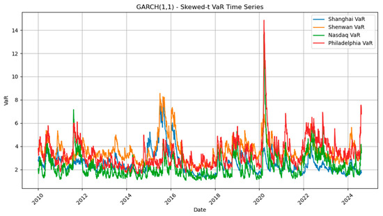
Figure 2.
VaR series from the GARCH(1,1)-Skewed-t model.
3.5.2. Copula Analysis for VaR Series
Given the strictly positive nature of the VaR series, the interpretation of tail dependence differs from that for return series: (1) Left tail—smaller VaR values (milder losses, market rebound). (2) Right tail—larger VaR values (extreme losses, market crash. In the copula framework: (1) Clayton copula (lower-tail dependence) measures co-movements during rebounds. (2) Gumbel copula (upper-tail dependence) captures co-movements during crashes. (3) Student-t copula models symmetric tail dependence for benchmark comparison.
We estimate copula parameters for four market pairs: Shanghai–Nasdaq, Shanghai–Shenwan, Nasdaq–Philadelphia, and Shenwan–Philadelphia. The best-fitting copula for each pair is selected using the Akaike Information Criterion (AIC), and tail dependence coefficients are computed to measure the probability of simultaneous extreme or mild loss events. Table 6 summarizes the results.
Table 6.
Copula estimation results for 5% VaR series.
The findings reveal distinct dependence structures: (1) Shanghai–Nasdaq: Stronger upper-tail dependence indicates that extreme losses in the U.S. broad market are more likely to coincide with extreme losses in China’s broad market, consistent with contagion effects during crises. (2) Shanghai–Shenwan: Symmetric dependence reflects the strong structural linkages within China’s markets, with similar reactions in both rebounds and downturns. (3) Nasdaq–Philadelphia: Highest upper-tail dependence among all pairs, confirming that U.S. sector-specific shocks are closely tied to overall market crashes. (4) Shenwan–Philadelphia: Higher lower-tail dependence suggests that recovery phases tend to be synchronized, likely due to demand rebounds in the global electronics supply chain.
Overall, the results indicate that extreme downside risk is more tightly integrated within U.S. markets and between U.S. and Chinese broad indices, while cross-border sectoral connections are stronger during milder loss phases.
3.6. Return Copula vs. VaR Copula Comparative Analysis
To highlight the added value of extending copula analysis from return series to Value-at-Risk (VaR) series, we compare the lower-tail and upper-tail dependence coefficients estimated in Section 3.4 and Section 3.5.2. The comparison allows us to assess how dependence structures shift when focusing on extreme risk events rather than average market conditions.
Figure 3 presents a side-by-side visualization of tail dependence coefficients for the four market pairs: Shanghai–Nasdaq, Shanghai–Shenwan, Nasdaq–Philadelphia, and Shenwan–Philadelphia, under both return-based and VaR-based copula models. Several patterns emerge from the comparison: (1) Amplification of Upper-Tail Dependence in VaR Copulas for Cross-Border Broad Market Pairs. For Shanghai–Nasdaq, the upper-tail dependence rises from 0.145 in returns to 0.31 in VaR series, indicating that joint extreme losses become more tightly linked when risk is measured in terms of potential losses rather than raw returns. (2) Persistence of Symmetric Dependence in Domestic Chinese Markets. The Shanghai–Shenwan pair shows similar dependence levels in both returns and VaR series , confirming that domestic linkages are stable across normal and stressed conditions. (3) Stronger Extreme Loss Linkages in U.S. Sectoral and Broad Market Pairings. For Nasdaq–Philadelphia, the upper-tail dependence increases markedly from 0.318 in returns to 0.42 in VaR series, reinforcing the finding that sector-specific shocks in the U.S. amplify during market crashes. (4) Shift Toward Lower-Tail Dependence in Cross-Border Sectoral Pairs. The Shenwan–Philadelphia pair changes from balanced or upper-tail dominance in returns to a pronounced lower-tail dominance in VaR series, suggesting that recovery phases are more synchronized than crashes in this pairing.
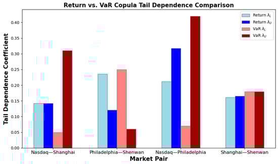
Figure 3.
Comparison of tail dependence coefficients between return and VaR copulas.
Overall, the comparative analysis confirms that VaR-based copula models sharpen the focus on extreme risk contagion and reveal patterns that are muted in return-based models. This distinction justifies the use of VaR copulas as a complementary tool for studying cross-market dependence, particularly for assessing systemic vulnerability under stress scenarios.
3.7. Dynamic Copula Analysis for VaR Series
To deepen our understanding of how extreme risk dependencies evolve over time, we estimate dynamic copula-based tail dependence for the 5% Value-at-Risk (VaR) series using a rolling window of 500 trading days with a step size of 100 days, as well as a robustness test with a 250-day window. Unlike static copula results, the dynamic approach highlights temporal shifts in risk linkages, especially during episodes of market stress.
Figure 4 displays the dynamic upper-tail dependence between the Shanghai Composite Index and the Nasdaq Composite Index. The time-varying fluctuates between 0.1 and 0.6, with an average close to the static estimate ( ≈ 0.31). Two distinct patterns emerge. First, during the pre-2015 period, upper-tail dependence remains relatively low and stable, consistent with limited contagion when global and domestic markets experienced moderate downturns. This suggests that under normal market conditions, the co-movement of extreme losses between the two indices was relatively weak, reflecting segmentation across national financial systems. Second, in the 2015–2016 and post-2020 periods, rises substantially, frequently peaking above 0.5. These surges coincide with the 2015 Chinese stock market crash—driven by domestic leverage and liquidity shocks—and the global COVID-19 shock in 2020, which triggered simultaneous stress across international markets. The pronounced spikes highlight that upper-tail dependence between U.S. and Chinese equity markets is not constant but episodic and event-driven, intensifying sharply during systemic crises. The robustness check with the 250-day window shows similar trends, further confirming the stability of the results.
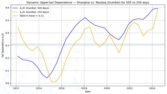
Figure 4.
Dynamic upper-tail dependence between Shanghai and Nasdaq (Gumbel copula ).
Figure 5 illustrates the dynamic lower-tail dependence between the Shenwan Electronics Index and the Philadelphia Semiconductor Index. The estimated values fluctuate between 0.0 and 0.7, with an average close to 0.25 as reported in Table 6, broadly consistent with the static estimates. Two notable phases can be identified. First, during the 2015–2016 period, there is a sharp surge in lower-tail dependence, with values approaching 0.6–0.7. This indicates highly synchronized rebound phases between the Chinese electronics sector and the U.S. semiconductor sector. Economically, this pattern can be attributed to the global demand recovery in technology supply chains following the 2015 Chinese market turbulence. The rebound was not isolated to domestic markets but rather spread across the semiconductor–electronics value chain, underscoring the extent to which these industries are globally integrated. Second, in the post-2018 period, moderates somewhat but remains persistently above pre-2015 levels. This stabilization at a higher baseline suggests that structural linkages between the two markets have deepened over time, especially as cross-border supply chains in semiconductors and electronics became increasingly interdependent. In particular, episodes of recovery following external shocks—such as trade tensions and pandemic disruptions—show that rebounds tend to be mutually reinforcing across the two sectors. The 250-day window analysis also reveals similar trends, supporting the robustness of the results.

Figure 5.
Dynamic lower-tail dependence between Shenwan and Philadelphia (Clayton copula ).
Overall, the dynamic pattern highlights that lower-tail dependence is not merely episodic but exhibits features of structural persistence. The results emphasize that synchronized rebounds are an inherent property of global technology markets, reflecting the intertwined nature of demand, production, and innovation in the electronics–semiconductor ecosystem. This has important implications for policymakers and investors alike: shocks to one side of the supply chain are likely to generate co-movements in the recovery phase across borders, limiting diversification opportunities and reinforcing systemic exposure to technology-cycle fluctuations.
4. Conclusions and Recommendation
4.1. Summary of Key Findings
This study systematically investigates the dependence structure between the U.S. and Chinese semiconductor–electronics markets by integrating linear correlation analysis, dynamic correlation modeling, and copula-based tail dependence estimation. Several key findings emerge:
(1) Static Dependence is Moderate but Statistically Significant. Kendall’s tau results reveal that within-country market–sector correlations are the strongest—Shanghai–Shenwan (0.312) in China and Nasdaq–Philadelphia (0.356) in the U.S.—reflecting strong domestic linkages between broad market conditions and sectoral performance. Cross-country correlations are weaker (e.g., Shanghai–Nasdaq: 0.149; Philadelphia–Shenwan: 0.224) but remain statistically significant, indicating the presence of systematic linkages despite structural and regulatory differences.
(2) Unidirectional Causality from U.S. to Chinese Markets. Granger causality tests consistently identify significant predictive power from U.S. broad and sectoral indices to their Chinese counterparts, while the reverse effect is absent. This asymmetry aligns with the global semiconductor–electronics value chain, where the U.S. dominates upstream innovation and market leadership.
(3) Dynamic Correlations are Stronger Domestically and Event-Driven Across Borders. DCC-GARCH results show persistently high domestic correlations (0.6–0.8 in China; ~0.8 in the U.S.), while cross-country correlations remain low (0.1–0.3) except during global crises, such as the 2008 financial crisis and the COVID-19 pandemic.
(4) Return Copula Analysis Reveals Tail Asymmetries. Lower-tail dependence dominates for Philadelphia–Shenwan, indicating vulnerability of the Chinese electronics sector to severe U.S. semiconductor downturns. Upper-tail dependence is stronger for Nasdaq–Philadelphia, reflecting synchronized gains during bullish U.S. market phases. Cross-country broad market linkages (Nasdaq–Shanghai) remain symmetric but modest in both tails.
(5) VaR Copula Analysis Highlights Extreme Risk Contagion. Using best-fitting copulas for each market pair (as reported in Table 6), we find that VaR-based measures amplify upper-tail dependence for cross-border broad market pairs (Shanghai–Nasdaq: rises from 0.145 in returns to 0.31 in VaR). Domestic Chinese linkages remain symmetric and stable across normal and stressed conditions. Within the U.S., sectoral and broad market pairs exhibit the strongest crash contagion (Nasdaq–Philadelphia: = 0.42), underscoring the concentration of systemic risk during downturns. By contrast, cross-border sectoral pairs (Shenwan–Philadelphia) show higher lower-tail dependence ( = 0.25), suggesting synchronized rebounds in the global electronics supply chain during recovery phases.
(6) Dynamic Copula Results Indicate Structural Rebound Linkages and Episodic Crash Contagion. Rolling-window analysis based on best-fitting copulas further refines these insights. For Shanghai–Nasdaq, Gumbel-based spikes during the 2015 Chinese equity crash and the 2020 COVID-19 pandemic, confirming that cross-border crash contagion is episodic and event-driven. For Shenwan–Philadelphia, Clayton-based displays a sustained upward trend since 2015, reflecting structurally embedded rebound linkages in technology supply chains. Taken together, these results underscore a dual-channel dependence structure: episodic contagion in downside risks and persistent co-movements in recovery phases.
Overall, the empirical evidence reveals a layered dependence structure: strong and persistent domestic linkages, asymmetric cross-border contagion patterns, and a dual nature of extreme dependence where downside risks are crisis-driven while rebound dynamics are structurally reinforced.
4.2. Policy Implications
The empirical results offer several policy-relevant insights for regulators, industry stakeholders, and investors in both China and the United States.
(1) Strengthening Systemic Risk Monitoring in Cross-Border Markets. The finding of episodic but significant upper-tail dependence in cross-country broad market pairs (e.g., Shanghai–Nasdaq) implies that systemic risk can transmit rapidly during global crises. Regulators should incorporate tail dependence indicators into macroprudential monitoring systems, particularly under Value-at-Risk (VaR) frameworks, to detect early warning signals of joint extreme losses. Cross-border regulatory coordination—such as information-sharing mechanisms between the China Securities Regulatory Commission (CSRC) and the U.S. Securities and Exchange Commission (SEC)—could enhance crisis-time responsiveness and reduce market fragmentation risks.
(2) Safeguarding Semiconductor–Electronics Industrial Security. The stronger lower-tail dependence between the U.S. semiconductor sector (Philadelphia) and the Chinese electronics sector (Shenwan) indicates heightened vulnerability of downstream Chinese firms to upstream shocks in U.S. technology markets. Industrial policy should emphasize supply chain resilience, including diversification of critical component sourcing and investment in indigenous chip fabrication technologies. Joint government–industry contingency planning for technology export controls, supply disruptions, and geopolitical shocks can mitigate cascading effects in both production and financial markets.
(3) Enhancing Capital Market Stability Through Domestic Linkages. The persistently high domestic correlations (Shanghai–Shenwan; Nasdaq–Philadelphia) suggest that sector-specific volatility can rapidly spill over to broader national markets. Domestic regulators should integrate sectoral stress testing into their financial stability frameworks, particularly for high-technology industries with concentrated market capitalization. Policies encouraging diversified sectoral investment within domestic markets—such as sector rotation funds or thematic ETFs—may help dilute concentrated exposure to technology sector shocks.
(4) Incorporating Tail-Asymmetry in Risk Management. The asymmetry between upper- and lower-tail dependencies across different market pairs highlights the need for scenario-based risk assessments. For example, portfolio stress tests should separately model crash-phase contagion (upper-tail in VaR) and rebound-phase synchronization (lower-tail in VaR), given their distinct drivers and implications. Derivatives market participants could design tail-hedging instruments tailored to asymmetric dependence patterns—such as structured options that provide greater protection against downside tail events in cross-border broad market positions.
(5) Long-Term Strategic Considerations. The structural strengthening of rebound dependencies since 2015 suggests an increasing integration of recovery cycles between the two countries. While this can foster co-movement in post-crisis growth phases, it also implies that macro policy synchronization (e.g., fiscal stimulus timing) could unintentionally amplify cross-border volatility. Coordinated communication of major policy actions could help smooth such effects.
In sum, the study underscores that extreme risk contagion is not constant but intensifies during global crises, and that tail dependence structures are asymmetric across market types. Policymakers should move beyond average correlation monitoring and adopt dynamic, tail-sensitive risk management approaches to safeguard both industrial security and financial stability in an increasingly interconnected global technology ecosystem.
4.3. Investment Strategies
The empirical findings provide actionable insights for global portfolio managers, hedge funds, and institutional investors seeking to optimize asset allocation and risk management in the semiconductor–electronics domain.
(1) Strategic Asset Allocation Based on Tail-Dependence Profiles. Cross-Border Broad Market Positions (Shanghai–Nasdaq): The amplification of upper-tail dependence in VaR-based analysis suggests that extreme downside risks in these markets tend to be synchronized during crises. For institutional investors and portfolio managers with large-scale assets, long-term exposure to both indices should be actively managed, potentially reducing simultaneous long exposure during early warning periods of systemic stress. For individual investors, particularly those with limited diversification options, it may be more practical to substitute one leg with defensive assets or consider ETFs that provide broad market exposure but with a defensive tilt.
(2) Domestic Market–Sector Positions (Shanghai–Shenwan; Nasdaq–Philadelphia). High and persistent domestic correlations imply that diversification benefits within national borders are limited. Institutional investors with larger portfolios should focus on cross-sector or cross-asset diversification (e.g., commodities, fixed income) rather than relying solely on domestic equity diversification. For individual investors, who may have more concentrated holdings, it is advisable to consider sectoral ETFs or mutual funds to balance risk across industries and reduce exposure to a single market or sector.
(3) Event-Driven Hedging Strategies. For U.S. sectoral–broad market pairs (Nasdaq–Philadelphia) with strong upper-tail dependence, crash-phase hedging can be implemented through protective puts or collar strategies on technology ETFs during periods of elevated volatility indices (VIX). For institutional investors, utilizing options on technology ETFs or hedging large positions through derivative instruments can help manage tail risk effectively. Individual investors can explore lower-cost hedging strategies such as exchange-traded put options or inverse ETFs, which provide a more accessible method to hedge portfolio risk during periods of high volatility. For China–U.S. sectoral pairs (Shenwan–Philadelphia) with stronger lower-tail dependence in VaR series, rebound-phase synchronization can be exploited through call spread strategies or long equity positions in both markets during early recovery phases, identified via macroeconomic or policy stimulus signals.
(4) Incorporating Dynamic Correlation in Tactical Allocation. The DCC-GARCH results highlight that cross-country correlations are episodic, spiking mainly during global shocks. Tactical allocation models should therefore be regime-switching in nature for institutional investors, adjusting exposure according to correlation regimes rather than static assumptions. Institutional investors may benefit from utilizing advanced risk models and machine learning-based signal extraction (e.g., regime classification using volatility, macro indicators, and policy news sentiment). For individual investors, simpler regime-switching strategies such as rebalancing portfolio exposure during periods of heightened market stress may be more practical. Machine learning and signal extraction could be used in personal investment strategies, but the focus should be on easier-to-implement tools such as volatility-based alerts or market trend-following strategies.
(5) Tail-Risk-Sensitive Portfolio Construction. The asymmetry between lower- and upper-tail dependencies underscores the value of tail-hedging overlays. For example: In markets with high upper-tail VaR dependence (Nasdaq–Philadelphia, Shanghai–Nasdaq), consider out-of-the-money put options or variance swaps as crash insurance. Institutional investors may allocate a portion of their portfolio to more sophisticated tail-risk hedges such as bespoke options or structured products, while individual investors can use more straightforward hedging tools like put options on ETFs or mutual funds that track these markets. In markets with pronounced lower-tail VaR dependence (Shenwan–Philadelphia), maintain dry powder capital to deploy during synchronized rebound opportunities. For institutional investors, this may involve maintaining cash reserves or liquid assets in anticipation of opportunities, while individual investors should ensure they have easy access to liquid funds in a similar manner.
(6) Long-Term Strategic Positioning in the Semiconductor–Electronics Value Chain. Given the vulnerability of Chinese downstream electronics to U.S. upstream semiconductor shocks, investors should monitor supply chain policy developments (e.g., export controls, subsidies) and adjust sector weights accordingly. Institutional investors may consider adjusting their exposure to semiconductor companies based on geopolitical risk assessments, potentially allocating capital to diversified global semiconductor ETFs or multinational firms with geographically diversified production to minimize specific geopolitical risks. Individual investors may prefer investing in semiconductor-focused ETFs or mutual funds that offer diversified exposure to the sector without the need to analyze individual stocks or geopolitical developments in detail.
In conclusion, the study’s findings support an adaptive, tail-aware, and event-sensitive investment framework, where allocation and hedging decisions are informed not only by average co-movements but also by the evolving structure of extreme dependencies between markets. Such a framework is particularly critical in technology-driven sectors that are both highly integrated globally and exposed to geopolitical uncertainty.
Author Contributions
Conceptualization, X.Z.; Methodology, X.Z. and H.L.; Formal Analysis, X.Z. and H.L.; Writing—Original Draft Preparation, H.L.; Writing—Review & Editing, X.Z. All authors have read and agreed to the published version of the manuscript.
Funding
This work was supported by the Key project of Zhejiang Provincial Natural Science Foundation [grant numbers LZ25G030002]; and the Humanities and Social Sciences Research Project of the Ministry of Education [grant number 19YJAZH056 & 25YJA790094].
Institutional Review Board Statement
Not applicable.
Informed Consent Statement
Not applicable.
Data Availability Statement
The data presented in this study are openly available in Wind database for China at https://www.wind.com.cn (accessed on 11 October 2024), and Yahoo Finance for the United States at https://finance.yahoo.com/ (accessed on 11 October 2024).
Conflicts of Interest
The authors declare no conflicts of interest.
References
- Akhtaruzzaman, M., Benkraiem, R., Boubaker, S., & Zopounidis, C. (2022). COVID-19 crisis and risk spillovers to developing economies: Evidence from Africa. Journal of International Development, 34(4), 898–918. [Google Scholar] [CrossRef] [PubMed]
- Akhtaruzzaman, M., Boubaker, S., & Sensoy, A. (2021). Financial contagion during COVID-19 crisis. Finance Research Letters, 38, 101604. [Google Scholar] [CrossRef] [PubMed]
- Allen, J. S. (2021). Do targeted trade sanctions against Chinese technology companies affect US firms? Evidence from an event study. Business and Politics, 23(3), 330–343. [Google Scholar] [CrossRef]
- Boako, G., Osei, K. A., & Agyekum, O. O. (2019). Analysing dynamic dependence between gold and stock returns: Evidence using stochastic and full-range tail dependence copula models. Finance Research Letters, 31, 105096. [Google Scholar] [CrossRef]
- Cherubini, U., Luciano, E., & Vecchiato, W. (2004). Copula methods in finance. John Wiley & Sons. [Google Scholar] [CrossRef]
- Clayton, D. G. (1978). A model for association in bivariate survival data. Biometrika, 65(1), 141–151. [Google Scholar] [CrossRef]
- Čeryová, B., & Árendáš, P. (2023). Vine copula approach to the intra-sectoral dependence analysis in the technology industry. Finance Research Letters, 54, 104889. [Google Scholar] [CrossRef]
- Du, J., Wang, S., & Li, Y. (2023). Analysis of stock markets risk spillover with copula models under the background of Chinese financial opening. International Journal of Finance & Economics, 28(4), 3997–4019. [Google Scholar] [CrossRef]
- Engle, R. (2002). Dynamic conditional correlation: A simple class of multivariate generalized autoregressive conditional heteroskedasticity models. Journal of Business & Economic Statistics, 20(3), 339–350. [Google Scholar] [CrossRef]
- Gubareva, M., & Strahl, S. (2023). Decoupling between the energy and semiconductor sectors during the pandemic: New evidence from wavelet analysis. Emerging Markets Finance and Trade, 59(6), 1707–1719. [Google Scholar] [CrossRef]
- Gumbel, E. J. (1960). Bivariate exponential distributions. Journal of the American Statistical Association, 55(292), 698–707. [Google Scholar] [CrossRef]
- Kinateder, H., Choudhury, T., Zaman, R., Scagnelli, S. D., & Sohel, N. (2021). Does boardroom gender diversity decrease credit risk in the financial sector? Worldwide evidence. Journal of International Financial Markets, Institutions and Money, 73, 101347. [Google Scholar] [CrossRef]
- Li, W., Lai, Y., Wang, C., & Tan, B. (2022). How do emerging debt market participants recognize firm internationalization? Evidence from effects on credit ratings. Emerging Markets Review, 54, 100939. [Google Scholar] [CrossRef]
- Liu, G., Long, W., Zhang, X., & Li, Q. (2019). Detecting financial data dependence structure by averaging mixture copulas. Econometric Theory, 35(4), 777–815. [Google Scholar] [CrossRef]
- Ng, S.-H., & Su, Y. (2025). Export response to technical barriers to trade: Evidence from high-tech exports of China to the United States. Journal of the Asia Pacific Economy, 30(3), 960–981. [Google Scholar] [CrossRef]
- Patton, A. J. (2006). Modelling asymmetric exchange rate dependence. International Economic Review, 47(2), 527–556. [Google Scholar] [CrossRef]
- Sklar, M. (1959). Fonctions de répartition à n dimensions et leurs marges. Annales de l’ISUP, 8(3), 229–231. [Google Scholar]
- Smith, J. (2024). Influence of digital transformation on firm performance in the service industry in the United States. International Journal of Business Strategies, 9(1), 63–74. [Google Scholar] [CrossRef]
- Tan, Y. (2024, September 23–25). Research on supply chain optimization strategy based on big data technology. 2024 International Conference on Electronics and Devices, Computational Science (ICEDCS) (pp. 384–390), Marseille, France. Available online: https://ieeexplore.ieee.org/document/10834965 (accessed on 8 December 2025).
- Xiong, W., Wu, D. D., & Yeung, J. H. Y. (2025). Semiconductor supply chain resilience and disruption: Insights, mitigation, and future directions. International Journal of Production Research, 63(9), 3442–3465. [Google Scholar] [CrossRef]
- Yousaf, I., Ali, S., & Wong, W. K. (2022). Return and volatility transmissions between metals and stocks: A study of the emerging Asian markets by using the VAR-AGARCH approach. Asia-Pacific Journal of Operational Research, 39(04), 2040020. [Google Scholar] [CrossRef]


Disclaimer/Publisher’s Note: The statements, opinions and data contained in all publications are solely those of the individual author(s) and contributor(s) and not of MDPI and/or the editor(s). MDPI and/or the editor(s) disclaim responsibility for any injury to people or property resulting from any ideas, methods, instructions or products referred to in the content. |
© 2025 by the authors. Licensee MDPI, Basel, Switzerland. This article is an open access article distributed under the terms and conditions of the Creative Commons Attribution (CC BY) license (https://creativecommons.org/licenses/by/4.0/).