Inverse DEA for Portfolio Volatility Targeting: Industry Evidence from Taiwan Stock Exchange

Abstract

This work develops an inverse data envelopment analysis (Inverse DEA) framework for portfolio optimization, treating return as a desirable output and volatility as an undesirable output. Using 20 industry-level portfolios from the Taiwan Stock Exchange (1365 stocks; FY-2020), we first evaluate efficiency with a directional-distance DEA model and identify 7 inefficient industries. We then formulate an Inverse DEA model that holds inputs and desirable outputs fixed and estimates the maximum feasible reduction in volatility. Estimated reductions range from 0.000827 to 0.007610, and substituting these targets into the base model drives each portfolio’s inefficiency score to zero $(\varphi =0)$, thereby making them efficient. To test robustness, we extend the analysis to a calm pre-crisis year (2019) and a recovery year (2021), which confirm that inefficiency and volatility-reduction targets behave logically across regimes, smaller cuts in stable markets, larger cuts in stressed conditions, and intermediate adjustments during recovery. We interpret these targets as theoretical envelopes that inform risk-reduction priorities rather than investable guarantees. The approach adds a forward-planning layer to DEA-based performance evaluation and provides portfolio managers with quantitative, regime-sensitive volatility-reduction targets at the industry level.

1. Introduction

Measuring and improving performance in finance increasingly requires tools that do more than rank decision-making units (DMUs); they must also translate diagnostics into actionable targets and insights. Data Envelopment Analysis (DEA) has long been used to benchmark banks, funds, exchanges, healthcare, energy companies, and stocks (Emrouznejad & Amin, 2023; Emrouznejad et al., 2023; Mergoni et al., 2024); however, standard DEA is essentially descriptive, as it evaluates current efficiency relative to an empirical production possibility set. When managers must set feasible improvement targets, for example, reducing risk (an undesirable output) or reallocating resources after a merger, standard DEA offers limited guidance. This is precisely where inverse DEA is valuable. Rather than asking “how efficient is a DMU given its data?”, Inverse DEA asks “how should a DMU’s inputs/outputs be adjusted to attain or preserve a desired efficiency level?” (T. Kehinde et al., 2023a).

Inverse DEA literature originates with Wei et al. (2000), who formalized the inverse problem: given a DMU’s efficiency relative to peers, how much additional output could it produce (or how much input must change) while maintaining that efficiency? That conceptual shift, turning DEA from a static scoreboard into a forward-planning instrument, sparked a stream of applications in banking, manufacturing, agriculture, healthcare, corporate restructuring, and, more recently, tourism management (Mergoni et al., 2024; Panwar et al., 2022).

In finance, Inverse DEA has been adopted where managers need targets under constraints: mergers and acquisitions (M&A), risk management, cost control, and multi-stage production systems (Amin & Oukil, 2019; Galagedera, 2024; Soltanifar et al., 2024; Wang et al., 2023; Yu et al., 2019). Early sectoral applications focused on banking, an industry rich with multiple inputs (labor, deposits, expenses) and outputs (interest income, services), and frequent restructuring (Amirteimoori & Allahviranloo, 2024; Gattoufi et al., 2014; Yu et al., 2019). For example, Gattoufi et al. (2014) pioneered Inverse DEA for bank mergers, deriving required input cuts and output levels for merged entities to hit specified efficiency targets, turning DEA from a passive assessor into a pre-merger planning tool. Later work generalized the idea: Amin et al. (2017b) introduced generalized Inverse DEA to model consolidation and split scenarios under predefined efficiency goals, while Amin et al. (2017a) distinguished minor and major consolidations depending on whether the merger shifts the frontier, an insight useful to managers and regulators concerned about market structure and competitiveness.

This evolving literature establishes Inverse DEA as a decision-support layer atop DEA: it provides attainable targets that respect the observed technology, the chosen returns-to-scale (RTS) assumption, and, in more recent models, managerial priorities, risk trade-offs, and dynamic or network structures. Yet, despite the breadth of applications of DEA in banking and M&A, capital markets and portfolio management remain comparatively underserved, particularly for setting risk targets (e.g., feasible reductions in return volatility) that keep relative efficiency unchanged. Classical methods, such as the mean–variance (M–V) approach (Markowitz, 1991) or risk-parity approaches, prescribe allocations but do not benchmark how much risk reduction is technologically feasible given peers’ performance. Standard DEA ranks funds or portfolios, but lacks a technique to translate a ranking into quantitative risk-reduction envelopes.

Against this backdrop, our study contributes a portfolio-oriented Inverse DEA framework that treats returns as desirable outputs and volatility as an undesirable output. Using a directional distance formulation, we estimate, for each inefficient portfolio/industry, the maximum feasible reduction in volatility that would place the unit on the efficient boundary (or preserve a specified efficiency level) without changing inputs or desirable outputs. In spirit, this mirrors the banking applications that target non-performing loans (undesirable) while holding revenue targets, but now tailored to capital markets, where the planning variable is risk itself. Methodologically, our approach is compatible with variable returns to scale and aligns with the literature that models undesirable outputs directly (An et al., 2019; Orisaremi et al., 2021; Yu et al., 2019) while maintaining the feasibility principles emphasized by Wei et al. (2000) and later Inverse DEA developments.

Our contributions are threefold. First, we develop a novel Inverse DEA framework for portfolio optimization that explicitly incorporates volatility as an undesirable output and estimates both feasible and maximum volatility-reduction targets for inefficient industry portfolios in the Taiwan Stock Exchange (TWSE). Second, we demonstrate through empirical analysis and validation that the proposed model provides actionable efficiency-improvement paths by showing how modest volatility reductions can transform underperforming portfolios into efficient ones. Third, we extend the Inverse DEA literature by situating our framework within recent methodological advances, including explicit handling of undesirable outputs and efficiency preservation, thereby offering a rigorous and reproducible approach to portfolio efficiency analysis.

The later sections of this article are detailed as follows: Section 2 provides an overview of prior research conducted within the relevant subject area. Section 3 illustrates the proposed framework in the context of inverse optimization. Section 4 of the paper discusses several aspects of data collection, model implementation, empirical analysis, and results. Finally, Section 5 presents a concise summary of the main findings, limitations, and potential opportunities for further investigation.

2. Literature Review

2.1. Portfolio Optimization Using DEA

Portfolio optimization is a cornerstone of asset allocation and remains central to decision-making by investors and portfolio managers (Trichilli et al., 2020). Traditionally, optimization has been framed by the mean–variance (M–V) paradigm of Markowitz (1991), which formalizes the trade-off between expected return and risk (Andria et al., 2017). In practice, however, a large body of work documents limitations of M–V and motivates complementary methods. Chief among these limitations are parameter-estimation error and solution sensitivity: small changes in estimated means or covariances can induce large swings in optimal weights, producing extreme and unstable portfolios (Bauder et al., 2021; Caldeira et al., 2023). Moreover, M–V relies exclusively on historical price data and offers no direct mechanism for incorporating managerial judgment or multi-criteria considerations beyond return and variance (Wijaya & Sidarto, 2023). These issues have spurred a search for approaches that preserve the spirit of risk–return optimization while being more robust to inputs and more expressive of investor preferences.

Within this broader agenda, diversification remains a foundational principle: combining imperfectly correlated assets reduces idiosyncratic risk without necessarily sacrificing return. Empirical work continues to find opportunities in specific settings to tackle this issue. For example, Oloko (2018) shows that U.S. and U.K. investors can achieve meaningful gains by adding Nigerian equities to their portfolios, illustrating that diversification benefits persist when exposures reach beyond developed markets. Institutional innovations also shape diversification potential. Pirgaip et al. (2021) analyze the South Eastern Europe Link (SEE Link), a platform connecting several regional exchanges, and find that, following its 2016 launch, return correlations and spillovers between the Zagreb and Bulgarian stock exchanges declined. This suggests that market-integration mechanisms can, paradoxically, create new diversification channels by expanding the investable set and improving liquidity across previously segmented markets. More broadly, both domestic and international diversification continue to be critical to portfolio selection (Yadav et al., 2023).

In parallel with diversification-based arguments, researchers have explored multi-criteria methods that move beyond the two-moment structure of M–V. DEA is one such nonparametric tool that evaluates relative performance using multiple inputs and outputs without imposing a specific functional form. Early evidence shows DEA’s promise for portfolio selection. In one of the first applications, Basso and Funari (2001) use DEA to select mutual funds in the Italian market and report performance improvements relative to conventional approaches. DEA’s appeal in this context is twofold. First, it naturally accommodates heterogeneous evaluation criteria, for instance, expense ratios, downside-risk measures, or liquidity, alongside return. Second, it produces peer-relative efficiency scores, highlighting best practices observed in the data and identifying feasible targets for improvement.

Beyond DEA, a rich multiple-criteria decision-making (MCDM) literature has emerged to handle complex ranking and selection problems (Andria et al., 2021), especially in equity markets. For example, Jing et al. (2023) apply six MCDM techniques: TOPSIS, Taxonomy, ARAS, VIKOR, COPRAS, and WASPAS, to 79 Tehran Stock Exchange firms using 15 financial indicators. They then aggregate the individual rankings via mean rank, Borda count, and Copeland procedures to identify robust stock selections under uncertainty. Such frameworks illustrate how multi-indicator evaluation can complement or precede optimization by narrowing the investable universe to alternatives that are attractive along several dimensions simultaneously.

Taken together, these strands, such as the recognition of M–V’s estimation fragility, the enduring logic of diversification, and the rise in multi-criteria evaluation, have shifted practice toward hybrid workflows. Investors first screen and rank assets with DEA or MCDM using broad information sets, then optimize over the shortlisted set, often with additional constraints to stabilize weights. This sequencing helps mitigate the pitfalls of pure M–V while retaining its intuitive appeal. It also creates a natural bridge to inverse and target-setting approaches (e.g., Inverse DEA), which do not merely assess current performance but quantify the feasible adjustments in inputs and outputs needed to attain or preserve efficiency. In subsequent sections, we build on this foundation, focusing on inverse DEA in finance, where undesirable outputs (e.g., volatility or risk) can be explicitly reduced while maintaining relative efficiency, thereby transforming benchmarking into forward-looking, implementable guidance for portfolio construction and risk control.

2.2. Selecting Inputs and Outputs for DEA in Equity Portfolio Poblem

Choosing the right inputs and outputs is crucial to the success of using DEA to solve the equity portfolio problem. The choice of these variables not only determines the accuracy and relevance of the analysis but also its discriminatory power. A generally applied rule of thumb for variable selection is that the quantity of indicator variables should be no greater than one-third of the quantity of DMUs (T. O. Kehinde et al., 2025b). To overcome this limitation, several methodologies have been put forth in scholarly works, outlined into two distinct classifications: the reduction in input and output quantities or the augmentation of the number of DMUs. The reduction in inputs and outputs can be achieved through the utilization of diverse criteria and methodologies, including expert views, statistical tests, principal component analysis, Shannon entropy, and other similar approaches. Risk has traditionally been perceived as a factor in production, representing the inherent uncertainties linked to investments. Tarnaud and Leleu (2018) suggested a paradigm shift using mathematical proofs, thus proposing a risk–return relationship as a terminal output of a financial production process that may be classified as desirable or undesirable. The basis of their argument is the concept that risk is not a factor that is intentionally incorporated into the production process but rather emerges as a result of the returns that are generated as outputs of production. Only a few works have embraced this novel classification in modeling their portfolios.

First, Kuo et al. (2021) evaluate the efficiency of 9 industry-based portfolios listed on the CSI-300 index. The authors followed the new classification paradigm that was proposed by Tarnaud and Leleu (2018), where financial ratios were used as inputs and technical ratios as outputs. The technical ratios serve as momentum indicators, duly represented as return and risk. The model under consideration utilizes approaches such as network DEA, AHP, and Second-Order Cone Programming (SOCP). However, their study did not employ inverse optimization techniques to determine the optimal changes required to improve the industry-based portfolios’ efficiency under consideration. In addition, the researchers used a reduced dataset exclusively comprising 140 equities from China’s CSI-300 index.

Second, Zeng et al. (2022) adopted the same novel paradigm of return–risk classification proposed by Tarnaud and Leleu (2018) to modify the energy mix by employing DEA and portfolio theory. The authors suggest that optimizing an energy mix can enhance resource utilization and diminish environmental impact. This was new since past research has failed to offer practical recommendations for adjusting the energy mix in this viable manner. In order to address this flaw, the authors commence by analyzing the return and risk associated with various energy technologies, subsequently formulating an energy portfolio. Later, a DEA model is constructed to assess the energy efficiency and optimize the energy composition. Ultimately, the researchers implement their methodology within the Chinese power sector, demonstrating the potential for substantial increases in the share of renewable energy sources and considerable reductions in carbon emissions through adjusting the energy mix.

Unlike the last two cited studies, Ebrahimi et al. (2021) developed a novel non-linear programming and non-radial DEA approach to selecting and evaluating financial asset portfolios. The output variables under consideration are the mean return and the variance of returns, with the latter being seen as undesirable. The authors propose a novel efficiency measure that includes good and bad outputs, as well as non-radial and slack-based attributes. The researchers implement their methodology on a subset of 11 banks and credit institutions that are publicly traded on the Tehran Stock Exchange. Subsequently, they classify and order these entities based on their respective efficiency scores.

To the best of our knowledge, no work has applied Inverse DEA in portfolio optimization. Our research provides a novel approach to portfolio optimization by integrating financial ratios and momentum indications, as well as revising the concept of risk. This perspective allows for more refined and comprehensive assessments.

2.3. Inverse DEA in Finance

Inverse DEA has evolved in finance as a target-setting complement to standard DEA, enabling managers to determine how inputs or outputs must change to attain or preserve efficiency. Early banking applications show how Inverse DEA can be embedded in richer benchmarking contexts. For example, Hosseinzadeh Lotfi et al. (2012) integrate Inverse DEA with context-dependent frontiers, allowing branch managers to forecast output requirements not only relative to the global best practice but also vis-à-vis progressively stronger peer sets. In corporate restructuring, Gattoufi et al. (2014) pioneer Inverse DEA for bank mergers, deriving pre-merger targets for the merged entity’s inputs and outputs consistent with a chosen efficiency level and thereby turning efficiency analysis into actionable M&A planning. On data realism, Amin and Al-Muharrami (2018) and Ghiyasi and Zhu (2020) accommodate negative data (e.g., losses) under SORM/VRS settings, and Soltanifar et al. (2025) extend Inverse DEA to ratio data, a common format for financial indicators. Regarding preferences, Soleimani-Chamkhorami et al. (2019) preserve cost and revenue efficiency when data change; Amin et al. (2019) embed goal programming to prioritize resources during mergers; and Soltanifar et al. (2024) propose a common-set-of-weights Inverse DEA to analyze multiple merger scenarios consistently.

A second strand models risk and multi-stage technologies explicitly. With undesirable outputs, banking studies set feasible risk-reduction or cost-containment targets: Yu et al. (2019) link efficiency with credit risk, while An et al. (2019) build a two-stage Inverse DEA including non-performing loans. Extending beyond “black-box” models, Amin and Ibn-Boamah (2021) use two-stage Inverse DEA to quantify merger gains across intermediate and final outputs. Collectively, these contributions reposition Inverse DEA from a diagnostic add-on to a decision-support engine: it sets feasible, efficiency-consistent targets for mergers, alliances, risk reduction, and resource planning across static, networked, and dynamic technologies, under realistic data constraints and managerial priorities. Table 1 provides a summary of notable works on inverse DEA in finance.

Table 1. Overview of recent studies on Inverse DEA in finance.

Author(s)	Method	Application(s)
Ghiyasi and Zhu (2020)	Inverse DEA under VRS with mixed-sign (negative) data via SORM	Banking
Soleimani-Chamkhorami et al. (2020)	Ranks efficient DMUs by required input increments at fixed efficiency	Banking
Zeinodin and Ghobadi (2020)	Dynamic Inverse DEA for mergers with inter-temporal carryovers	Banking, M&A
Guijarro et al. (2020)	Inverse DEA + genetic algorithms for sector-wide restructuring with global efficiency target and merger cardinality limits.	Banking, higher education
Ghobadi (2021)	Inverse DEA for mergers with interval (uncertain) data; estimates inherited inputs/outputs and achievable efficiency bounds.	Banking, M&A
Daryani et al. (2021)	Two-stage Inverse DEA with price/cost data	Banking/supply chains
Ghomi et al. (2021)	Stochastic Inverse DEA with (weak) Pareto at level α	Banking
Amin and Ibn-Boamah (2021)	Two-stage Inverse DEA for bank mergers	Banking, M&A
Soltanifar et al. (2023)	Inverse DEA-R handling negative ratios	Banking, M&A
Asadi et al. (2023)	Inverse FDH (non-convex) with double frontiers	Banking
Ghobadi et al. (2023)	Dynamic Inverse DEA estimating inputs/outputs	Banking, time-dependent planning
Amin and Ibn-Boamah (2023)	DEA + Inverse DEA for partnerships; redistributes inputs/outputs; alliances boost competitiveness.	Banking, strategic alliances
Gerami et al. (2023)	Generalized Inverse DEA with value efficiency	Banking, mergers/splits
Sohrabi et al. (2024)	DEA-R + Inverse DEA-R for alliances	Banking, alliances
Ibn-Boamah and Amin (2024)	Inverse DEA for partner selection in mergers	Banking, alliances
Ghiyasi (2024)	New Inverse DEA for time substitution	Economic planning
Soltanifar et al. (2024)	CSW-Inverse DEA for mergers; analyzes multiple scenarios simultaneously.	Banking
Amirteimoori and Allahviranloo (2024)	Statistical Inverse DEA corrector for efficient DMUs	Banking
Ghiyasi (2025)	Defines consolidation types (minor/major) using pre/post effects	Banking, M&A
Ghiyasi and Zhu (2025)	Parallel Inverse DEA with/without price info	Banking
Soltanifar et al. (2025)	Inverse DEA-R for ratio data with negatives	Healthcare, finance
Akbarian and Oukil (2025)	Inverse non-radial ERM for ratios	Finance
T. O. Kehinde et al. (2025b)	SET–DEA–IDEA for stock ranking	Stock market

2.4. Research Gap

Despite rapid advances that position Inverse DEA as a prescriptive, efficiency-consistent target-setting tool in finance, the literature remains concentrated in intermediation settings, bank branches, mergers, alliances, and multi-stage banking technologies, often with extensions for negative/ratio data, goal preferences, and uncertainty. What is largely missing is a capital-markets application like stock markets, which is highly volatile (T. Kehinde et al., 2023b, 2023c), where Inverse DEA can be used to generate actionable, frontier-consistent risk targets for equity portfolios, where return is a desirable output and volatility is explicitly modeled as an undesirable output within a directional-distance framework. Existing studies do not provide an Inverse DEA blueprint for portfolio optimization. Also, existing studies do not combine fundamental liquidity/asset-use/leverage ratios with return–volatility outputs to diagnose inefficiency, and do not supply implementable volatility-reduction paths (minimum vs. maximum feasible cuts) that can be embedded in risk budgets and governance. Moreover, prior work rarely examines Inverse DEA under a stress-period production set to derive crisis-robust prescriptions, nor does it articulate a transparent “net-zero volatility” bound as a technology-based limit rather than a trading claim. Our study fills this gap by unifying directional distance DEA diagnostics with an Inverse DEA planner for TWSE industry portfolios, delivering theoretically feasible volatility cuts at current returns, ranking sectors by residual risk for prioritization, and demonstrating ex-post feasibility (frontier attainment) once the inverse targets are applied.

3. Methodology

This section presents the methodological framework used to extend Inverse DEA to portfolio volatility targeting. We proceed in a sequence: first introducing the base model for efficiency evaluation, then the Inverse DEA formulation, followed by our proposed model tailored for volatility reduction in stock portfolios. To ensure clarity, we begin with the notation.

Indices and sets

n: total number of DMUs

k: target DMU being evaluated (k = 1, 2, …, n)

j: index for the DMU under evaluation (j = 1, 2, …, n)

i: index for input

r: index of good output

Parameters

$x_{ij}$: input for DMUj (j = 1, 2, …, n)

$y_{rj}^g$: good output (Return) for DMUj (j = 1, 2, …, n)

$y_{pj}^b$: bad output (Risk) for DMUj (j = 1, 2, …, n)

Decision variables

${\psi }_k$: efficiency score of DMUk under evaluation

${\varphi }_k$: inefficiency score of DMUk under evaluation

${\lambda }_j$: weight assigned to DMUj (j = 1, 2, …, n)

3.1. Model Formulation

Step 1: The first stage applies the base model, Directional Distance Function (DDF) DEA model (Chung et al., 1997; Orisaremi et al., 2021; Wegener & Amin, 2019), which incorporates both desirable and undesirable outputs. Efficiency is measured by the extent to which a DMU can increase desirable outputs while minimizing undesirable outputs and inputs. The base model (M1) helps estimate the inefficiency score $(\varphi )$ in individual portfolios for any $DM{U}_k\forall k=1,\dots ,n$.

$$\begin{array}{l}{\varphi }_k^{*}=\max {\varphi }_k\\ s.t.\\ {\displaystyle \sum _{j=1}^n{\lambda }_j{x}_{ij}\le x_{ik} where i=1,\dots ,m}\\ {\displaystyle \sum _{j=1}^n{\lambda }_j{y}_{rj}^g\ge (1+\varphi )y_{rk}^g where\mathrm{r}=1,\dots ,s}\\ {\displaystyle \sum _{j=1}^n{\lambda }_j{y}_{pj}^b=(1-\varphi )y_{pk}^b where\mathrm{p}=1,\dots ,q}\\ {\displaystyle \sum _{j=1}^n{\lambda }_j=1}\\ {\lambda }_j\ge 0 where j=1,\dots ,n\end{array}$$

(M1)

The inefficiency score, ${\varphi }_j$, for $DM{U}_j$ is expressed as:

$${\varphi }_j=\left\{\begin{array}{l}>0,{\mathrm{if}\mathrm{DMU}}_j\mathrm{is}\mathrm{efficient}\\ =0,{\mathrm{if}\mathrm{DMU}}_j\mathrm{is}\mathrm{inefficient}\end{array}\right.$$

(1)

Thus:

• ${\varphi }_j=0$, implies efficiency (efficiency score = 1).
• ${\varphi }_j>0$, implies inefficiency.

Note: Here, ${\lambda }_j$ denotes the DEA intensity (reference) weights that generate a convex combination of peer DMUs under VRS to define the benchmarking frontier and projections; these do not correspond to asset-allocation weights in a tradeable portfolio.

The relationship between inefficiency, $\varphi$, and efficiency, $\psi$, is expressed as:

$${\psi }_k={\displaystyle \frac{(1-{\varphi }_k^{*})}{(1+{\varphi }_k^{*})}}$$

(2)

While each industry-level portfolio is modeled as a DMU. A DMU is deemed efficient in the DEA sense if no other observed portfolio can generate equal or higher return with lower volatility and comparable inputs. The inclusion of both return (as a desirable output) and volatility (as an undesirable output) aligns directly with our proposed framework. This structure is consistent with our research aim: “How much must volatility be reduced to make a portfolio efficient, without altering its return or input profile?” By modeling good and bad outputs separately, the framework preserves the financial–production perspective and allows the inverse optimization to generate frontier-consistent volatility reduction targets.

The efficiency measure is peer-relative and nonparametric, relying solely on the observed production possibility set. By contrast, in traditional mean–variance (M–V) portfolio theory, efficiency is defined in terms of the global return–risk frontier: a portfolio is efficient if no alternative allocation offers higher expected return for the same risk or lower risk for the same return, given the estimated covariance matrix. While both approaches share the principle of identifying “nondominated” portfolios, DEA efficiency is data-driven and benchmarking-based, whereas M–V is model-based and distribution-dependent. Our framework applies the former definition, which evaluates efficiency relative to industry peers without requiring distributional assumptions.

Step 2: By formulating the inverse problem of M1, which takes the form of a multi-objective linear program (MOLP), Wegener and Amin (2019) proposed model M2. M2 interprets input fluctuations as propagating through to both good and bad outputs, and it explicitly sets up an optimization that minimizes the variations on bad outputs while still achieving efficiency.

Let ${\alpha }_{ik}$ denote the fluctuation in the $i^{th}$ input, which leads to a corresponding change ${\beta }_{rk}$ in the $r^{th}$ good output, accompanied by a modification ${\gamma }_{pk}$ in the $p^{th}$ bad output. The intent is to minimize the variations in all the undesired outputs. The model M2, which serves as the inverse optimization approach of the problem, is expressed as follows:

$$\begin{array}{l}\min \gamma =({\gamma }_{11},\dots ,{\gamma }_{q1},\dots ,{\gamma }_{1t},\dots ,{\gamma }_{qt})\\ s.t.\\ {\displaystyle \sum _{j\in A}{\lambda }_j^k}{x}_{ij}+{\displaystyle \sum _{l\in B}{\overline{\lambda }}_l^k({\alpha }_{il}+x_{il})}-({\alpha }_{ik}+x_{ik})\le 0\\ \forall k\in S,i=1,\dots ,m\\ {\displaystyle \sum _{j\in A}{\lambda }_j^k}{y}_{rj}^g+{\displaystyle \sum _{l\in B}{\overline{\lambda }}_l^k({\beta }_{rl}+y_{rl}^g)}-(1+{\overline{\varphi }}_k)\mathrm{x}({\beta }_{rk}+y_{rk}^g)\ge 0\\ \forall k\in S,r=1,\dots ,s\\ {\displaystyle \sum _{j\in A}{\lambda }_j^k}{y}_{pj}^b+{\displaystyle \sum _{l\in B}{\overline{\lambda }}_l^k({\gamma }_{pl}+y_{pl}^b)}-(1-{\overline{\varphi }}_k)\mathrm{x}({\gamma }_{pk}+y_{pk}^b)=0\\ \forall k\in S,p=1,\dots ,q\\ {\displaystyle \sum _{j\in A}{\lambda }_j^k}+{\displaystyle \sum _{l\in B}{\overline{\lambda }}_l^k=1 \forall k\in S}\\ {\displaystyle \sum _{k\in S}{\beta }_{rk}}={\overline{y}}_r^g r=1,\dots ,s\\ \hspace{1em}{\alpha }_{ik}\ge 0, {\beta }_{rk}\ge 0, {\gamma }_{pk}\ge 0 \forall k\in S, i=1,\dots ,m\\ \hspace{1em}{\lambda }_j^k\ge 0, {\overline{\lambda }}_l^k\ge 0, \forall k,l\in B, \forall j\in A\end{array}$$

(M2)

Step 3: Building on model M2, model M3 streamlines the inverse DEA formulation by restricting the reference set exclusively to efficient peers identified in M1. This modification ensures that inefficient portfolios are benchmarked only against empirically efficient frontiers, avoiding distortions caused by referencing other inefficient units. The result is a more realistic adjustment pathway toward efficiency. The original portfolio set can be dichotomized into subsets A and B. Subset A aggregates portfolios deemed efficient, while subset B collates the inefficient ones. Importantly, it is worth noting that within subset A, weights of efficient units are assigned ${\lambda }_j^k\ge 0,\forall j\in A$. Conversely, units in subset B are assigned weights ${\overline{\lambda }}_l^k\ge 0,\forall l\in B$. To preserve the intrinsic ${\varphi }_k^{*}$ of DMUs post-output production, decision-makers are guided to ensure ${\overline{\varphi }}_k\le {\varphi }_k^{*}$ (typically setting all values of ${\overline{\varphi }}_k$ at 3 d.p. equivalent of ${\varphi }_k^{*}$ without rounding up) within the application framework. By simplification, model (M2) approach produced a streamlined model, termed model M3.

$$\begin{array}{l}\min \gamma =({\gamma }_1+{\gamma }_2+,\dots ,+{\gamma }_t)\\ s.t.\\ {\displaystyle \sum _{j\in A}{\lambda }_j^k}{x}_{ij}\le ({\alpha }_{ik}+x_{ik}) \forall k\in S,\\ {\displaystyle \sum _{j\in A}{\lambda }_j^k}{y}_{rj}^g\ge (1+{\overline{\varphi }}_k)\mathrm{x}({\beta }_{rk}+y_{rk}^g) \forall k\in S,\\ {\displaystyle \sum _{j\in A}{\lambda }_j^k}{y}_{pj}^b=(1-{\overline{\varphi }}_k)\mathrm{x}({\gamma }_{pk}+y_{pk}^b) \forall k\in S,\\ {\displaystyle \sum _{j\in A}{\lambda }_j^k}=1 \forall k\in S\\ {\displaystyle \sum _{k\in S}{\beta }_{rk}}={\overline{y}}_r^g\\ {\alpha }_{ik}\ge 0, {\beta }_{rk}\ge 0, {\gamma }_{pk}\ge 0 \forall k\in S,\\ {\lambda }_j^k\ge 0, {\overline{\lambda }}_l^k\ge 0,\forall k,l\in B,\forall j\in A\end{array}$$

(M3)

While model M3 offers a practical framework for managing undesirable outputs, a significant limitation constrains its practical application. Specifically, the model necessitates an increase in both desirable and undesirable outputs as a prerequisite for any subsequent reduction in the latter. The present study aims to overcome this constraint by developing a novel model specifically designed to enable the direct decrease in undesirable outputs.

Step 4 (Proposed model): Recognizing that portfolio managers primarily seek to reduce volatility rather than alter inputs or sacrifice returns, model M4 specializes the inverse framework. Here, inputs and desirable outputs are fixed, and the only decision variable is the reduction in volatility. By maximizing the feasible reduction in σ while maintaining the original return, R, M4 provides a targeted strategy for transforming inefficient portfolios without altering their investment profile.

The central problem addressed is the quantification of the necessary volatility reduction for an inefficient portfolio to reach the efficient frontier, conditional on existing input levels and the current state of financial production technology. To handle this, we assumed all the variations in the desirable output and inputs are equal to zero. This simply means that, in the present financial production process, the values ${\beta }_{rk}={\alpha }_{ik}$ must be equal to zero. The anticipated decrease in volatility suggests that ${\gamma }_{pk}$ must exhibit a reduction from its current level. This pursuit of net-zero-risk portfolios necessitates a new objective: maximizing the decrease in volatility for each inefficient portfolio. Since volatility is the sole undesirable output in our framework, indexed as $p=1$, maximizing its reduction becomes the primary mechanism for improving efficiency. A greater reduction in volatility corresponds to a closer alignment with the efficient frontier. Integrating these principles leads to the formulation of model M4.

$$\begin{array}{l}\max \gamma =({\gamma }_1+{\gamma }_2+,\dots ,+{\gamma }_t)\\ s.t.\\ {\displaystyle \sum _{j\in A}{\lambda }_j^k}{x}_{ij}\le x_{ik} \forall k\in S,i=1,\dots ,m\\ {\displaystyle \sum _{j\in A}{\lambda }_j^k}{y}_{rj}^g\ge (1+{\overline{\varphi }}_k)\mathrm{x}{y}_{rk}^g \forall k\in S,r=1,\dots ,s\\ {\displaystyle \sum _{j\in A}{\lambda }_j^k}{y}_{pj}^b=(1-{\overline{\varphi }}_k)\mathrm{x}(y_{pk}^b-{\gamma }_{pk}) \forall k\in S,p=1,\dots ,q\\ {\displaystyle \sum _{j\in A}{\lambda }_j^k}=1 \forall k\in S\\ {\gamma }_{pk}\le y_{pk}^b\\ {\overline{\theta }}_k\ge 0, {\gamma }_{pk}\ge 0 \forall k\in S, i=1,\dots ,m\\ {\lambda }_j^k\ge 0, \forall k,l\in B, \forall j\in A\end{array}$$

(M4)

Step 5: Finally, model M5 operationalizes model M4 at the individual DMU level. For each inefficient portfolio, the model computes both the potential volatility reduction (attainable with a slightly stricter efficiency target, truncated to three decimals) and the maximum volatility reduction (corresponding to the theoretical boundary where inefficiency is eliminated). This step delivers actionable estimates of volatility decreases and validates them by re-running model (M1) with updated values to confirm that inefficiency scores collapse to zero.

$$\begin{array}{l}\max {\gamma }^{*}={\gamma }_{pk}\\ s.t.\\ {\displaystyle \sum _{j\in A}{\lambda }_j^k}{x}_{ij}\le x_{ik} i=1,\dots ,m\\ {\displaystyle \sum _{j\in A}{\lambda }_j^k}{y}_{rj}^g\ge (1+{\overline{\varphi }}_k)\mathrm{x}{y}_{rk}^g r=1,\dots ,s\\ {\displaystyle \sum _{j\in A}{\lambda }_j^k}{y}_{pj}^b=(1-{\overline{\varphi }}_k)\mathrm{x}(y_{pk}^b-{\gamma }_{pk}) p=1,\dots ,q\\ {\displaystyle \sum _{j\in A}{\lambda }_j^k}=1\\ {\gamma }_{pk}\le y_{pk}^b\\ {\gamma }_{pk}\ge 0\\ {\lambda }_j^k\ge 0,\forall l\in B,\forall j\in A\end{array}$$

(M5)

Model M5 yields feasible volatility-reduction targets at fixed inputs and return; these targets guide post-processing allocation rather than directly determining investable weights. It introduces an Inverse DEA model tailored to evaluate potential volatility reductions. Using the value of ${\varphi }_k^{*}$ derived from model (M1), we strategically determine ${\overline{\varphi }}_k$ to ensure its value aligns with specific criteria. Crucially, we establish that ${\overline{\varphi }}_k$ is slightly below ${\varphi }_k^{*}$, that is, ${\overline{\varphi }}_k\le {\varphi }_k^{*}$ expressed in three decimal points without rounding up. The parameter ${\gamma }^{*}$ in model M5 stands for the least possible decrease in volatility, represented as ${\gamma }_{pk}^{\min }$. This numeric becomes pivotal in achieving one of our goals. When a value of ${\gamma }^{*}=0$, it indicates the existing volatility is at its lowest point, making further reductions infeasible. A discernible link materializes between the variable ${\gamma }^{*}$ and the estimated parameter ${\overline{\varphi }}_k$, leading to the formulation of a specific proposition and its subsequent validation. All optimization models were solved using the LINGO 20 software package.

Theorem 1.

This optimal state emerges precisely when the projected value of ${\overline{\varphi }}_k=0$, leading to the condition $y_{pk}^b={\gamma }_{pk}^{\max }$.

Proof. 

In model (M5), set A encompasses a group of DMUs that are efficient, having delineated the efficiency frontier in model (M1) and thereby necessitating no further enhancement. □

Thus, the constraints ${\displaystyle \sum _{j\in A}{\lambda }_j^k}{y}_{rj}^g$, and ${\displaystyle \sum _{j\in A}{\lambda }_j^k}{y}_{pj}^b$ in model (M5) apply to the DMUs that are efficient while $(1+{\overline{\varphi }}_k)\mathrm{x}{y}_{rk}^g$, and $(1-{\overline{\varphi }}_k)\mathrm{x}(y_{pk}^b-{\gamma }_{pk})$ applies to inefficient $DM{U}_k$. This proof is articulated through Equations (3)–(5).

$$(1-{\overline{\varphi }}_k)\mathrm{x}(y_{pk}^b-{\gamma }_{pk})=0$$

(3)

$$\mathrm{At}{\overline{\varphi }}_k=0,y_{pk}^b-{\gamma }_{pk}=0$$

(4)

$$y_{pk}^b={\gamma }_{pk}={\gamma }_{pk}^{\max }$$

(5)

Empirical validation of this theorem will be provided through a numerical test in a subsequent section. This result directly fulfills one of the central objectives of this research.

3.2. Net Zero Volatility (NZV) Goal

Equity investing inevitably entails risk; even “safe” instruments (e.g., government bills) exhibit variability due to inflation and interest-rate uncertainty. Our contribution is not to claim the existence of a riskless stock portfolio, but to formalize a theoretical boundary case, the NZV target, within the Inverse DEA framework. This target is defined relative to the production technology estimated from the data and the directional distance setup used in model (M1). It serves as a stress-test style benchmark: how much of the observed volatility could in principle be eliminated, holding inputs and desirable outputs fixed, before the portfolio becomes DEA-efficient?

Definition 1.

Model M5 pinpoints the juncture of optimal reduction in volatility (bad output).

$$y_{pk}^{\max }\mathrm{only}\mathrm{occurs}\mathrm{when}{\overline{\varphi }}_k=0$$

Definition 2.

The feasibility of a net zero portfolio volatility centers on the scenario where $y_{pk}^b={\gamma }_{pk}^{\max }$.

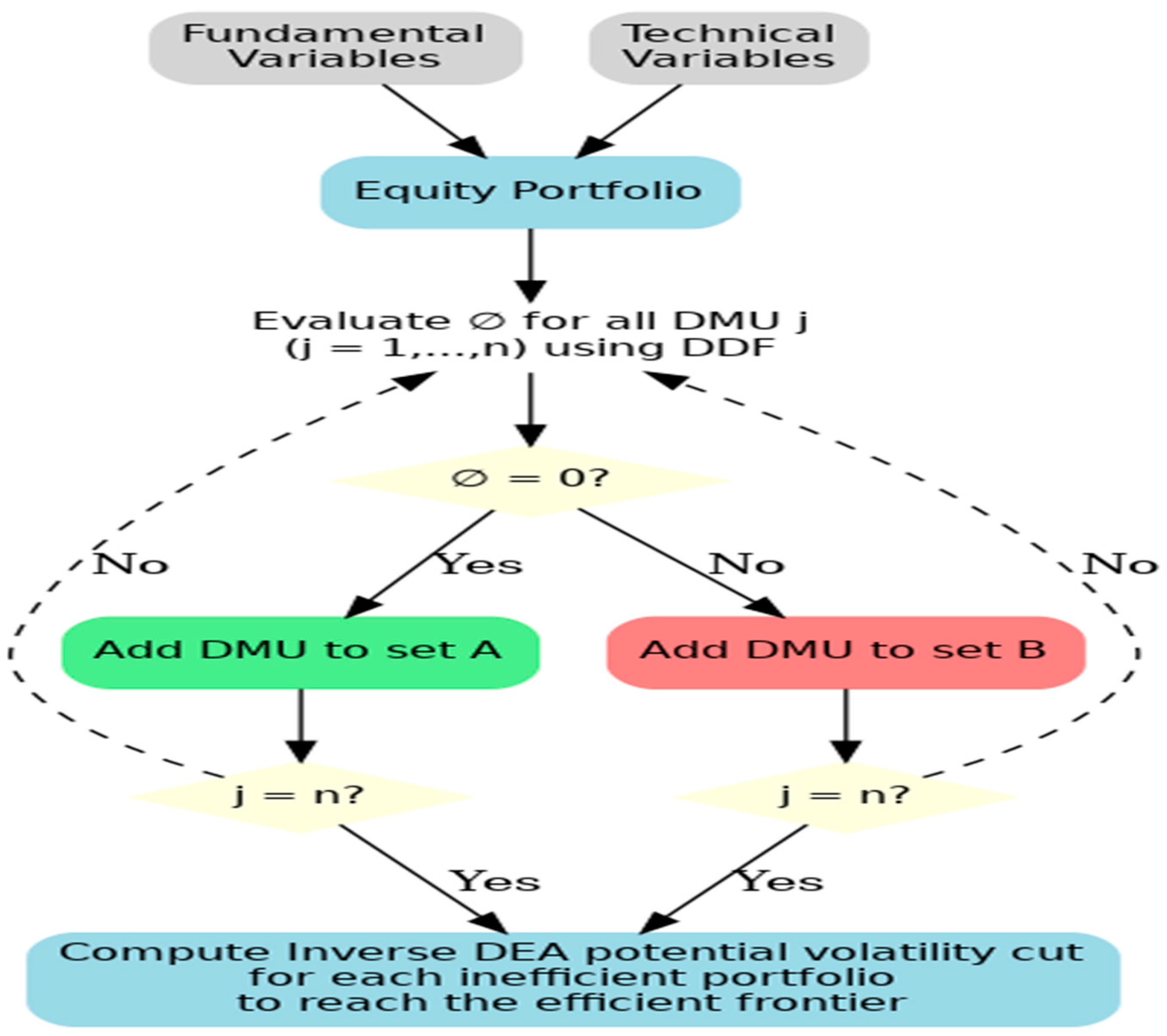
These definitions formalize the NZV goal, which is achieved when the maximum feasible reduction in volatility equals its current value, leaving no residual volatility. This process is illustrated in Figure 1, which outlines the methodological framework. The initial step involves calculating the inefficiency score for each DMU.

Figure 1. Framework for NZV goal.

The process commences with the evaluation of the inefficiency score for every DMU. Portfolios are deemed efficient and sorted into subset A if their ${\varphi }_k^{*}=0$. Conversely, portfolios are grouped into subset B if found to be inefficient, that is, their ${\varphi }_k^{*}>0$. For any inefficient portfolio, the utmost reduction in volatility, symbolized as ${\gamma }^{\max }$ is reached when the target ${\overline{\varphi }}_k=0$, thus nullifying its $\varphi$ score. If the deduced maximum reduction mirrors the actual volatility value, it implies no divergence, suggesting a NZV portfolio for any inefficient portfolio to become efficient.

4. Empirical Analysis and Discussion

4.1. Data Source and Statistics

We focus on the TWSE for three strategic reasons. First, Taiwan operates a mature, rules-based market with high disclosure quality; TWSE ranked eighth in Asia and seventeenth worldwide by market capitalization in 2023 (Statista, 2023). Second, Taiwan is a pivotal node in global technology supply chains, especially semiconductors and electronics, whose outputs surged with the post-pandemic digitalization wave; in 2021, the semiconductor industry’s output value reached about USD 145.8 billion, underscoring Taiwan’s global dominance (Zhou, 2023). Third, the COVID-19 period provides a natural stress test for portfolio efficiency and risk management, allowing us to examine inverse DEA targets under a pronounced macro–financial shock.

Firm-level data come from the Taiwan Economic Journal (TEJ) for fiscal year 2020 and cover fundamentals and market (price/momentum) information. The initial collection includes 1365 listed firms across 20 industries on TWSE: Automobile (AU, 31), Biotech and Medical (BM, 121), Building Material (BU, 78), Chemical (CH, 41), Communication and Internet (CI, 86), Computer and Peripherals (CP, 109), Cultural and Creative (CC, 25), Electronic Parts and Components (EC, 198), Electronic Products Distribution (EP, 33), Electric and Machinery (EM, 91), Foods (FO, 28), Information Service (IF, 35), Iron and Steel (IS, 45), Optoelectronic (OE, 113), Plastics (PL, 25), Semiconductor (SC, 151), Shipping and Transportation (ST, 28), Textiles (TX, 53), Tourism (TO, 40), and Trading and Consumer Goods (TC, 34). To ensure comparability, we exclude firms with missing start/end-of-year observations and omit financial institutions (e.g., banks, insurers, securities) given their distinct accounting and regulatory regimes, following common practice (Kuo et al., 2021). These screens yield a balanced FY2020 cross-section suitable for constructing industry portfolios.

Each industry portfolio is treated as a DMU. Inputs capture financial condition along three managerial views: liquidity, asset utilization, and leverage. Specifically, the current ratio (CR) is defined as current assets divided by current liabilities and proxies liquidity; the asset turnover (AT) ratio is defined as net sales divided by mean total assets and captures asset usage; and the solvency ratio (SR) is defined as total liabilities divided by total assets and captures leverage (Edirisinghe & Zhang, 2008; Kuo et al., 2021; Peykani et al., 2022). Outputs capture performance and risk: the annual stock return (R), computed as the cumulative daily stock returns, represents profitability, while volatility (σ), computed as the standard deviation of daily stock returns, represents uncertainty (Kuo et al., 2021; Tarnaud & Leleu, 2018). We compute R and σ over the same FY2020 window and rescale variables, where necessary, to improve numerical conditioning without altering ordinal information. While inputs such as macroeconomic indicators, ESG scores, technological innovation, and managerial strategies may influence portfolio performance, they were not included in this study for two reasons. First, these variables are not consistently available across all 1365 TWSE firms, which would impair comparability. Second, DEA methodology requires parsimony in the input–output set, since including too many variables relative to the number of DMUs can dilute discriminatory power (T. O. Kehinde et al., 2025b; Xie et al., 2014). Table 2 depicts the statistical description of our datasets.

Table 2. Statistical representation of datasets.

Variable	CR	AT	SR	R	σ
count	20	20	20	20	20
mean	275.7521	0.7639	44.9438	0.2268	0.0264
std	85.4976	0.3653	8.5394	0.1066	0.0057
min	164.6368	0.3308	32.1940	0.0946	0.0176
25%	215.8115	0.5801	39.5355	0.1354	0.0227
50%	252.6442	0.6721	42.4166	0.2131	0.0259
75%	341.4549	0.8527	52.3626	0.2712	0.0287
max	482.6248	2.1173	58.7947	0.4763	0.0431
variance	7309.8323	0.1334	72.9208	0.0114	0.0000

4.2. Model Application

We apply the baseline DDF–DEA model (M1) to construct a 20 industry-based DMUs (where each DMU represents a portfolio of industry stocks). A DMU is deemed efficient $(\varphi =0)$ or inefficient $(\varphi >0)$ relative to the estimated frontier. Table 3 reports inefficiency scores ($\varphi$). Table 4 reports, for each inefficient DMU, the potential and maximum feasible reductions in volatility (σ) implied by the inverse model. In our sample, 13 of 20 (65%) DMUs lie on the frontier $(\varphi =0)$: AU, BM, BU, CH, CC, EM, FO, IS, OE, PL, SC, ST, and TX; the remaining seven DMUs are inefficient.

Table 3. Results from using the base model (M1) to estimate efficiency scores.

DMU	Industry	CR	AT	SR	R	σ	Inefficiency Score (∅)
1	AU	165.3803	0.5971	52.0781	0.1398	0.02676	0.0000
2	BM	482.6248	0.5057	33.4804	0.2457	0.03058	0.0000
3	BU	226.3188	0.3308	58.7947	0.1223	0.02075	0.0000
4	CH	285.4622	0.6998	39.1417	0.1431	0.02115	0.0000
5	CI	342.7023	0.7821	40.1926	0.1954	0.02789	0.2287
6	CP	218.7953	1.0585	46.865	0.2614	0.02693	0.1924
7	CC	356.1352	0.512	38.8936	0.297	0.04306	0.0000
8	EC	247.6624	0.7547	43.3909	0.2474	0.02943	0.1870
9	EP	192.1785	2.1173	56.5897	0.189	0.02169	0.0381
10	EM	235.1505	0.6158	44.8115	0.1186	0.02369	0.0000
11	FO	231.8879	0.8621	40.3361	0.1133	0.01764	0.0000
12	IF	280.8194	0.9726	40.648	0.2171	0.02508	0.1344
13	IS	206.8602	0.8496	48.3002	0.314	0.02127	0.0000
14	OE	257.6259	0.6272	41.4422	0.3795	0.03234	0.0000
15	PL	414.0608	0.632	33.5508	0.2626	0.02422	0.0000
16	SC	353.3933	0.7707	32.194	0.4763	0.03329	0.0000
17	ST	164.6368	0.6443	58.7457	0.4008	0.0231	0.0000
18	TX	320.1915	0.5289	39.6668	0.209	0.02675	0.0000
19	TO	192.116	0.518	56.5375	0.1093	0.02842	0.1995
20	TC	341.0391	0.8982	53.2159	0.0946	0.02378	0.2541

Table 4. Volatility cut analysis.

DMU	Volatility (σ)	Potential σ Cut	Max. σ Cut	Deviation
5	0.02789	0.00002911	0.007610	0.020280
6	0.02693	0.00001658	0.006612	0.020318
8	0.02943	0.00004598	0.007267	0.022163
9	0.02169	0.00000192	0.000827	0.020863
12	0.02508	0.00001329	0.004401	0.020679
19	0.02842	0.00001948	0.005672	0.022748
20	0.02378	0.00000470	0.006140	0.017640

For reference, we denote the efficient set A as:

$$SetA=\left\{AU,BM,BU,CH,CC,EM,FO,IS,OE,PL,SC,ST,TX\right\}$$

(6)

and the inefficient set B as:

$$SetB=\left\{CI,CP,EC,EP,IF,TO,TC\right\}$$

(7)

Among the inefficient DMUs, the inefficiency scores span 0.0381–0.2541. Ordered from least to most inefficient, the sequence is TC < CI < TO < CP < EC < IF < EP (DMUs 20, 5, 19, 6, 8, 12, 9), indicating meaningful heterogeneity in how far each portfolio sits from best practice.

Next, we deploy the inverse model to derive risk-reduction targets for the seven underperforming portfolios. In line with Section 3, we report two complementary Inverse DEA quantities for each volatility cut, the potential reduction and the maximum potential reduction.

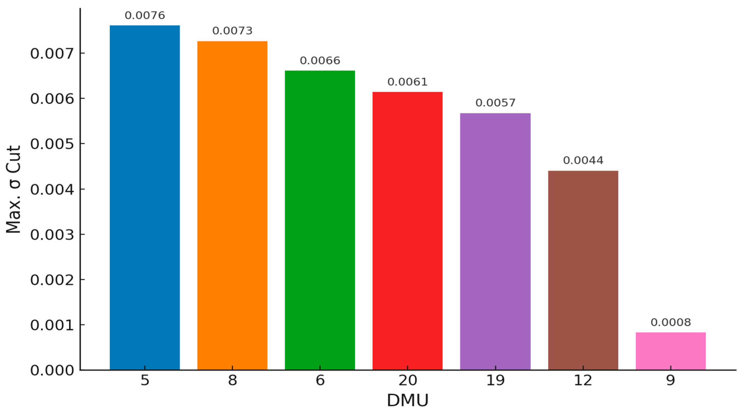
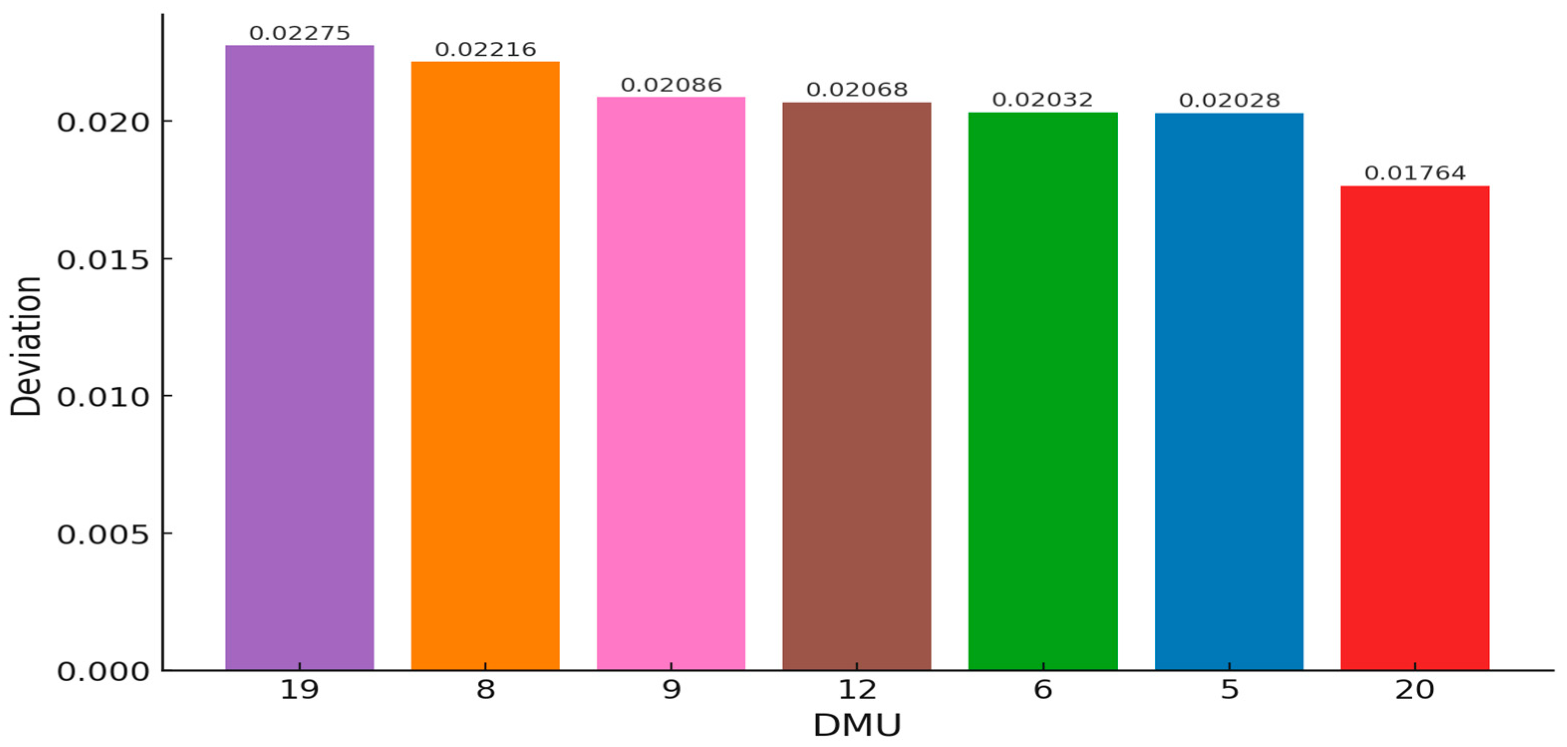
Two patterns stand out. First, the ordering by residual volatility differs from the raw inefficiency ranking: from lowest to highest residual, we obtain TC ≤ CI ≤ CP ≤ IF ≤ EP ≤ EC ≤ TO (DMUs 20, 5, 6, 12, 9, 8, 19). Thus, TC (Trading and Consumer Goods) can be steered closest to the frontier in risk terms after applying the maximum reduction, followed by CI and CP, whereas TO (Tourism) retains the largest residual volatility even after optimization, followed by EC and EP. Second, the gap between the minimum and maximum feasible cuts varies across industries, indicating different degrees of local slack versus full technology-wide risk-reduction potential. Together, these InvDEA outputs provide actionable targets for each underperforming portfolio: the minimum cut defines the efficiency-restoring “first mile,” and the maximum cut defines the technology-consistent “end state.” Graphical summaries in Figure 2 (volatility cut) and Figure 3 (residual deviations) visualize these results for benchmarking and managerial planning.

Figure 2. Feasible volatility cut bar plot.

Figure 3. Volatility deviation bar plot.

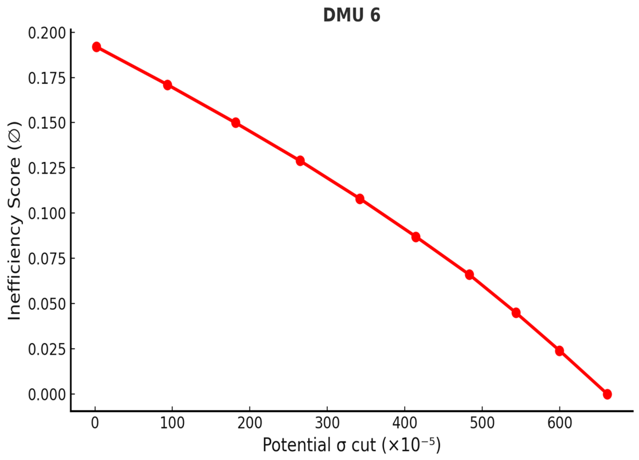
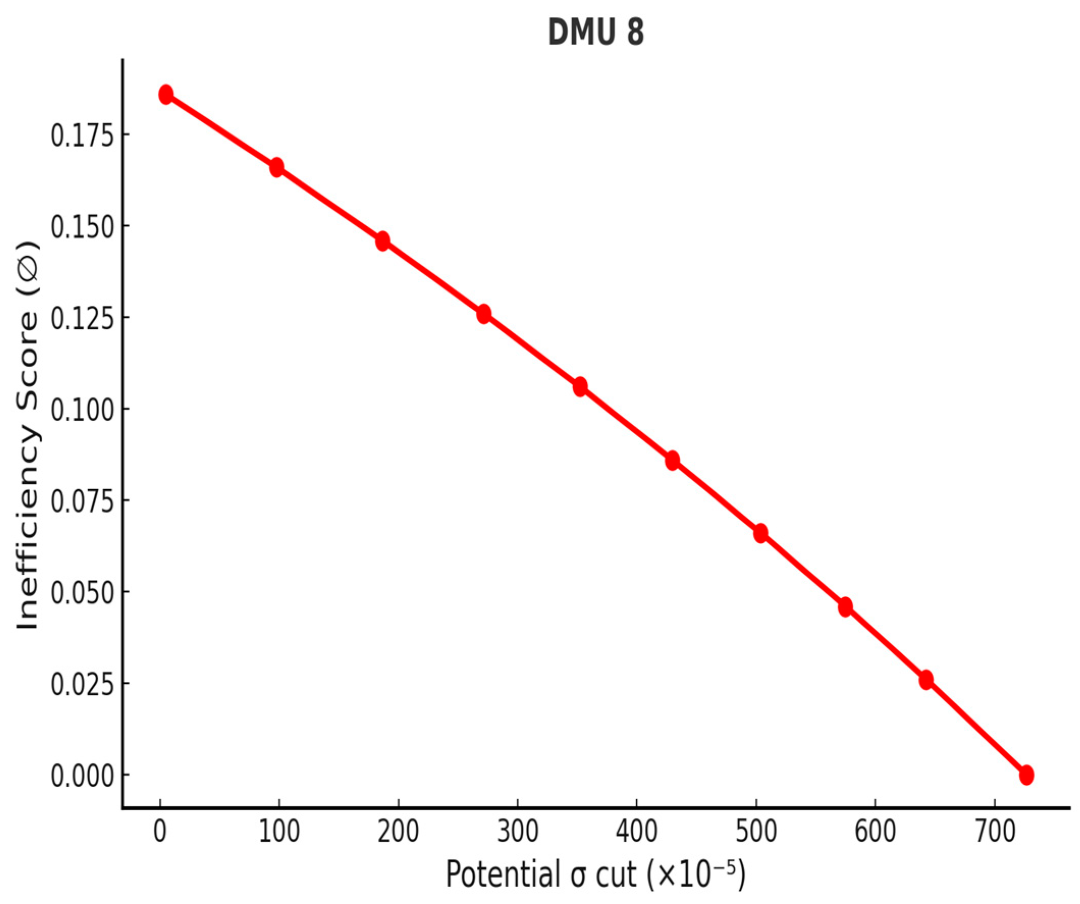
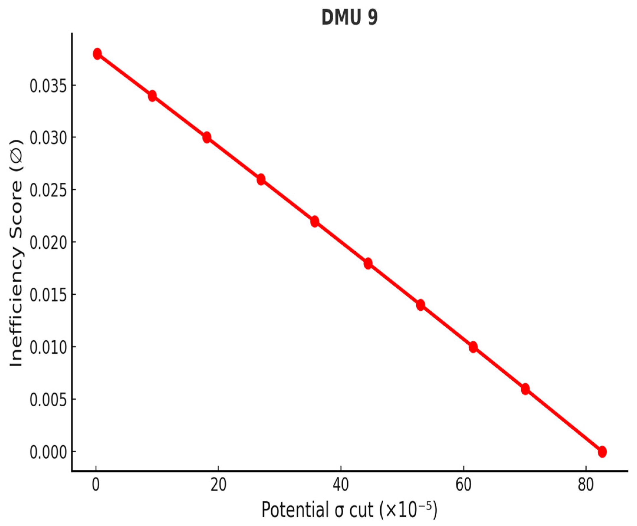
The analysis demonstrates that the proposed Inverse DEA framework can effectively mitigate volatility in inefficient portfolios. It should be noted, however, that the reductions estimated by the model represent theoretical maxima; in practice, the actual achievable decreases may be smaller due to market fluctuations and data uncertainties. Figure 4, Figure 5, Figure 6, Figure 7, Figure 8, Figure 9 and Figure 10 illustrate the relationship between inefficiency scores and volatility reduction, where scores were partitioned into equal intervals to trace the corresponding adjustment path. The resulting volatility curves confirm that the maximum reduction is always realized at the point where inefficiency is eliminated. By introducing this approach, the study provides a systematic method for estimating both feasible and maximum reductions in volatility, thereby enabling all inefficient portfolios in set B to attain efficiency. In doing so, the framework offers investors and managers a structured basis for setting realistic risk-reduction targets and making informed strategic decisions to enhance portfolio performance.

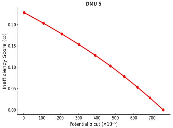
Figure 4. Volatility reduction curve—DMU 5.

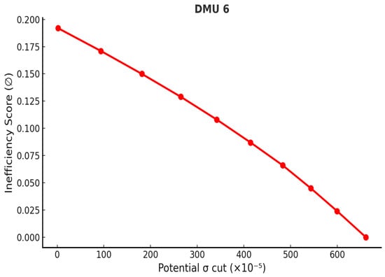
Figure 5. Volatility reduction curve—DMU 6.

Figure 6. Volatility reduction curve—DMU 8.

Figure 7. Volatility reduction curve—DMU 9.

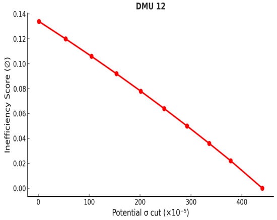
Figure 8. Volatility reduction curve—DMU 12.

Figure 9. Volatility reduction curve—DMU 19.

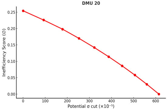
Figure 10. Volatility reduction curve—DMU 20.

Although the absolute volatility reductions appear numerically small (in the range of 0.0008–0.0076), they are significant when expressed in portfolio-scale risk terms. More importantly, within the DEA framework, these cuts are sufficient to eliminate all inefficiency, moving each underperforming portfolio to the efficient frontier.

4.3. Pre- and Post-COVID Regime Analysis

To further validate the robustness of our proposed Inverse DEA framework, we extend the analysis beyond the COVID-19 crisis year (2020) by incorporating both a pre-crisis calm regime (2019) and a post-crisis recovery regime (2021). The objective is to assess whether the model adapts sensibly across different market conditions, stable, stressed, and recovering, and whether its efficiency diagnostics and volatility-reduction targets remain consistent with economic intuition. Table 5, Table 6, Table 7, Table 8 and Table 9 present these results, including efficiency scores for 2019 and 2021, corresponding volatility cut analyses, and a consolidated comparison across the three years.

Table 5. 2019 Efficiency score results.

DMU	Industry	CR	AT	SR	R	σ	∅
1	AU	168.3755	0.6913	50.4835	0.142	0.01783	0
2	BM	417.2419	0.5303	34.3005	0.0984	0.01697	0
3	BU	1184.417	0.3372	56.3809	0.2024	0.01473	0
4	CH	274.6407	0.804	40.0614	0.0906	0.01508	0.0128
5	CI	301.361	0.8369	38.2367	0.259	0.02051	0
6	CP	217.2237	1.0508	45.4901	0.2012	0.01866	0
7	CC	293.0824	0.5884	39.0496	0.1465	0.0223	0
8	EC	253.0539	0.776	43.1949	0.2583	0.0204	0
9	EP	227.2874	2.0703	55.0632	0.1593	0.01434	0
10	EM	232.3705	0.666	44.11	0.0528	0.01614	0
11	FO	234.6261	0.9179	41.1532	0.0429	0.01238	0
12	IF	252.4844	1.045	40.2063	0.1656	0.01949	0
13	IS	215.4966	0.9311	49.2159	0.0246	0.01222	0
14	OE	261.2601	0.639	40.3925	0.1855	0.02202	0
15	PL	402.4628	0.7144	34.8824	0.0778	0.01328	0
16	SC	362.3101	0.738	31.9894	0.3673	0.02527	0
17	ST	159.5332	0.6893	59.7275	0.0841	0.01292	0
18	TX	642.5896	0.644	38.7975	0.0488	0.0158	0.1407
19	TO	185.2172	0.929	57.9303	0.0607	0.01918	0.3287
20	TC	292.1347	1.0156	52.2109	0.1011	0.01401	0.0429

Table 6. 2019 Volatility cut analysis (Pre-COVID-19).

DMU	Volatility (σ)	Potential σ Cut	Max. σ Cut	Deviation
4	0.01508	0.00001389	0.000229	0.014850
18	0.01580	0.00001298	0.002223	0.013576
19	0.01918	0.00002036	0.006540	0.012639
20	0.01401	0.00001475	0.000703	0.013306

Table 7. 2021 Efficiency score results.

DMU	Industry	CR	AT	SR	R	σ	∅
1	AU	177.9139	0.6776	50.2594	0.0258	0.02254	0
2	BM	525.1983	0.5025	32.6861	0.0658	0.02256	0
3	BU	203.6848	0.3448	61.1749	0.1633	0.0193	0
4	CH	254.9808	0.7858	39.8413	0.329	0.02364	0
5	CI	311.3627	0.7698	41.2931	0.1522	0.02621	0.2576
6	CP	200.7394	1.0541	48.5383	0.2507	0.02808	0.1468
7	CC	321.86	0.465	37.6129	0.1615	0.02669	0
8	EC	246.4232	0.8213	45.7866	0.3187	0.02805	0.1352
9	EP	185.6718	2.0538	58.1085	0.3663	0.02339	0
10	EM	217.3011	0.6791	46.3666	0.1712	0.02239	0
11	FO	212.2829	0.9143	41.1432	0.179	0.01689	0
12	IF	273.7689	0.9992	40.4905	0.2086	0.02488	0.194
13	IS	197.8907	1.0593	48.4251	0.4512	0.03327	0
14	OE	251.759	0.674	42.4803	0.3375	0.03163	0
15	PL	466.9524	0.7136	32.3364	0.1407	0.02322	0
16	SC	476.8166	0.7918	32.5843	0.5588	0.03536	0
17	ST	225.4054	0.7786	51.1514	0.7475	0.03894	0
18	TX	317.0738	0.6258	42.8383	0.1947	0.02608	0.1495
19	TO	212.6319	0.4033	54.5226	0.1065	0.02305	0
20	TC	355.664	0.918	53.3811	0.0751	0.02093	0.193

Table 8. 2021 Volatility cut analysis (Post COVID-19).

DMU	Volatility (σ)	Potential σ Cut	Max. σ Cut	Deviation
5	0.02621	0.00002533	0.007864	0.018346
6	0.02808	0.00003653	0.005964	0.022116
8	0.02805	0.00000710	0.005427	0.022623
12	0.02488	0.00004005	0.006554	0.018326
18	0.02608	0.00002005	0.004745	0.021335
20	0.02093	0.00002653	0.00404	0.016890

Table 9. Pre- and Post-COVID portfolio efficiency and volatility-reduction targets.

Year	Inefficient DMUs	∅ Range	Max. σ Cut Range
2019	4/20	0.0128–0.3287	0.000229–0.006540
2020	7/20	0.0381–0.2541	0.000827–0.007610
2021	6/20	0.1352–0.2576	0.004040–0.007864

The pre-COVID (2019) results (Table 5 and Table 6) reflect a stable market environment with generally higher efficiency and smaller volatility adjustments. Out of 20 DMUs, only 4 were inefficient, with inefficiency scores (∅) ranging from 0.0128 to 0.3287. The Inverse DEA-implied volatility reductions were modest, with maximum σ-cuts between 0.000229 and 0.006540. These findings align with expectations under calm market conditions, where portfolios operate closer to the efficient frontier and require only minor adjustments to volatility exposure. In contrast, the COVID crisis year (2020, see Table 3 and Table 4 earlier) exhibited a sharp deterioration, with 7 out of 20 DMUs classified as inefficient and higher σ-cuts of up to 0.007610, confirming the role of Inverse DEA as a stress-testing tool.

The post-COVID (2021) results (Table 7 and Table 8) capture a transitional recovery phase. Here, 6 of 20 DMUs were inefficient, with inefficiency scores ranging from 0.1352 to 0.2576. Although fewer industries were inefficient compared to 2020, the Inverse DEA-prescribed σ-cuts remained substantial, ranging from 0.004040 to 0.007864, larger than the 2019 calm levels. Table 9 consolidates these findings and illustrates a logical progression: fewer inefficiencies and smaller σ-cuts in 2019, more inefficiencies and larger σ-cuts in 2020, and intermediate results in 2021. This pattern suggests that while efficiency partially recovered after COVID, lingering inefficiencies persisted, reinforcing the practical value of Inverse DEA as a continuous monitoring and planning tool for risk management across regimes.

4.4. Feasibility Validation

Table 10 summary confirms that the proposed model M5 targets are theoretically consistent when the Inverse DEA-implied volatility reductions. In model M1, the initial risk values are replaced with new risk values, and are fed back into the original production set, then each previously inefficient industry portfolio becomes efficient. The projection lands on the frontier, an NZV efficient point is attained; otherwise, the portfolio achieves the lowest feasible residual risk without sacrificing return. Methodologically, this feasibility validation is an ex-post feasibility: it tests whether Inverse DEA targets derived from model M5 indeed satisfy the technological and efficiency constraints of model M1 when implemented in-sample. In practice, the Inverse DEA cuts represent theoretical maxima; actual achievable reductions may be smaller due to market frictions, execution constraints, or data uncertainty. The results in Table 10 provide strong evidence that our proposed Inverse DEA is internally valid and achieves its intended effect within the estimated technique.

Table 10. Validation analysis on portfolios.

DMU	Initial σ	Final σ	Initial ∅	Final ∅
5	0.02789	0.020280	0.2287	0
6	0.02693	0.020318	0.1924	0
8	0.02943	0.022163	0.1870	0
9	0.02169	0.020863	0.0381	0
12	0.02508	0.020679	0.1344	0
19	0.02842	0.022748	0.1995	0
20	0.02378	0.017640	0.2541	0

4.5. Managerial Implications

The proposed framework provides a clear, frontier-consistent roadmap for action. For each underperforming TWSE industry portfolio, managers obtain two horizons: a minimum volatility cut and a maximum feasible cut. The NZV initiative towards the minimum cut allows capturing some efficiency gains with limited disruption, while the gap to the maximum cut quantifies remaining headroom. Embedding these targets in portfolio guidelines, such as sector-level volatility caps, drawdown limits, and desk-level KPIs, aligns portfolios with feasible improvements and creates measurable accountability. Implementation should combine diversification adjustments, position sizing, hedging overlays, and exposure rebalancing to deliver the prescribed cuts without compromising returns. Importantly, the volatility-reduction targets do not yield investable weights directly; rather, they provide frontier-consistent σ-caps that establish feasible risk budgets, allowing managers to integrate them within existing allocation frameworks. Hence, the Inverse DEA outputs translate theoretical reductions into actionable guidelines, ensuring that resulting allocations are both efficiency-consistent and implementable within existing portfolio management frameworks.

The pre- and post-COVID regime analysis reinforces these implications by showing that Inverse DEA adapts sensibly across different market conditions. In the calm pre-crisis period (2019), inefficiency was limited and σ-caps implied only modest volatility reductions. During the crisis year (2020), inefficiencies widened and required larger σ-cuts, highlighting Inverse DEA’s role as a stress-testing tool. The recovery year (2021) showed partial normalization, with inefficiency levels reduced compared to 2020 but still above pre-crisis levels, requiring intermediate adjustments. This logical progression suggests that managers can use Inverse DEA dynamically, tightening volatility caps in stressed regimes, relaxing them in stable periods, and applying moderate cuts in recovery phases. Such regime-specific monitoring and adjustment provides a transparent audit trail from diagnosis (excess risk) to remedy (targeted volatility reduction), supporting effective investment governance and regulatory communication.

5. Conclusions and Future Study

This study develops and tests an inverse optimization framework for portfolio risk management. Building on a DDF–DEA model that treats return as a desirable output and volatility as an undesirable one, we aggregate 1365 TWSE equities into 20 industry portfolios and identify their technology-consistent improvement paths. The DDF–DEA baseline (M1) classifies 13 portfolios as efficient and 7 as inefficient, revealing heterogeneous distances to the frontier. We then formulate an inverse model (M5) that prescribes feasible volatility cuts at the current return level. The model delivers two actionable targets for each underperformer: the minimum cut possible and the maximum feasible cut to reach the efficient frontier. A post-feasibility validation confirms the internal coherence of these prescriptions. Substituting the Inverse DEA-implied volatility values back into (M1) drives all previously inefficient portfolios to the frontier, demonstrating that the proposed reductions are production-set consistent rather than aspirational artifacts. Together with the industry-level ranking by residual (post-cut) risk, the framework provides managers a transparent, frontier-aligned basis for risk budgeting, sequencing of hedges and rebalancing, and embedding efficiency-restoring targets into governance. Importantly, the “net-zero” notion functions as a theoretical bound, clarifying the edge of what the observed technology permits without presuming that markets can consistently deliver the full cut.

In addition, we extend the analysis across market regimes to test the robustness of the framework. The pre-crisis calm year (2019) exhibited fewer inefficiencies and smaller volatility-reduction targets, while the crisis year (2020) revealed broader inefficiencies and larger σ-cuts. The recovery year (2021) showed partial normalization, with intermediate efficiency levels and volatility reductions, suggesting that Inverse DEA adapts logically across stable, stressed, and transitional environments. This regime sensitivity enhances the managerial value of the framework, showing that it can function not only as a stress-test tool but also as a continuous monitoring mechanism for aligning portfolios with efficiency-consistent risk budgets under evolving conditions.

These contributions come with limitations. Although we extend the analysis across three regimes, our results remain in-sample and anchored to historical data. The framework does not yet account for forward-looking market swings, structural shifts, or predictive dynamics. We recommend further research to explore effective managerial or predictive techniques for achieving the identified risk reduction. Furthermore, due to the annual surge in new stock debuts, it may be challenging to replicate this model to cover the latest datasets of equities, and as such, our approach may be time-consuming and energy-demanding. Future extensions of this research could incorporate ESG and macroeconomic indicators, provided sufficiently large and harmonized datasets are available. The possible integration of Inverse DEA with emerging machine learning, deep learning or blockchain technologies (Choi et al., 2021; T. Kehinde et al., 2025; T. O. Kehinde et al., 2025a; Khan, 2023; Khan et al., 2025; Khan et al., 2020) for business or financial intelligence is an opportunity for future research directions, offering potential breakthroughs in informed business decision-making. In summary, this research establishes a distinct line of work within Inverse DEA applications for stock portfolio evaluation, offering a crucial, regime-sensitive tool for informed financial decision-making.

References

- Akbarian, D., & Oukil, A. (2025). Improving efficiency evaluation in the presence of ratio data: Inverse non-radial Enhanced Russell Models. IMA Journal of Management Mathematics, 36(2), 339–362. [Google Scholar] [CrossRef]
- Amin, G. R., & Al-Muharrami, S. (2018). A new inverse data envelopment analysis model for mergers with negative data. IMA Journal of Management Mathematics, 29(2), 137–149. [Google Scholar] [CrossRef]
- Amin, G. R., Al-Muharrami, S., & Toloo, M. (2019). A combined goal programming and inverse DEA method for target setting in mergers. Expert Systems with Applications, 115, 412–417. [Google Scholar] [CrossRef]
- Amin, G. R., Emrouznejad, A., & Gattoufi, S. (2017a). Minor and major consolidations in inverse DEA: Definition and determination. Computers and Industrial Engineering, 103, 193–200. [Google Scholar] [CrossRef]
- Amin, G. R., Emrouznejad, A., & Gattoufi, S. (2017b). Modelling generalized firms’ restructuring using inverse DEA. Journal of Productivity Analysis, 48(1), 51–61. [Google Scholar] [CrossRef]
- Amin, G. R., & Ibn-Boamah, M. (2021). A two-stage inverse data envelopment analysis approach for estimating potential merger gains in the US banking sector. Managerial and Decision Economics, 42(6), 1454–1465. [Google Scholar] [CrossRef]
- Amin, G. R., & Ibn-Boamah, M. (2023). Modeling business partnerships: A data envelopment analysis approach. European Journal of Operational Research, 305(1), 329–337. [Google Scholar] [CrossRef]
- Amin, G. R., & Oukil, A. (2019). Flexible target setting in mergers using inverse data envelopment analysis. International Journal of Operational Research, 35(3), 301–317. [Google Scholar] [CrossRef]
- Amirteimoori, A., & Allahviranloo, T. (2024). Improving technical efficiency in data envelopment analysis for efficient firms: A case on Chinese banks. Information Sciences, 681, 121237. [Google Scholar] [CrossRef]
- An, Q., Liu, X., Li, Y., & Xiong, B. (2019). Resource planning of Chinese commercial banking systems using two-stage inverse data envelopment analysis with undesirable outputs. PLoS ONE, 14(6), e0218214. [Google Scholar] [CrossRef]
- Andria, J., di Tollo, G., & Lokketangen, A. (2017). Distance measures for portfolio selection. In Financial decision aid using multiple criteria: Recent models and applications (pp. 113–129). Springer. [Google Scholar][Green Version]
- Andria, J., Di Tollo, G., & Pesenti, R. (2021). Fuzzy multi-criteria decision-making: An entropy-based approach to assess tourism sustainability. Tourism Economics, 27(1), 168–186. [Google Scholar]
- Asadi, F., Kordrostami, S., Amirteimoori, A., & Bazrafshan, M. (2023). Inverse data envelopment analysis without convexity: Double frontiers. Decisions in Economics and Finance, 46(1), 335–354. [Google Scholar] [CrossRef]
- Basso, A., & Funari, S. (2001). A data envelopment analysis approach to measure the mutual fund performance. European Journal of Operational Research, 135(3), 477–492. [Google Scholar] [CrossRef]
- Bauder, D., Bodnar, T., Parolya, N., & Schmid, W. (2021). Bayesian mean–variance analysis: Optimal portfolio selection under parameter uncertainty. Quantitative Finance, 21(2), 221–242. [Google Scholar]
- Caldeira, J. F., Santos, A. A., & Torrent, H. S. (2023). Semiparametric portfolios: Improving portfolio performance by exploiting non-linearities in firm characteristics. Economic Modelling, 122, 106239. [Google Scholar] [CrossRef]
- Choi, T.-M., Chung, S.-H., Sun, X., & Wen, X. (2021). Using blockchain to improve buffer-stock-sharing and combat cheating behaviors under virtual pooling. IEEE Transactions on Engineering Management, 71, 328–345. [Google Scholar]
- Chung, Y. H., Färe, R., & Grosskopf, S. (1997). Productivity and undesirable outputs: A directional distance function approach. Journal of Environmental Management, 51(3), 229–240. [Google Scholar] [CrossRef]
- Daryani, Z. S., Tohidi, G., Daneshian, B., Razavyan, S., & Hosseinzadeh Lotfi, F. H. (2021). Inverse DEA in two-stage systems based on allocative efficiency. Journal of Intelligent and Fuzzy Systems, 40(1), 591–603. [Google Scholar] [CrossRef]
- Ebrahimi, M., Valami, H. B., & Karamali, L. (2021). Portfolio Selection by a Non-Radial DEA Model: Evidence from of Tehran Stock Exchange (TSE). Journal of Mathematics and Modeling in Finance, 1(2), 181–193. [Google Scholar]
- Edirisinghe, N. C. P., & Zhang, X. (2008). Portfolio selection under DEA-based relative financial strength indicators: Case of US industries. Journal of the Operational Research Society, 59, 842–856. [Google Scholar] [CrossRef]
- Emrouznejad, A., & Amin, G. R. (2023). Advances in inverse data envelopment analysis: Empowering performance assessment. IMA Journal of Management Mathematics, 34(3), 415–419. [Google Scholar] [CrossRef]
- Emrouznejad, A., Amin, G. R., Ghiyasi, M., & Michali, M. (2023). A review of inverse data envelopment analysis: Origins, development and future directions. IMA Journal of Management Mathematics, 34(3), 421–440. [Google Scholar] [CrossRef]
- Galagedera, D. U. A. (2024). Planning for potential increases in disbursements and risk of managed funds conditional on desired short-term performance levels. Applied Economics, 56(28), 3385–3400. [Google Scholar] [CrossRef]
- Gattoufi, S., Amin, G. R., & Emrouznejad, A. (2014). A new inverse DEA method for merging banks. IMA Journal of Management Mathematics, 25(1), 73–87. [Google Scholar] [CrossRef]
- Gerami, J., Mozaffari, M. R., Wanke, P. F., & Corrêa, H. L. (2023). A generalized inverse DEA model for firm restructuring based on value efficiency. IMA Journal of Management Mathematics, 34(3), 541–580. [Google Scholar] [CrossRef]
- Ghiyasi, M. (2024). An inverse data envelopment analysis model for solving time substitution problems. Decision Analytics Journal, 11, 100467. [Google Scholar] [CrossRef]
- Ghiyasi, M. (2025). New insights and theoretical conditions for determining minor and major consolidations in the inverse DEA. IMA Journal of Management Mathematics, 36(3), 563–578. [Google Scholar] [CrossRef]
- Ghiyasi, M., & Zhu, N. (2020). An inverse semi-oriented radial data envelopment analysis measure for dealing with negative data. IMA Journal of Management Mathematics, 31(4), 505–516. [Google Scholar] [CrossRef]
- Ghiyasi, M., & Zhu, N. (2025). Inverse data envelopment analysis for parallel production systems: An analysis in four types of Chinese banks. International Journal of System Assurance Engineering and Management, 16(1), 29–37. [Google Scholar] [CrossRef]
- Ghobadi, S. (2021). Merging decision-making units with interval data. RAIRO—Operations Research, 55, S1605–S1631. [Google Scholar] [CrossRef]
- Ghobadi, S., Soleimani-Chamkhorami, K., & Zanboori, E. (2023). Simultaneous estimation of input–output levels under improving efficiency level in an assessment window. Soft Computing, 27(8), 4553–4577. [Google Scholar] [CrossRef]
- Ghomi, A., Ghobadi, S., Behzadi, M. H., & Rostamy-Malkhlifeh, M. (2021). Inverse data envelopment analysis with stochastic data. RAIRO—Operations Research, 55(5), 2739–2762. [Google Scholar] [CrossRef]
- Guijarro, F., Martínez-Gómez, M., & Visbal-Cadavid, D. (2020). A model for sector restructuring through genetic algorithm and inverse DEA. Expert Systems with Applications, 154, 113422. [Google Scholar] [CrossRef]
- Hosseinzadeh Lotfi, F. H., Ghazi, N. E., Ghazi, S. E., & Namin, M. A. (2012). The outputs estimation of a DMU according to improvement of its progress in context dependent DEA. Applied Mathematical Sciences, 6(5–8), 247–258. Available online: https://www.scopus.com/inward/record.uri?eid=2-s2.0-84856584121&partnerID=40&md5=98dd03a645023acec84f852884c2583c (accessed on 15 January 2025).
- Ibn-Boamah, M., & Amin, G. R. (2024). Partner selection in business mergers: A data envelopment analysis approach. RAIRO—Operations Research, 58(4), 3107–3117. [Google Scholar] [CrossRef]
- Jing, D., Imeni, M., Edalatpanah, S. A., Alburaikan, A., & Khalifa, H. A. E.-W. (2023). Optimal selection of stock portfolios using multi-criteria decision-making methods. Mathematics, 11(2), 415. [Google Scholar]
- Kehinde, T., Adedokun, O. J., Joseph, A., Kabirat, K. M., Akano, H. A., & Olanrewaju, O. A. (2025). Helformer: An attention-based deep learning model for cryptocurrency price forecasting. Journal of Big Data, 12(1), 81. [Google Scholar] [CrossRef]
- Kehinde, T., Chan, F. T., & Chung, S. (2023a). Scientometric review and analysis of recent approaches to stock market forecasting: Two decades survey. Expert Systems with Applications, 213, 119299. [Google Scholar]
- Kehinde, T., Chung, S., & Chan, F. T. (2023b, July 13–14). Benchmarking TPU and GPU for stock price forecasting using LSTM model development. Science and Information Conference, London, UK. [Google Scholar]
- Kehinde, T., Khan, W. A., & Chung, S.-H. (2023c, October 10–12). Financial market forecasting using RNN, LSTM, BiLSTM, GRU and transformer-based deep learning algorithms. IEOM International Conference on Smart Mobility and Vehicle Electrification, Detroit, MI, USA. [Google Scholar]
- Kehinde, T. O., Adedokun, O. J., Kareem, M. K., Akpan, J., & Olanrewaju, O. A. (2025a). STL-ELM: A computationally efficient hybrid approach for predicting high volatility stock market. Intelligent Systems with Applications, 27, 200564. [Google Scholar] [CrossRef]
- Kehinde, T. O., Chung, S. H., & Olanrewaju, O. A. (2025b). An integrated approach to stock selection and ranking: Combining Shannon entropy technique, DEA, and inverse DEA. IEEE Access, 13, 138851–138866. [Google Scholar] [CrossRef]
- Khan, W. A. (2023). Balanced weighted extreme learning machine for imbalance learning of credit default risk and manufacturing productivity. Annals of Operations Research, 348, 833–861. [Google Scholar] [CrossRef]
- Khan, W. A., Chung, S. H., Awan, M. U., & Wen, X. (2020). Machine learning facilitated business intelligence (Part II) Neural networks optimization techniques and applications. Industrial Management & Data Systems, 120(1), 128–163. [Google Scholar]
- Khan, W. A., Chung, S.-H., Liu, S. Q., Masoud, M., & Wen, X. (2025). Smoothing and Matrix decomposition-based stacked bidirectional GRU model for machine downtime forecasting. IEEE Transactions on Systems, Man, and Cybernetics: Systems, 55(10), 7215–7227. [Google Scholar] [CrossRef]
- Kuo, K.-C., Lu, W.-M., & Dinh, T. N. (2021). An integrated efficiency evaluation of China stock market. Journal of the Operational Research Society, 72(4), 950–969. [Google Scholar] [CrossRef]
- Markowitz, H. M. (1991). Foundations of portfolio theory. The Journal of Finance, 46(2), 469–477. [Google Scholar] [CrossRef]
- Mergoni, A., Emrouznejad, A., & De Witte, K. (2024). Fifty years of data envelopment analysis. European Journal of Operational Research, 326(3), 389–412. [Google Scholar] [CrossRef]
- Oloko, T. F. (2018). Portfolio diversification between developed and developing stock markets: The case of US and UK investors in Nigeria. Research in International Business and Finance, 45, 219–232. [Google Scholar] [CrossRef]
- Orisaremi, K. K., Chan, F. T. S., & Chung, N. S. H. (2021). Potential reductions in global gas flaring for determining the optimal sizing of gas-to-wire (GTW) process: An inverse DEA approach. Journal of Natural Gas Science and Engineering, 93, 103995. [Google Scholar] [CrossRef]
- Panwar, A., Olfati, M., Pant, M., & Snasel, V. (2022). A review on the 40 years of existence of data envelopment analysis models: Historic development and current trends. Archives of Computational Methods in Engineering, 29(7), 5397–5426. Available online: https://pmc.ncbi.nlm.nih.gov/articles/PMC9184254/pdf/11831_2022_Article_9770.pdf (accessed on 15 January 2025). [CrossRef]
- Peykani, P., Seyed Esmaeili, F. S., Mirmozaffari, M., Jabbarzadeh, A., & Khamechian, M. (2022). Input/output variables selection in data envelopment analysis: A shannon entropy approach. Machine Learning and Knowledge Extraction, 4(3), 688–699. [Google Scholar] [CrossRef]
- Pirgaip, B., Ertuğrul, H. M., & Ulussever, T. (2021). Is portfolio diversification possible in integrated markets? Evidence from South Eastern Europe. Research in International Business and Finance, 56, 101384. [Google Scholar] [CrossRef]
- Sohrabi, A., Gerami, J., & Mozaffari, M. R. (2024). A novel approach for modelling strategic alliances and partnerships based on the DEA-R models. Japan Journal of Industrial and Applied Mathematics, 41(3), 1629–1678. [Google Scholar] [CrossRef]
- Soleimani-Chamkhorami, K., Hosseinzadeh Lotfi, F., Jahanshahloo, G., & Rostamy-Malkhlifeh, M. (2020). A ranking system based on inverse data envelopment analysis. IMA Journal of Management Mathematics, 31(3), 367–385. [Google Scholar] [CrossRef]
- Soleimani-Chamkhorami, K., Hosseinzadeh Lotfi, F. H., Jahanshahloo, G. R., & Rostamy-Malkhlifeh, M. (2019). Preserving cost and revenue efficiency through inverse data envelopment analysis models. INFOR, 58(4), 561–578. [Google Scholar] [CrossRef]
- Soltanifar, M., Ghiyasi, M., Emrouznejad, A., & Sharafi, H. (2024). A novel model for merger analysis and target setting: A CSW-Inverse DEA approach. Expert Systems with Applications, 249, 123326. [Google Scholar] [CrossRef]
- Soltanifar, M., Ghiyasi, M., & Sharafi, H. (2023). Inverse DEA-R models for merger analysis with negative data. IMA Journal of Management Mathematics, 34(3), 491–510. [Google Scholar] [CrossRef]
- Soltanifar, M., Tavana, M., Charles, V., Ghiyasi, M., & Sharafi, H. (2025). A novel inverse data envelopment analysis model with negative ratio data. Operational Research, 25(2), 25. [Google Scholar] [CrossRef]
- Statista. (2023). Total market capitalizations of domestic companies listed on stock exchanges worldwide from 2013 to July 2023. Statista. Available online: https://www.statista.com/statistics/274490/global-value-of-share-holdings-since-2000/#:~:text=As%20of%20July%202023%2C%20the,world%20stocks%20as%20of%202023 (accessed on 16 December 2023).
- Tarnaud, A. C., & Leleu, H. (2018). Portfolio analysis with DEA: Prior to choosing a model. Omega, 75, 57–76. [Google Scholar] [CrossRef]
- Trichilli, Y., Abbes, M. B., & Masmoudi, A. (2020). Islamic and conventional portfolios optimization under investor sentiment states: Bayesian vs. Markowitz portfolio analysis. Research in International Business and Finance, 51, 101071. [Google Scholar] [CrossRef]
- Wang, W., Jingyun, L., Bin, L., Wang, W., Zhang, Z., Kaining, S., & Mao, F. (2023). Effectiveness and risk of initial carbon quota allocation principle under the uncertainty of the Chinese electricity market. China Economic Review, 77, 101892. [Google Scholar] [CrossRef]
- Wegener, M., & Amin, G. R. (2019). Minimizing greenhouse gas emissions using inverse DEA with an application in oil and gas. Expert Systems with Applications, 122, 369–375. [Google Scholar] [CrossRef]
- Wei, Q., Zhang, J., & Zhang, X. (2000). An inverse DEA model for inputs/outputs estimate. European Journal of Operational Research, 121(1), 151–163. [Google Scholar] [CrossRef]
- Wijaya, W., & Sidarto, K. A. (2023). Large-scale portfolio optimization using biogeography-based optimization. International Journal of Financial Studies, 11(4), 125. [Google Scholar] [CrossRef]
- Xie, Q., Dai, Q., Li, Y., & Jiang, A. (2014). Increasing the discriminatory power of DEA using Shannon’s entropy. Entropy, 16(3), 1571–1585. [Google Scholar] [CrossRef]
- Yadav, M. P., Sharif, T., Ashok, S., Dhingra, D., & Abedin, M. Z. (2023). Investigating volatility spillover of energy commodities in the context of the Chinese and European stock markets. Research in International Business and Finance, 65, 101948. [Google Scholar] [CrossRef]
- Yu, A., Shao, Y., You, J., Wu, M., & Xu, T. (2019). Estimations of operational efficiencies and potential income gains considering the credit risk for China’s banks. Journal of the Operational Research Society, 70(12), 2153–2168. [Google Scholar] [CrossRef]
- Zeinodin, E., & Ghobadi, S. (2020). Merging decision-making units under inter-temporal dependence. IMA Journal of Management Mathematics, 31(2), 139–166. [Google Scholar] [CrossRef]
- Zeng, X., Zhou, Z., Gong, Y., & Liu, W. (2022). A data envelopment analysis model integrated with portfolio theory for energy mix adjustment: Evidence in the power industry. Socio-Economic Planning Sciences, 83, 101332. [Google Scholar] [CrossRef]
- Zhou, B. (2023). The impact of the US Chip Act and the Chip4 Alliance, and China how to respond it. Transactions on Social Science, Education and Humanities Research, 1, 407–410. [Google Scholar]
Disclaimer/Publisher’s Note: The statements, opinions and data contained in all publications are solely those of the individual author(s) and contributor(s) and not of MDPI and/or the editor(s). MDPI and/or the editor(s) disclaim responsibility for any injury to people or property resulting from any ideas, methods, instructions or products referred to in the content. |
© 2025 by the authors. Licensee MDPI, Basel, Switzerland. This article is an open access article distributed under the terms and conditions of the Creative Commons Attribution (CC BY) license (https://creativecommons.org/licenses/by/4.0/).