To Burn-In, or Not to Burn-In: That’s the Question

Abstract

In this paper it is shown that the bathtub-curve (BTC) based time-derivative of the failure rate at the initial moment of time can be considered as a suitable criterion of whether burn-in testing (BIT) should or does not have to be conducted. It is also shown that the above criterion is, in effect, the variance of the random statistical failure rate (SFR) of the mass-produced components that the product manufacturer received from numerous vendors, whose commitments to reliability were unknown, and their random SFR might vary therefore in a very wide range, from zero to infinity. A formula for the non-random SFR of a product comprised of mass-produced components with random SFRs was derived, and a solution for the case of the normally distributed random SFR was obtained.

1. Introduction

Burn-in testing (BIT) [1,2,3,4,5,6,7,8,9,10] has for many years been an accepted practice for detecting and eliminating early failures in newly fabricated electronic products prior to shipping the “healthy” ones that survived BIT to customers. BIT is mandatory on most high-reliability procurement contracts, such as for military and aerospace applications, but is also a must for automotive, medical, long-haul telecommunication and other electronic materials, packages and systems, whose high operational performance is paramount. BIT stimulates failures in defective materials and vulnerable structural elements of the manufactured products by accelerating the stresses that will supposedly cause these materials and elements to fail. BIT is usually conducted at the component level, because the cost of testing and replacing parts is the lowest at this level. The products are tested by applying stress extremes, usually, but not necessarily, of the expected operational stressors. It is believed that once a sufficiently long BIT process is complete, no further early failures are likely to occur.

Depending on the anticipated operation conditions of the product and testing capabilities of a particular manufacturer, BIT can be based on temperature cycling, elevated temperatures, voltage, current, humidity, random vibrations, and so on, or, since the principle of superposition does not work in the reliability engineering—on the appropriate combination of these stressors. The duration of stressing depends on the product, the manufacturing technology and the reliability requirements, with consideration of the consequences of possible failures. Elevated temperature (say, 125 °C for 168 h) or elevated stresses screening (say, twenty temperature cycles from −10 °C to 70 °C) are most often used. For complex products, dynamic BIT might be employed. The thermal stress, caused by the change in temperature, is combined in these tests with dynamic (shocks, random vibrations) loading. Such a temperature-dynamic bias is thought to provide worst-case operating conditions [11,12]. For commercial applications, BIT, if any is conducted at all, does not last longer than one or two days (24 or 48 h). BIT is a costly effort, and its application is therefore thoroughly planned and carefully executed.

It goes without saying that as a result of successfully applying BIT, early failures are avoided and the infant mortality portion (IMP) of the bathtub-curve (BTC) (Figure 1) is eliminated at the expense of an undesirable reduced yield caused by the BIT process. In addition, high BIT stresses might not only eliminate “freaks”, but could cause permanent damage to the main population of the “healthy” products, thereby reducing their lifetime. It is unclear, however, to what extent it happens indeed: the highly accelerated life testing (HALT) [13], a “black box” that tries “to kill many birds with one stone” and is at present the testing procedure of choice employed as a suitable BIT vehicle, is unable to provide any information on that.

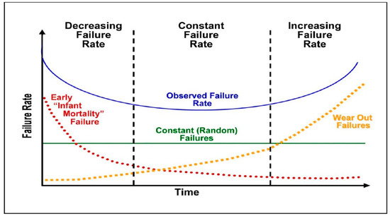
Figure 1. Bathtub curve—“reliability passport” of an electronic product.

It remains unclear what could possibly be done to develop an insight into what is actually happening during and as a result of BIT and what could possibly be done to effectively eliminate “freaks”, while shortening the testing time and not damaging the sound devices. In a mature production, when HALT is relied upon to do the BIT job, it is not easy even to determine whether there exists a decreasing failure rate. To determine the failure time for a very low percentage of the production, one has to destroy a large number of devices, unless there are additional considerations of what could be possibly done to enhance the merits of the BIT process and to minimize its shortcomings. Thus, there is an obvious incentive to develop ways in which the BIT process could be quantified, monitored and possibly optimized. Accordingly, in this analysis some important aspects of BIT are addressed for an electronic product comprised of numerous mass-produced components. Our intent is to shed some quantitative light on the BIT process. Particularly, we try to develop a suitable and predictable criterion that would be able to answer the fundamental “to burn-in or not to burn-in” question.

Two mutually complementing modeling studies have been carried out here: (1) the analysis of the configuration of the IMP of a BTC of a more or less well established manufacturing technology; and (2) the analysis of the role of the random statistical failure rate (SFR) of the mass-produced components that the product of interest is comprised of. Particularly, as far as the second study is concerned, we consider the effect that the random SFR of the mass-produced components might have on the nonrandom initial SFR of the product. Although this paper does not offer a straightforward and an ultimate answer to the “to burn-in or not to burn-in” question, nor to how to optimize the BIT process, in terms of its cost and duration, the suggested physics-of-failure and statistics-of-failure based criterion, and the calculated probabilities of non-failure for the given loading conditions and time of testing provide, in our judgment, a useful step forward in advancing the state-of-the-art in today’s BIT practice.

BIT, being an HALT effort, is, in effect, a failure-oriented-accelerated-test (FOAT) [14,15,16] and, as such, should be geared, to confirm the anticipated physics of failure and the expected failure modes, to a physically meaningful accelerated test model. The application of the probabilistic design for reliability (PDfR) approach [17,18] and its constituents, FOAT and multi-parametric Boltzmann-Arrhenius-Zhurkov’s equation (BAZ) [19,20,21], are beyond the scope of this paper. The PDfR/FOAT/BAZ concept is considered, however, as important future work. Let us briefly elaborate on its substance.

If the well-known Arrhenius model [22] is employed, FOAT should be conducted to determine the corresponding activation energies and other data that characterize the device reliability [23]. The desirable steady-state portion of the BTC occurs, as is known, at the end of the BIT process as a result of the interaction of two major irreversible processes: the “favorable” SFR process, resulting in a decreasing failure rate with time, and the “unfavorable” physics-of-failure-related process (PFR), resulting in an increasing failure rate. The first process dominates at the IMP of the BTC and is considered in this paper, and the second one—at its wear-out portion. These two processes start to compensate for each other at the beginning of the low enough and acceptable level ${\lambda }_0$ of the steady-state BTC failure rate process. The SFR process can be predicted [24,25] for a product comprised of mass-produced components, from sheer theoretical considerations. Assuming that the physics-of-failure and statistics-of-failure processes are statistically independent, the failure rates of the first process at the given moment of time can be obtained by simply deducting the predicted SFR values from the experimentally obtained BTC ordinates. In our BIT analysis, a different application of the Ref. [24,25] finding is employed, namely, to quantify, on the probabilistic basis, some more or less well known considerations underlying the existing BIT practice, including the “to burn-in, or not to burn-in” question. Application of the PDfR/FOAT/BAZ concept will be able, hopefully, not only answer this question for the given manufacturing technology, but, most importantly, will be able to establish the appropriate elevated stresses and their levels, and decide on the effective BIT duration to minimize the number of devices that will be destroyed and the time of testing. The numerical example in Appendix B gives an indication of what could be expected from the application of the PDfR/FOAT/BAZ concept.

2. Analysis

2.1. Prediction Based on the Analytical Approximation of the Bathtub-Curve (BTC)

The typical BTC, the “reliability passport” of a mass-produced electronic product (Figure 1), can be approximated by the following expressions [18]:

$$\lambda (t)=\{\begin{array}{l}{\lambda }_0+({\lambda }_1-{\lambda }_0){\left(1-\frac{t}{t_1}\right)}^{n_1}={\lambda }_0\left[1+\left(\frac{{\lambda }_1}{{\lambda }_0}-1\right){\left(1-\frac{t}{t_1}\right)}^{n_1}\right],0\le t\le t_1\\ {\lambda }_0+({\lambda }_2-{\lambda }_0){\left(\frac{t-t_1}{t_2}\right)}^{n_2}={\lambda }_0\left[1+\left(\frac{{\lambda }_2}{{\lambda }_0}-1\right){\left(\frac{t}{t_2}-\frac{t_1}{t_2}\right)}^{n_2}\right],t_1\le t\le t_1+t_2\end{array}$$

(1)

Here $\lambda (t)$ is time-dependent failure rate, ${\lambda }_0$ is its steady-state minimum, ${\lambda }_1$ is its initial (high) value at the beginning of the IMP, $t_1$ is the duration of this portion, ${\lambda }_2$ is the final (actual or acceptable) value of the failure rate at the end of the wear-out portion, $t_2$ is the duration of this portion, and the exponents $n_1$ and $n_2$ are expressed through the fullnesses ${\beta }_1$ and ${\beta }_2$ of the BTC infant-mortality and the wear-out portions as $n_{1,2}=\frac{{\beta }_{1,2}}{1-{\beta }_{1,2}}$. These fullnesses are defined as the ratios of the areas below the BTC (i.e., the areas between the BTC and the time axis) to the areas $({\lambda }_1-{\lambda }_0)t_1$ and $({\lambda }_2-{\lambda }_0)t_2$ of the corresponding rectangulars. The exponents $n_1$ and $n_2$ change from zero to one, when the fullnesses ${\beta }_1$ and ${\beta }_2$ change from zero to 0.5. The “to burn-in or not to burn-in” question can be tentatively answered based on the derivative:

$${\lambda }^{\prime }(t)=\frac{d\lambda (t)}{dt}=-\frac{{\lambda }_1-{\lambda }_0}{t_1}{n}_1{\left(1-\frac{t}{t_1}\right)}^{n_1-1}=-\frac{{\lambda }_1-{\lambda }_0}{t_1}\frac{{\beta }_1}{1-{\beta }_1}{\left(1-\frac{t}{t_1}\right)}^{\frac{2{\beta }_1-1}{1-{\beta }_1}}$$

(2)

calculated for the initial moment of time $t=0$. This yields:

$${\lambda }^{\prime }(0)=\frac{d\lambda (t)}{dt}=-\frac{{\lambda }_1-{\lambda }_0}{t_1}\frac{{\beta }_1}{1-{\beta }_1}.$$

(3)

If this derivative is zero or next-to-zero, this means that there is no IMP at all, so that no BIT is needed to eliminate this portion, and “not to burn-in” is the answer to our basic question. This certainly happens when the initial value ${\lambda }_1$ of the BTC is not different from its steady-state ${\lambda }_0$ value. What is less obvious is that the same result takes place for $\frac{{\beta }_1}{t_1}=0$. This means that no more or less durable BIT is needed in such a case, because there are not too many “freaks” in the population, and that these “freaks” are characterized by very low probabilities of non-failure, so that the planned BIT process is a next-to-instantaneous one. The maximum value of the fullness ${\beta }_1$ is ${\beta }_1=0.5$. This corresponds to the case when the IMP of the BTC is a straight line connecting the initial, ${\lambda }_1,$ and the steady-state, ${\lambda }_0,$ values of the BTC. In this case,

$${\lambda }^{\prime }(0)=\frac{d\lambda (t)}{dt}=-\frac{{\lambda }_1-{\lambda }_0}{t_1}.$$

(4)

The derivative (3)

$$\frac{d{\lambda }^{\prime }(0)}{dt}=-\frac{{\lambda }_1-{\lambda }_0}{t_1}\frac{1}{{(1-{\beta }_1)}^2}$$

(5)

with respect to the fullness ${\beta }_1$ changes from the value expressed by the formula (4) to the value, which is four times greater, when the fullness ${\beta }_1$ changes from zero to 0.5. But how to establish the most likely ${\lambda }_1$ value and the required BIT time, even for the worst case scenario ${\beta }_1=0.5,$ so that the question “to burn-in or not to burn-in?” could be answered with some certainty? To do that let us address two additional and independent, methodologies: the one based on the use of the SFR [24,25] and, briefly, also the one, based on the application of the BAZ constitutive equation [19,20,21].

2.2. Prediction Based on the Analysis of the SFR Process

In the simplest case of the uniformly distributed random failure rates $\lambda ,$ when the probability density distribution function $f(\lambda )$ is constant, the formula (A3) of the Appendix A yields:

$${\lambda }_{ST}(t)=\frac{\underset{0}{\overset{\infty }{\int }}\lambda \exp \left(-\lambda t\right)d\lambda }{\underset{0}{\overset{\infty }{\int }}\exp \left(-\lambda t\right)d\lambda }=\frac{1}{t}.$$

(6)

In such a case, the probability of non-failure becomes time independent, that is, constant over the entire operation range: $P=\exp [-{\lambda }_{ST}(t)t]=e^{-1}=0.3679$. This result does seem to make physical sense. Let us consider therefore a more realistic case, when the random failure rates $\lambda$ of the components are normally distributed:

$$f(\lambda )=\frac{1}{\sqrt{2\pi D}}\exp \left(-\frac{{(\lambda -\overline{\lambda })}^2}{2D}\right)$$

(7)

Here $\overline{\lambda }$ is the mean value of the random SFR $\lambda$ and $D$ is its variance. Introducing (7) into the formula (A3) and using [26], the following expression for the non-random SFR of the product can be obtained:

$${\lambda }_{ST}(t)=\frac{\underset{0}{\overset{\infty }{\int }}\lambda \exp \left(-\frac{{(\lambda -\overline{\lambda })}^2}{2D}-t\lambda \right)d\lambda }{\underset{0}{\overset{\infty }{\int }}\exp \left(-\frac{{(\lambda -\overline{\lambda })}^2}{2D}-t\lambda \right)d\lambda }=\sqrt{2D}\phi [\tau (t)].$$

(8)

The function

$$\phi (\tau )=-\tau +\frac{1}{\overline{\mathsf{\Phi }}(\tau )}$$

(9)

depends on the dimensionless “physical” (effective) time

$$\tau =t\sqrt{\frac{D}{2}}-s,s=\frac{\overline{\lambda }}{\sqrt{2D}},$$

(10)

and so do the auxiliary function

$$\overline{\mathsf{\Phi }}(\tau )=\sqrt{\pi }\exp ({\tau }^2)[1-\mathsf{\Phi }(\tau )]\approx \frac{1}{\tau }\left[1+{\displaystyle \sum _{k=1}^{\infty }{(-1)}^k\frac{1x3x\dots (2k-1)}{2^k{\tau }^{2k}}}\right]\approx \frac{1}{\tau }\left(1-\frac{1}{2{\tau }^2}+\frac{3}{4{\tau }^4}-\frac{15}{8{\tau }^6}+\frac{105}{16{\tau }^8}\dots \right)$$

(11)

and the probability integral (Laplace function)

$$\mathsf{\Phi }(\tau )=\frac{2}{\sqrt{\pi }}{\displaystyle \underset{0}{\overset{\tau }{\int }}\exp \left(-{\eta }^2\right)d\eta }$$

(12)

The term $s$ in formula (10) can be interpreted as a sort of a measure of the level of uncertainty of the random SFR. The $s$ value changes from infinity to zero, when the variance $D$ changes from zero, in the case of a non-random SFR, to infinity, in the case of an “ideally random” SFR. As is evident from formula (10), the “physical” time $\tau$ of the SFR process depends not only on the “chronological” (actual) time $t$, but also on the mean $\overline{\lambda }$ and variance $D$ of the components’ random SFR. The rate of change of the “physical” time $\tau$ with the change in the “chronological” time $t$ is $\frac{d\tau }{dt}=\sqrt{\frac{D}{2}}:$ the “physical” time $\tau$ changes the faster the larger the standard deviation $\sqrt{D}$ of the random SFR is. Considering this relationship, the formula (8) yields:

$$\frac{d{\lambda }_{ST}(t)}{dt}={\lambda }_{ST}^{\prime }(t)=\sqrt{2D}\frac{d\phi [\tau (t)]}{dt}=\sqrt{2D}\frac{d\phi }{d\tau }\frac{d\tau }{dt}=D{\phi }^{\prime }(\tau )$$

(13)

The “physical” time $\tau$ is zero, when the “chronological” time $t$ is $t=\frac{\overline{\lambda }}{D}$ and changes from $-\infty$ to $\infty$ when the variance $D$ of the random SFR changes from zero to infinity. The function $\phi (\tau )$ is tabulated in Table 1. It changes from 3 to zero when the “physical” time $\tau$ changes from −3 to infinity, that is, when the “chronological” time changes from zero to infinity. The function ${\phi }^{\prime }(\tau )$ in this table is calculated numerically.

Table 1. The governing function $\phi (\tau )$ of the effective time $\tau$.

$\tau$	−3.0	−2.5	−2.0	−1.5	−1.0	−0.5	−0.25	0	0.25
$\phi (\tau )$	3.0000	2.5005	2.0052	1.5302	1.1126	0.7890	0.6652	0.5642	0.4824
${\phi }^{\prime }(\tau )$	−0.9990	−0.9906	−0.9500	−0.8352	−0.6472	−0.4952	−0.4040	−0.3272	−0.2644
$\tau$	0.5	1.0	1.5	2.0	2.5	3.0	3.5	4.0	4.5
$\phi (\tau )$	0.4163	0.3194	0.2541	0.2080	0.1618	0.1456	0.1300	0.1166	0.1053
${\phi }^{\prime }(\tau )$	−0.1938	−0.1306	−0.0922	−0.0924	−0.0324	−0.0312	−0.0268	−0.0226	−0.0190
$\tau$	5.0	6.0	7.0	8.0	9.0	10.0	11.0	12.0	13.0
$\phi (\tau )$	0.0958	0.0809	0.0699	0.0615	0.0549	0.0495	0.0451	0.0414	0.0391
${\phi }^{\prime }(\tau )$	−0.0149	−0.0110	−0.0084	−0.0066	−0.0054	−0.0044	−0.0037	−0.0023	−0.0030
$\tau$	15.0	20.0	30.0	50.0	100.0	200.0	500.0	1000.0	1500.0
$\phi (\tau )$	0.0332	0.0249	0.0166	0.0100	0.0050	0.0025	0.0010	0	0
${\phi }^{\prime }(\tau )$	−0.0017	−0.0008	−0.0003	−0.0001	−2.5 × 10−5	−5.0 × 10−6	−2.0 × 10−6	0	0

The expansion (11) can be used to calculate the auxiliary function $\overline{\mathsf{\Phi }}(\tau )$ for large $\tau$ values, exceeding, say, 2.5, and has been, in effect, employed, when computing the Table 1 data. The function $\overline{\mathsf{\Phi }}(\tau )$ changes from infinity to zero, when the “physical” time $\tau$ changes from $-\infty$ to $\infty .$ For the times $\tau$ below −2.5, the function $\overline{\mathsf{\Phi }}(\tau )$ is large, and the second term in (9) becomes small compared to the first term. In this case the function $\phi (\tau )$ coincides with the time $\tau$ itself, with an opposite sign though. As evident from Table 1, the derivative $\frac{d\phi (\tau )}{d\tau }$ can be put, at the initial moment of time, equal to −1.0, and therefore,

$${\lambda }_{ST}^{\prime }(0)={\lambda }_1^{\prime }=-D.$$

(14)

This result explains the physical meaning of the initial failure rate ${\lambda }_1$ of the BTC.

At the initial moment of time $(t=0)$ the formulas (10), (11) and (8) yield:

$$\tau =-s,\overline{\mathsf{\Phi }}(\tau )=\sqrt{\pi }\exp \left(s^2\right)\left[1+\mathsf{\Phi }\left(s\right)\right], {\lambda }_{ST}(0)=\sqrt{2D}\mathsf{\Psi }(s),$$

(15)

where the function

$$\mathsf{\Psi }(s)=s+\frac{1}{\sqrt{\pi }}\frac{\exp (-s^2)}{1+\mathsf{\Phi }(s)}$$

(16)

is tabulated in Table 2. This function changes from $\frac{1}{\sqrt{\pi }}=0.5642$ to infinity, when the factor $s$ changes from zero to infinity.

Table 2. The initial statistical failure rate (SFR) vs. its standard deviation.

s	0	0.1	0.2	0.3	0.4	0.5	0.6	0.7	0.8
$\mathsf{\Psi }(s)=\frac{{\lambda }_{ST}(0)}{\sqrt{2D}}$	0.5642	0.6021	0.6433	0.6881	0.7366	0.7890	0.8451	0.9033	0.9708
s	0.9	1.0	1.5	2.0	2.5	3.0	3.5	4.0	$\infty$
$\mathsf{\Psi }(s)=\frac{{\lambda }_{ST}(0)}{\sqrt{2D}}$	1.0397	1.1126	1.5302	2.0052	2.5005	3.0000	3.5000	4.0000	$\infty$

With the product’s initial SFR value ${\lambda }_{ST}={\lambda }_1$ (the degradation failure rate ${\lambda }_{DG}$ is obviously zero at initial moment of time, so that the initial value ${\lambda }_{ST}$ of the non-random SFR coincides with the initial value ${\lambda }_1$ of the BTC), the last formula in (13) yields: $\frac{{\lambda }_1}{\sqrt{2D}}=\mathsf{\Psi }(s).$ When the ratio $s=\frac{\overline{\lambda }}{\sqrt{2D}}$ increases from zero to infinity (see Table 2), the ratio $\frac{{\lambda }_{ST}(0)}{\sqrt{2D}}=\frac{{\lambda }_1}{\sqrt{2D}}=\mathsf{\Psi }(s)$ increases from $\frac{1}{\sqrt{\pi }}=0.5642$ to infinity. The initial failure rate can be put equal to its mean value, if the ratio $\frac{\overline{\lambda }}{\sqrt{2D}}$ exceeds 2.5. This is usually indeed the case in an actual situation, since the accepted normal distribution, when applied to a random variable that cannot be negative, should be characterized by a significant ratio of its mean value to the standard deviation, so that the negative values of such a distribution, although exist, are insignificant and do not contribute appreciably to the sought information.

The probability of non-failure,

$$P=\exp [-{\lambda }_{ST}(t)t]$$

(17)

can be calculated as,

$$P=P(\tau ,s)=\exp [-2\phi (\tau )(\tau +s)]$$

(18)

and is tabulated in Table 3 as the function of the “physical” time $\tau$ and the “safety factor” $s.$

Table 3. Calculated probabilities $P=P(\tau ,s)$ of non-failure as functions of the time $\tau$ and factor $s$.

$\tau$	−3.0	−2.5	−2.0	−1.5	−1.0	−0.5	−0.25	0	0.25
$\phi (\tau )$	3.0000	2.5005	2.0052	1.5302	1.1126	0.7890	0.6652	0.5642	0.4824
$s$	x	x	x	x	x	x	x	x	x
0	x	x	x	x	x	x	x	1.0000	0.7857
1	x	x	x	x	1.0000	0.4543	0.3687	0.3236	0.2393
2	x	x	1.0000	0.2165	0.1081	0.0938	0.0975	0.1047	0.1141
3	1.0000	0.0820	0.0181	0.0101	0.0117	0.0194	0.0258	0.0339	0.0435
4	2.4788 × 10−3	5.5226 × 10−4	3.2856 × 10−4	4.7557 × 10−4	1.2613 × 10−3	3.9938 × 10−3	6.8125 × 10−3	1.0959 × 10−2	0.0166
5	6.1442 × 10−6	3.7173 × 10−6	5.9555 × 10−6	2.2289 × 10−5	1.3638 × 10−4	8.2428 × 10−4	1.8010 × 10−3	3.5458 × 10−3	0.6313 × 10−2
6	1.5230 × 10−8	2.5022 × 10−8	1.0795 × 10−11	1.0447 × 10−6	1.4724 × 10−5	1.7012 × 10−4	4.7614 × 10−4	1.1472 × 10−3	2.4055 × 10−3
7	3.7751 × 10−11	1.6843 × 10−10	1.9567 × 10−9	4.8963 × 10−8	1.5909 × 10−6	3.5111 × 10−5	1.2588 × 10−4	3.7119 × 10−4	9.1664 × 10−4
8	9.3576 × 10−14	1.1337 × 10−12	3.5468 × 10−2	2.2948 × 10−9	1.7189 × 10−7	7.2464 × 10−6	3.3278 × 10−5	1.2010 × 10−4	5.6584 × 10−4
9	2.3195 × 10−16	7.6314 × 10−15	6.4289 × 10−13	1.0756 × 10−10	1.8572 × 10−8	1.4956 × 10−6	8.7979 × 10−6	3.8858 × 10−5	1.3310 × 10−4
10	5.7495 × 10−19	5.1369 × 10−17	1.165 × 10−14	5.041 × 10−12	2.0066 × 10−9	3.0867 × 10−7	1.2572 × 10−6	5.7495 × 10−5	5.3226 × 10−5
$\tau$	0.5	1.0	1.5	2.0	2.5	3.0	3.5	4.0	4.5
$\phi (\tau )$	0.4163	0.3194	0.2541	0.2080	0.1618	0.1456	0.1300	0.1166	0.1053
$s$	x	x	x	x	x	x	x	x	x
0	0.6595	0.5279	0.4666	0.4352	0.4453	0.4174	0.4025	0.3935	0.3876
1	0.2868	0.2787	0.2807	0.2871	0.3222	0.3120	0.3104	0.3116	0.3140
2	0.1247	0.1471	0.1689	0.1894	0.2331	0.2332	0.2393	0.2468	0.2544
3	5.4253 × 10−2	7.7677 × 10−2	0.1016	0.1249	0.1687	0.1743	0.1845	0.1955	0.2061
4	2.3595 × 10−2	4.1008 × 10−2	6.1109 × 10−2	8.2414 × 10−2	0.1220	0.1302	0.1423	0.1548	0.1669
5	1.0262 × 10−2	2.1649 × 10−2	3.6762 × 10−2	5.4367 × 10−2	8.8301 × 10−2	9.7335 × 10−2	0.1097	0.1226	0.1352
6	4.4632 × 10−3	1.1429 × 10−2	2.2115 × 10−2	3.5865 × 10−2	6.3890 × 10−2	7.2745 × 10−2	8.4585 × 10−2	9.7101 × 10−2	0.1096
7	1.9411 × 10−3	6.0337 × 10−3	1.3304 × 10−2	2.3659 × 10−2	4.6227 × 10−2	5.4367 × 10−2	6.5219 × 10−2	7.6904 × 10−2	8.8753 × 10−2
8	8.4422 × 10−4	3.1853 × 10−3	8.0033 × 10−3	1.5608 × 10−2	3.3447 × 10−2	4.0632 × 10−2	5.0287 × 10−2	6.0907 × 10−2	7.1898 × 10−2
9	3.6716 × 10−4	1.6816 × 10−3	4.8146 × 10−3	1.0296 × 10−2	2.4200 × 10−3	3.0367 × 10−2	3.8774 × 10−2	4.8238 × 10−2	5.8245 × 10−2
10	1.5969 × 10−4	8.8777 × 10−4	2.8964 × 10−3	6.7921 × 10−3	1.7510 × 10−2	2.2695 × 10−2	2.9897 × 10−2	3.8205 × 10−2	4.7184 × 10−2
$\tau$	5.0	6.0	7.0	8.0	9.0	10.0	11.0	12.0	13.0
$\phi (\tau )$	0.0958	0.0809	0.0699	0.0615	0.0549	0.0495	0.0451	0.0414	0.0391
$s$	x	x	x	x	x	x	x	x	x
0	0.3837	0.3788	0.3758	0.3738	0.3722	0.3716	0.3708	0.3702	0.3618
1	0.3168	0.3222	0.3268	0.3305	0.3335	0.3366	0.3388	0.3408	0.3346
2	0.2615	0.2741	0.2842	0.2923	0.2989	0.3048	0.3096	0.3137	0.3094
3	0.2159	0.2331	0.2471	0.2585	0.2678	0.2761	0.2829	0.2888	0.2862
4	0.1783	0.1983	0.2149	0.2286	0.2399	0.2501	0.2585	0.2659	0.2646
5	0.1472	0.1687	0.1868	0.2021	0.2150	0.2265	0.2362	0.2447	0.2447
6	0.1215	0.1435	0.1624	0.1787	0.1926	0.2052	0.2158	0.2253	0.2263
7	0.1003	0.1220	0.1413	0.1580	0.1726	0.1858	0.1972	0.2074	0.2093
8	8.2844 × 10−2	0.1038	0.1228	0.1397	0.1546	0.1683	0.1802	0.1909	0.1936
9	6.8399 × 10−2	8.8301 × 10−2	0.1424	0.1236	0.1386	0.1524	0.1646	0.1757	0.1790
10	5.6473 × 10−2	7.5110 × 10−2	9.2866 × 10−2	0.1093	0.1242	0.1646	0.1504	0.1618	0.1655

From (8) we obtain:

$$\frac{d{\lambda }_{ST}(t)}{dt}={\lambda }_{ST}^{\prime }(t)=\sqrt{2D}\frac{d\phi [\tau (t)]}{dt}=\sqrt{2D}\frac{d\phi }{d\tau }\frac{d\tau }{dt}=\sqrt{2D}\sqrt{\frac{D}{2}}\frac{d\phi (\tau )}{d\tau }=D\frac{d\phi (\tau )}{d\tau }.$$

(19)

The derivative $\frac{d\phi (\tau )}{d\tau }$ can be evaluated analytically or obtained numerically using Table 3 data.

3. Conclusions

The following conclusions could be drawn from the carried out analysis:

• Two mutually complementing modeling studies have been carried out: (1) the analysis of the configuration of the IMP of the BTC, the reliability “passport” of an established semiconductor technology; and (2) the analysis of the role of the random SFR of the mass-produced components that the product of interest is comprised of.
• The first analysis has shown that the BTC-based time-derivative of the failure rate at the initial moment of time can be considered as a suitable criterion of whether BIT should or does not have to be conducted. If this derivative is small, no BIT might be needed, because the initial part of the IMP is more-or-less parallel to the time axis, and this is an indication that there are no highly unreliable items (“freaks”) in the lot and that the initial moment of time is, in effect, the start of the steady-state BTC condition. In the opposite extreme case, when this derivative is significant, BIT is needed, but could be made very short, because the “freaks” are so unreliable that even a very short and weak BIT could successfully remove them.
• The second analysis has indicated that the above criterion is, in effect, the variance of the random SFR of the mass-produced components that the product manufacturer received from numerous vendors, whose commitments to reliability were unknown, and their random SFR might vary therefore in a very wide range, from zero to infinity.
• A solution for the case of the normally distributed random SFR was obtained. Using this solution, probabilities of non-failure as functions of time and the ratio of the mean value of the random SFR of the mass-produced components to its standard deviation (in analysis of structures this ratio is known as safety factor) were calculated. This adds useful information to the next-step investigations and a more effective answer to our fundamental “question in question”.
• Although this paper does not offer a straightforward and an ultimate answer to this question, the suggested physics-of-failure and statistics-of-failure based criterion, and the calculated probabilities of non-failure for the given loading conditions and time of testing, provide a useful step forward in advancing today’s BIT practice, which is based on the HALT, a “black box” that has many merits, but does not quantify reliability, even on a deterministic basis.
• Future work should include experimental verification of the suggested “to burn-in or not to burn in” criterion, as well as its acceptable values, which would enable to answer the “to burn-in or not to burn-in” question. It should include also investigation of the effects of other possible distributions of the random SFR, such as, for example, Rayleigh distribution.

References

- Matisoff, B. Handbook of Electronics Manufacturing Engineering, 3rd ed.; Prentice Hall: Upper Saddle River, NJ, USA, 1994. [Google Scholar]
- Kececioglu, D.; Sun, F.-B. Burn-in-Testin: Its Quantification and Optimization; Prentice Hall: Upper Saddle River, NJ, USA, 1997. [Google Scholar]
- Ebeling, C. An Introduction to Reliability and Maintainability Engineering; McGraw-Hill: New York, NY, USA, 1997. [Google Scholar]
- Vollertsen, R.-P. Burn-In. In Proceedings of the 1999 IEEE International Integrated Reliability Workshop Final Report, Lake Tahoe, CA, USA, 18–21 October 1999; pp. 167–173. [Google Scholar]
- Quality and Reliability; ASIC Products Application Note; Revision 3. SA 14-2280-03; IBM Microelectronics Division: Essex Junction, VT, USA, 1999; p. 15.
- Whipple, P.J.; Lanoux, J.A.; Richard, J.W.; Vu, V.V.; Motorola, Inc. Massive Parallel Semiconductor Manufacturing Test Process. U.S. Patent 6,433,568, 13 August 2002. [Google Scholar]
- Burn-In. MIL-STD-883F: Test Method Standard, Microchips. Method 1015.9; US DoD: Washington, DC, USA, 2004.
- Noel, M.; Dobbin, A.; van Overloop, D. Reducing the Cost of Test in Burn-in—An Integrated Approach. In Proceedings of the Burn-in and Test, Socket Workshop, Mesa, AZ, USA, 3–6 March 2004; pp. 34–59. [Google Scholar]
- Ooi, M.P.-L.; Abu Kassim, Z.; Demidenko, S. Shortening Burn-In Test: Application of HVST Weibull Statistical Analysis. IEEE Trans. Instrum. Meas. 2007, 56, 990–999. [Google Scholar] [CrossRef]
- Ng, Y.-H.; Low, Y.-H.; Demidenko, S.N. Improving Efficiency of IC Burn-In Testing. In Proceedings of the IEEE Instrumentation and Measurement Technology Conference, Victoria, BC, Canada, 12–15 May 2008. [Google Scholar]
- Duane, J.T.; Collins, D.H.; Jason, K.; Freels, J.K.; Huzurbazar, A.V.; Warr, R.L.; Brian, P.; Weaver, B.P. Accelerated Test Methods for Reliability Prediction. IEEE Trans. Aerosp. 1964, 2, 563. [Google Scholar] [CrossRef]
- Nelson, W.B. Accelerated Testing: Statistical Models, Test Plans, and Data Analysis; John Wiley & Sons: Hoboken, NJ, USA, 1990. [Google Scholar]
- Crowe, D.; Feinberg, A. Design for Reliability (Electronics Handbook Series), 1st ed.; CRC Press: Boca Raton, FL, USA, 2001. [Google Scholar]
- Suhir, E.; Ghaffarian, R. Electron Device Subjected to Temperature Cycling: Predicted Time-to-Failure. J. Electron. Mater. 2019, 48, 778–779. [Google Scholar] [CrossRef]
- Suhir, E. HALT, FOAT and Their Role in Making a Viable Device into a Reliable Product. In Proceedings of the IEEE-AIAA Aerospace Conference, Big Sky, MT, USA, 1–8 March 2014. [Google Scholar]
- Suhir, E. Failure-Oriented-Accelerated-Testing (FOAT) and Its Role in Making a Viable IC Package into a Reliable Product. Circuits Assembly, July 2013. [Google Scholar]
- Suhir, E. Probabilistic Design for Reliability. Chip Scale Rev. 2010, 14, 6. [Google Scholar]
- Suhir, E. Remaining Useful Lifetime (RUL): Probabilistic Predictive Model. Int. J. Progn. Health Monit. (PHM) 2011, 2, 140. [Google Scholar]
- Zhurkov, S.N. Kinetic Concept of the Strength of Solids. Int. J. Fract. Mech. 1965, 1, 311–323. [Google Scholar] [CrossRef]
- Suhir, E.; Kang, S. Boltzmann-Arrhenius-Zhurkov (BAZ) Model in Physics-of-Materials Problems. Mod. Phys. Lett. B (MPLB) 2013, 27, 1330009. [Google Scholar] [CrossRef]
- Suhir, E.; Bensoussan, A. Application of Multi-Parametric BAZ Model in Aerospace Optoelectronics. In Proceedings of the IEEE Aerospace Conference, Big Sky, MT, USA, 1–8 March 2014. [Google Scholar]
- Arrhenius, S.A. Über die Dissociationswärme und den Einfluß der Temperatur auf den Dissociationsgrad der Elektrolyte. Z. Phys. Chem. 1889, 4, 96–116. (In German) [Google Scholar] [CrossRef]
- Katz, A.; Pecht, M.; Suhir, E. Accelerated Testing in Microelectronics: Review, Pitfalls and New Developments. In Proceedings of the International Symposium on Microelectronics and Packaging, IMAPS, Tel-Aviv, Israel, 15 June 2000. [Google Scholar]
- Suhir, E. Statistics- and Reliability-Physics-Related Failure Processes. Mod. Phys. Lett. B (MPLB) 2014, 28, 1450105. [Google Scholar] [CrossRef]
- Suhir, E.; Bensoussan, A. Degradation Related Failure Rate Determined from the Experimental Bathtub Curve. In Proceedings of the SAE Conference, Seattle, WA, USA, 22–24 September 2015. [Google Scholar]
- Gradshteyn, I.S.; Ryzhik, I.M. Tables of Integrals, Series, and Products; Academic Press: San Diego, CA, USA, 1980. [Google Scholar]
© 2019 by the author. Licensee MDPI, Basel, Switzerland. This article is an open access article distributed under the terms and conditions of the Creative Commons Attribution (CC BY) license (http://creativecommons.org/licenses/by/4.0/).