Multi-Aircraft Coordinated Target Assignment Based on Chaotic Mutation Adaptive Salp Swarm Algorithm

Abstract

Target assignment is a core issue in command and control, aiming to rationally distribute targets among multiple coordinated operational units based on battlefield conditions to maximize overall operational effectiveness. This study proposes a target assignment method based on a modified salp swarm algorithm to enhance the effectiveness of such coordinated operations. The research methodology is structured as follows. First, the method is based on the situational advantage of an operation in single-aircraft confrontation and the target threat assessment model and considers the coordination correlation between aircraft to establish a multi-aircraft coordinated situational advantage model. Second, a search strategy with a contraction mechanism and a combined mutation strategy is introduced to improve the search and development capabilities of the algorithm, and an adaptive inertia weight factor is designed to balance the search and development capabilities of the algorithm. Third, the multiple constraints inherent in target assignment are converted into the algorithm’s gain terms using a penalty function approach. Finally, simulation experiments were designed to verify the static, dynamic, and complex examples. The examples used in this study were compared with three algorithms in the literature in terms of their ability to solve multi-aircraft coordinated target assignment problems. The simulation results demonstrate that the modified salp swarm algorithm is well-suited for this problem, exhibiting convergent and stable behavior, a significantly improved fitness value, and the ability to optimize the target assignment scheme. This confirms the algorithm’s substantial utility in addressing the coordinated target assignment challenge.

1. Introduction

With the rapid advancement of science and technology, the frequency of information exchange between fighter jets has increased, information sharing capabilities have been significantly enhanced, and multi-aircraft coordinated operation has gradually become the main mode of modernized operations [1]. An aircraft within a formation transforms the single-aircraft operation advantage into a formation-coordinated operation advantage through effective coordination, thus realizing the operational effect of “1 + 1 > 2” [2]. Therefore, to maximize our situational advantage, analyzing the coordination among aircraft within a formation and deriving the optimal target assignment scheme that maximizes the advantage of our formation is of great significance.

Multi-aircraft coordinated target assignment is essentially an optimization problem with constraints [3]. In recent years, experts and scholars have proposed many well-performing target assignment algorithms to address such problems. These algorithms can be classified into three types.

The first type is the multi-aircraft coordinated target assignment method, which is based on mathematical programming. Algorithms of this type include the Hungarian algorithm [4], the linear programming algorithm [5], and the dynamic programming algorithm [6]. This type of method is the traditional method for solving the target assignment problem and has the advantages of a simple implementation process and fast solving speed, but its deficiency is that it is only applicable to assignment problems with lower dimensions. In addition, when solving a target assignment problem with high dimensions, the computational difficulty increases exponentially, and more information is required for the computation; therefore, this method is not suitable for complex conditions.

The second type is the negotiation-based coordinated multi-aircraft target assignment algorithm. Algorithms of this type include a negotiation algorithm based on a contract net [7] and an algorithm based on a consensus bundle [8]. These algorithms provide flexibility for addressing assignment problems at different levels. However, when solving complex assignment problems, the robustness of the target assignment system deteriorates as the dimensions of the problem increase. In addition, these algorithms have insufficient ability to deal with coordination constraints, which leads to the target assignment having a poor final result.

The third type is a coordinated target assignment method based on an evolutionary algorithm. Common algorithms in this category include particle swarm optimization [9], genetic algorithms [10], and ant colony optimization [11]. These algorithms optimize the target assignment problem based on the law of natural evolution and combine the survival laws of natural selection and survival of the fittest with the performance of the algorithms, thus making these algorithms highly robust and giving them a wide scope of application. However, these evolutionary algorithms have limitations. For example, they easily fall into a locally optimal solution, and their convergence rate is slow and prone to stagnation [12,13].

Due to the complexity of the air environment, when mathematical programming and negotiation algorithms are used to optimize a target assignment problem, it is necessary to simplify the environmental conditions by a large margin, and the practical application value of the target assignment strategy is low. Therefore, at this stage, evolutionary algorithms are often used to solve the target assignment problem. However, the following difficulties still exist in solving the problem of multi-aircraft coordinated target assignment:

• When a traditional target assignment algorithm is used to establish the optimized objective function, the operational situational advantage of a single aircraft is numerically superposed with the target threat, and the maximum superimposed advantage of the formation is used as the objective function of the target assignment optimization algorithm. This model does not fully consider the coordination relationship between aircraft in the formation and treats these aircraft as independent individuals; therefore, there are certain limitations when solving the problem of multi-aircraft coordination.
• When a heuristic intelligent evolutionary algorithm is used to optimize the multi-aircraft coordinated target assignment problem, often only improvement in one aspect of the algorithm’s performance is considered, which makes it difficult to select the algorithm’s search and development capabilities for optimization. Therefore, improving and balancing the search and development capabilities of an algorithm is a key challenge in improving its performance.
• Multi-aircraft coordinated target assignment is essentially a constrained optimization problem; therefore, there are a large number of constraints. To obtain a target assignment scheme that satisfies these constraints, it is necessary to effectively solve the problem of multiple constraints.

To solve these difficulties, this study used the standard salp swarm algorithm and presented a multi-aircraft coordinated target assignment method based on a modified salp swarm algorithm. This method is used to solve the multi-aircraft coordinated target assignment problem under complex conditions. In this method, a multi-aircraft coordination advantage assessment model was developed. Subsequently, a search strategy with a contraction mechanism and a combined mutation mechanism was introduced to improve the search and development capabilities of the algorithm, and an adaptive inertia weight was designed to maintain the balance between the search and development capabilities of the algorithm. Finally, based on the penalty function, the constraints of the target assignment problem were converted into the fitness function of the algorithm to allow individuals to satisfy the constraints. The effectiveness of the algorithm was verified by designing a simulation experiment for static, dynamic, and complex examples.

This paper presents a method that holds significant potential for application in advancing collaborative decision-making in multi-aircraft operations. For pilots, this algorithm rapidly generates optimized target assignment schemes, substantially reducing operational decision-making burdens. This enables pilots to focus more intently on tactical execution, thereby contributing to maximized operational effectiveness. Simulation experiments validate that this method demonstrates superior performance across static, dynamic, and complex scenarios, offering a novel solution for multi-aircraft coordinated target assignment. Furthermore, this research offers readers insights into applying intelligent optimization algorithms to solve target assignment problems under complex constraints along with detailed implementation strategies. This method is not only applicable to target assignment but can also be extended to optimization problems in other domains, such as unmanned aerial vehicle (UAV) swarm control and resource scheduling.

2. Target Threat Assessment Model

2.1. Single-Target Threat Assessment

Taking one-on-one operation as an example, the dual-aircraft geometric situation is shown in Figure 1. To illustrate the air situation between the enemy and us more clearly, this study uses the aircraft coordinate system, $OXYZ$. In the figure, $F$ and $T$ represent the aircraft and enemy aircraft, respectively; $FT$ represents the target line, that is, the line from our aircraft to the enemy aircraft; $D$ is the relative distance between the enemy and our aircraft; $H$ is the relative altitude, that is, the altitude difference between the enemy aircraft and our aircraft; $V_F$ and $V_T$ represent the speed of our aircraft and that of the enemy aircraft, respectively; ${\phi }_F$ represents the azimuth of our aircraft; $q_T$ represents the target entry angle; it is stipulated that the right aversion of the target’s entry angle and the azimuth angle of our aircraft is positive, and the left aversion is negative.

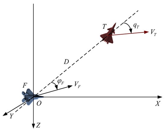
Figure 1. Dual-aircraft geometric situation map.

When conducting a threat assessment of a target, it is necessary to comprehensively consider numerous factors [14]. It is necessary not only to consider the enemy’s and our situation and the performance of the weapons carried in the confrontation but also to consider the air environment at that time, whether there is electromagnetic interference, and other factors. Therefore, threat assessment of airborne targets is a complex, nonlinear, multi-attribute decision-making problem [15]. In this study, the speed, angle, altitude, distance, and operational capability threats were selected to quantify the threat level of the target.

(1) Speed threat

$$T_V=\left\{\begin{array}{l}0.1,V_T<0.6V_F\\ -0.5+V_T/V_F,0.6V_F\le V_T\le 1.5V_F\\ 1.0,V_T>1.5V_F\end{array}\right.$$

(1)

(2) Angle threat

$$T_A={\displaystyle \frac{(\left|{\phi }_F\right|+\left|q_T\right|)}{{360}^{\circ }}}$$

(2)

(3) Altitude threat

$$T_H=\left\{\begin{array}{l}1.0,H\ge 5000\\ 0.5+0.0001H,-5000\le H\le 5000\\ 0.1,H<-5000\end{array}\right.$$

(3)

(4) Distance threat

The effect of the distance factor on the target threat is mainly reflected in the probability of the airborne radar detecting the target and the probability of the airborne weapon killing the target. These probabilities decrease as the distance between the enemy aircraft and the aircraft increases. Therefore, distance $D$ between the enemy and us is divided into the maximum detection distance $D_{R\max }$ of the airborne radar, the boundary distances $D_{MA\max }$ and $D_{MA\min }$ of the missile’s attack zone, and the inescapable distances $D_{ME\max }$ and $D_{ME\min }$ in order to establish the distance threat function.

$$T_D=\left\{\begin{array}{l}0,D\ge D_{R\max }\\ 0.5e^{-{\displaystyle \frac{D-D_{MA\max }}{D_{MA\max }-D_{R\max }}}},D_{MA\max }\le D<D_{R\max }\\ 2^{-{\displaystyle \frac{D-D_{ME\max }}{D_{MA\max }-D_{ME\max }}}},D_{ME\max }\le D<D_{MA\max }\\ 1,D_{ME\min }\le D<D_{ME\max }\end{array}\right.$$

(4)

(5) Operational capability threat

According to [16], the operational capability of an aircraft is determined by seven parameters: maneuverability, airborne weapon performance, airborne detection capability, operational performance, aircraft survivability, range, and electronic information countermeasure capability. The calculation expression is as follows:

$$C=[\ln {\epsilon }_1+\ln ({\epsilon }_2+1)+\ln ({\displaystyle \sum {\epsilon }_3}+1)]{\epsilon }_4{\epsilon }_5{\epsilon }_6{\epsilon }_7$$

(5)

where ${\epsilon }_1\sim {\epsilon }_7$ represents seven parameters: maneuverability, airborne weapon performance, airborne detection capability, operational performance, aircraft survivability, range, and electronic information countermeasure capability.

Based on Equation (5), to calculate the operational capability of a fighter aircraft, the threat function of the fighter aircraft’s operational capability can be obtained as follows:

$$T_C=\left\{\begin{array}{l}{\displaystyle \frac{1}{2}}{e}^{1-{\displaystyle \frac{C_T}{C_F}}},C_T\le C_F<40\\ {\displaystyle \frac{1}{2}}+{\displaystyle \frac{1}{2(e-1)}}(e^{2-{\displaystyle \frac{2C_T}{C_F}}}-1),40>C_T>C_F\end{array}\right.$$

(6)

where $C_F$ is the operational capability of our aircraft and $C_T$ is the operational capability of the enemy aircraft.

(6) Composite threat index

$$E=w_1{T}_V+w_2{T}_A+w_3{T}_H+w_4{T}_D+w_5{T}_C$$

(7)

where $w_i(i=1,2,\cdots ,5)$ denotes the weight of each threat assessment index. Each weight was determined using the expert scoring method; however, this method is highly subjective, and its accuracy is closely related to the experience of the selected experts. To process operational information more objectively, this study uses [17] to improve the rough set theory to determine the weight of the index.

2.2. Multi-Aircraft Coordinated Comprehensive Situational Advantage Assessment Model

Assume we have an $\mathit{m}$ aircraft and the enemy has an $\mathit{n}$ aircraft. Based on the single-target threat assessment model constructed in the previous section, we can establish the advantage matrix $\mathit{S}$ of our aircraft over the enemy aircraft and the threat matrix $\mathit{T}$ of the enemy aircraft against our aircraft:

$$\mathit{S}=\left[\begin{array}{cccc}{S}_{11}& S_{12}& \cdots & S_{1n}\\ S_{21}& S_{22}& \cdots & S_{2n}\\ ⋮& ⋮& \ddots & ⋮\\ S_{m1}& S_{m2}& \cdots & S_{mn}\end{array}\right]$$

(8)

$$\mathit{T}=\left[\begin{array}{cccc}{T}_{11}& T_{12}& \cdots & T_{1n}\\ T_{21}& T_{22}& \cdots & T_{2n}\\ ⋮& ⋮& & ⋮\\ T_{m1}& T_{m2}& \cdots & T_{mn}\end{array}\right]$$

(9)

where $S_{ij}$ is the situational advantage of our aircraft $i$ over the enemy aircraft $j$ and $T_{ij}$ is the threat value of the enemy aircraft $j$ to our aircraft $i$.

Based on the threat matrix of the enemy aircraft against our aircraft and the importance of the enemy aircraft $j$, importance ${\alpha }_j$ can be obtained and satisfies ${\displaystyle \sum _{j=1}^n{\alpha }_j}=1$.

$${\alpha }_j={\displaystyle \frac{{\displaystyle \sum _{i=1}^m{T}_{ij}}}{{\displaystyle \sum _{i=1,j=1}^{i=m,j=n}{T}_{ij}}}}$$

(10)

Through an analysis of the classic advantage function, it can be observed that the function does not fully consider the coordination relationship between our aircraft. Therefore, with the help of relevant knowledge of probability theory, our aircraft $i$ confronts the enemy aircraft $j$ with situational advantage $S_{ij}$, which is used as the probability of shooting down the enemy aircraft, to build a comprehensive advantage function of multi-aircraft coordination.

2.2.1. The Situation of Many to One

As shown in Figure 2, our $m$ aircraft confronted a single enemy aircraft. Our comprehensive situational advantages are as follows:

$$S_{m1}=1-{\displaystyle \prod _{i=1}^m(1-S_{i1})}$$

(11)

Figure 2. Schematic diagram of multiple aircraft confronting a single-target aircraft.

2.2.2. The Situation of Many to Many

As shown in Figure 3, when our $m$ model combines aircraft to confront $n$ enemy aircraft, there are two scenarios for calculating the comprehensive situational advantage. The main factor to consider is whether coordination exists between our $m$ aircraft or not.

Figure 3. Schematic diagram of our multiple aircraft confronting multiple target aircraft.

(1) Lack of coordination among multiple aircraft

When there is lack of coordination among multiple aircraft, we assume that our $k_i({\displaystyle \sum _{i=1}^n{k}_i}=m)$ aircraft encounter the target $i$. Then, our comprehensive advantage function in the multi-aircraft lack of coordination is the following:

$$\begin{array}{l}S(G)={\displaystyle \sum _{i=1}^n{\alpha }_i{S}_{k_{i}i}}\cdot {\displaystyle \prod _{j=1}^{i-1}(1-S_{k_{j}j})}\cdot {\displaystyle \prod _{j=i+1}^n(1-S_{k_{j}j})}+{\displaystyle \sum _{i=1,j=2,i\ne j}^{i=n-1,j=n}({\alpha }_i+{\alpha }_j)S_{k_{i}i}}\cdot S_{k_{j}j}\cdot {\displaystyle \prod _{m=1}^{i-1}(1-S_{k_{m}m})}\cdot {\displaystyle \prod _{m=i+1}^{j-1}(1-S_{k_{m}m})}\cdot \\ {\displaystyle \hspace{1em}\hspace{1em}\prod _{m=j+1}^n(1-S_{k_{m}m})}+\cdots +{\displaystyle \sum _{i=1}^n\left({\displaystyle \sum _{k=1,k\ne i}^n{\alpha }_k}\right)}\cdot S_{k_{1}1}\cdot S_{k_{2}2}\cdots (1-S_{k_{i}i})\cdots S_{k_{n}n}+S_{k_{1}1}\cdot S_{k_{2}2}\cdots S_{k_{n}n}\end{array}$$

(12)

where $S_{k_{i}i}$ is the situational advantage of our aircraft $k_i$ over the enemy aircraft $i$.

(2) Coordination among multiple aircraft

In the event that we have multiple aircraft coordination, our comprehensive situational advantage is as follows:

$$S_{Xi}=1-{\displaystyle \prod _{m=1}^n(1-S_{k_{m}i})}$$

(13)

$S_{Xi}$ substitutes for $S_{k_{i}i}$ in Equation (12), and the comprehensive situation $S^{\prime }(G)$ in multi-aircraft coordination can be obtained. Similarly, the comprehensive threat $T^{\prime }(G)$ posed by a coordinated enemy aircraft against our aircraft can be obtained.

2.3. Multi-Aircraft Coordinated Target Assignment Model

2.3.1. Target Assignment Model

In the study of the target assignment problem, the following three modes were identified based on the quantitative relationship between our aircraft and the enemy aircraft:

(1) Mode 1: In the case of $m=n$, i.e., when the number of enemy aircraft is equal to that of our aircraft, the target assignment problem is quite simple if each of our aircraft can be matched against only one target. In this case, the algorithm complexity is the lowest, and the key element in the algorithmic optimization process is to avoid conflicts caused by the target competition.

(2) Mode 2: In the case of $m>n$, i.e., when the number of targets is less than that of our aircraft, each target may be assigned to one or more of our aircraft, and each of our aircraft must be assigned to a target. There is a many-to-one relationship between our aircraft and the targets, and there is an imbalance in the relationship between the targets and our aircraft, which leads to higher algorithm complexity. A fundamental challenge in target assignment is the formulation and satisfaction of resource quantity constraints to achieve optimal assignment.

(3) Mode 3: In the case of $m<n$, i.e., the number of targets is greater than the number of aircraft, there is a one-to-many relationship between our aircraft and the targets. The target assignment problem is the most complex, and the key to the problem is to obtain the maximum comprehensive advantage function value of the target assignment.

2.3.2. Unified Modeling for Multi-Aircraft Coordinated Target Assignment Mode

Multi-aircraft coordinated target assignment is essentially the same as the task assignment problem in operational research. Assume that we have an m aircraft and the enemy has an n aircraft. The constructed objective function must meet the quantity constraint relationship between the enemy aircraft and our aircraft, be in line with operational reality, and uniformly process the target assignment problem in three different modes. Based on this, the objective function was established as follows:

$$\max f=alloc(m,n)\cdot (\alpha \cdot S^{\prime }(G)+(1-\alpha )\cdot (1-T^{\prime }(G))-\beta \cdot pe)$$

(14)

where $\max f$ is the comprehensive evaluation function representing the optimal decision outcome. Its quantification method integrates assessments across three dimensions—tactical advantages, enemy threats, and solution feasibility—into a single scalar value through weighted summation and a penalty mechanism; $\alpha$ is the importance degree coefficient of the operational situation and satisfies $\alpha \in [0,1]$; the greater the $\alpha$ value is, the more important the situational advantage of our aircraft and the more adventurous our decision-making; the smaller the $\alpha$ value is, the more important the threat of enemy aircraft against our aircraft and the more conservative our decision-making; $pe$ is the penalty term corresponding to the constraint; $\beta$ is the penalty term contraction coefficient; $alloc(m,n)$ is the decision matrix:

$$alloc(m,n)={[d(i,j)]}_{m\times n}$$

(15)

where $d(i,j)$ is a decision variable with values 0 and 1. This parameter determines the matching relationship between our fighter and the targets and is defined as follows for the three modes:

$$d(i,j)=\left\{\begin{array}{l}\begin{array}{cc}d(i,j)& m=n\end{array}\\ \begin{array}{cc}d([i_s,\cdots ,i_l],j)& s,l\in m m>n\end{array}\\ \begin{array}{cc}d(i,[j_p,\cdots ,j_q])& \forall p,q\in n m<n\end{array}\end{array}\right.$$

(16)

In the above equation, when the number of enemy aircraft and that of our aircraft satisfy $m=n$, $d(i,j)$ means that there is a one-to-one correspondence between our aircrafts and the targets, that is, the number of enemy aircraft confronted by our aircraft is $m>n$; $d([i_s,\cdots ,i_l],j)$ means that there is a many-to-one correspondence between our aircraft and the targets, that is, target $j$ is confronted by our aircraft $[i_s,\cdots ,i_l]$. To guarantee the effectiveness of the confrontation, this study restricted the number of aircraft that confronted the target. When the number of enemy aircraft and that of our aircraft satisfy $m<n$, $d(i,[j_p,\cdots ,j_q])$ means that there is a one-to-many correspondence between our aircraft and the targets, that is, target $[j_p,\cdots ,j_q]$ is confronted by our aircraft $i$. In this mode, considering the multitarget operational capability of the aircraft and the limitation of the number of airborne weapons to ensure that each aircraft can be assigned to a target, this study restricts the number of targets to be confronted by our aircraft.

2.3.3. Constraint Processing

Common methods for solving optimization problems with constraints include the gradient descent and barrier function methods. The simplest and most common method for solving the constraint problem is the penalty function method. Based on constructive thinking, this method converts a constrained optimization problem into an unconstrained optimization problem.

In the multi-aircraft coordinated target assignment optimization problem, what needs to be dealt with is the constraint of the decision variable between our aircraft and the targets: when the number of enemy aircraft and that of our aircraft satisfy $m\ge n$, the decision constraint is that each of our aircraft must confront one target and each target must be confronted by one aircraft; when the number of enemy aircraft and that of our aircraft satisfy $m<n$, the decision constraint is that each target must be assigned to one of our aircraft. The feasible solution domain $L$ for multi-aircraft coordinated target assignment is as follows:

$$m=n\left\{\begin{array}{l}\begin{array}{cc}{\displaystyle \underset{j=1}{\overset{n}{\cap }}d(i,j)=1,}& \forall i=1,\cdots ,m\end{array}\\ \begin{array}{cc}{\displaystyle \underset{i=1}{\overset{m}{\cap }}d(i,j)=1,}& \forall j=1,\cdots ,n\end{array}\end{array}\right.$$

(17)

$$m>n\left\{\begin{array}{l}\begin{array}{cc}{\displaystyle \underset{j=1}{\overset{n}{\cap }}d(i,j)=1,}& \forall i=1,\cdots ,m\end{array}\\ \begin{array}{cc}1\le {\displaystyle \underset{i=1}{\overset{m}{\cap }}d(i,j)\le 2,}& \forall j=1,\cdots ,n\end{array}\end{array}\right.$$

(18)

$$m<n\left\{\begin{array}{l}\begin{array}{cc}{\displaystyle \underset{i=1}{\overset{m}{\cap }}d(i,j)=1,}& \forall i=1,\cdots ,m\end{array}\\ \begin{array}{cc}1\le {\displaystyle \underset{j=1}{\overset{n}{\cap }}d(i,j)\le 2,}& \forall j=1,\cdots ,n\end{array}\end{array}\right.$$

(19)

Equations (17)–(19) represent the constraint relationships of the decision variables in the three modes. Based on the constraints of the decision variables, the value of the penalty term can be determined using the quation as follows:

$$pe(z)=\left\{\begin{array}{l}\begin{array}{cc}0\hfill & z\notin D\end{array}\\ \begin{array}{cc}1\hfill & z\in D\end{array}\end{array}\right.$$

(20)

where $z$ is an optimization variable.

3. Salp Swarm Algorithm

The SSA [18] is a new heuristic swarm intelligence optimization algorithm proposed by Mirjalili et al. based on the assembly behavior of salps. The core idea of the algorithm is to create a salp chain by simulating the assembly behavior of a salp. There are two types of salp in the salp chain: leaders and followers. The leader is the salp head, and all the salps behind it in the chain are followers. The salp chain is illustrated in Figure 4.

Figure 4. Structure of a salp chain.

Assuming that the search space dimension of the problem to be optimized is $R$, each salp individual in the salp chain represents a position vector $(x_1,x_2,\cdots ,x_R)$, and the salp chain composed of salp individuals can be regarded as a population. The salp population vector can then be represented by a matrix of $R\times d$ dimensions:

$$X_i=\left[\begin{array}{cccc}{x}_1^1& x_2^1& \cdots & x_d^1\\ x_1^2& x_2^2& \cdots & x_d^2\\ ⋮& ⋮& \ddots & ⋮\\ x_1^R& x_2^R& \cdots & x_d^R\end{array}\right]$$

(21)

In the salp population, the objective of all salps is to determine the location of food. Therefore, in the evolved salp swarm algorithm, the optimal solution to the problem to be optimized is equivalent to determining the food location. The leader and followers in the salp chain abide by the different rules for position updating. The position-updating formula for the leader is as follows:

$$x_j^1=\left\{\begin{array}{l}{F}_j+c_1((ma{x}_j-mi{n}_j)c_2+mi{n}_j),c_3\ge 0.5\\ F_j-c_1((ma{x}_j-mi{n}_j)c_2+mi{n}_j),c_3<0.5\end{array}\right.$$

(22)

where $x_j^1$ is the $j$ dimension component of the location of the salp leader, $F_j$ is the $j$ dimension component of the location of food, $ma{x}_j$ is the maximum value of the $j$ dimension search space, $mi{n}_j$ is the minimum value of the $j$ dimension search space, and $c_2$ and $c_3$ are random numbers with the value of $[0,1]$. $c_2$ determines the length of each iteration movement of the salp, $c_3$ determines the direction of each iteration movement, and $c_1$ is the parameter that controls the search capability and development capability of all salp individuals in the population and is related to the algorithm’s number of iterations:

$$c_1=2e^{-{({\displaystyle \frac{4t}{T\max }})}^2}$$

(23)

where $t$ is the current number of iterations of the algorithm and $T_{\max }$ is the maximum number of iterations.

Followers of the salp population move by following their leaders. For the $i$ follower salp, the position change in the next iteration is determined by the position of the salp in the current iteration and that of the $i-1$ follower salp. According to Newton’s law of kinematics, we can obtain the following formula for updating the positions of the followers in the salp chain:

$$x_j^i={\displaystyle \frac{1}{2}}a{t}^2+v_0\Delta t$$

(24)

$$a=(v_{final}-v_0)/\Delta t$$

(25)

$$v_{final}=(x_j^{i-1}-x_j^i)/\Delta t$$

(26)

where $x_j^i$ is the $i$ follower salp’s $j$ dimension position component; $\Delta t$ is the time difference; $v_0$ is the initial velocity of the follower salp; and $x_j^{i-1}$ is the $i-1$ follower salp’s $j$ dimension position component. In this algorithm, the time difference is the difference between the two numbers of iterations; therefore, it is $\Delta t=1$ and the initial velocity is $v_0=0$. Based on this, the follower’s position-updating formula can be rewritten as follows:

$$x_j^i={\displaystyle \frac{1}{2}}(x_j^i+x_j^{i-1})$$

(27)

By using Equations (22) and (27), a salp chain is formed. Based on the above analysis, the pseudocode of the SSA is presented in Algorithm 1.

Algorithm 1: Salp swarm algorithm

1. Initialize the randomly generated population of the salp swarm $X_i(i=1,2,\cdots ,r)$. 2. Calculate the fitness values of each salp. 3. $X^{*}=the best search agent$ 4. while stopping criteria not reached 5. Update $c_1$ by (23) 6. for each salp 7.  if $(r==1)$ 8.    Update the position of the leader salp by (22) 9.  else 10.    Update the position of the follower salp by (22) 11.  end if 12. end for 13. Calculate the fitness values of every salp. 14. Update $X^{*}$ if there is a better solution. 15. end while 16. return the best solution $X^{*}$ and its fitness value.

4. Adaptive Salp Swarm Algorithm Based on Chaotic Mutation (CMASSA)

4.1. Chaotic Search Strategy with Contraction Mechanism

Chaos [19] is essentially a nonlinear phenomenon characterized by non-periodicity, ergodicity, randomness, and sensitivity to the initial conditions. Chaos is similar to random behavior and has a certain regularity. Chaos can traverse all states in space without repetition within a certain scope range according to their regularity. Given the chaotic properties of chaos, its introduction into the salp swarm algorithm can effectively prevent it from falling into locally optimal solutions. Compared with the random search method, searching the solution space using chaotic variables is more conducive to improving search and development capabilities. Many chaotic models are commonly used, and a logistic mapping model is typically used. Introducing a logistic mapping model into the SSA can effectively improve its performance. The chaotic sequence obtained using the logistic mapping model is as follows:

$$C_{i+1}=\tau C_i(1-C_i)i\in \{1,2,\cdots ,R\}$$

(28)

where $\tau$ denotes the chaotic adjustment coefficient. When its value is $\tau =4$, the logistic mapping model exhibits chaotic characteristics. Therefore, in this study, $\tau =4$ is used, where $C_1$ is a random number and $C_1\in [0,1] \& C_1\ne 0,$$0.25, 0.50, 0.75, 1.00$. Using $\tau =4$, $C_1=0.4501$ denotes the initial mapping value. After 10,000 iterations of the logistic mapping and the random mapping, the distribution of the chaotic sequences in the two-dimensional space is shown in Figure 5 and Figure 6.

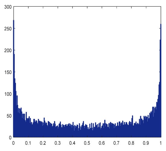
Figure 5. Logistic mapping distribution.

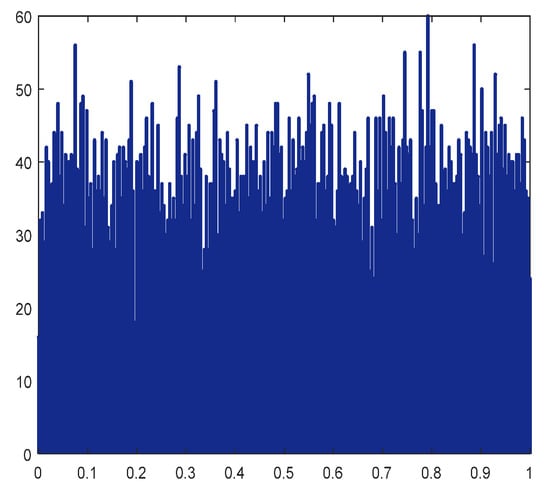
Figure 6. Stochastic mapping distribution.

Figure 5 and Figure 6 clearly indicate that logistic mapping has a greater probability of taking values at both ends and a uniform probability of taking values in the middle, whereas random mapping is more uniformly distributed than logistic mapping. When the search space of the algorithm is small, the modified algorithm based on chaotic mutation has a good optimization effect, which can improve the search and development capabilities of the algorithm and effectively prevent it from falling into a local optimum. The specific implementation steps of the chaotic local search strategy with the contraction mechanism are as follows:

Step 1: Use Equation (29) to map the chaotic variable $C_i$ generated using Equation (28) into the chaotic vector’s $C{H}_i$ search range: $[lb,ub]$

$$C{H}_i=lb+C_i(ub-lb)i=1,2,\cdots ,R$$

(29)

Step 2: Use Equation (30) for the linear weighting of the chaotic vector and the current optimal position of the salp to obtain the optimal alternate position:

$$V_i=(1-\lambda )\times FoodPosition+\lambda \times C{H}_i$$

(30)

where $FoodPosition$ is the current optimal position of the algorithm and $\lambda$ is the contraction control parameter, which is determined by the following formula:

$$\lambda =1-{\left|{\displaystyle \frac{t-1}{t}}\right|}^b$$

(31)

where $t$ is the current number of iterations of the algorithm and $b$ controls the contraction rate. The contraction rate decreases as $b$ increases. According to Equation (31), the contraction rate was set to $b=1000$ in this study. The variation process of the contraction control parameter $\lambda$ over 1000 algorithmic iterations is shown in Figure 7.

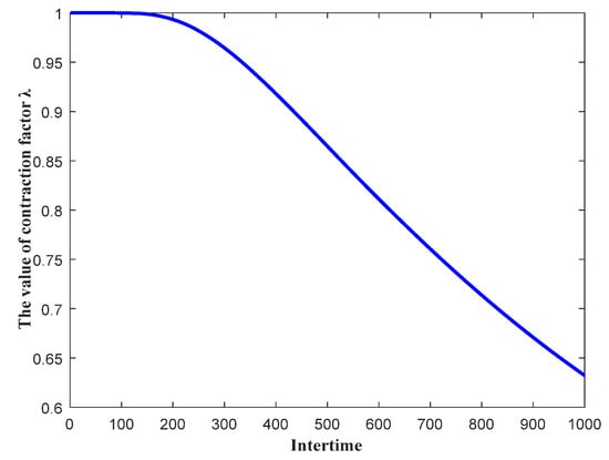
Figure 7. Convergence trend of contraction control parameter $\lambda$.

As shown in Figure 7, $\lambda$ continued to decrease as the number of iterations of the algorithm increased. According to Equation (30), it can be observed that, as the contraction control parameter $\lambda$ continues to decrease, the corresponding chaotic search range continues to decrease. In addition, as can be seen from the convergence curve in Figure 7, the contraction control parameter $\lambda$ is relatively large in the early stages of the iteration of the algorithm, which is conducive to expanding the search range of the algorithm. In the late stage of the iteration of the algorithm, $\lambda$ gradually decreases, which is conducive to the algorithm avoiding falling into the locally optimal solution and allows the algorithm to further approach the globally optimal solution.

4.2. Combined Mutation Strategy

To improve the performance of the salp swarm algorithm, it is necessary to improve its global and local search capabilities simultaneously. However, it is difficult to satisfy these requirements by using a single-mutation strategy. Therefore, by analyzing the two operators, including Gaussian and Cauchy mutations, this study effectively uses two mutation operators to provide a mutation operation with both strong global search capability and good local search capability.

4.2.1. Gaussian Mutation

A Gaussian distribution is a probability distribution that is also known as normal distribution. It can accurately describe random behaviors and events, and its probability density function is given by the following equation:

$$f(x)={\displaystyle \frac{1}{\sqrt{2\pi }\sigma }}exp\left(-{\displaystyle \frac{{(x-\mu )}^2}{2{\sigma }^2}}\right)$$

(32)

where $\mu$ is the mean value and $\sigma$ is the variance.

A Gaussian mutation superposes a random vector obeying a Gaussian distribution on the position vector of the original salp individual. Previous studies have indicated that the introduction of Gaussian mutations into heuristic intelligent algorithms such as BSO [20] and PSO [21] can improve the overall performance of these algorithms. In the salp swarm algorithm, a Gaussian mutation is used to mutate the positions of salp individuals. This is defined as follows:

$$mut\_SalpPositions\_G=SalpPositions\times (1+N(0,1))$$

(33)

where $N(0,1)$ denotes the standard Gaussian distribution. Equation (33) adds a stochastic disturbance, $SalpPositions\times N(0,1)$, that obeys a Gaussian distribution to the original position of the salp individuals. Thus, by adequately using the positional information disturbance of the current population, we can free salp individuals from the constraint of the local extremum point and obtain a global optimum. In addition, Gaussian chaotic mutation improved the convergence rate of the algorithm.

4.2.2. Cauchy Mutation

The Cauchy distribution is a special continuous distribution with many unique features. The one-dimensional Cauchy distribution probability density function is given in the following equation:

$$f(x,\delta ,\mu )={\displaystyle \frac{1}{\pi }}{\displaystyle \frac{\delta }{{\delta }^2+{(x-\mu )}^2}},-\infty <x<\infty$$

(34)

When $\delta =1,\mu =0$ is satisfied, the distribution is the standard Cauchy distribution, which can be expressed as follows:

$$f(x)={\displaystyle \frac{1}{\pi }}{\displaystyle \frac{1}{x^2+1}},-\infty <x<\infty$$

(35)

The standard Cauchy distribution function is given in the following equation:

$$Cauchy(0,1)=\tan [(\xi -0.5)\pi ],\xi \in U[0,1]$$

(36)

The Cauchy mutation has been applied in other heuristic intelligent optimization algorithms, such as the grasshopper optimization algorithm (GOA) [22] and the genetic algorithm (GA) [23]. In this study, we used the Cauchy mutation to randomly disturb the position of the salp individuals to improve the diversity of the population, thus preventing the algorithm from falling into a locally optimal solution and improving the optimization performance of the salp swarm algorithm. The Cauchy mutation is expressed as follows:

$$mut\_SalpPositions\_C=SalpPositions\times (1+Cauchy(0,1))$$

(37)

4.2.3. Combined Mutation

The Gaussian and Cauchy distribution curves are shown in Figure 8. As shown in the figure, the middle region of the Cauchy distribution curve is lower than that of the Gaussian distribution curve, whereas the regions on both sides are higher than those of the Gaussian distribution curve. The two flanks are narrow, which is a characteristic of a typical two-flank probability distribution. This indicates that the Cauchy distribution can generate random numbers with a high probability; that is, the Cauchy distribution can generate a large algorithmic change step size with a high probability. From the above analysis, it can be seen that the Gaussian mutation has good development capability and can accelerate the convergence rate of the algorithm. The Cauchy mutation has good search capability and prevents the algorithm from falling into a locally optimal solution. It can guide the algorithm to overcome the limitation of the locally optimal solution to prevent the algorithm from falling into a locally optimal solution.

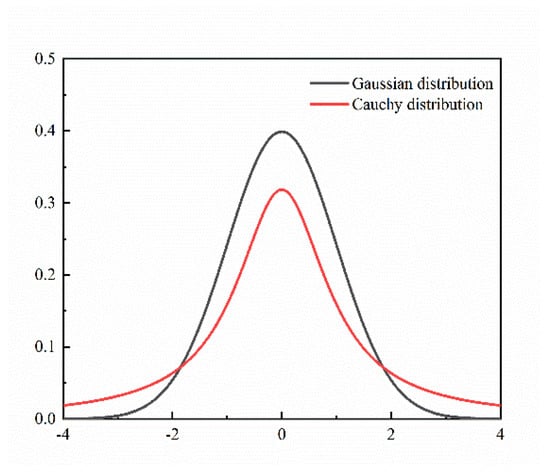
Figure 8. Comparison of Gaussian and Cauchy distribution probability density curves.

After analyzing the performance of the Gaussian and Cauchy mutations, we found that both mutations have their respective advantages. Therefore, Gaussian and Cauchy mutations were combined in Algorithm 2.

Algorithm 2: Combined mutation

for (each individual $i(i=1,2,\cdots ,R)$)   $temp=R-i$ Step 1 is described as follows: /*Execute the cycle $(R-i)$ times*/ for $ant=1:temp$ /*After the current salp individual $i$, execute combined mutation of the positions $SalpPositions(antk,:)$ of all salp individuals*/   $antk=ant+i;$ /*Execute Gaussian mutation of the salp individuals by using Equation (33) to obtain */ $mut\_SalpPositions\_G(ant,:)=SalpPositions(antk,:)\ast (1+N(0,1))$ /*Calculate the function fitness corresponding to the salp $mut\_SalpPositions\_G(ant,:)$*/ $mut\_fit\_G(ant)=fobj(mut\_SalpPositions\_G(ant,:));$ /*Execute Cauchy mutation of the salp individuals by using Equation (37) to obtain */ $mut\_SalpPositions\_C(ant,:)=SalpPositions(antk,:)\ast (1+Cauchy(0,1))$ /*Calculate the function fitness corresponding to the salp  $mut\_SalpPositions\_G(ant,:)$*/ $mut\_fit\_C(ant)=fobj(mut\_SalpPositions\_C(ant,:));$ /*After the current salp individual $i$, record the positions $SalpPositionsAnt(ant,:)$ of all salp individuals */ $SalpPositionsAnt(ant,:)=SalpPositions(ant,:)\_$ /*Calculate the function fitness corresponding to the salp $SalpPositionsAnt(ant,:)$*/ $mut\_fit\_my(ant)=fobj(SalpPositionsAnt(ant,:));\_$ end end Step 2 is described as follows: /*Combine the aforesaid three different individuals and fitness degrees described and record them as $AllSalPositions$ and $AllFitness$, respectively*/ $Allsalpositions=[mut\_SalpPositions\_G;mut\_SalpPositions\_C;SalpPositionsAnt]\_$  $AllFitness=[Mut\_fit\_G;Mut\_fit\_C;Mut\_fit\_my]\_$ /*Sort the function fitness degrees $AllFitness$ in ascending order*/ $[AllFitness\_temp,Index]=sort(AllFitness);$ /*Store $AllSalPositions$ in $AllSalPositions\_tmp$*/ $AllSalPositions\_tmp=AllSalPositions$ /*Based on the function fitness degrees $AllFitness$ sorted in ascending order, reorder $AllSalPositions$*/ for $ij=1:size(AllSalPositions,1)$  $\hspace{1em} AllSalPositions(ij,:)=AllSalPositions\_tmp(Index(ij),:);$ end /*From $AllSalPositions$, select the $temp$ optimal individual and find the corresponding fitness value*/ $AllSalPositionsTemp=AllSalPositions(1:temp,:);$/*Use $AllSalPositionsTemp$ to update the position $SalPositions$ of the salp individuals after the current individual $i$*/ for $jj=1:temp$  $\hspace{1em}jjTemp=jj+i;$  $\hspace{1em}SalPositions(jjTemp,:)=SalPositionsTemp(jj,:);$ end end

4.3. Adaptive Inertia Weight Strategy

The adaptive inertia weight $\omega$ is introduced into the salp swarm algorithm and embodies the ability of the follower to follow the position of the previous salp individual. When the inertia weight value is large, the search capability of the algorithm improves. When the inertia weight is small, it improves the development capability of the algorithm. From the follower position-updating Formula (27) in the salp swarm algorithm, it can be observed that the $i$ salp individual is updated based on its current position and the position of the $i-1$ salp individual and that there is a strong correlation between the historical positions of the individuals. If the follower falls into a locally optimal solution, the algorithm is likely to fall into a locally optimal solution, and stagnation occurs. To better balance the search and development capabilities of the salp swarm algorithm, an adaptive inertia weight is introduced into the salp swarm algorithm, which helps the algorithm avoid falling into a locally optimal solution. The follower position-updating formula based on the adaptive inertia weight is given by the following equation:

$$x_j^i={\displaystyle \frac{1}{2}}(x_j^i+\omega (t)x_j^{i-1})$$

(38)

$$\omega (t)={\omega }_s({\omega }_s-{\omega }_e)(T_{\max }-t)/T_{\max }$$

(39)

where ${\omega }_s$ denotes the initial weight of the algorithm and ${\omega }_e$ denotes the inertial weight at the end of the algorithm. In this study, the parameter was set as ${\omega }_s=0.9,{\omega }_e=0.4$. As the algorithm iteration proceeds, the inertia weight adaptively decreases from 0.9 to 0.4. At the beginning of the search, a large inertia weight provides the algorithm with good search capability, whereas in the later stage, a small inertia weight improves the algorithm’s development capability.

4.4. CMASSA Steps

In summary, three strategies were introduced to improve the performance of the salp swarm algorithm, and a modified CMASSA was proposed. First, a chaotic search strategy with a contraction mechanism was applied to the basic SSA, thus enhancing the search capability of the algorithm. Then, by analyzing the respective advantages of the Gaussian and Cauchy mutations, the combined mutation of the Gaussian and Cauchy mutations was embedded into the SSA to enhance the development and search capabilities of the algorithm in the optimization process. Finally, to balance the search and development capabilities of the algorithm, an adaptive inertia weight was introduced to improve the position-updating rule of the follower salp and avoid the problem of imbalance between the search and development capabilities of the algorithm. The steps of the modified SSA based on the above three strategies are presented in Algorithm 3.

Algorithm 3: CMASSA pseudocode

Initialize the positions $SalpPosition{s}_i(i=1,2,\cdots ,R)$ of all individuals in the salp population. Calculate the initial function fitness of each salp individual. The fitness values of all individuals in the salp population are sorted, the position of the best individual is recorded as $FoodPosition$, and the function fitness value corresponding to it is recorded as $FoodPosition$ While $(t<T_{\max })$   for $i=1:R$ if $(i<R/2)$ then Update the position of the leader according to Equation (22) else Update the position of the follower according to Equation (27) end Use Equation (30) to execute the chaotic search strategy with the contraction mechanism to generate candidate individual position $V_i$; calculate the fitness of the candidate position $V_i$, and record it as $FitnessV$ if $(FitnessV<FoodFitness)$ then Update the optimal position $FoodPosition$ and its fitness value $FoodPosition$ end Execute the combined mutation step in Algorithm 2 end Output the optimal position $FoodPosition$ and its fitness value $FoodPosition$

4.5. Complexity of the CMASSA

The complexity of the basic SSA and modified CMASSA depends on the number of iterations (t) of the algorithm and number of salp individuals (r). The complexity of the basic salp swarm algorithm includes salp initialization, calculation of the initialized salp individual fitness, selection of optimal individuals, updating of salp individual positions in the algorithm iteration, and calculation of fitness. The complexity of the modified CMASSA algorithm includes salp initialization, calculation of the initialized salp individual fitness, selection of optimal individuals, updating of salp individual positions in the algorithm iteration, calculation of fitness, execution of a chaotic search with a contraction mechanism, combined mutation, adaptive inertia weight, and fitness calculation. The time complexity of each algorithm is presented in Table 1.

Table 1. Time complexity of each operation.

Operation	Time Complexity
Initialization	$O(r)$
Calculate initialized individual fitness	$O(r)$
Select the optimal individual	$O(r)$
Update the position of individual	$O(r)$
Calculate the fitness of updated individual	$O(r)$
Execute the chaotic search with contraction mechanism	$O(r^2)$
Execute combined mutation	$O(r^2)$
Identify the best individual from combined mutation	$O(r^2)$
Update the position of salp individuals after execution of the optimization strategy and calculate the fitness	$O(r^2)$
Execute adaptive inertia weight	$O(1)$

Based on the theoretical analysis of the SSA and modified CMASSA algorithms and considering the time complexity of each operation in Table 1, the time complexity of the SSA and CMASSA algorithms can be obtained as follows:

$$O(SSA)=O(r)+O(r)+O(r)+t\times (O(r)+O(r))=3O(r)+t\times 2O(r)$$

(40)

$$\begin{array}{l}O(CMASSA)=O(r)+O(r)+O(r)+t\times (O(r)+O(r^2)+O(r^2)+O(r^2)+O(r^2)+O(1))\\ \hspace{1em}\hspace{1em}\hspace{1em}=3O(r)+t\times (O(r)+4O(r^2)+O(1))\end{array}$$

(41)

A comparison of the time complexities of the above algorithms indicates that the modified CMASSA has higher time complexity than the basic SSA.

5. Multi-Aircraft Coordinated Target Assignment Model Based on CMASSA

To prevent the algorithm from falling into a local optimum and improve the convergence accuracy of the algorithm, this study introduces a chaotic search strategy with a contraction mechanism, a combined mutation strategy based on Gaussian and Cauchy mutations, and the modified salp swarm algorithm of the adaptive inertia weight strategy. The multi-aircraft coordinated target assignment process using this algorithm is illustrated in Figure 9.

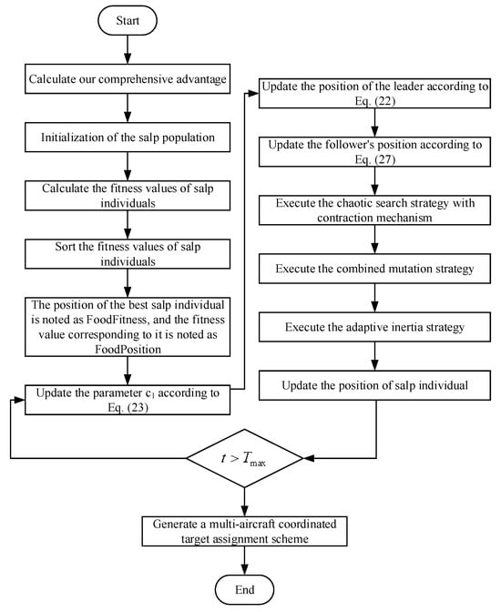
Figure 9. Flowchart of target assignment.

As shown in Figure 9, the target assignment steps of the modified CMASSA algorithm are as follows:

Step 1: Calculate the threat and situational advantage of the enemy aircraft against us, obtain our comprehensive advantage matrix, and initialize the salp population. The assignment scheme with the greatest comprehensive advantage was used as the initial target assignment scheme, which was coded using the integer coding method. Equation (14) represents the fitness function of the algorithm.

Step 2: To address the deficiencies of the salp swarm algorithm, SSA is improved using a chaotic search with a contraction mechanism, a combined mutation strategy, and an adaptive inertia weight strategy.

Step 3: Determine the termination condition of the algorithm. We determine whether the algorithm satisfies the termination condition. If so, proceed to the next step. Otherwise, return to step 2.

Step 4: Generate the final multi-aircraft coordinated target assignment scheme, and output the optimal target assignment result.

6. Simulation Analysis

6.1. Validate the Effectiveness of the Target Assignment Model Based on the Modified Salp Swarm Algorithm

6.1.1. Static Target Assignment in Different Modes

There are some equations and inequality constraints in most target assignment problems. These constraints must first be addressed to solve these problems. The search process of CMASSA is independent of the function fitness value; therefore, the algorithm can solve the constraints of the target assignment during the optimization process without changing its mechanism. In the CMASSA algorithm, the simplest method for constraint handling is selected, which is the penalty function [24]; this implies that a poor objective function value is assigned to a salp individual when it violates any constraint during the search process. This process automatically causes an infeasible solution to be discarded during the optimization of the heuristic algorithm. The most striking advantages of this method are its simplicity and low costs.

The maximum number of evolutionary generations of the algorithm was set to 200, and the adaptive inertia weight, chaotic search with a contraction mechanism, and combined mutation were executed to obtain the target assignment result with the greatest comprehensive advantage. The situation information for the enemy and for us is presented in Table 2. In Table 2, $Fpos$, $Tpos$, ${\phi }_F$, and ${\phi }_T$ represent the position of the aircraft, the position of the enemy aircraft, the heading angle of the aircraft, and the heading angle of the target, respectively.

Table 2. Experimental initial data.

Mode	Data	1	2	3	4	5	6	7	8
$m=n$	$Fpos$	[10,25,4.2]	[14,15,4.1]	[13,18,4.3]	[11,21,4.5]	[8,25,4.7]	[12,15,4.4]	[12,16,4.3]	[16,26,4.1]
	$Tpos$	[21,21,3.2]	[26,20,2.6]	[24,21,2.8]	[25.27,2.8]	[10,20,2.7]	[11,21,3.1]	[22,26,3.3]	[33,20,3.5]
	${\phi }_F$	10	5	3	45	0	15	19	68
	${\phi }_T$	26	12	36	8	16	19	67	53
	$V_F$	400	360	380	289	290	310	358	316
	$V_T$	389	370	396	316	282	352	338	305
$m>n$	$Fpos$	[26,21,3.6]	[21,25,3.2]	[23,28,3.3]	[21,24,3.5]	[21,19,3.8]	[22,25,3.3]	[26,22,4.1]	[23,26,3.4]
	$Tpos$	[12,15,4.2]	[16,18,4.6]	[14,21,3.9]	[18.26,4.1]	[19,28,3.2]	[16,22,3.7]
	${\phi }_F$	12	21	45	26	30	27	58	32
	${\phi }_T$	9	84	68	32	42	17
	$V_F$	256	343	309	262	287	311	258	296
	$V_T$	301	386	298	287	268	362
$m<n$	$Fpos$	[78,20,3.6]	[83,23,4.1]	[91,20,4.8]	[82,22,5.1]	[85,25,4.1]	[45,50,3.8]
	$Tpos$	[28,25,4.2]	[26,22,3.8]	[24,21,4.5]	[25,22,3.4]	[19,26,4.3]	[21,23,3.2]	[26,29,2.3]	[23,29,3.1]
	${\phi }_F$	29	33	48	51	68	43
	${\phi }_T$	11	5	23	86	25	63	26	32
	$V_F$	278	321	356	275	296	345
	$V_T$	362	301	342	320	287	381	349	296

Based on information on the confrontation situation between the enemy and us in the three different modes listed in Table 2, different target assignment results can be obtained. The optimization of the target assignment problem in the three modes is presented below.

(1) Mode 1: $m=n$

Assume that the eight aircraft in formation are coordinated to confront eight enemy aircraft. All aircraft must be assigned a target, and each can only be assigned to one target. Each target corresponds to at least one aircraft. According to rough set theory, the weights of the indicators of the target threat assessment can be obtained as ${\omega }_D=0.1804, {\omega }_H=0.1816, {\omega }_V=0.1897, {\omega }_A=0.2127, {\omega }_C=0.2356$. Based on the situational information of both sides in operational confrontation at a certain moment, and with the help of the target threat assessment model, the threat matrix $\mathit{T}$ of the target against our aircraft and our situational advantage matrix $\mathit{S}$ against the enemy aircraft can be obtained, as shown in Table 3 and Table 4.

Table 3. Threat matrix of target aircraft against our aircraft.

Our Aircraft	Target
	1	2	3	4	5	6	7	8
1	0.3217	0.4312	0.4379	0.1982	0.2454	0.4455	0.3407	0.4324
2	0.4423	0.4340	0.5311	0.4429	0.3525	0.5108	0.4101	0.4724
3	0.3533	0.4140	0.4375	0.3945	0.3280	0.5529	0.3331	0.4595
4	0.4594	0.5442	0.5378	0.3872	0.3672	0.4813	0.4459	0.4285
5	0.4499	0.4810	0.5540	0.4909	0.3750	0.5515	0.3975	0.4960
6	0.4355	0.3658	0.4350	0.4477	0.3567	0.5970	0.3388	0.5028
7	0.3569	0.4410	0.4810	0.2405	0.2687	0.3927	0.3978	0.3481
8	0.3839	0.5265	0.5260	0.3008	0.2873	0.3958	0.4321	0.3599

Table 4. Situational advantage matrix of our aircraft against the target aircraft.

Our Aircraft	Target
	1	2	3	4	5	6	7	8
1	0.4274	0.6679	0.5855	0.4517	0.5369	0.3879	0.5521	0.6438
2	0.4979	0.6328	0.4567	0.3753	0.4429	0.2126	0.4196	0.5266
3	0.4815	0.6706	0.5274	0.5959	0.5540	0.4022	0.5728	0.6547
4	0.6447	0.6589	0.5826	0.6291	0.7001	0.4696	0.4343	0.6688
5	0.3431	0.6215	0.4846	0.3595	0.4337	0.3400	0.4985	0.5828
6	0.5979	0.5195	0.4428	0.5883	0.6676	0.5230	0.4920	0.5207
7	0.5984	0.7033	0.6330	0.5503	0.5750	0.4754	0.5889	0.7131
8	0.5798	0.6510	0.5975	0.4571	0.4713	0.3763	0.5261	0.6358

The importance of the target can be obtained from the threat matrix $\mathit{T}$ of the target against our aircraft and our situational advantage matrix $\mathit{S}$ against the enemy aircraft, as shown in Table 3 and Table 4.

$$\begin{array}{l}({\alpha }_1,{\alpha }_2,{\alpha }_3,{\alpha }_4,{\alpha }_5,{\alpha }_6,{\alpha }_7,{\alpha }_8)=(0.1198,0.1360,\\ 0.1474,0.1086,0.0965,0.1458,0.1151,0.1309)\end{array}$$

(42)

To analyze the influence of the situational advantage importance coefficient $\alpha$ on the convergence process of the algorithm when both sets of aircraft are under the same conditions, the convergence process of the algorithm is shown in Figure 10 when the values of $\alpha$ are 0.2, 0.3, 0.4, 0.5, 0.6, and 0.7.

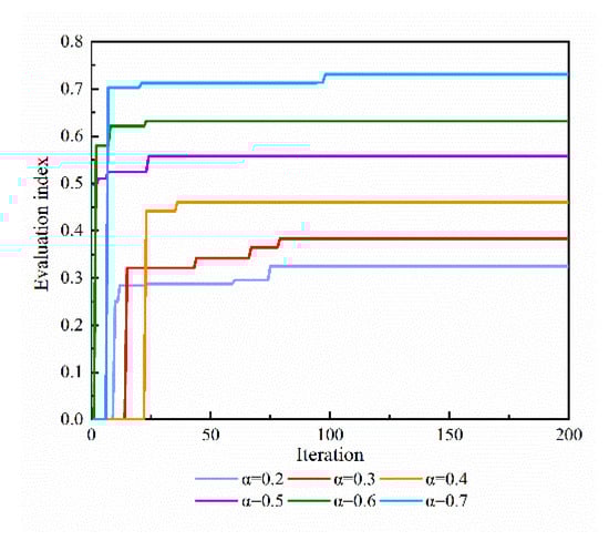
Figure 10. Convergence process of the algorithm under 6 situational advantage importance coefficients.

As shown in Figure 10, the convergence process of the algorithm differs significantly when different $\alpha$ values are used. This is because the importance of situational advantage reflects the psychological attitude of the pilot toward decision-making. The greater the value of $\alpha$ is, the more conservative the pilot. Therefore, the algorithm shows different convergence processes when different values of $\alpha$ are used.

Based on the threat matrix $\mathit{T}$ of the target against our aircraft and our situational advantage matrix $\mathit{S}$ against the enemy aircraft shown in Table 3 and Table 4, the target assignment results obtained under different values of $\alpha$ are shown in Table 5.

Table 5. Optimal target assignment scheme.

Target	1	2	3	4	5	6	7	8
$\alpha =0.2$	3	8	6	1	5	7	2	4
$\alpha =0.3$	5	8	4	2	7	1	6	3
$\alpha =0.4$	5	8	2	3	6	7	4	1
$\alpha =0.5$	7	3	5	4	1	2	6	8
$\alpha =0.6$	7	6	1	2	4	5	3	8
$\alpha =0.7$	6	2	5	1	7	3	4	8

(2) Mode 2: $m>n$

Assume that the eight aircraft in formation are coordinated to confront six enemy aircraft. All of our aircraft must be assigned a target, and each of them can be assigned only one target. Each target corresponds to at least one aircraft. Based on the situational information of both sides in operational confrontation at a certain moment, and with the help of the target threat assessment model, the threat matrix $\mathit{T}$ of the target against our aircraft and our situational advantage matrix $\mathit{S}$ against the enemy aircraft can be obtained, as shown in Table 6 and Table 7.

Table 6. Threat matrix of target aircraft against our aircraft.

Our Aircraft	Target
	1	2	3	4	5	6
1	0.3697	0.5879	0.1238	0.1789	0.2945	0.2395
2	0.1654	0.3196	0.3598	0.4256	0.4889	0.2451
3	0.4428	0.2006	0.2892	0.1549	0.1993	0.1993
4	0.2356	0.3249	0.3593	0.5269	0.2085	0.2654
5	0.1598	0.4740	0.2259	0.3892	0.1628	0.2847
6	0.1265	0.2358	0.2965	0.3492	0.2782	0.4892
7	0.3182	0.3459	0.2559	0.1274	0.3654	0.1952
8	0.1564	0.2682	0.4152	0.3027	0.2182	0.2027

Table 7. Situational advantage matrix of our aircraft against the target aircraft.

Our Aircraft	Target
	1	2	3	4	5	6
1	0.3265	0.4529	0.2458	0.1028	0.3316	0.2307
2	0.3689	0.5678	0.7521	0.4213	0.1895	0.2082
3	0.5361	0.2011	0.2356	0.1659	0.1879	0.3156
4	0.3187	0.2951	0.3275	0.1208	0.2685	0.2134
5	0.3490	0.2103	0.3516	0.6328	0.3598	0.2128
6	0.1553	0.2379	0.3341	0.1893	0.1466	0.2841
7	0.2172	0.4596	0.4520	0.2896	0.2029	0.2648
8	0.1905	0.3245	0.1124	0.4587	0.1526	0.2296

The importance of the target can be obtained from the threat matrix $\mathit{T}$ of the target against our aircraft and our situational advantage matrix $\mathit{S}$ against the enemy aircraft, as shown in Table 6 and Table 7.

$$({\alpha }_1,{\alpha }_2,{\alpha }_3,{\alpha }_4,{\alpha }_5,{\alpha }_6)=(0.1403,0.2139,0.2029,0.1841,0.1266,0.1322)$$

(43)

To analyze the influence of the situational advantage importance coefficient $\alpha$ on the convergence process of the algorithm, the convergence process of the algorithm is shown in Figure 11 when the values of $\alpha$ are 0.2, 0.3, 0.4, 0.5, 0.6, and 0.7.

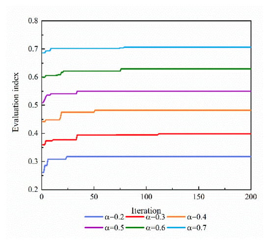
Figure 11. Convergence process of the algorithm with 6 importance coefficients of situational advantage.

A comparison of Figure 10 and Figure 11 indicates that under the conditions of different values of the importance coefficient of situational advantage, the starting values of the convergence curves of the algorithm are different. When the number of enemy aircraft and that of our aircraft are equal, the initial optimal fitness value of the algorithm is zero, which indicates that an assignment strategy that satisfies the constraints has not been found at the beginning of the algorithm, and when the number of aircraft is greater than that of the enemy aircraft, the initial optimal fitness of the algorithm is greater than zero, which indicates that the algorithm has already found a good assignment strategy that satisfies the constraints. The main reason for the above phenomenon is that when the position of the population individuals is initialized, the random generation method is used, and the random assignment is likely to cause repetitions. Thus, individuals that meet the constraint requirements are more likely to be generated when the number of enemy aircraft is unequal to that of the aircraft.

Based on the threat matrix $\mathit{T}$ of the target against our aircraft and our situational advantage matrix $\mathit{S}$ against the enemy aircraft shown in Table 6 and Table 7, the target assignment results obtained under different values of $\alpha$ are shown in Table 8.

Table 8. Optimal target assignment scheme.

Target	1	2	3	4	5	6
$\alpha =0.2$	5	3, 6	1	7, 8	4	2
$\alpha =0.3$	6	2	1, 5	7, 8	4	3
$\alpha =0.4$	5	6	1, 2	7	4, 8	3
$\alpha =0.5$	2	3, 8	1, 6	7	5	4
$\alpha =0.6$	8	7	2, 6	3	4, 5	1
$\alpha =0.7$	5	6	2, 4	8	1	3, 7

(3) Mode 3: $m<n$

Assume that the six aircraft in formation are coordinated to confront eight enemy aircraft. All of our aircraft must be assigned a target, and each of them can be assigned only one target. Each target corresponds to at least one aircraft. Based on the situational information of both sides in operational confrontation at a certain moment, and with the help of the target threat assessment model, the threat matrix $\mathit{T}$ of the target against our aircraft and our situational advantage matrix $\mathit{S}$ against the enemy aircraft can be obtained, as shown in Table 9 and Table 10.

Table 9. Threat matrix of target aircraft against our aircraft.

Our Aircraft	Target
	1	2	3	4	5	6	7	8
1	0.3567	0.4280	0.4285	0.4387	0.3323	0.4515	0.3463	0.3676
2	0.3943	0.3738	0.5111	0.5254	0.3626	0.4195	0.3221	0.3509
3	0.3692	0.4090	0.4901	0.4728	0.3605	0.6279	0.3655	0.4315
4	0.3564	0.4157	0.4161	0.3731	0.3427	0.3974	0.3047	0.2581
5	0.3544	0.5682	0.5828	0.4720	0.4630	0.6361	0.3933	0.4358
6	0.4982	0.4445	0.5046	0.4975	0.4464	0.5436	0.5058	0.4582

Table 10. Situational advantage matrix of our aircraft against the target aircraft.

Our Aircraft	Target
	1	2	3	4	5	6	7	8
1	0.4043	0.5994	0.4803	0.5529	0.4980	0.5138	0.5523	0.3949
2	0.4376	0.6214	0.6012	0.5641	0.4714	0.4162	0.5030	0.4129
3	0.5004	0.6360	0.6757	0.6506	0.6294	0.5576	0.5066	0.5554
4	0.5085	0.6752	0.6018	0.5470	0.6141	0.6230	0.6315	0.4629
5	0.2994	0.5596	0.4145	0.4293	0.2979	0.4396	0.4030	0.2801
6	0.5156	0.5868	0.5393	0.5572	0.5544	0.4147	0.5303	0.4532

The importance of the target can be obtained from the threat matrix $\mathit{T}$ of the target against our aircraft and our situational advantage matrix $\mathit{S}$ against the enemy aircraft, as shown in Table 9 and Table 10.

$$({\alpha }_1,{\alpha }_2,{\alpha }_3,{\alpha }_4,{\alpha }_5,{\alpha }_6,{\alpha }_7,{\alpha }_8)=(0.1130,0.1281,0.1424,0.1349,0.1120,0.1458,0.1493,0.1086)$$

(44)

In order to analyze the influence of the situational advantage importance coefficient $\alpha$ on the convergence process of the algorithm, the convergence process of the algorithm is shown in Figure 12 when the values of $\alpha$ are 0.2, 0.3, 0.4, 0.5, 0.6, and 0.7.

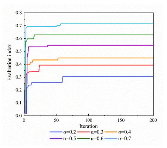
Figure 12. Convergence process of the algorithm with 6 situational advantage importance coefficients.

As shown in Figure 10, Figure 11 and Figure 12, the results of the target assignment vary under different values of the situational advantage importance coefficients. The results of the target assignment varied significantly under different modes.

Based on the threat matrix $\mathit{T}$ of the target against our aircraft and our situational advantage matrix $\mathit{S}$ against the enemy aircraft shown in Table 8 and Table 9, the target assignment results obtained under different values of $\alpha$ are shown in Table 11.

Table 11. Optimal target assignment scheme.

Target	1	2	3	4	5	6	7	8
$\alpha =0.2$	3	1	2	6	5	1	2	4
$\alpha =0.3$	3	1	4	5	5	2	1	6
$\alpha =0.4$	5	1	4	3	5	2	6	2
$\alpha =0.5$	4	3	5	1	5	2	3	6
$\alpha =0.6$	3	2	6	1	4	5	4	6
$\alpha =0.7$	6	3	2	2	5	1	4	5

From Table 5, Table 8 and Table 11, it can be observed that the modified salp swarm algorithm can effectively solve the target assignment problem in different modes and appropriate target assignment results can be obtained, indicating that the modified salp swarm algorithm is suitable for the multi-aircraft coordinated target assignment problem.

6.1.2. Dynamic Target Assignment in Different Modes

In the operational confrontation training process, both sides deployed a four-aircraft operational system. The confrontation trajectories of the enemy and the humans are shown in Figure 13.

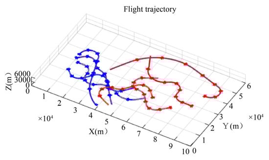
Figure 13. Diagram of the flight confrontation trajectory in the dynamic algorithmic example.

Figure 13 shows the 4V4 operational confrontation training trajectory. The duration of operation was 160 s. The enemy aircraft and our aircraft execute a target assignment and make decisions based on the preset tactical method. The red curve in Figure 11 represents our aircraft formation, and the blue curve represents the enemy aircraft formation.

To verify the effectiveness of the modified salp swarm algorithm in a dynamic environment, the CMASSA algorithm was used to assign targets dynamically with a computation interval of 5 s. The dynamic target assignment strategy is illustrated in Figure 14.

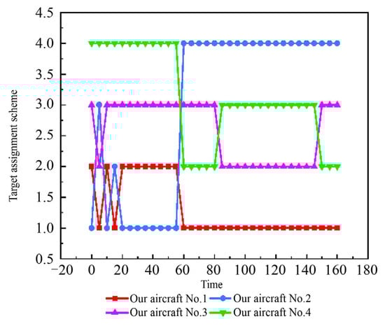
Figure 14. Dynamic target assignment.

Figure 14 indicates that, in the process of operational confrontation, our aircraft’s target assignment strategy changes as the situation of both sides constantly changes. Figure 15 provides a visualization of assignment outcomes.

Figure 15. Visualization of assignment outcomes.

The top-left graph shows the X-axis as the number of iterations, representing the CMASSA from generation 1 to generation 200, and the Y-axis is the assignment dimension, corresponding to the four target assignment variables (1–4) to be optimized. The mottled colors in early iterations indicate the algorithm’s exploration phase in which it attempts various assignment schemes. The color consistency in later iterations signifies that the algorithm has converged upon and stabilized at the optimal solution.

The upper-middle figure reflects how the threat values of the four target assignment variables change with iteration rounds. The initial fluctuations in the curve reflect the algorithm’s search process within the solution space. The changes in the curve’s slope at different iteration stages reflect the intensity of the algorithm’s adjustments to the assignment scheme. The curve’s tendency toward a horizontal straight line in the later stages indicates that the algorithm has reached a converged state.

The upper-right figure displays the fitness value curve over iterations, representing the quality of the target assignment schemes. The monotonically increasing or stable optimal fitness curve (black line) indicates the algorithm’s optimization effectiveness; the gap between the average fitness (blue dashed line) and optimal fitness reflects the overall population quality. The variation in the worst fitness (red dashed line) reflects the algorithm’s ability to maintain population diversity. As the algorithm progressively finds the optimal solution, its curve trend gradually stabilizes.

The bottom figure visualizes the four-dimensional optimization problem (four assignment dimensions) by projecting it into three-dimensional space. The transition of scatter points from dispersion to concentration reflects the algorithm’s shift from exploration to convergence. Additionally, the smoother trajectory in the later stages indicates the stability of the optimization process.

The operation situational advantage before and after the target assignment was compared and calculated to verify the rationality and effectiveness of the algorithm in dynamic target assignment. The comparison results are shown in Figure 16, in which the value of the situational advantage importance coefficient, $\alpha$, is 0.7.

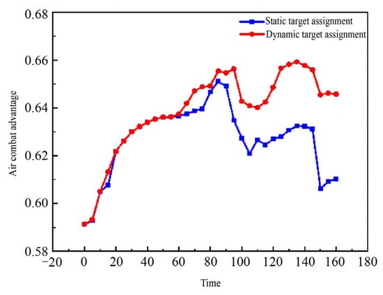
Figure 16. Comparison of situational advantage in dynamic target assignment.

From Figure 16, it can be observed that in the process of operational confrontation, the dynamic target assignment strategy obtained using the modified salp swarm algorithm can effectively enhance the situational advantage of our aircraft formation, which demonstrates that the CMASSA algorithm can effectively solve the dynamic target assignment problem. In terms of the real-time performance of the algorithm, the time required for the simulation based on the modified salp swarm algorithm in a dynamic environment is shown in Figure 17. The longest time was 0.7956 s, which satisfied the time requirement of actual operation, indicating that the algorithm has practical application value in actual operation.

Figure 17. Dynamic target assignment time of modified salp swarm algorithm.

6.2. Verifying the Effectiveness of Threat Evaluation When Sensor Measurement Errors Are Present

To simulate measurement errors in actual sensor systems, the experiment designed four types of noise models: position measurement noise, velocity measurement noise, angle measurement noise, and operational capability parameter noise. Position noise was set as a three-dimensional Gaussian distribution with standard deviations of 50, 50, and 10 meters; velocity noise had a standard deviation of 5 m/s; angle noise had a standard deviation of 2 degrees; and the standard deviation for operational capability parameter noise was 0.1. All noise was assumed to be zero-mean Gaussian white noise, with each noise source independent of the others. To ensure the reproducibility of the experimental results, a fixed random number seed was employed.

The core component of the experiment involves comparing the threat indices calculated from noise-free raw data and data with added noise. The threat assessment model comprehensively considers multiple dimensions, including the distance threat, angular threat, velocity threat, altitude threat, and operational capability threat, ultimately yielding a weighted composite threat index through integrated analysis. The same threat assessment algorithm was applied to both the raw data and the noisy data, producing two sets of corresponding threat assessment results, as shown in Figure 18.

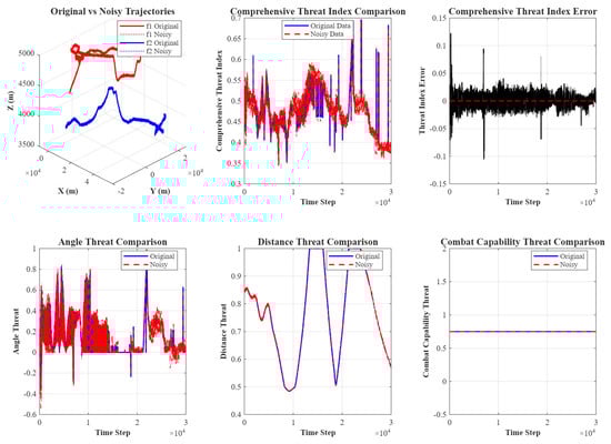
Figure 18. Two sets of corresponding threat assessment results.

The upper-left figure compares the noise trajectory with the original trajectory, simulating the sensor noise present in the actual processes. The middle-top figure shows the comparison of the integrated threat index. The curve indicates that under the experimental noise conditions described in the paper, the trend of the integrated threat index remains largely consistent with that of the noise-free scenario without any significant abrupt changes. The top-right figure displays the threat index error curve, revealing that errors are uniformly distributed on both sides of the zero value. This confirms that sensor noise under experimental conditions does not introduce systematic bias into the threat assessment. The bottom subplots, from left to right, display the variation curves of the angle, distance, and operational capability threat index components under noise. The impact of noise is significantly concentrated in the calculation of the angle threat index, while the distance and operational capability threat indices show negligible changes. However, no systematic bias is observed in the angle threat index either. Collectively, these results demonstrate that the threat assessment method described in this paper performs well under certain levels of sensor noise influence.

6.3. Verifying the Effectiveness of the Algorithm

6.3.1. Sensitivity Analysis of Chaos Mapping Initialization

The experiment selected nine chaotic initial values (C₁ = 0.1, 0.2, …, 0.9) covering the typical operating range of the logistic map. For each initial value, five independent replicate experiments were conducted under identical target assignment scenarios to eliminate random factors. The algorithm’s fundamental parameters were set as follows: 200 evolutionary generations, a population size of 10, and 4 optimization dimensions with values ranging from 1 to 4. To comprehensively evaluate the algorithm’s performance, analysis was conducted across four dimensions: the mean and standard deviation of the optimal fitness; convergence speed (the number of iterations required to reach 90% of the optimal fitness); average computation time; and the variability of the assignment results across each dimension, as illustrated in Figure 19.

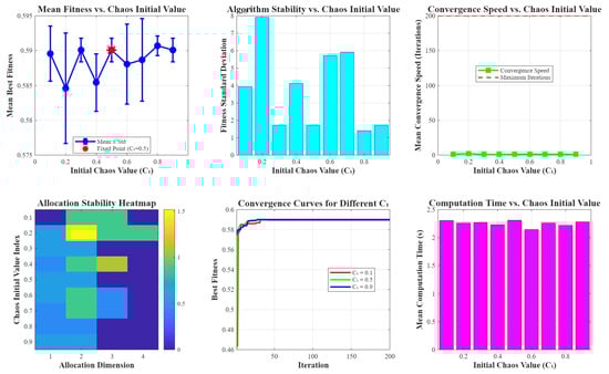
Figure 19. Initialization of sensitivity analysis results.

The upper-left figure shows the relationship between the average fitness and the chaotic initial values, while the upper-middle figure depicts the relationship between the fitness standard deviation and the chaotic initial values. It can be observed that as chaotic initial values change, fitness values exhibit a declining trend accompanied by an increase in the standard deviation. However, the logistic map exhibits stable chaotic properties with a fixed point at C₁ = 0.5. The upper-right figure illustrates the relationship between the convergence speed and the chaotic initial values. It is evident that the average convergence speed of the algorithm remains largely unchanged across different chaotic initial values and a maximum iteration count of 200. The lower-left figure displays a heatmap of assignment result stability. As the chaotic initial value increases, variability across different dimensions grows (darker colors indicate stronger variability), meaning assignment result stability decreases. However, stability remains relatively high at C₁ = 0.5. The middle panel displays convergence curves for the algorithm under different chaotic initial values. It can be observed that as C₁ increases, the algorithm’s performance slightly decreases. The right panel shows the algorithm’s runtime under different chaotic initial values. It can be seen that different chaotic initial values have little to no effect on the algorithm’s runtime.

6.3.2. Algorithm Effectiveness Under Complex Conditions

Two sets of experimental parameters with different complexities are listed in Table 12. In this table, $P_r$ represents the size of the salp population and $Gen$ represents the number of evolutionary generations of the algorithm. The $Num$ simulation experiments were conducted using the same simulation parameters to determine whether the performance of the algorithm was stable.

Table 12. Evolutionary parameter settings of the algorithm in two sets of experiments.

Mode	Experiment 1					Experiment 2
	$\mathit{m}$	$\mathit{n}$	${\mathit{P}}_{\mathit{r}}$	$\mathit{G}\mathit{e}\mathit{n}$	$\mathit{N}\mathit{u}\mathit{m}$	$\mathit{m}$	$\mathit{n}$	${\mathit{P}}_{\mathit{r}}$	$\mathit{G}\mathit{e}\mathit{n}$	$\mathit{N}\mathit{u}\mathit{m}$
$m=n$	16	16	50	200	20	24	24	50	200	10
$m>n$	20	16	50	200	20	30	24	50	200	10
$m<n$	16	20	50	200	20	24	30	50	200	10

To verify that the algorithm can effectively solve the target assignment problem in complex environments, five assessment indicators are defined to evaluate the performance of the algorithm.

(1) Average time: average running time of the algorithm $T_{aver}$:

$$T_{aver}={\displaystyle \sum _{i=1}^n{T}_i}/Num$$

(45)

(2) Average gain: the average optimal fitness over multiple simulation experiments $I_{aver}$:

$$I_{aver}={\displaystyle \sum _{i=1}^n{I}_i}/Num$$

(46)

(3) Optimal gain: the maximum fitness value over multiple simulation experiments $I_{best}$:

$$I_{best}=\underset{i=1}{\overset{Num}{\max }}{I}_i$$

(47)

(4) Constraint violation: During the iterations of the algorithm, the number of constraint violations $addnum$ of the obtained optimal solution is divided by the maximum number of iterations $T_{\max }$ to obtain the percentage $P_b$:

$$P_b=addnum/T_{\max }$$

(48)

(5) Optimal solution variance: the variance in the optimal solution $best$ obtained from multiple simulations of the algorithm ${\sigma }_{best}$:

$${\sigma }_{best}=var(best)$$

(49)

Table 13 records the two sets of experimental data corresponding to the value $\alpha =0.7$ of the situational advantage importance coefficient. The following conclusions of the simulation experiments are obtained:

Table 13. Statistical data on the assignment results of the two sets of experiments.

Experiment	Mode	Average Time	Average Gain	Optimal Gain	Constraint Violation	Optimal Solution Variance
Experiment 1	$m=n$	4.5248	0.7295	0.7468	4.59%	6.6327 × 10−5
	$m>n$	5.8367	0.7137	0.7268	4.17%	3.2325 × 10−5
	$m<n$	8.2039	0.7251	0.7365	2.14%	4.1578 × 10−5
Experiment 2	$m=n$	7.3081	0.9263	0.9453	6.23%	8.2435 × 10−5
	$m>n$	10.2196	0.8734	0.9042	7.16%	4.1365 × 10−4
	$m<n$	13.8026	0.8109	0.8364	5.26%	1.2684 × 10−4

(1) Experiments 1 and 2 obtained satisfactorily better target assignment results, indicating that the modified salp swarm algorithm can effectively solve the multi-aircraft coordinated target assignment problem in different modes.

(2) Both Experiment 1 and Experiment 2 increased the number of enemy aircraft and our aircraft based on Section 6.1. Although the running time of the CMASSA algorithm is increased, it can find the optimal solution in an effective time, indicating that the modified salp swarm algorithm can effectively solve the multi-aircraft coordinated target assignment problem under complex conditions.

(3) In the two sets of simulation experiments, the gap between the average and optimal gains of each mode was extremely small, indicating that the search results of the algorithm were close to the globally optimal solution.

(4) The low constraint violation rate of the algorithm indicates that the modified salp swarm algorithm is suitable for the multi-aircraft coordinated target assignment problem. The low variance in the optimal solution indicates that the algorithm exhibits good stability.

6.4. CMASSA Algorithm Performance

This section analyses the performance of the CMASSA algorithm in solving the multi-aircraft coordinated target assignment problem from two aspects: the convergence curve of the simulation experiment and the average fitness of the population during the algorithm iteration process. In this study, the performances of the CMASSA algorithm, modified genetic algorithm (GA) [25], modified particle swarm optimization (PSO) [26], and modified ant colony optimization (ACO) [27] were evaluated to solve the multi-aircraft coordinated target assignment problem. The performance parameters are shown in Table 14. The convergence curve in a single simulation and the average convergence curve in multiple simulations for the target assignment based on the four algorithms are shown in Figure 20 and Figure 21, respectively.

Table 14. Comparison between the CMASSA algorithm and other algorithms.

Mode	Methods	Number of Aircraft	Population Number	Iteration Times	Experiment Times	Average Time	Average Gain	Optimum Gain	Optimal Solution Variance
$m=n$	GA	$\begin{array}{l}m=8\\ n=8\end{array}$	50	200	20	5.6027	0.5088	0.7347	0.1079
	CMASSA		50	200	20	2.5824	0.7125	0.7309	0.0078
	PSO		50	200	20	5.7294	0.5258	0.7038	0.0903
	ACO		50	200	20	1.8527	0.7285	0.7406	3.3664 × 10−5
$m>n$	GA	$\begin{array}{l}m=8\\ n=6\end{array}$	50	200	20	9.6301	0.7157	0.7267	2.5787 × 10−5
	CMASSA		50	200	20	8.0516	0.7209	0.7224	1.6451 × 10−5
	PSO		50	200	20	7.7590	0.7169	0.7228	4.3039 × 10−5
	ACO		50	200	20	5.2712	0.7229	0.7311	1.1720 × 10−5
$m<n$	GA	$\begin{array}{l}m=6\\ n=8\end{array}$	50	200	20	10.4380	0.7167	0.7247	7.9346 × 10−5
	CMASSA		50	200	20	8.2359	0.7208	0.7231	1.9133 × 10−5
	PSO		50	200	20	11.7663	0.7177	0.7183	3.5426 × 10−5
	ACO		50	200	20	5.1259	0.7244	0.7304	1.5330 × 10−5

Figure 20. Single convergence curve of the target assignment results.

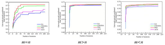
Figure 21. Average convergence curve of different algorithms.

The modified salp swarm algorithm is compared with the modified GA, PSO, and ACO algorithms. The population size, number of iterations, and number of repetitions for all four algorithms were the same when the simulation experiments were performed. Table 14 and Figure 20 and Figure 21 indicate that the CMASSA algorithm obtains the largest gain in the multi-aircraft target assignment strategy, indicating that the target assignment scheme obtained using this algorithm is more reasonable. According to the convergence curve of the algorithm, the CMASSA algorithm had the fastest convergence rate and shortest average running time. The other three algorithms can also obtain a target assignment strategy with a large gain; however, the execution time of these algorithms is too long, and the stability of the optimal schemes obtained by these algorithms is insufficient compared with the CMASSA algorithm. Although the modified GA, PSO, and ACO algorithms address the dilemma of getting stuck in local optima through parameter tuning or strategy introduction, their core mechanisms may still prove inadequate when tackling the multi-constraint target assignment problem described in this paper. The CMASSA algorithm significantly enhances the ability of individuals to escape local optimum regions by incorporating strategies such as combinatorial mutation mechanisms and adaptive inertial weights, thereby increasing the probability of discovering global optima or higher-quality solutions.

7. Conclusions

This paper proposes an improved chaotic mutation adaptive salp swarm algorithm to address the target assignment problem in multi-aircraft scenarios coordinated in complex environments. The research aims to enhance the algorithm’s performance in solving such multi-constraint optimization problems. The main research work is summarized as follows:

7.1. Key Research Findings and Innovations

The primary contributions lie in two dimensions: model construction and algorithmic improvement. Model-wise, this work overcomes the limitations of traditional single-aircraft advantage assessments by establishing a multi-aircraft coordinated advantage assessment model that incorporates formation synergy factors, yielding target assignment outcomes more aligned with real-world operational logic. Algorithmically, three key enhancements were made to the salp swarm algorithm: a chaotic search strategy with a contraction mechanism was introduced to strengthen global exploration capabilities, a Gaussian–Cauchy combined mutation strategy was adopted to improve local exploitation and population diversity, and an adaptive inertia weight mechanism was designed to dynamically balance exploration and exploitation processes. Additionally, a penalty function method seamlessly integrated constraints into the fitness function, simplifying problem complexity. Simulation experiments demonstrate that CMASSA achieves high collaborative operational effectiveness across three typical engagement patterns (m = n, m > n, m < n), exhibiting superior convergence speed and stability to the modified genetic algorithm, particle swarm optimization, and ant colony optimization used for comparison.

7.2. Research Limitations and Future Prospects

Despite the achievements outlined above, this study retains certain limitations. First, the current model assumes static operational conditions, neglecting dynamic factors such as aircraft maneuvering, missile flight times, and sequential decision-making timelines. Second, while algorithm validation considered formation-coordinated effectiveness, it did not sufficiently account for the impact of formation tactics. Furthermore, comparative analysis with cutting-edge AI methods (e.g., deep reinforcement learning) remains insufficient.

In summary, the CMASSA algorithm proposed in this study provides an effective solution for multi-aircraft cooperative target assignment problems. Theoretical analysis and simulation experiments validate its advantages in enhancing cooperative effectiveness and convergence performance. Although the model requires refinement in certain aspects, it lays a solid foundation for subsequent research in this field, demonstrating clear theoretical significance and application prospects.

References

- Li, W.; Fang, F.; Wang, Z.; Zhu, Y.; Peng, D. Intelligent maneuvering decision-making in two-UCAV cooperative air combat based on improved MADDPG with hybrid hyper network. Acta Aeronaut. Astronaut. Sin. 2024, 45, 529460. [Google Scholar]
- Ma, S.; Zhang, H.; Yang, G. Target threat level assessment based on cloud model under fuzzy and uncertain conditions in air combat simulation. Aerosp. Sci. Technol. 2017, 67, 49–53. [Google Scholar] [CrossRef]
- Moon, S.; Oh, E.; Shim, D.H. An integral framework of task assignment and path planning for multiple unmanned aerial vehicles in dynamic environments. J. Intell. Robot. Syst. 2013, 70, 303–313. [Google Scholar] [CrossRef]
- Zhang, J.; Guo, H.; Chen, T. Improvement in Hungarian Algorithm for Assignment Problem. Acta Armamentarii 2021, 42, 1339–1344. [Google Scholar]
- Luitpold, B. Coordinated Target Assignment and UAV Path Planning with Timing Constraints. J. Intell. Robot. Syst. 2019, 3, 857–869. [Google Scholar]
- Yi, X.; Zhu, A. An improved neuro-dynamics-based approach to online path planning for multi-robots in unknown dynamic environments. In Proceedings of the IEEE International Conference on Robotics and Biomimetics, Shenzhen, China, 12–14 December 2013; pp. 1–6. [Google Scholar]
- ElGibreen, H.; Youcef-Toumi, K. Dynamic task allocation in an uncertain environment with heterogeneous multi-agents. Auton. Robot. 2019, 43, 1639–1664. [Google Scholar] [CrossRef]
- Hunt, S.; Meng, Q.; Hinde, C. A Consensus-Based Grouping Algorithm for Multi-agent Cooperative Task Allocation with Complex Requirements. Cogn. Comput. 2014, 6, 338–350. [Google Scholar] [CrossRef]
- Qing, L.; Liu, Y.; Zeng, D. Target allocation method based on multi-objective particle swarm optimization algorithm. In Proceedings of the International Conference on Algorithm, Imaging Processing, and Machine Vision (AIPMV 2023), Qingdao, China, 9 January 2023; pp. 72–81. [Google Scholar]
- Li, J.; Yang, X.; Yang, Y.; Liu, X. Cooperative mapping task assignment of heterogeneous multi-UAV using an improved genetic algorithm. Knowl.-Based Syst. 2024, 296, 111830. [Google Scholar] [CrossRef]
- Alencar, R.C.; Santana, C.J.; Bastos-Filho, C.J. Optimizing Routes for Medicine Distribution Using Team Ant Colony System. Adv. Intell. Syst. Comput. 2020, 923, 40–49. [Google Scholar]
- Whitbrook, A.; Meng, Q.; Chung, P.W. Addressing robustness in time-critical, distributed, task allocation algorithms. Appl. Intell. 2019, 49, 1–15. [Google Scholar] [CrossRef]
- Xue, Y.; Jiang, B.; Huang, Y. Optimization strategy for multi-AGV multi-task assignment scheduling based on improved particle swarm genetic algorithm. In Proceedings of the 5th International Conference on Artificial Intelligence and Advanced Manufacturing, Brussels, Belgium, 20–21 October 2023; pp. 131–138. [Google Scholar]
- Chen, C.; Quan, W.; Shao, Z. Aerial Target Threat Assessment Based on Gated Recurrent Unit and Self-Attention Mechanism. J. Syst. Eng. Electron. 2024, 35, 361–373. [Google Scholar] [CrossRef]
- Sheng, L.; Li, L.; Wu, H.; Wang, P. Target Threat Assessment in Air Combat with BP Neural Network for UAV. J. Phys. Conf. Ser. 2023, 2506, 012010. [Google Scholar] [CrossRef]
- Kojadinovic, I.; Marichal, J.L. Entropy of bi-capacities. Eur. J. Oper. Res. 2007, 178, 164–184. [Google Scholar] [CrossRef]
- Ugajin, T. Mutual information of excited states and relative entropy of two disjoint subsystems in CFT. J. High Energy Phys. 2017, 2017, 184. [Google Scholar] [CrossRef]
- Panwar, K.; Deep, K. Discrete Salp Swarm Algorithm for Euclidean Travelling Salesman Problem. Appl. Intell. 2023, 53, 11420–11438. [Google Scholar] [CrossRef]
- Prajisha, C.; Vasudevan, A.R. An efficient intrusion detection system for MQTT-IoT using enhanced chaotic salp swarm algorithm and LightGBM. Int. J. Inf. Secur. 2022, 21, 1263–1282. [Google Scholar] [CrossRef]
- Xu, H.; Zhang, A.; Bi, W.; Xu, S. Dynamic Gaussian mutation beetle swarm optimization method for large-scale weapon target assignment problems. Appl. Soft Comput. 2024, 162, 111798. [Google Scholar] [CrossRef]
- Hadikhani, P.; Lai, D.T.C.; Ong, W.H. A Novel Skeleton-Based Human Activity Discovery Using Particle Swarm Optimization with Gaussian Mutation. IEEE Trans. Hum.-Mach. Syst. 2023, 53, 538–548. [Google Scholar] [CrossRef]
- Wu, L.; Wu, J.; Wang, T. The improved grasshopper optimization algorithm with Cauchy mutation strategy and random weight operator for solving optimization problems. Evol. Intell. 2024, 17, 1751–1781. [Google Scholar] [CrossRef]
- Nithyanandam, C.; Mohankumar, G. Research on aircraft landing schedule using opposition-based genetic algorithm with Cauchy mutation. Int. J. Bus. Intell. Data Min. 2020, 16, 89–106. [Google Scholar] [CrossRef]
- Zong, Q.; QIN, X.; ZHANG, B.; Tian, B.; Dandan, W. Cooperative Task Allocation of Large-Scale UCAV Based on DPSO-GT-SA Algorithm. J. Tianjin Univ. (Sci. Technol.) 2018, 10, 7–11. [Google Scholar]
- Zhao, Y.; Chen, Y.; Zhen, Z.; Jiang, J. Multi-weapon multi-target assignment based on hybrid genetic algorithm in uncertain environment. Int. J. Adv. Robot. Syst. 2020, 17, 1–16. [Google Scholar] [CrossRef]
- Zhou, X.; Yang, K. Cooperative multi-task assignment modeling of UAV based on particle swarm optimization. Intell. Decis. Technol. 2024, 18, 919–934. [Google Scholar] [CrossRef]
- Li, Y.; Zhang, S.; Chen, J.; Jiang, T.; Ye, F. Multi-UAV Cooperative Mission Assignment Algorithm Based on ACO method. In Proceedings of the 2020 International Conference on Computing, Networking and Communications (ICNC), Big Island, HI, USA, 17–20 February 2020; pp. 304–308. [Google Scholar]
Disclaimer/Publisher’s Note: The statements, opinions and data contained in all publications are solely those of the individual author(s) and contributor(s) and not of MDPI and/or the editor(s). MDPI and/or the editor(s) disclaim responsibility for any injury to people or property resulting from any ideas, methods, instructions or products referred to in the content. |
© 2025 by the authors. Licensee MDPI, Basel, Switzerland. This article is an open access article distributed under the terms and conditions of the Creative Commons Attribution (CC BY) license.