A Hybrid Algorithm Modeling on Test-Bench Data for Light-Duty Afterburning Turbojet Engine

Abstract

For highly maneuverable aircraft, the afterburning engine serves as a core and critical component. Due to the complex structure of the afterburner and the strong coupling among parameters, mechanism-based modeling of afterburning engines remains extremely challenging. To address this problem, this paper proposes a data-driven hybrid algorithm modeling framework for a light-duty afterburning turbojet engine. Using test-bench data from the TWP220L light-duty afterburning turbojet, two hybrid algorithm models were developed: (i) PSO-DNN and (ii) NGO-LSSVM. Four models, DNN, PSO-DNN, LSSVM, and NGO-LSSVM, were compared by mapping engine input parameters (altitude, Mach number, rotor speed, and fuel flow rate) to two key performance outputs (thrust and turbine pressure ratio). Based on visual error analysis and regression evaluation metrics, it was found that the optimized algorithm significantly reduced the prediction error. The NGO-LSSVM model achieved the highest accuracy in both performance indicators, increasing R² by 5.3% for thrust, and increasing R² by 6.8% for turbine pressure ratio. This framework offers a practical and high-precision approach for light-duty afterburning engine performance prediction and lays a foundation for the development of model-based and data-driven onboard control strategies.

1. Introduction

With the continuous evolution of modern aeronautical technology, the requirements for aircraft performance have escalated significantly. As the core power component of an aircraft, the engine exerts a decisive influence on the overall performance of the airframe. As shown in Figure 1, an afterburning engine is a propulsion device developed on the basis of a turbojet or turbofan, featuring an additional afterburner installed downstream of the turbine. Although the afterburner accounts for only about 20% of the engine’s total mass, it can provide an additional 30–50% thrust augmentation in a short period of time [1], enabling the aircraft to attain enhanced power and maneuverability under high-load conditions such as takeoff, climb, supersonic cruise, and combat maneuvers.

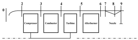
Figure 1. Schematic diagram of the structure of an afterburning turbojet engine.

Afterburning engines have become an indispensable component of modern defense equipment. The afterburner is directly related to an aircraft’s tactical maneuverability and combat radius. In air-superiority fighters, supersonic interceptors, and target drones [2,3], the instantaneous thrust augmentation provided by the afterburner is employed for supersonic sprints, short-field takeoffs and landings, rapid climbs, and high-G maneuvers. These capabilities are critical for determining air-combat effectiveness, mission execution efficiency, and overall battlefield survivability. Consequently, afterburning engines occupy an extremely important position in aerospace propulsion, especially in military high-speed fighters. Accordingly, accurately characterizing both the transient and steady-state behaviors of afterburning and representing them as identifiable dynamic models is essential for achieving reliable control, performance optimization, and real-time engine management.

In recent years, aero-engine modeling and control have advanced rapidly, with substantial progress in component-based simulation, data-driven prediction, hybrid modeling frameworks, and intelligent algorithms for dynamic performance estimation.

In the area of component-based modeling and control, Wang et al. [4] constructed a numerical simulation model for a single-spool turbojet engine based on the component method, performing systematic calculations at both design and off-design points. The results exhibited high consistency with experimental data, verifying the reliability of the model. Pan et al. [5] established a turbofan engine model considering volume effects and proposed a heat transfer mechanism model for the turbine component. The results showed that compared with traditional models, this approach significantly improved the dynamic simulation capability of engine parameters. Shi et al. [6] developed a full-envelope steady-state mathematical model for an afterburning twin-spool mixed-flow turbofan engine based on the component method. This modeling approach accurately performs steady-state calculations and full-state dynamic simulations across the entire flight envelope, effectively reflecting the engine’s working process throughout all operating conditions. Xia et al. [7] conducted dynamic simulations in Simulink, verifying the correctness of the model through experimental data curves, thus establishing a flexible simulation platform for engine control system and fault diagnosis research.

Recent research has increasingly focused on hybrid modeling approaches that combine mechanism-based and data-driven methods to improve aero-engine modeling accuracy. Li et al. [8] proposed a hybrid model combining mechanism-based and neural-network-based data-driven approaches for gas turbine modeling. The average relative error of all parameters was within 1.5%, and the relative error of the compressor outlet and power turbine outlet temperatures was less than 0.5%, demonstrating high accuracy. You et al. [9] proposed a 3-D attention-enhanced hybrid neural network combining CNN and BiLSTM for turbofan engine RUL prediction. The model integrates spatial–channel attention and handcrafted degradation features, achieving superior interpretability, robustness, and accuracy on the C-MAPSS dataset compared to existing methods. Zhao et al. [10] proposed a size-transferring RBF network for thrust estimation, enabling adaptive generalization across engine sizes and operating points through nonlinear mapping and PSO-based optimization.

Recent studies have also explored predictive modeling of aero-engines and their components. Alozie et al. [11] developed an adaptive model-based framework for gas turbine prognostics and remaining useful life (RUL) prediction, combining system behavior and degradation characteristics to improve fault prognostics in aircraft engines. Xue et al. [12] proposed a deep learning-based predictive maintenance strategy using LSTM and Transformer architectures to enhance engine health prediction performance. A prediction-focused machine learning method was introduced to adapt aero gas turbine performance models under steady and transient conditions. Deep convolutional neural network approaches have been applied to turbofan engine remaining useful life estimation [13], and general machine learning surrogate models have been developed for gas turbine performance prediction across operational regimes [14].

Advanced deep learning and intelligent control algorithms have been explored to enhance engine modeling and control performance. Gao et al. [15] proposed an innovative control strategy based on deep reinforcement learning, employing the Deep Deterministic Policy Gradient (DDPG) algorithm to update neural network parameters, and introducing a complementary integrator to eliminate steady-state bias caused by neural approximation errors, thereby significantly improving engine acceleration performance. Zheng et al. [16] developed an onboard aero-engine model using a Batch-Normalized Deep Neural Network, enhancing convergence stability and prediction robustness for real-time engine performance estimation under varying flight conditions. Harris et al. [17] employed artificial neural networks to identify nonlinear performance relationships in aircraft engines, demonstrating superior accuracy and adaptability compared to conventional component-based models across diverse operating regimes.

Beyond direct control applications, a significant body of literature has leveraged engine modeling for Prognostics and Health Management (PHM). Du et al. [18] introduced an ensemble Least Squares Support Vector Machine (LSSVM) framework to predict chaotic aero-engine parameters, utilizing multiple kernel integrations to improve generalization and capture nonlinear system dynamics effectively. Huang et al. [19] designed a digital twin model integrating physical and deep multimodal data, achieving accurate fault diagnosis by fusing sensor, operational, and simulation information through deep representation learning. Loboda et al. [20] developed simplified data-driven models for gas turbine diagnostics, reducing computational complexity while maintaining diagnostic accuracy through efficient feature extraction and regression-based modeling. While these contributions are substantial for health monitoring, they primarily focus on long-term degradation trends or steady-state fault isolation. There remains a paucity of research specifically targeting the high-frequency dynamic modeling required for the precise control of light-duty afterburning turbojet engines, particularly during rapid transient phases.

Significant progress has been made by researchers both domestically and abroad in these areas. However, several problems remain:

• Most existing studies focus on single-method modeling or steady-state characteristic simulation of non-afterburning engines. Research on dynamic modeling and control of light-duty afterburning turbojet engines under afterburning conditions remains relatively limited.
• In data-driven engine modeling, many studies have employed algorithms such as neural networks and deep learning. With the continuous advancement of computational technology, traditional algorithms have gradually revealed limitations in efficiency and accuracy.

To address these gaps, this study develops a data-driven hybrid modeling framework that integrates an intelligent optimization algorithm with a nonlinear regression model to enhance the identification accuracy of afterburning engine dynamics. Section 2 analyzes the main challenges of afterburning engine modeling. Section 3 introduces the fundamental principles and optimization mechanisms of the hybrid algorithm. Section 4 presents the model construction process and result analysis.

The results demonstrate that the proposed hybrid model can effectively capture the transient and steady-state characteristics of a light-duty afterburning turbojet engine, achieving superior prediction accuracy and generalization capability compared with conventional approaches. This study contributes a novel hybrid modeling methodology tailored specifically for afterburning engines, providing a more accurate, data-efficient, and practically deployable solution for onboard modeling and control.

2. Problem Description and Solution Strategy

The complex internal flow field and strong parameter coupling of afterburning engines, traditional mechanism-based modeling methods are difficult to achieve high-precision characterization [21]. Although the component-based method can effectively reflect the physical structure of the engine, it requires extensive experimental calibration and simplifying assumptions when dealing with various complex coupling effects. This inevitably limits the accuracy and generalization capability of the model.

Figure 2 illustrates the structure and operating characteristics of the afterburner in a turbojet engine. As shown at the location marked by red circle 1, the airflow, after expanding through the turbine and performing work, enters the afterburner. At this point, the gas pressure is low and the flow velocity is high, making ignition difficult. The region marked by red circle 2 is near the fuel injection area [22]. The afterburner is very sensitive to changes in fuel flow, and the geometry of the flame stabilizer is limited by the volume of the afterburner. Therefore, flame stability is particularly critical and difficult to model.

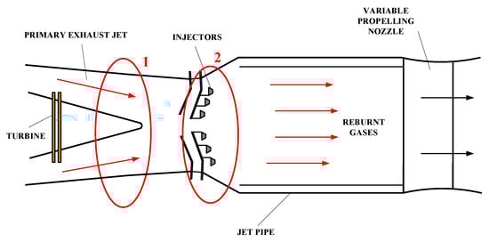
Figure 2. The structure of the afterburner of an afterburning turbojet engine.

With the increasing development of data-driven techniques in the field of aero-engine modeling, algorithms such as Deep Neural Networks (DNN) and Support Vector Machines (SVM) have achieved notable success in performance prediction. They have also exhibited limitations, including low computational efficiency, insufficient accuracy, and high sensitivity to hyperparameters, which often lead to local optima and unstable convergence during training.

To address above problems, this study proposes the following approaches:

• Considering the complexity of the afterburning engine mechanism and the strong coupling among its parameters, a data-driven modeling approach is adopted. By utilizing experimental test data to establish nonlinear mappings, the dynamic characteristics of the engine under afterburning conditions can be effectively captured without relying on precise physical models.
• To overcome the limitations of traditional algorithms in terms of efficiency and accuracy, a hybrid algorithmic framework is introduced, which integrates optimization algorithms with traditional algorithm models. Through the synergy of global parameter optimization and local learning, this approach enhances the fitting accuracy and training stability, providing a feasible solution for high-precision modeling of complex nonlinear systems.

Engine performance modeling not only enables rapid prediction of key indicators such as thrust, efficiency, and fuel consumption but also provides essential data support for aircraft overall design, flight trajectory simulation, and mission planning. This study explores a novel high-precision modeling framework for light-duty afterburning turbojet engines from the perspectives of data-driven modeling and algorithmic fusion, providing a new technical pathway for dynamic modeling and intelligent control of afterburning propulsion systems.

3. Theoretical Foundation

3.1. Traditional Modeling and Data-Driven Modeling

Control strategies for aeroengines are commonly categorized into two major types: model-based control and data-driven control. The former relies on accurate modeling of the controlled system’s dynamics, i.e., the construction of high-fidelity white-box mechanism models. When such models sufficiently reflect the real dynamic behavior of the engine, model-based approaches can achieve excellent control performance. In practical afterburning aeroengine architectures, the placement of onboard sensors is constrained, limiting the variety of measurable parameters and the number of measurement stations. In addition, the introduction of the afterburner imparts strong nonlinearity and tight multivariable coupling to the system, which poses significant challenges to the accuracy and practicality of traditional physics-based modeling methods.

For complex systems where precise mechanism models are difficult to obtain, data-driven control methods offer distinct advantages [23]. These approaches do not require a complete physical description of the system. Instead, they learn from experimental and operational data and employ statistical modeling or machine learning algorithms (e.g., neural networks, regression models) to directly establish input–output mappings for performance prediction and control law design. Using existing test data, data-driven modeling methods (such as neural networks) can fit the dynamic characteristics of afterburning engines, providing the accuracy required for engineering and providing a feasible basis for the development of subsequent control strategies.

Given the strong multivariable coupling and highly dynamic operating conditions of afterburning aeroengines, traditional mechanism-based modeling exhibits clear limitations in characterizing afterburner behavior. Therefore, this study adopts a data-driven modeling approach to fully exploit the statistical features of test and operational data, with the aim of achieving accurate modeling and prediction of afterburner dynamics under complex operating conditions.

3.2. Working Mechanism of Afterburning Engines

When the aircraft throttle lever is at the maximum position, the main part of the engine produces maximum thrust. If further thrust increase is desired, for an afterburning engine, the throttle can be pushed beyond the maximum position into the afterburner range to activate the afterburning mode. During the transition from the maximum state to the afterburning state, the parameters before the afterburner and the engine’s rotor speed remain at their maximum values, thereby increasing the thrust on the basis of maximum thrust. [24] For a variable-nozzle afterburning engine, when the afterburner is engaged, the nozzle exit area must be correspondingly enlarged to ensure that the turbine pressure ratio remains unchanged, so that the compressor and turbine of the main engine continue to operate unaffected. The following are the flow balance equations for the critical section of the turbine guide vanes and the critical section of the nozzle under afterburning and non-afterburning conditions [25].

During afterburning:

$$A_{nb}{\sigma }_{nb}{\displaystyle \frac{p_{t4}}{\sqrt{T_{t4}}}}q\left({\lambda }_{nb}\right)=A_{8 ab}{\sigma }_{ab}{\sigma }_e{\displaystyle \frac{p_{t5}}{\sqrt{T_{t,ab}}}}q\left({\lambda }_8\right)$$

(1)

During non-afterburning:

$$A_{nb}{\sigma }_{nb}{\displaystyle \frac{p_{t4}}{\sqrt{T_{t4}}}}q\left({\lambda }_{nb}\right)=A_8{\sigma }_{ab}{\sigma }_e{\displaystyle \frac{p_{t5}}{\sqrt{T_{t5}}}}q\left({\lambda }_8\right)$$

(2)

where $A_{nb}$, $A_{8 ab}$, and $A_8$ represent the critical cross-sectional areas of the turbine nozzle guide vanes, and the nozzle under afterburning and non-afterburning conditions, respectively, $q\left({\lambda }_{nb}\right)$ and $q\left({\lambda }_8\right)$ denote the aerodynamic flow functions at the critical sections of the turbine nozzle and the exhaust nozzle. Assuming both sections are in critical or overcritical conditions, $q\left({\lambda }_{nb}\right)=q\left({\lambda }_8\right)=1.0$. ${\sigma }_{nb}$, ${\sigma }_{ab}$, and ${\sigma }_e$ are the total pressure recovery coefficients of the turbine nozzle, afterburner, and exhaust nozzle, respectively, and are assumed to be constants.

By dividing the two equations, we obtain

$${\displaystyle \frac{A_{8 ab}}{A_8}}=\sqrt{{\displaystyle \frac{T_{t,ab}}{T_{t5}}}}$$

(3)

This equation indicates that after the afterburner is ignited, the total temperature at the inlet of the exhaust nozzle increases. $T_{t5}$ is the total inlet temperature of the exhaust nozzle without afterburning. $T_{t,ab}$ is the temperature after afterburner is engaged. If $A_8$ remains unchanged, the total pressure $p_{t5}$ behind the turbine will increase, leading to a reduction in the turbine pressure ratio ${\pi }_T$, which affects the coordinated operation of the main components and prevents the engine from reaching the rotor speed corresponding to the maximum thrust state.

Therefore, when the engine geometry is fixed ($A_{8,ab}=\mathrm{const}$), one possible control strategy is

$$\left.\begin{array}{c}{W}_f\to n=n_{max}=const\\ W_{f,ab}\to {\pi }_T=const\\ \left(A_{8,ab}=const\right)\end{array}\right\}$$

(4)

When flight conditions change, the engine control system adjusts the main combustor fuel flow $W_f$ to maintain the rotor speed $n=n_{max}$ constant, and regulates the afterburner fuel flow $W_{f,ab}$ to keep the turbine pressure ratio ${\pi }_T=\mathrm{const}$, while the engine geometry remains unchanged($A_{8,ab}=\mathrm{const}$).

Figure 3 presents the variation in fuel flow during a set of TWP220L light-duty afterburning turbojet tests. To facilitate detailed analysis, the fourth test cycle is magnified. Each afterburning process lasts approximately 30–40 s. During the ignition phase, the fuel flow rapidly rises to about 110 kg/h, exhibiting a distinct step increase. After approximately 10 s, the fuel flow increases by an additional 40 kg/h, indicating the transition to the partial afterburning stage, which serves as an intermediate phase between ignition and full afterburning. About 6 s later, the fuel flow rises again, and the engine enters the full afterburning mode. In this stage, the fuel flow gradually increases from 180 to approximately 190 kg/h and remains nearly steady for about 20 s. Finally, as the afterburner is shut down, the fuel flow gradually decreases, and the engine returns to a steady operating state. This sequence comprehensively characterizes the dynamic evolution of ignition, partial afterburning transition, full afterburning, and afterburner shutdown.

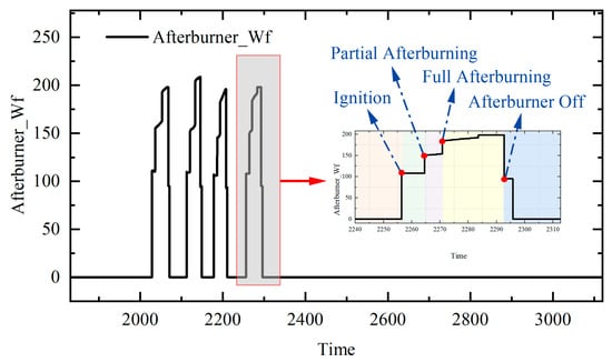
Figure 3. Afterburner fuel variation trend during the afterburning process.

3.3. Hybrid Algorithm

3.3.1. The Introduction of Hybrid Algorithms

Hybrid algorithms combine the strengths of multiple approaches to achieve complementary and enhanced performance. A single algorithm is often constrained by limitations in search capability, convergence speed, or generalization ability. By integrating global exploration and local exploitation, hybrid algorithms can achieve a better balance between accuracy and stability. Specifically, heuristic optimization methods are employed for global exploration of the solution space, while machine learning models are used to approximate the objective function with high precision. The integration of these techniques significantly improves convergence efficiency and robustness. Moreover, hybrid algorithms exhibit superior adaptability and generalization in solving complex nonlinear, multimodal, and high-dimensional problems, making them widely applicable in engineering optimization and intelligent modeling.

3.3.2. PSO-DNN

Particle Swarm Optimization (PSO) is a swarm intelligence-based optimization algorithm, originally proposed by James Kennedy and Russell Eberhart [26] in 1995. This algorithm was initially inspired by the regularity of bird flocking behavior, and then used a simplified model built using swarm intelligence. Based on the observation of animal flocking behavior, the particle swarm algorithm utilizes the sharing of information among individuals in the group to cause the movement of the entire group to evolve from disorder to order in the problem space, thereby obtaining the optimal solution.

From a computer perspective, each particle represents a candidate solution, which in this context typically corresponds to a set of neural network weights or hyperparameters. As the particles move through the search space, their positions denote potential solutions, and their velocities determine the search direction. During each iteration, particles adjust their positions according to their own best historical experience (pbest) and the best global experience (gbest).

The velocity and position update equations [27] can be expressed as follows:

$$v_i^{t+1}=w{v}_i^t+c_1{r}_1\left(pbes{t}_i-x_i^t\right)+c_2{r}_2\left(gbest-x_i^t\right)$$

(5)

$$x_i^{t+1}=x_i^t+v_i^{t+1}$$

(6)

where $v_i$ is the velocity, $x_i$ is the position (representing the network weights or hyperparameters), $w$ is the inertia weight, $c_1$ and $c_2$ are the learning factors, and $r_1$, $r_2$ are random numbers uniformly distributed in $\left[0,1\right]$. For Formula (5), the first part is the inertia of the previous behavior of the particles. The second part is the “cognition” part, which represents the thinking of the particles themselves. The third part is the “social” part, which represents the information sharing and cooperation between particles.

Figure 4 illustrates the flowchart of the Particle Swarm Optimization (PSO) algorithm. The algorithm begins by randomly initializing a population of particles, where each particle represents a potential solution in the search space. Each particle’s position and velocity are initialized, and the fitness of each particle is evaluated to determine the global optimum. The algorithm iteratively updates the velocity and position of each particle based on its own optimal solution and the global optimal solution of the swarm. During each iteration, the fitness values are recalculated, and both the personal best and global best positions are updated. This process continues until a predefined termination condition, such as reaching the maximum number of iterations or achieving the desired accuracy, is satisfied.

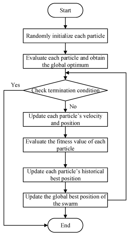
Figure 4. Logical diagram of the PSO algorithm.

The principle of the Deep Neural Network (DNN) is to update its parameters through the backpropagation (BP) algorithm based on gradient descent. BP may suffer from problems such as gradient vanishing or explosion, easy getting trapped in local minima, and strong dependence on hyperparameters such as the learning rate [28]. In order to solve these problems, this study combines Particle Swarm Optimization (PSO) with DNN to form a hybrid Particle Swarm Optimization–Deep Neural Network (PSO-DNN) algorithm. The core idea is to use the PSO algorithm to explore the parameter space and search for the global optimum by iteratively updating the velocity and position of each particle, thereby optimizing the parameters of the DNN to improve training stability, convergence speed, and prediction accuracy [29].

Combining the global optimization capability of PSO with the strong nonlinear fitting ability of DNN, this hybrid algorithm overcomes the problem of DNN easily falling into local optima and reduces the model’s sensitivity to hyperparameters. It effectively alleviates the randomness and instability commonly observed in traditional BP training.

3.3.3. NGO-LSSVM

In 2022, Mohammad et al. proposed the Northern Goshawk Optimization (NGO) algorithm [30], inspired by the predatory behavior of the northern goshawk (Accipiter gentilis). As a recently developed population-based metaheuristic algorithm, NGO demonstrates excellent global search ability, fast convergence speed, and strong robustness.

The search process of NGO consists of two main phases: the prey detection and attack phase (Exploration) and the pursuit and escape phase (Exploitation). In the first phase, each individual simulates the goshawk’s process of locating and identifying its prey in nature, performing global exploration through position interaction with randomly selected “prey” individuals. Specifically, each agent randomly selects another candidate solution $P$ as its prey and updates its position according to their relative distance, which can be expressed as

$$P_i=x_k,i=1,2,\dots ,N,k=1,2,\dots ,i-1,i+1,\dots ,N$$

(7)

$$x_{\mathrm{i},j}^{new,P_1}=\left\{\begin{array}{c}{x}_{i,j}+r\left(p_{i.j}-I{x}_{i,j}\right), F_{P_i}<F_i\\ x_{i,j}+r\left(x_{i.j}-p_{i,j}\right), F_{P_i}\ge F_i\end{array}\right.$$

(8)

$$X_i=\left\{\begin{array}{c}{X}_{\mathrm{i}}^{new,P_1}, F_i^{new,P_1}<F_i\\ X_i, F_i^{new,P_1}\ge F_i\end{array}\right.$$

(9)

where $P_i$ is the position of prey for the $i$th northern goshawk, $F_{P_i}$ is its objective function value, $k$ is a random natural number in interval $\left[1,N\right]$, $X_{\mathrm{i}}^{new,P_1}$ is the new status for the $i$th proposed solution, $x_{\mathrm{i},j}^{new,P_1}$ is its $j$th dimension, $F_i^{new,P_1}$ is its objective function value based on first phase of NGO, $r$ is a random number in interval $\left[0,1\right]$, and $I$ is a random number that can be 1 or 2. Parameters $r$ and $I$ are random numbers used to generate random NGO behavior in search and update.

As the algorithm proceeds to the later iterations, individuals gradually enter the pursuit and escape phase, simulating the high-speed chase of the goshawk and the evasive maneuvers of the prey. This phase focuses on local exploitation to refine the solution accuracy. To control the search range, a dynamic contraction radius $R\left(t\right)$ is introduced, defined as

$$x_{\mathrm{i},j}^{new,P_2}=x_{i,j}+R\left(2r-1\right)x_{i,j}$$

(10)

$$R=0.02\left(1-{\displaystyle \frac{t}{T}}\right)$$

(11)

$$X_i=\left\{\begin{array}{c}{X}_{\mathrm{i}}^{new,P_2}, F_i^{new,P_2}<F_i\\ X_i, F_i^{new,P_2}\ge F_i\end{array}\right.$$

(12)

where $t$ is the iteration counter, $T$ is the maximum number of iterations, $x_{\mathrm{i}}^{new,P_2}$ is the new status for $i$th proposed solution, $x_{\mathrm{i},j}^{new,P_2}$ is its $j$th dimension, $F_i^{new,P_2}$ is its objective function value based on second phase of NGO.

After updating all individuals in both phases, the algorithm evaluates the fitness of each candidate and proceeds to the next iteration. Upon completion, the NGO adopts the best solution obtained throughout the iterations as the final global optimum.

The Least Squares Support Vector Machine (LSSVM) [31] is a variant of the traditional Support Vector Machine (SVM), which transforms the original convex quadratic programming problem into the solution of a set of linear equations, thereby simplifying computation. Its main advantages include high computational efficiency, simple implementation, and good generalization performance. It is also sensitive to model parameters (such as the penalty factor $\gamma$ and the kernel function parameter $\sigma$), and may suffer from overfitting or local optima in certain cases.

Given a set of training samples $\left(x_i,y_i\right),i=1,\dots ,n$, the objective function of LSSVM can be expressed as

$$\underset{w,b,e}{\min }{\displaystyle \frac{1}{2}}{w}^{T}w+{\displaystyle \frac{\gamma }{2}}\sum _{i=1}^n{e}_i^2$$

(13)

subject to

$$y_i=w^T\phi \left(x_i\right)+b+e_i,i=1,\dots ,n$$

(14)

where $\phi \left(\cdot \right)$ is the kernel mapping that projects input data into a high-dimensional feature space, $e_i$ denotes the error term, and $\gamma$ is the regularization (penalty) parameter.

By applying the Lagrange multiplier method, the optimization problem can be converted into a system of linear equations in the following form:

$$\left(\begin{array}{cc}0& 1^T\\ 1& \Omega +{\displaystyle \frac{1}{\gamma }}I\end{array}\right)\left(\begin{array}{c}b\\ \alpha \end{array}\right)=\left(\begin{array}{c}0\\ y\end{array}\right)$$

(15)

where ${\mathsf{\Omega }}_{ij}=K\left(x_i,x_j\right)=\phi {(x_i)}^T\phi \left(x_j\right)$, $\alpha$ is the vector of Lagrange multipliers, and $K\left(\cdot ,\cdot \right)$ denotes the kernel function. The prediction for a new sample $x$ is given by

$$\widehat{y}={\displaystyle \sum }_{i=1}^n{\alpha }_{i}K\left(x_i,x\right)+b$$

(16)

For LSSVM, the penalty parameter $\gamma$ and the kernel parameter $\sigma$ (e.g., the width of the Gaussian kernel) are two crucial hyperparameters that strongly affect model performance. Conventional tuning methods such as grid search, cross-validation, genetic algorithms, or particle swarm optimization can be computationally expensive, prone to local optima, and sensitive to initial values.

To overcome these limitations, this study integrates the Northern Goshawk Optimization (NGO) algorithm with LSSVM, using NGO to optimize the hyperparameters $\gamma$ and $\sigma$. NGO performs global exploration within the parameter space, helping to avoid premature convergence and improving the overall optimization quality.

Therefore, the NGO-LSSVM approach offers several advantages: compared to traditional grid search, NGO allows more flexible and extensive exploration of the search space and has a greater chance of escaping local minima. For complex nonlinear problems, NGO-LSSVM demonstrates superior prediction accuracy and stability. Since LSSVM solves linear equations rather than quadratic programming, the overall model maintains high computational efficiency. Consequently, NGO-LSSVM is well-suited for modeling the broad and nonlinear data characteristics of the afterburning test dataset used in this study.

3.3.4. Comparison of Two Hybrid Algorithms

The two hybrid models exhibit distinct modeling characteristics and limitations. PSO-DNN leverages the strong nonlinear representation capability of neural networks and the global optimization ability of PSO, enabling high-accuracy function approximation in complex engine systems. However, its performance is strongly dependent on hyperparameter tuning, and PSO-based network optimization often incurs substantial computational cost, especially when the search space is large [32].

In contrast, NGO-LSSVM benefits from the convex optimization structure of LSSVM, which ensures faster convergence and better stability under small-sample conditions, while the NGO algorithm enhances global kernel parameter search efficiency [33]. Nevertheless, due to the limited nonlinear mapping capacity of kernel methods, NGO-LSSVM may exhibit reduced predictive fidelity when modeling highly nonlinear interactions compared with deep neural networks.

4. Modeling Process and Experimental Results

4.1. Model Construction and Hyperparameter Configuration

Guided by the aforementioned theoretical foundations of the algorithms, this study carries out specific data modeling and validation work. Based on existing test-bench data, the objective of this research is to characterize the mapping relationship between the inputs and key performance parameters of the light-duty afterburning engine. To reveal the mapping relationship and to achieve quantitative prediction, it is necessary to construct an appropriate regression model to describe and analyze this relationship.

In this study, test-bench data from the TWP220L light-duty afterburning turbojet engine were used as the sample set for analysis. All training samples correspond to independent steady-state engine operating points under varying conditions. Table 1 shows the technical specifications of TWP220L (Institute of Engineering Thermophysics, Chinese Academy of Sciences, Beijing, China).

Table 1. The technical specifications of TWP220L.

Parameters	TWP220L
Thrust (N)	2200
Maximum Length (mm)	1306
Maximum Outer Diameter (mm)	320
Dry Weight (kg)	48

The test cases were taken from ground-based test bench experiments, in which the engine was adjusted to a series of preset steady-state operating points. These operating conditions were generated by artificially varying fuel flow, rotor speed, altitude, and Mach number to cover a typical range of flight conditions. Each operating point was held for several seconds to ensure repeatability, and the measurements were averaged over the stabilization period. Based on the engine’s physical characteristics and experimental data, as shown in Figure 5, Altitude $H$, Mach number $Ma$, rotor speed (rpm) $N$, and fuel flow rate $W_f$ were selected as input variables, while thrust $F$ and turbine pressure ratio ${\pi }_T$ were chosen as output variables.

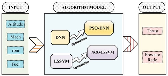
Figure 5. Framework of hybrid algorithm data-driven modeling and optimization.

As listed in Table 2, the input parameters are subject to measurement uncertainties inherent to standard aerospace instrumentation. For instance, the rotor speed ($N$), measured via a magnetic pickup, typically has a high precision of ±0.1%, while the afterburner fuel flow ($W_f$), measured by mass flowmeters, exhibits a relative uncertainty of approximately ±1.0% due to fluid dynamic complexities. These uncertainties are considered as Type B uncertainties in the modeling process.

Table 2. Measurement Parameters and Associated Uncertainties.

Parameter	Symbol	Unit	Measurement Device	Uncertainty
Flight Altitude	$H$	km	Barometric Altimeter	±30 m
Mach Number	$Ma$	-	Air Data Computer	±0.01
Rotor Speed	$N$	r/min	Magnetic Speed Pickup	±0.1% FS
Afterburner Fuel Flow Rate	$W_f$	kg/h	Mass Flowmeter	±1.0%

Modeling and analysis were performed using MATLAB 2022b. The dataset contained 121 steady-state operating points of the TWP220L light afterburning turbojet engine, with a thrust range of [700–2000] N and a turbine pressure ratio range of [1.65–1.85]. The dataset was divided into training and testing sets in a 7:3 ratio, with 85 samples (70.2%) used for training and 36 samples (29.8%) used for testing. Samples were randomly selected to ensure coverage of various operating conditions.

To enhance model generalization and training stability, the dataset was randomly shuffled prior to training to minimize the impact of sample order on the results. Subsequently, all input features were normalized to ensure their values fall within the same magnitude range, thereby preventing large-magnitude features from dominating gradient updates and improving the stability of network training. And the model training incorporated a 5-fold cross-validation setup. The final metrics are averaged across folds to reduce the bias of a single random split.

Figure 6 illustrates the overall process of the data-driven modeling process for the afterburning engine. The experimental dataset is divided into training and testing subsets. The training set is used to construct the algorithmic model and perform hyperparameter optimization to obtain the optimal configuration. Critical hyperparameters were selected based on a combination of literature guidance and preliminary tuning, with optimization algorithms employed to identify values yielding the best performance. The trained model is evaluated on the testing set to verify its predictive accuracy and generalization capability by visual results and regression evaluation metrics.

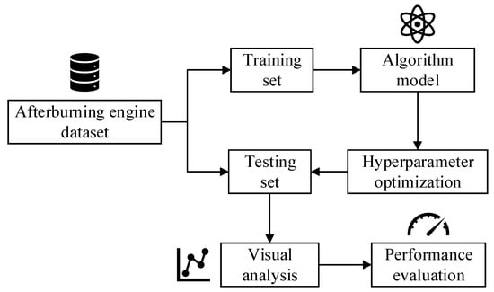
Figure 6. Schematic of the afterburning engine algorithm modeling process.

In this study, the PSO algorithm is first employed to jointly optimize the learning rate and the number of hidden layer nodes. The optimized parameters of the DNN network obtained from PSO are denoted as $l{r}^{\ast }$ (optimal learning rate) and $n{h}^{\ast }$ (optimal number of hidden layer nodes). Table 3 presents the detailed parameter configuration of the PSO-DNN algorithm, including both the PSO parameters and the DNN training settings. The DNN network architecture consists of an input layer with dimensions $\left[f,1,1\right]$, followed by a fully connected layer with 64 nodes and a ReLU activation layer. Subsequently, two fully connected layers are stacked, with the number of nodes in each layer determined by the parameters optimized via the PSO algorithm, and a ReLU activation layer is connected after each fully connected layer.

Table 3. Hyperparameter configuration of the PSO-DNN model.

Category	Parameter	Value/Range
PSO Algorithm Parameters	Population size	6
	Maximum iterations	8
	Optimization dimension	2
	Learning rate range	$lr\in \left[1\times 10-5,1\times 10-1\right]$
	Hidden nodes range	$nh\in \left[5,100\right]$
	Fitness function	@fical
DNN Training Parameters	Optimization algorithm	adam
	Maximum epochs	500
	Initial learning rate	$l{r}^{\ast }$ (Optimized by PSO)

The PSO algorithm in this study uses a population size of 6 and 8 iterations. These values were selected because the hyperparameter search space is low-dimensional and the dataset contains only 121 steady-state samples, which limits the required model complexity. Tests with slightly larger PSO settings showed negligible improvement in prediction accuracy while increasing computation time.

Subsequently, the NGO algorithm was employed to perform global optimization of the key parameters of the LSSVM model, with the corresponding parameter settings summarized in Table 4. In this optimization framework, the kernel function parameter and the penalty parameter were selected as the decision variables, and the objective was to minimize the model’s prediction error. The fitness function, denoted as getObjValue, constitutes the core evaluation component of the optimization process. Specifically, this function assigns each candidate combination of kernel and penalty parameters generated by the NGO algorithm to the LSSVM model and computes the corresponding error score via five-fold cross-validation. The resulting error metric is then fed back to the optimization algorithm to quantitatively assess the quality of the current parameter configuration and guide the subsequent search process.

Table 4. Hyperparameter configuration of the NGO-LSSVM model.

Category	Parameter	Value/Range
NGO Algorithm Parameters	Population size	10
	Maximum iterations	30
	Optimization dimension	2
	Fitness function	@getObjValue
LSSVM Model Parameters	Model type	Regression
	Kernel function	RBF kernel
	Kernel parameter	[0.1, 800]
	Penalty parameter	[0.1, 200]

4.2. Model Simulation and Result Analysis

4.2.1. The Analysis of Thrust Prediction Model

The models for thrust prediction were constructed and fitted, and the results are shown below. Figure 7 presents the performance of the four models on the training set, and Figure 8 illustrates their performance on the test set.

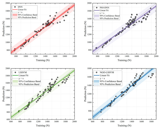
Figure 7. Training results of fitting line of thrust prediction with 4 models.

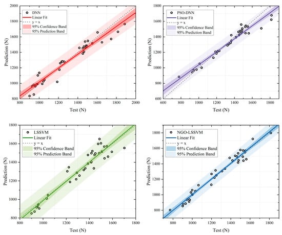
Figure 8. Testing results of fitting line of thrust prediction with 4 models.

The results obtained through training are shown in Figure 7. The plots illustrate the performance of four algorithms in thrust prediction tasks on the training dataset. The horizontal axis represents the actual thrust ($N$), while the vertical axis denotes the predicted thrust ($N$). Black dots indicate the sample data, the colored solid line represents the fitting line, the gray dashed line is the ideal line ($y = x$), the dark-colored region denotes the confidence interval, and the light-colored region indicates the prediction interval. The degree of alignment between the fitting line and the ideal line reflects the consistency between the model’s predicted and actual values.

As shown in Figure 7, all four models exhibit prediction results close to the ideal line, suggesting satisfactory fitting performance. The DNN model (top left) can capture the overall data trend reasonably, but its confidence and prediction bands are relatively wide, indicating greater uncertainty in training predictions. The PSO-DNN model (top right), demonstrates a closer alignment with the ideal line and stronger overall correlation, yet its prediction band remains somewhat broad, indicating that there is still some uncertainty in the prediction.

The LSSVM model (bottom left) achieves a fitting curve that nearly coincides with the ideal line, with narrower confidence and prediction bands, reflecting high fitting accuracy and stability. However, it still exhibits a slight bias in the low thrust region. In contrast, the NGO-LSSVM model (bottom right) shows the best performance among the four. Its fitting line aligns almost perfectly with the ideal line, and both confidence and prediction bands are the narrowest, indicating the lowest prediction error and the strongest generalization capability on the training set.

The NGO-LSSVM achieves the highest coefficient of determination (R²) of 0.97, which is a significant improvement over the 0.90 of the standard DNN model. Moreover, the Root Mean Square Error (RMSE) is reduced from 37.42 N to 47.29 N. Crucially, the 95% confidence band (represented by the shaded area) in NGO-LSSVM is noticeably narrower than that in DNN. And 96.5% of the test data points strictly fall within this prediction interval. This demonstrates that the proposed hybrid strategy not only improves accuracy but also significantly reduces the epistemic uncertainty of the model. In summary, the NGO-LSSVM model demonstrates the best training performance in thrust prediction on the training set.

The data distribution trend of the DNN model is similar to that of the training set, remaining relatively dispersed. The fitting line deviates to some extent from the ideal line, and the confidence interval is relatively wide, indicating that the model’s generalization performance is moderate. The deviation of several data points from the main diagonal further suggests that the DNN’s ability to capture feature representations is still limited.

Compared with DNN, the PSO-DNN model shows a larger deviation between the fitting line and the ideal line, but its data distribution is more concentrated and the confidence interval is significantly narrower. This indicates a clear improvement in predictive capability. It demonstrates that PSO-DNN effectively avoids the local minima problem of gradient descent, improving prediction accuracy and stability. The deviation of its fitting line also implies that the model still exhibits a certain degree of overfitting.

For the LSSVM model, the fitting line is very close to the ideal line, but the overall data distribution remains scattered, reflected in its wide prediction interval. The relatively dispersed distribution of data points indicates limited generalization capability on the test set. This phenomenon mainly arises from the model’s sensitivity to kernel parameters and its limited ability to capture strong nonlinear characteristics of thrust.

Quantitatively, as listed in Table 5, the NGO-LSSVM achieves a coefficient of determination (R²) of 0.94, which represents a significant improvement over the 0.83 of the baseline DNN model and the 0.89 of the standard LSSVM. Furthermore, the Mean Squared Error (MSE), which penalizes larger prediction deviations, is reduced to 4698.83 for the NGO-LSSVM. In contrast, the PSO-DNN model yields a much higher MSE of 8559.37, indicating that while the particle swarm optimization improved some local predictions, it failed to suppress large error spikes effectively. The prediction band width of the hybrid algorithm is reduced by approximately 30% compared to traditional algorithms. The 95% confidence band is visibly narrower compared to the DNN and the LSSVM, confirming that the NGO-LSSVM significantly reduces the epistemic uncertainty of the thrust prediction.

Table 5. Regression evaluation metrics of four models for thrust prediction.

	DNN	PSO-DNN	LSSVM	NGO-LSSVM
R2	0.83	0.87	0.89	0.94
MAE	58.25	53.33	55.03	54.73
MSE	6237.06	8559.37	5222.74	4698.83
MAPE	0.039	0.036	0.044	0.034

In summary, the DNN model effectively represents nonlinear relationships but is sensitive to initial parameters. PSO-DNN improves convergence and fitting ability through swarm intelligence optimization. LSSVM performs well overall but exhibits scattered data points. And NGO-LSSVM, by combining the optimization algorithm with kernel-based learning, achieves the best prediction accuracy and generalization performance among the four models.

4.2.2. The Analysis of Pressure Ratio Prediction Model

Figure 9, Figure 10, Figure 11 and Figure 12 illustrate the error distributions of four models in pressure ratio prediction. Figure 9 and Figure 10 correspond to the training set, while Figure 11 and Figure 12 show the testing set.

Figure 9. Training results of error distributions for pressure ratio prediction with 4 models.

Figure 10. Training results of spiral graph of absolute errors in pressure ratio prediction across 4 models.

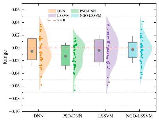
Figure 11. Testing results of error distributions for pressure ratio prediction with 4 models.

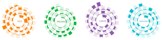
Figure 12. Testing results of spiral graph of absolute errors in pressure ratio prediction across 4 models.

Figure 9 and Figure 10 illustrate the error distribution characteristics of four models for pressure ratio prediction. Figure 9 uses box plots and scatter plots to show the training error distribution (true value minus predicted value), reflecting the overall dispersion of each model. Figure 10 visually displays the absolute error of each data point in the form of a spiral graph, with the height of the darker blocks representing the magnitude of the error. The color gradient is calibrated such that light-colored shading represents a relative error rate within the 5% margin, while darker segments indicate errors exceeding this threshold.

As shown in Figure 9, the error distributions of the four models are quite different. It can be observed that there are significant differences in the dispersion and shape of the error distribution. The DNN model’s error distribution is relatively dispersed, with multiple extreme outliers, and the box center point deviates from the zero-error line, indicating that its fit on some samples is unstable. By comparison, the PSO-DNN model has a narrower box range and fewer outliers, indicating stronger training robustness, but its box center still deviates from the zero-error line. The LSSVM model’s box center point is close to the zero-error line, but the overall box is relatively wide, indicating that the prediction accuracy is still insufficient.

In contrast, the NGO-LSSVM model achieves the most compact distribution, with a well-positioned box center coinciding with the zero-error line and the narrowest overall box, demonstrating better prediction accuracy and stability in pressure ratio modeling. The NGO-LSSVM achieves a Mean Absolute Percentage Error (MAPE) of 0.82%. This is a substantial improvement over the DNN (0.93%) and PSO-DNN (0.88%) models. While the R² values for pressure ratio are generally lower than those for thrust due to the compound nature of the parameter, the NGO-LSSVM still maintains the highest score of 0.80, compared to 0.73 for the DNN.

Figure 10 shows the spiral distribution of the absolute error. It can be seen that DNN and LSSVM have several blocks that extend beyond the acceptable range, indicating the presence of several extreme errors. The DNN and PSO-DNN models display distinct dark orange and green bands in the outer rings, corresponding to the Mean Absolute Error (MAE) of 0.017 and 0.015, respectively. Compared to DNN and LSSVM, PSO-DNN and NGO-LSSVM produce smaller and more uniform errors, demonstrating that the optimization algorithms effectively enhance the model’s generalization ability and reduce local bias. In contrast, the NGO-LSSVM spiral is dominated by light blue segments, reflecting a lower MAE of 0.013. This corresponds to the lowest MSE of 0.00033 among all comparisons. NGO-LSSVM exhibits the smallest overall fluctuation in absolute error, but the difference compared to other algorithms is not significant, requiring further observation in the test set prediction results.

In summary, the NGO-LSSVM model demonstrates the most concentrated and stable error behavior in pressure ratio prediction. These results indicate that the NGO effectively enhances the model’s global search and parameter generalization capabilities, leading to improved accuracy and robustness in complex nonlinear regression tasks.

Figure 11 and Figure 12 present the error distribution characteristics of four models on the testing dataset for pressure ratio prediction. The parameter representations in the figures are the same as in Figure 9 and Figure 10, and will not be repeated here.

As shown in Figure 11, these models exhibit noticeable differences in their testing performance compared with the training results. The DNN and LSSVM models have large bin sizes, with the DNN bin center point deviating significantly from the zero-error line, indicating poor prediction stability on unseen samples. The PSO-DNN model has a narrower error range but several extreme negative biases, causing the bin center point to deviate severely from the zero-error line, suggesting potential underfitting in certain regions. The NGO-LSSVM model has a more concentrated error distribution, fewer biases, a center point close to the zero-error line, and the narrowest bin length, with only a few outliers, indicating superior generalization accuracy and more stable prediction performance.

Numerical results confirm this visual observation. The NGO-LSSVM achieves a Mean Absolute Percentage Error (MAPE) of 0.97% (0.0097). This is a substantial improvement over the DNN (1.2%) and PSO-DNN (1.2%) models. While the R² values for pressure ratio are generally lower than those for thrust due to the compound nature of the parameter, the NGO-LSSVM still maintains the highest score of 0.73, compared to 0.63 for the DNN. The NGO-LSSVM result of <1% MAPE indicates that the hybrid kernel method possesses stronger robustness against measurement fluctuations.

Figure 12 shows the spiral distribution of the absolute errors of the four models on the test set. The DNN model still exhibits several relatively large error blocks, while the distribution of smaller error blocks is also relatively dense. The DNN and PSO-DNN models display multiple distinct dark bands in the outer rings, revealing that a notable portion of predictions suffer from errors larger than 5%, particularly during rapid transient phases. It is worth noting that although PSO-DNN shows a good distribution in the spiral plot and has no extreme error values, its box plot deviates significantly from the zero-error line, indicating that while the model’s predictions are stable across the entire data range, it exhibits systematic overestimation. LSSVM performs similarly to DNN, exhibiting some extreme error values and significant error fluctuations. In sharp contrast, the spiral of the NGO-LSSVM model is predominantly covered by light shading. This visual dominance confirms that the vast majority of the prediction results are constrained within the 5% error bound.

In summary, the NGO-LSSVM model achieves the most concentrated and stable error distribution on the test dataset, demonstrating excellent generalization performance. These results confirm that the NGO algorithm can effectively enhance the predictive power of LSSVM, improve its reliability for unseen data, and provide a more accurate framework for aero-engine performance modeling.

4.2.3. The Analysis of Regression Evaluation Metrics

To further quantify the overall performance differences among the four models in thrust and pressure ratio prediction, in addition to visualization analysis, this study also employed regression evaluation metrics on the test dataset. The accuracy, stability, and generalization ability of each model were comprehensively assessed by calculating the coefficient of determination (R²), mean absolute error (MAE), mean squared error (MSE), and mean absolute percentage error (MAPE).

$$R^2=1-{\displaystyle \frac{{\sum }_{i=1}^n{(y_i-{\widehat{y}}_i)}^2}{{\sum }_{i=1}^n{(y_i-\hat{y})}^2}}$$

(17)

$$MAE={\displaystyle \frac{1}{n}}\sum _{i=1}^n\left|y_i-{\widehat{y}}_i\right|$$

(18)

$$MSE={\displaystyle \frac{1}{n}}\sum _{i=1}^n{(y_i-{\widehat{y}}_i)}^2$$

(19)

$$MAPE={\displaystyle \frac{100\%}{n}}\sum _{i=1}^n\left|{\displaystyle \frac{y_i-{\widehat{y}}_i}{y_i}}\right|$$

(20)

where $y_i$ represents true value, ${\widehat{y}}_i$ represents predicted value, $\overline{y}={\displaystyle \frac{1}{n}}{\sum }_{i=1}^n{y}_i$ represents the true values. Since all data are strictly positive and do not approach zero, MAPE can be reliably applied without risk of division-by-zero or inflated values.

Table 5 and Table 6 present the regression evaluation metrics of four models on thrust and pressure ratio prediction tasks of the test set, respectively. Similar evaluation metrics have been used in recent aero-engine prediction studies. For example, Deng and Zhou [34] employed a CNN–LSTM–Attention model on the CMAPSS dataset and reported RMSE values in the range of approximately 14–16. Jin et al. [35] proposed a power-based self-tuning model which significantly reduced MAE and RMSE in aero-engine gas-path prediction tasks. He et al. [36] proposed the SA-CNN-BiLSTM hybrid network for remaining useful life (RUL) prediction, which can be used for comparison using RMSE/MAE metrics. These studies collectively confirm the suitability of R², MAE, MSE, and RMSE as performance evaluation metrics and their consistency with current research practices.

Table 6. Regression evaluation metrics of four models for pressure ratio prediction.

	DNN	PSO-DNN	LSSVM	NGO-LSSVM
R2	0.63	0.70	0.68	0.73
MAE	0.020	0.021	0.020	0.017
MSE	0.00067	0.00071	0.00059	0.00048
MAPE	0.012	0.012	0.011	0.0097

For thrust prediction, shown in Table 5, all models achieve relatively high R² values (R² > 0.8), indicating strong fitting capability. Among them, NGO-LSSVM exhibits the best overall performance, with the highest coefficient of determination (R² = 0.94) and the lowest mean square error (MSE = 4698.83). This demonstrates that the integration of the NGO algorithm effectively enhances the nonlinear fitting ability of LSSVM and improves generalization. Although PSO-DNN achieves a slightly lower R², its mean absolute error (MAE = 53.33) and mean absolute percentage error (MAPE = 0.036) remain competitive, suggesting that particle swarm optimization contributes to local convergence improvement but still suffers from potential overfitting. In contrast, the plain DNN model shows the weakest performance, confirming that simple neural architectures are insufficient to capture the complex coupling relationships in the afterburning process.

For pressure ratio prediction, shown in Table 6, the performance differences among models are less pronounced, and the R² values are generally lower (ranging from 0.66 to 0.73), indicating that pressure ratio prediction is more difficult due to stronger parameter coupling and narrower value range. The lower R² values for pressure ratio prediction are likely due to its small variance and narrow operational range, making its prediction more sensitive to measurement noise and minor input variations. Even so, NGO-LSSVM again achieves the lowest errors (MAE = 0.017, MSE = 0.00048, MAPE = 0.0097), demonstrating better robustness and accuracy. Other models perform relatively worse, suggesting that purely data-driven deep models are less effective when the mapping is weakly nonlinear and data size is limited.

In summary, the NGO-LSSVM model achieves superior fitting accuracy and generalization across both prediction tasks, verifying the effectiveness of combining a kernel-based regression model with an intelligent optimization algorithm.

5. Conclusions

In this study, a data-driven hybrid algorithm modeling approach for light-duty afterburning turbojet engines is proposed, which integrates metaheuristic global search and statistical/connectionist regressors to overcome strong nonlinearity and multivariate coupling problems. Using test-bench data, PSO-DNN and NGO-LSSVM are instantiated to map engine inputs (Altitude, Mach number, rotor speed, fuel flow rate) to thrust and turbine total pressure ratio. Combining fitting diagnosis, confidence/prediction band analysis, spiral absolute error visualization, and R²/MAE/MSE/MAPE regression evaluation metrics, it was found that NGO-LSSVM consistently achieves the highest accuracy and stability, especially on the test set data. This advantage is particularly evident in thrust prediction, where NGO-LSSVM attains the largest R² and the lowest overall error levels, confirming that the integration of the NGO algorithm significantly enhances the nonlinear fitting capability and generalization performance of LSSVM. Although PSO-DNN improves convergence behavior and reduces sensitivity to initialization compared with the ordinary DNN, its accuracy and robustness remain inferior to NGO-LSSVM. For the pressure ratio prediction, NGO-LSSVM still maintains the lowest errors among all models, demonstrating its superior adaptability under weakly nonlinear and narrow-range mapping conditions.

These results substantiate that (i) kernel methods endowed with globally optimized hyperparameters provide superior bias–variance trade-offs under limited datasets and tight output ranges, and (ii) swarm-based parameter search effectively mitigates local minima and training stochasticity in deep models. Practically, this model furnishes reliable performance predictors suitable for integration into onboard estimation and control pipelines, including model-predictive and gain-scheduling strategies. Methodologically, the framework is extensible to broader propulsion states (e.g., transient mode transitions) and multimodal sensing, and amenable to uncertainty quantification. Considering these findings, several recommendations for future studies can be outlined. First, closed-loop co-design of the predictor with real-time control laws should be explored to evaluate system-level benefits under operational constraints. Second, domain-shift robustness across expanded flight envelopes and environmental conditions should be systematically assessed, potentially through transfer learning or adaptive updating mechanisms. Third, incorporating physics-guided constraints or hybrid mechanistic–data-driven structures may further enhance interpretability, safety assurance, and real-time deployment capability. These directions would strengthen the applicability of the proposed methodology for next-generation intelligent propulsion systems.

References

- Zhang, X.; Zhang, Y.; Liu, T. Summary of Advanced Afterburner Design Technology. Aeroengine 2014, 40, 24–30. [Google Scholar]
- Liu, J.; Liu, Z. Conceptual Design and Research of Supersonic Target Drone. J. Astronaut. Metrol. Meas. 2016, 36, 60–63, 67. [Google Scholar]
- Li, H.; Feng, G.; Haung, J.; Long, J. Development Review of Aerial Target in China and Abroad. Mod. Def. Technol. 2025, 53, 1–10. [Google Scholar]
- Wang, P.; Cui, L.; Zhang, H. Numerical Study on Performance of Aviation Gas Turbine Engine Based on Component Method. Heilongjiang Sci. 2020, 11, 26–28+31. [Google Scholar]
- Pan, M.; Chen, Q.; Zhou, Y. A multi-dynamics approach to turbofan engine modeling. Acta Aeronaut. Astronaut. Sin. 2019, 40, 99–110. [Google Scholar]
- Shi, R.; Zhou, J.; Zhang, Q. Modeling of whole processes of mixing exhaust afterburner twin spool turbofan engine. J. Aerosp. Power 2013, 28, 2384–2390. [Google Scholar]
- Xia, F.; Huang, J.; Zhou, W. Modeling of and simulation research on turbofan engine based on MATLAB/SIMULINK. Heilongjiang Sci. 2007, 22, 2134–2138. [Google Scholar]
- Li, J.; Zhou, D.; Xiao, W.; Zhang, H. Hybrid Modeling of Gas Turbine based on Neural Network. J. Eng. Therm. Energy Power 2019, 34, 33–39. [Google Scholar]
- Keshun, Y.; Guangqi, Q.; Yingkui, G. A 3-D Attention-Enhanced Hybrid Neural Network for Turbofan Engine Remaining Life Prediction Using CNN and BiLSTM Models. IEEE Sens. J. 2024, 24, 21893–21905. [Google Scholar] [CrossRef]
- Zhao, Y.; Li, Z.; Hu, Q. A size-transferring radial basis function network for aero-engine thrust estimation. Eng. Appl. Artif. Intell. 2020, 87, 103253. [Google Scholar] [CrossRef]
- Alozie, O.; Li, Y.-G.; Wu, X.; Shong, X.; Ren, W. An Adaptive Model-Based Framework for Prognostics of Gas Path Faults in Aircraft Gas Turbine Engines. Int. J. Progn. Health Manag. 2019, 10, 13. [Google Scholar] [CrossRef]
- Xue, F.; Jin, G.; Tan, L.; Zhang, C.; Yu, Y. Predictive maintenance programs for aircraft engines based on remaining useful life prediction. Sci. Rep. 2025, 15, 41756. [Google Scholar] [CrossRef]
- Muneer, A.; Taib, S.M.; Fati, S.M.; Alhussian, H. Deep-Learning Based Prognosis Approach for Remaining Useful Life Prediction of Turbofan Engine. Symmetry 2021, 13, 1861. [Google Scholar] [CrossRef]
- Liu, Z.; Karimi, I.A. Gas turbine performance prediction via machine learning. Energy 2020, 192, 116627. [Google Scholar] [CrossRef]
- Gao, W.; Zhou, X.; Pan, M.; Zhou, W.; Lu, F.; Huang, J. Acceleration control strategy for aero-engines based on model-free deep reinforcement learning method. Aerosp. Sci. Technol. 2022, 120, 107248. [Google Scholar] [CrossRef]
- Zheng, Q.; Fang, J.; Hu, Z.; Zhang, H. Aero-Engine On-Board Model Based on Batch Normalize Deep Neural Network. IEEE Access 2019, 7, 54855–54862. [Google Scholar] [CrossRef]
- Harris, J.; Arthurs, F.; Henrickson, J.V.; Valasek, J. Aircraft System Identification Using Artificial Neural Networks With Flight Test Data. In Proceedings of the 2016 International Conference on Unmanned Aircraft Systems (ICUAS), Arlington, VA, USA, 7–10 June 2016; IEEE: New York, NY, USA, 2016. [Google Scholar]
- Du, D.; Jia, X.; Hao, C. A New Least Squares Support Vector Machines Ensemble Model for Aero-Engine Performance Parameter Chaotic Prediction. Math. Probl. Eng. 2016, 2016, 4615903. [Google Scholar] [CrossRef]
- Haung, Y.; Tao, J.; Sun, G. A Novel Digital Twin Approach Based on Deep Multimodal Information Fusion for Aero-Engine Fault Diagnosis. Energy 2023, 270, 126894. [Google Scholar] [CrossRef]
- Loboda, I.; Ruíz, J.L.P.; Castillo, I.G. Simplified Data-Driven Models for Gas Turbine Diagnostics. Machines 2025, 13, 344. [Google Scholar] [CrossRef]
- Lv, C.; Chang, J.; Bao, W.; Yu, D. Recent research progress on airbreathing aero-engine control algorithm. Propuls. Power Res. 2022, 11, 1–57. [Google Scholar] [CrossRef]
- Ma, M.; Jin, J.; Ji, H. Technology and New Configuration of Aero-engine Afterburner. Gas Turbine Exp. Res. 2008, 21, 55–59. [Google Scholar]
- Berberich, J.; Köhler, J.; Müller, M.A.; Allgöwer, F. Data-Driven Model Predictive Control With Stability and Robustness Guarantees. IEEE Trans. Autom. Control 2021, 66, 1702–1717. [Google Scholar] [CrossRef]
- Noori, F.; Gorji, M.; Kazemi, A.; Nemati, H. Thermodynamic optimization of ideal turbojet with afterburner engines using non-dominated sorting genetic algorithm II. Proc. Inst. Mech. Eng. Part G J. Aerosp. Eng. 2010, 224, 1285–1296. [Google Scholar] [CrossRef]
- Lian, X.; Wu, H. Aero Engine Principles; Northwestern Polytechnical University Press: Xi’an, China, 2005. [Google Scholar]
- Kennedy, J.; Eberhart, R. Particle swarm optimization. In Proceedings of the ICNN’95—International Conference on Neural Networks, Perth, WA, Australia, 27 November–1 December 1995; IEEE: New York, NY, USA, 1995; Volume 4, pp. 1942–1948. [Google Scholar]
- Shami, T.M.; El-Saleh, A.A.; Alswaitti, M.; Al-Tashi, Q.; Summakieh, M.A.; Mirjalili, S. Particle Swarm Optimization: A Comprehensive Survey. IEEE Access 2022, 10, 10031–10061. [Google Scholar] [CrossRef]
- Liu, X.; He, P.; Chen, W.; Gao, J. Multi-Task Deep Neural Networks for Natural Language Understanding. In Proceedings of the 57th Annual Meeting of the Association for Computational Linguistics; IEEE: New York, NY, USA, 2019; pp. 4487–4496. [Google Scholar]
- Koessler, E.; Almomani, A. Hybrid particle swarm optimization and pattern search algorithm. Optim. Eng. 2021, 22, 1539–1555. [Google Scholar] [CrossRef]
- Dehghani, M.; Hubálovský, Š.; Trojovský, P. Northern Goshawk Optimization: A New Swarm-Based Algorithm for Solving Optimization Problems. IEEE Access 2021, 9, 162059–162080. [Google Scholar] [CrossRef]
- Wei, M.; Wang, X.; Fu, Y.; Wang, D.; Li, Y. A Review of LSSVM Mathematical Models and Applications. In Proceedings of the 2024 5th International Conference on Mechatronics Technology and Intelligent Manufacturing (ICMTIM), Nanjing, China, 26–28 April 2024. [Google Scholar]
- Kaya, U.; Yılmaz, A.; Aşar, S. Sepsis Prediction by Using a Hybrid Metaheuristic Algorithm: A Novel Approach for Optimizing Deep Neural Networks. Diagnostics 2023, 13, 2023. [Google Scholar] [CrossRef]
- Shen, Y.; Fu, L. Sensor dynamic modelling based on NGO-LSSVM. In Proceedings of the Fifth International Conference on Control, Robotics, and Intelligent System (CCRIS 2024), Macau, China, 23–25 August 2024; Volume 13404. [Google Scholar]
- Deng, S.; Zhou, J. Prediction of Remaining Useful Life of Aero-engines Based on CNN-LSTM-Attention. Int. J. Comput. Intell. Syst. 2024, 17, 232. [Google Scholar] [CrossRef]
- Jin, Z.; Ouyang, T.; Liu, J.; Suo, S.; Xu, M.; Song, Z. Power-based self-tuning model for aero-engine using MLP-assisted inverse control with filtered error feedback. Aerosp. Sci. Technol. 2025, 168, 110927. [Google Scholar] [CrossRef]
- He, Y.; Wen, C.; Xu, W. Residual Life Prediction of SA-CNN-BILSTM Aero-Engine Based on a Multichannel Hybrid Network. Appl. Sci. 2025, 15, 966. [Google Scholar] [CrossRef]
Disclaimer/Publisher’s Note: The statements, opinions and data contained in all publications are solely those of the individual author(s) and contributor(s) and not of MDPI and/or the editor(s). MDPI and/or the editor(s) disclaim responsibility for any injury to people or property resulting from any ideas, methods, instructions or products referred to in the content. |
© 2025 by the authors. Licensee MDPI, Basel, Switzerland. This article is an open access article distributed under the terms and conditions of the Creative Commons Attribution (CC BY) license.