Real-Time Trajectory Prediction for Rocket-Powered Vehicle Based on Domain Knowledge and Deep Neural Networks

Abstract

The large-scale trajectory simulation serves as a fundamental basis for the mission planning of a rocket-powered vehicle swarm. However, the traditional flight trajectory calculation method for a rocket-powered vehicle, which employs strict dynamic and kinematic models, often struggles to meet the temporal requirements of mission planning. To address the challenges of timely computation and intelligent optimization, a segmented training strategy, derived from the domain knowledge of the multi-stage flight characteristics of a rocket-powered vehicle, is integrated into the deep neural network (DNN) method. A high-precision trajectory prediction model that fuses multi-DNN is proposed, which can rapidly generate high-precision trajectory data without depending on accurate dynamic models. Based on the determination of the characteristic parameters derived from rocket-powered trajectory theory, a homemade dataset is constructed through a traditional computation method and utilized to train the DNN model. Extensive and varying numerical simulations are given to substantiate the predictive accuracy, adaptability, and stability of the proposed DNN-based method, and the corresponding comparative tests further demonstrate the effectiveness of the segmented strategy. Additionally, the real-time computational capability is also confirmed by computing the simulation of generating full trajectory data.

1. Introduction

The trajectory computation serves as the foundation for the mission planning and decision-making (MPDM) process of the rocket-powered vehicle swarm, as the trajectory simulation can validate the outcomes of MPDM to enhance the success rate of missions. Due to the real-time demands of the MPDM of rocket-powered vehicle swarm, the promptness of trajectory computation becomes an increasingly crucial consideration. Therefore, within this context, the process of MPDM poses a new challenge for the real-time computation of trajectories for rocket-powered vehicle swarm.

Based on existing research, the trajectory prediction problem can be classified into two types by different perspectives: predicting the trajectory of the own flight vehicle and predicting the trajectory of the target flight vehicle. The former typically involves seeking the optimal trajectory for a flight vehicle under certain constraints. The latter, however, aims to predict the future trajectory within a specific time frame based on the historical trajectory of the target, achieving the purpose of intent recognition. Although this research delves into the trajectory prediction of the own flight vehicle, certain theoretical methods from both categories can be mutually beneficial. Therefore, a summary of the related research of both will be developed next.

For target flight vehicle trajectory prediction, there are currently two main methods. One method is based on the principle of the Kalman filter (KF). This theoretical approach can be used to predict the future state parameters under the constraints of known target vehicle parameters, Gaussian white noise distribution, and associated measurement noise. However, due to the diversity of target vehicle maneuvers, KF methods based on a single dynamical model often struggle to predict accurately. Thus, methods like multi-model filtering [1,2,3] and unscented Kalman filtering [4,5,6] have been proposed to address this issue. The other approach is based on deep learning. In order to overcome the inability of traditional filtering methods to adapt to the varying model, numerous scholars have explored deep neural networks (DNNs) for model-free trajectory prediction. Considering the temporal characteristics of trajectory data, the recurrent neural network represented by long short-term memory (LSTM) has been widely used to train trajectory prediction models. D. Lui designed two distinct model architectures using LSTM, trained with significant offline real trajectory data to predict the positions and velocities of the flight vehicle from raw radar measurement data, and compared their predictions against the interactive multiple model, concluding that data-driven models have good generalization capabilities [7]. Similar work has been done in [8,9,10].

The methods for predicting the trajectory of the own flight vehicle are also mainly classified into two categories. One type includes traditional analytical methods and numerical integration methods. In the works of [11,12,13,14,15,16], the analytic solution of the glide trajectory for a hypersonic vehicle is derived by a perturbation method and spectral decomposition method. The accuracy of the analytical solution depends on the accuracy and complexity of the model, and thus the derivation process of analytical solutions is often extremely complicated, and the accuracy of results is difficult to guarantee. The numerical integration method is different from the analytical method. Although the high accuracy of its calculation results can be guaranteed, it requires a large amount of computation and a long computation time. The common numerical integration methods include the Runge–Kutta methods and so on. In addition, some intelligent optimization algorithms have been combined to rapidly solve the rocket-powered trajectory parameters. Wei et al. [17] numerically solved trajectory parameters through polynomial fitting and the Levenberg–Marquardt (L-M) search method. Furthermore, in the work of [18], a method combining the BP neural network and L-M algorithm was proposed to achieve the accurate and fast computation of a rocket-powered trajectory. In this method, the BP neural network is used to quickly predict the initial values of the rocket-powered trajectory parameters, and the L-M algorithm is used for further numerical optimization calculation. Based on the high efficiency of gradient search and the stochastic nature of particle swarm search, a hybrid particle swarm algorithm was proposed for the optimization calculation of the rendez-vous trajectory of the ascent section of a launch vehicle [19]. The second category involves DNN-based approaches. Taking advantage of the excellent fitting ability of neural networks to nonlinear models, researchers have applied them to fit and approximate missile trajectories for rapid prediction. Dong et al. [20] utilized BP neural networks to fit the coefficients of missile trajectory equations to rapidly generate trajectory curves, but in this method, the predictive accuracy remains constrained by the precision of the equations, failing to fully leverage the excellent fitting capability of the neural network. Wang et al. [21] developed a neural network structure with two hidden layers, trained on traditional model-generated trajectory data. In this way, the fast prediction of rocket-powered trajectories can be realized within a small error margin and its solving time is only one-fourth of the traditional iterative calculation algorithms. Wang et al. [22] used the optimal trajectory data obtained through pseudo-spectral methods to train deep neural networks, obtaining optimal trajectory neural network models. Compared to traditional methods, this approach not only meets accuracy requirements but also exhibits good generalization. Similar works using DNN-based onboard controllers for real-time optimization control include [23,24]. In addition, there have been preliminary DNN-based algorithms developed to solve the problem of precise landing [25,26,27] and the orbit transfer of spacecraft [28,29,30,31].

Leveraging the strong generalization ability of deep learning methods and the inherent efficiency of matrix-based computation, many studies have developed DNN-based approaches to enable onboard applications that meet real-time computing requirements [22,23,31,32]. In this study, building on the success of deep learning techniques in rapidly generating optimal control solutions, this paper proposes a real-time trajectory rapid computation method based on deep neural networks for rocket-powered vehicles. This method ensures high accuracy while achieving the millisecond-level rapid computation of trajectory, and compared to traditional iterative calculation methods, it better meets the real-time requirements of MPDM for rocket-powered vehicles. Moreover, the model in [21,22] exhibits predictive errors in the kilometer range in the three-dimensional direction, whereas the predictive accuracy of the model in this paper is superior, with average errors within the hundred-meter range. The DNN-based trajectory prediction model obtained in this paper takes the starting and target positions of rocket-powered vehicles as input and outputs three-dimensional trajectory scatter data with a time sequence. The main contributions of this paper are in two aspects:

• To fully leverage the advantages of deep neural networks (DNNs), this paper proposes a technical framework based on the segmented trajectory characteristics of rocket-powered vehicles, consisting of data generation and segmentation, segmented training, and multi-model fusion prediction. Monte Carlo simulation experiments were conducted on the final trajectory generator, confirming the effectiveness of the proposed approach.
• To support the practical training of the proposed DNN-based framework, trajectory data is generated using the traditional iterative calculation method. In order to ensure that the dataset covers arbitrary launch conditions within the national territory, characteristic parameters for trajectory computation are determined based on trajectory principles, allowing for effective range definition and gridding. Additionally, the data is segmented in accordance with the phase-based training strategy, while ensuring logical consistency across different trajectory segments.

Overall, this research effectively addresses the main point that the calculation time of the traditional method is incapable of meeting real-time decision making and rapid response needs for flight vehicles, bearing significant engineering significance.

The rest of the paper is arranged as follows. Section 2 describes the problem and the research idea. Section 3 details the creation of the dataset and the implementation of the segmentation strategy. Section 4 describes the process of determining the neural network structure and training hyperparameters, and obtains the relevant neural network model. Section 5 describes the multi-scaled neural network model cooperation strategy and performs the associated numerical simulations, evaluating the performance of the DNN-based trajectory prediction model. The main work of this paper is summarized in Section 6.

2. Problem Formulation and Research Approach

2.1. The Center-of-Mass Dynamics Model in the Ground-Based Launch Coordinate System

The forces acting on the rocket-powered vehicle are as follows:

$${\mathit{F}}_s=\mathit{mg}+\mathit{R}+{\mathit{P}}_{st}+{\mathit{F}}_c+{\mathit{F}}_k^{\prime }$$

(1)

where $\mathit{mg}$ is the gravitational force vector acting on the rocket, $\mathit{R}$ is the aerodynamic force vector, ${\mathit{P}}_{st}$ is the static component of the engine thrust vector, ${\mathit{F}}_c$ is the control force vector acting on the rocket, and ${\mathit{F}}_k^{\prime }$ is the additional Coriolis force term.

The vector form of the center-of-mass dynamics equation for the rocket-powered vehicle in the inertial coordinate system can then be expressed as

$$m{\displaystyle \frac{{\mathrm{d}}^2\mathit{r}}{\mathrm{d}{t}^2}}=\mathit{P}+\mathit{R}+{\mathit{F}}_c+\mathit{mg}+{\mathit{F}}_k^{\prime }$$

(2)

The differential equations are projected onto the ground-based launch coordinate system for a solution, which is defined on a biaxial rotating ellipsoid that models the Earth as rotating with an angular velocity ${\mathit{\omega }}_e$. According to the vector derivative rule, we obtain

$$m{\displaystyle \frac{{\mathrm{d}}^2\mathit{r}}{\mathrm{d}{t}^2}}=m{\displaystyle \frac{{\delta }^2\mathit{r}}{\delta t^2}}+2m{\mathit{\omega }}_e\times {\displaystyle \frac{\delta \mathit{r}}{\delta t}}+m{\mathit{\omega }}_e\times ({\mathit{\omega }}_e\times \mathit{r})$$

(3)

Substituting this into (2) and rearranging, we obtain

$$m{\displaystyle \frac{{\delta }^2\mathit{r}}{\delta t^2}}=\mathit{P}+\mathit{R}+{\mathit{F}}_c+\mathit{mg}+{\mathit{F}}_k^{\prime }-m{\displaystyle \frac{{\delta }^2\mathit{r}}{\delta t^2}}-2m{\mathit{\omega }}_e\times {\displaystyle \frac{\delta \mathit{r}}{\delta t}}-m{\mathit{\omega }}_e\times ({\mathit{\omega }}_e\times \mathit{r})$$

(4)

Decomposing each term of the above equation in the ground-based launch coordinate system, we obtain

$$\begin{array}{cc}\hfill m\left[\begin{array}{c}{\displaystyle \frac{\mathrm{d}{v}_x}{dt}}\\ {\displaystyle \frac{\mathrm{d}{v}_y}{dt}}\\ {\displaystyle \frac{\mathrm{d}{v}_z}{dt}}\end{array}\right]& ={\mathit{G}}_B\left[\begin{array}{c}P-X_c\\ Y_c+Y_k\\ Z_c-Z_k\end{array}\right]+{\mathit{G}}_V\left[\begin{array}{c}-X\\ Y\\ Z\end{array}\right]+m{\displaystyle \frac{{g^{\prime }}_r}{r}}\left[\begin{array}{c}x+R_{0x}\\ y+R_{0y}\\ z+R_{0z}\end{array}\right]+\hfill \\ \hfill & m{\displaystyle \frac{g_{\omega e}}{{\omega }_e}}\left[\begin{array}{c}{\omega }_{ex}\\ {\omega }_{ey}\\ {\omega }_{ez}\end{array}\right]-m\left[\begin{array}{ccc}{\omega }_{ex}^2-{\omega }_e^2& {\omega }_{ex}{\omega }_{ey}& {\omega }_{ez}{\omega }_{ex}\\ {\omega }_{ex}{\omega }_{ey}& {\omega }_{ey}^2-{\omega }_e^2& {\omega }_{ey}{\omega }_{ez}\\ {\omega }_{ez}{\omega }_{ex}& {\omega }_{ey}{\omega }_{ez}& {\omega }_{ez}^2-{\omega }_e^2\end{array}\right]\left[\begin{array}{c}x+R_{0x}\\ y+R_{0y}\\ z+R_{0z}\end{array}\right]-\hfill \\ \hfill & m\left[\begin{array}{ccc}0& -2{\omega }_{ez}& 2{\omega }_{ey}\\ 2{\omega }_{ez}& 0& -2{\omega }_{ex}\\ -2{\omega }_{ey}& 2{\omega }_{ex}& 0\end{array}\right]\left[\begin{array}{c}\dot{x}\\ \dot{y}\\ \dot{z}\end{array}\right]\hfill \end{array}$$

(5)

where the components of $\mathit{P}$, $\mathit{R}$, ${\mathit{F}}_c$ and ${\mathit{F}}_k^{\prime }$ in the launch coordinate system are given as ${\mathit{G}}_B{\left[P00\right]}^T$, ${\mathit{G}}_V{[-XYZ]}^T$, ${\mathit{G}}_B{[-X_c{Y}_c{Z}_c]}^T$, ${\mathit{G}}_B{[0Y_k-Z_k]}^T$; $\left[\begin{array}{c}{\omega }_{ex}\\ {\omega }_{ey}\\ {\omega }_{ez}\end{array}\right]={\omega }_e\left[\begin{array}{c}cos{B}_{0}cos{A}_0\\ sin{B}_0\\ -cos{B}_{0}sin{A}_0\end{array}\right]$, $\left[\begin{array}{c}{R}_x\\ R_y\\ R_z\end{array}\right]=\left[\begin{array}{c}-R_{0}sin{\mu }_{0}cos{A}_0\\ R_{0}cos{\mu }_0\\ R_{0}sin{\mu }_{0}sin{A}_0\end{array}\right]$, where $A_0$ is the launch azimuth angle, ${\mu }_0$ is the difference between the launch point’s geocentric latitude and the geocentric latitude, then ${\mu }_0=B_0-{\phi }_0$, $R_0={\displaystyle \frac{a_e{b}_e}{\sqrt{a_e^2{sin}^2{\phi }_0+b_e^2{cos}^2{\phi }_0}}}$, where the subscript 0 represents the parameters at the launch point, and $a_e$ and $b_e$, respectively, refer to the semi-major axis and semi-minor axis of the ellipsoid.

The above presents the dynamic model of the rocket-powered vehicle. Other models, such as the kinematic equations, control equations, and additional auxiliary equations, are not elaborated here.

2.2. Problem Formulation

The traditional trajectory computation method for rocket-powered vehicles relies on the iterative integration of the rigorous dynamic model described in Section 2.1, typically requiring a computation time in the order of seconds. However, in mission planning and decision-making (MPDM) processes involving swarms of rocket-powered vehicles, trajectory simulation and verification must be performed on a large scale. The conventional iterative approach cannot meet the rapid response requirements of MPDM. Therefore, there is an urgent need for a new method that can achieve millisecond-level rapid trajectory computation for large-scale rocket-powered vehicles while maintaining a certain level of accuracy.

2.3. Research Idea

This paper proposes a rapid rocket-powered trajectory calculation method based on the fusion of multi-scale deep neural networks (DNNs), as illustrated in Figure 1. During the training phase, the parameters for trajectory computation are determined based on fundamental rocket-powered trajectory theory. Then, these parameters are gridded at suitable intervals within a certain scope, arranged in combination, and utilized as inputs for the traditional iterative calculation algorithm to generate an enormous amount of rocket-powered trajectory data samples. Given the segmented training strategy adopted in this paper, the generated raw trajectory data is processed as three scatter datasets, named Front, Mid, and End, respectively. Meanwhile, the trajectory characteristic data, such as the first-stage shutdown time, the total flight time, and the aiming azimuth angle, are extracted from the raw rocket-powered trajectory data to form the trajectory feature dataset, named feature. These datasets are used to train four corresponding neural network models named Model_Front, Model_Mid, Model_End, and Model_Feature, respectively.

In the inference stage, the normalized input vector X is required for all models, while Model_Feature also necessitates providing the total flight time T₁ as input for Model_End. Subsequently, the prediction results from Model_Front, Model_Mid, and Model_End are integrated according to the temporal order to generate the final output. In this way, the final “trajectory generator” is constructed using a multi-scale network fusion approach, ensuring real-time trajectory computation for any input state. This method outperforms the traditional iterative calculation method in computation speed while maintaining high prediction accuracy.

3. Homemade Dataset and Preprocessing

3.1. Determination of Rocket-Powered Trajectory Calculation Characteristic Parameters

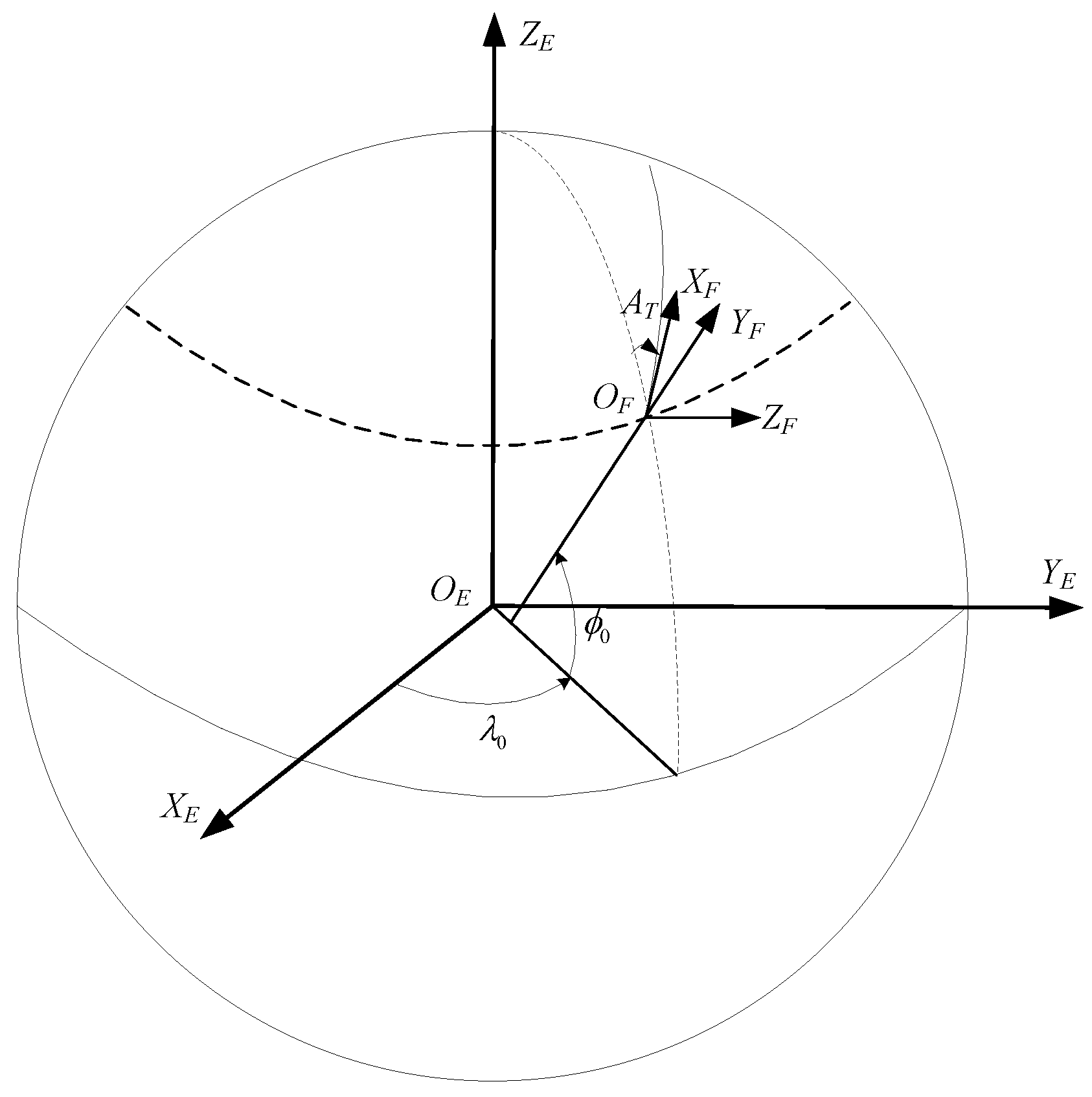
To describe the positions and the law of motion of the flight vehicle, the Earth-Centered–Earth-Fixed (ECEF) system and the Launch Coordinate system (LCS) are commonly employed. The sample data involved in this paper are generated in the LCS. Therefore, the LCS is used as the reference system to explore how the rocket-powered trajectory calculation characteristic parameters are determined.

As shown in Figure 2, the $X_E{Y}_E{Z}_E$ coordinate system is the ECEF system and the $X_F{Y}_F{Z}_F$ coordinate system is the LCS. The starting point of the flight vehicle is $O_F$, the $O_F{Y}_F$ axis is defined by a vertical line through the starting point, the upward direction is positive, and the $O_F{X}_F$ axis is perpendicular to the $O_F{Y}_F$ axis and points in the direction of aiming. At the starting point, the angle $A_T$ between the $O_F{X}_F$ axis and due north along the astronomical meridian is referred to as the geodetic azimuth of the starting point. The $O_F{Z}_F$ axis together with the $O_F{X}_F$, $O_F{Y}_F$ axis forms a right-handed right-angle coordinate system. After the longitude, latitude, and altitude of the starting point and the target point are determined, the geodetic azimuth can be calculated through inverse geodetic algorithm. Then, the position of the LCS is completely determined, and thus a standard rocket-powered trajectory curve is determined.

In order to acquire a large volume of samples, the rocket-powered trajectory calculation characteristic parameters need to be gridded at specific intervals and arranged in combinations to form multiple sets of initial parameters. To ensure broad sample coverage and persuasive representation, it is necessary to determine the scopes for each characteristic parameter prior to the gridding. Assuming the latitude, longitude, and altitude of the starting point and target point as characteristic parameters, the scope of the latitude and longitude of the target point cannot be precisely determined. Therefore, based on the principles of geodetic direct and inverse calculation, this study utilizes the latitude, longitude, altitude of the starting point, the range, the geodesic azimuth, and the altitude of the target point as characteristic parameters. Furthermore, considering the Earth as a homogeneous rotating ellipsoid and assuming the same flight environment corresponding to each rocket-powered trajectory, the variation in longitude at the starting point has minimal influence on the flight trajectory. That is, after other characteristic parameters are determined, the standard trajectory remains consistent at each longitude. Consequently, the longitude of the starting point is removed and the latitude, altitude of the starting point, the range, the geodesic azimuth, and the altitude of the target point are chosen as the final characteristic parameters. For ease of description, the relevant parameter symbols are defined as shown in

Table 1. Definition of relevant parameter symbols.

Symbol	Definition
lat_s	latitude of starting point
lon_s	longitude of starting point
alt_s	altitude of starting point
lat_t	latitude of target point
lon_t	longitude of target point
alt_t	altitude of target point
R	range
A	geodetic azimuth
${\mathit{T}}_0$	the first-stage shutdown time
${\mathit{T}}_1$	total flight time
Az	aiming azimuth angle

.

3.2. Training Data Generation

For DNNs, the quality of the sample data sets the upper limit for the predictive performance of model. Hence, training samples should strive to cover all possible scenarios of the problem. After determining the rocket-powered trajectory calculation characteristic parameters, the scopes and intervals for each parameter are further defined. These intervals are established based on a comprehensive assessment of the hardware conditions in the computing platform and the corresponding training effects of different intervals.

Following the ranges and intervals outlined in

Table 2. The scope and interval for characteristic parameters.

Parameter	Scope	Interval
lat_s	8–56°	4°
alt_s	0–5 km	1 km
alt_t	0–5 km	1 km
$\mathit{R}$	200–600 km	20 km
$\mathit{A}$	0–360°	6°

for gridding, a total of 599,508 sets of rocket-powered trajectory initial parameters will be generated. Should all initial parameters prove valid, this would result in 599,508 individual trajectories. Upon determining the position of the starting point, a gridding representation of the range and the Geodetic azimuth angle is depicted in Figure 3.

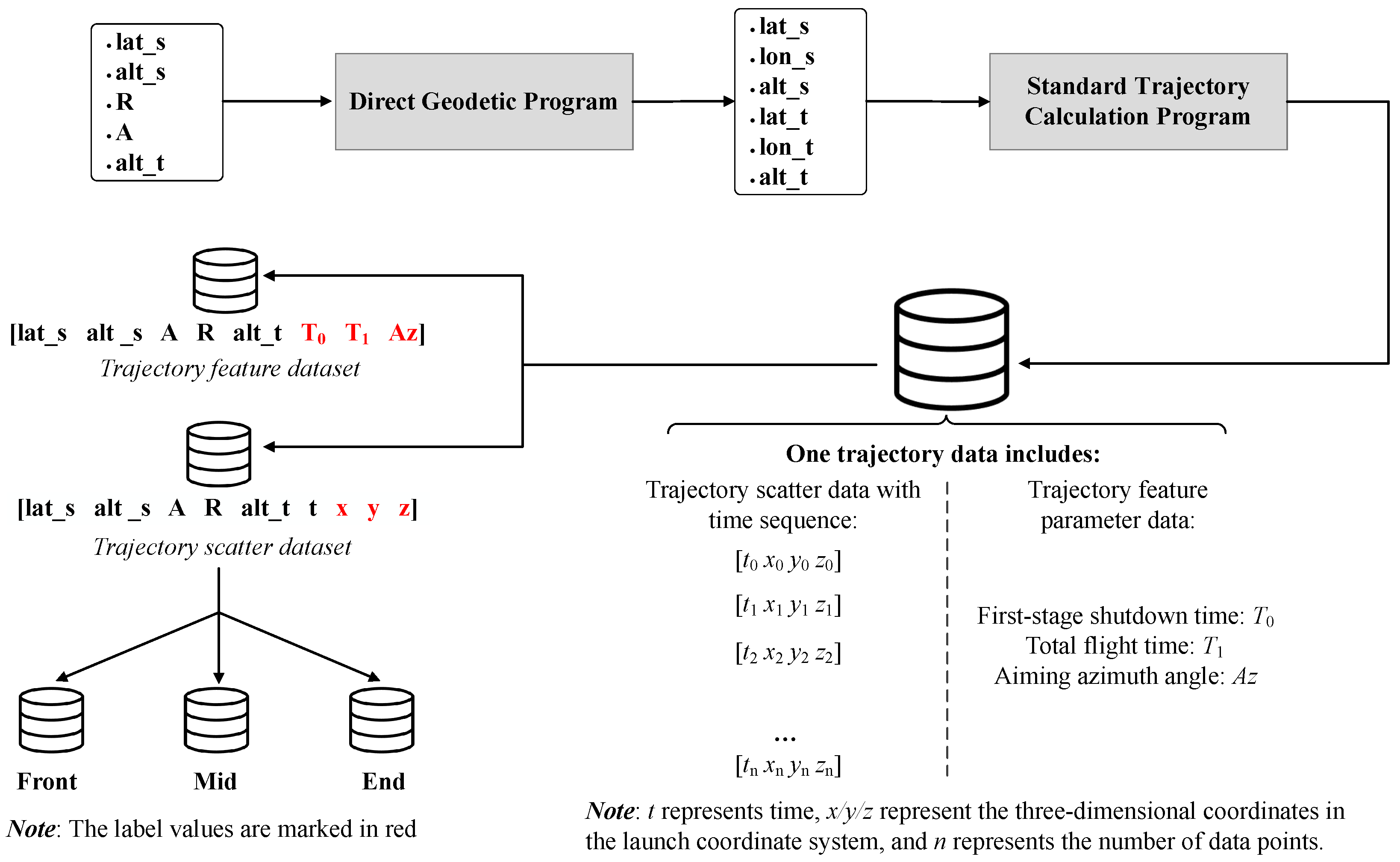
After obtaining multiple sets of initial parameters, the corresponding geographic coordinates of the starting point and the target point are computed by direct geodetic algorithm. Then, the trajectory data is calculated using a standard trajectory calculation program. As for the principles of the standard trajectory calculation program, it involves fourth-order Runge–Kutta numerical integration based on the motion model of a flight vehicle. Its solution process follows the following assumptions: (1) Under the action of the control system, the vehicle is always in an instantaneous torque equilibrium state; (2) The Euler angles involved in the computation are considered to be small quantities, meaning that their sine values are approximated by their radian values, and their cosine values are taken as 1. When products of these angle values appear, they are treated as higher-order terms and thus neglected. Upon acquiring multiple raw trajectory data, further processing is required to derive both trajectory feature data samples and trajectory scatter data samples (processed into three segments: Front, Mid, and End), where the trajectory scatter data unfolds each trajectory in a chronological sequence. The specific workflow for sample generation is illustrated in Figure 4.

3.3. Segmented Training Strategy Based on Domain Knowledge

The segmented training strategy refers to segmenting trajectory scatter data into three segments, as shown in Figure 4, to train the neural networks of different structures and obtain corresponding models. The segmented training strategy is designed based on the domain-specific knowledge regarding the dynamics and segmented aerodynamic effects of a rocket-powered vehicle. According to whether the main engine of the flight vehicle is working or not, the flight trajectory is divided into active and passive segments. Furthermore, based on the extent of aerodynamic forces acting on the vehicle, the passive segment can be divided into the free-flight segment and the re-entry segment. Thus, the flight process of the vehicle is sequentially divided into an active segment, a free segment, and a re-entry segment.

In the active segment, the main forces acting on the flight vehicle include gravity, engine thrust, aerodynamic forces, control forces, and the corresponding moments they generate. During the free-flight segment, the influence of gravity on the flight vehicle is significantly greater than that of aerodynamic forces. In contrast, the braking effect of the aerodynamic force on the flight vehicle is much greater than the influence of gravity in the re-entry segment, resulting in intense aerodynamic heating that is markedly distinct from those in the free-flight phase. Overall, the force conditions experienced by the vehicle vary significantly across the different flight phases, resulting in distinct differential equations of motion for each segment. Therefore, during model training, neural networks with different structures are required to fit the nonlinear relationships corresponding to the equations of motion in each phase, thereby improving the overall prediction accuracy of the trained model. In conclusion, the segmented training strategy is theoretically supported and enhances the interpretability of the multi-scaled neural networks model.

For the trajectory scatter data, segmentation boundaries are defined as follows: each trajectory scatter data from time 0 up to the first-stage shutdown time $T_0$ is divided into the Front sample (for the active segment). Given that the free-flight segment typically constitutes 80% to 90% of the total trajectory time and the maximum flight time in the samples is 666.1 s, it can be concluded that the combined duration of the re-entry and active segment totals approximately 133 s at most. Using the first-stage shutdown time as the endpoint of the active segment, it is observed that the minimum shutdown time among all samples is 58.6 s, implying that the maximum duration of the re-entry phase in the samples is approximately 74.4 s. Given a time interval of 1 s between scatter data points, the last 80 rows of scatter data for each trajectory are selected as the End sample (for the re-entry segment), while the remaining intermediate scattered data is assigned as the Mid sample (for the free-flight segment).

4. DNN Optimization

The trajectory scatter data samples—Front, Mid, and End—along with the feature data samples are used to train Model_Front, Model_Mid, Model_End, and Model_Feature, respectively. Among them, the input and output of Model_Front, Model_Mid, and Model_End are identical and collectively defined as $X_{\mathrm{input}}=\{lat\_s,alt\_s,A,R,alt\_t,t\}$, $X_{\mathrm{output}}=\left\{x,y,z\right\}$. Meanwhile, the input and output of Model_Feature are defined as $X_{\mathrm{input}}=\{lat\_s,alt\_s,A,R,alt\_t\}$, $X_{\mathrm{output}}=\{{\mathit{T}}_0,{\mathit{T}}_1,Az\}$. Once the inputs and outputs of neural networks are determined, additional relevant hyper-parameters for training DNN need to be defined. The primary parameters involved in the process of training are listed in

Table 3. Definition of the main training parameters.

Parameter	Definition
num_layers	number of hidden layers
num_units	number of hidden layer neurons
active_func	activation function, the common ones are ReLU, LeakyReLU, sigmoid and tanh
batch_size	the number of samples selected for a training session
epochs	number of iterations for a batch
lr	learning rate
optimizer	directs the loss function to approach the global minimum in the process of backpropagation, common optimizers are SGD and Adam
lr_change	forms of dynamic decline in learning rate, the commons ones are step, step_warmup and cosine_warmup
n	the downsampling interval of training data, one data is sampled for every other data

.

The approach for determining the structure and training parameters of Model_Front, Model_Mid, Model_End, and Model_Feature is essentially the same. Thus, the subsequent optimization process will be elucidated using the training of Model_Front as an illustrative example.

4.1. Feature Normalization

After determining the sample features and labels, normalizing the data is crucial to eliminate the influence of the base unit and value ranges among the features. In this work, a Min-Max normalization technique is employed, linearly transforming the raw data columns to fall within the [0, 1] range. The normalization formula is expressed as

$$X_{\mathrm{norm}}={\displaystyle \frac{X-X_{\min }}{X_{\max }-X_{\min }}}$$

(6)

where X is the original data, $X_{\mathrm{norm}}$ is the normalized data, $X_{\max }$ is the minimum value of each feature, and $X_{\min }$ is the maximum value of each feature.

4.2. Loss Function Design

The prediction of trajectories is fundamentally a regression problem, where the Mean Squared Error (MSE) function is commonly utilized as the loss function. However, concerning the trajectory scatter data in the LCS, the z-label data values are relatively smaller compared to the x-label and y-label. As a result, the traditional MSE function tends to diminish the impact of errors associated with the z-label on the weight updates during error backpropagation, leading to suboptimal weight updates. To address this imbalance, a weighting matrix is introduced to amplify the error contribution of z-label values, enabling the better learning of z-label values.

Define the number of rows of data for a batch as m, and the corresponding predicted value matrix is

$$Y=\left[\begin{array}{ccc}{y}_{11}& y_{12}& y_{13}\\ ⋮& ⋮& ⋮\\ y_{m1}& y_{m2}& y_{m3}\end{array}\right]$$

(7)

and the real value matrix is

$$\widehat{Y}=\left[\begin{array}{ccc}{\widehat{y}}_{11}& {\widehat{y}}_{12}& {\widehat{y}}_{13}\\ ⋮& ⋮& ⋮\\ {\widehat{y}}_{m1}& {\widehat{y}}_{m2}& {\widehat{y}}_{m3}\end{array}\right]$$

(8)

then the corresponding variance loss matrix can be obtained by (7) and (8):

$$L=\left[\begin{array}{ccc}{l}_{11}& l_{12}& l_{13}\\ ⋮& ⋮& ⋮\\ l_{m1}& l_{m2}& l_{m3}\end{array}\right]$$

(9)

where $l_{mn}={({\widehat{y}}_{mn}-y_{mn})}^2,m\in [1,m],n\in [1,2,3]$

Define the weight matrix

$$w={\left[\begin{array}{ccc}{w}_1& w_2& w_3\end{array}\right]}^T$$

(10)

where $w_1$, $w_2$, $w_3$ are the error weights corresponding to x-label, y-label, and z-label, respectively. Therefore, the final average loss function is

$$\mathit{loss}={\displaystyle \frac{1}{m}}\mathit{sum}\left(L·w\right)$$

(11)

where $\mathit{sum}\left(\right)$ means to sum the elements of the matrix.

In this way, the learning degree of each label during the error backpropagation process can be adjusted by fine-tuning w.

4.3. Activation Function, Optimizer, and Learning Rate

4.3.1. Selection of Activation Function

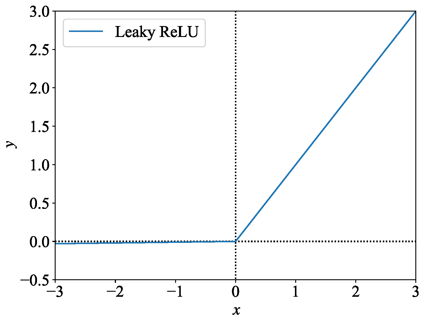
To avoid the problem of neuron death, the LeakyReLU function is chosen as the activation function, as illustrated in Figure 5. The specific expression is

$$\mathrm{LeakyReLU}\left(x\right)=\left\{\begin{array}{cc}x,& \mathrm{if}x\ge 0\\ 0.01x,& \mathrm{otherwise}\end{array}\right.$$

(12)

4.3.2. Selection of Optimizer

Compared to other optimizers (like Stochastic Gradient Descent, SGD), the Adam optimizer performs better when dealing with large datasets [33]. Given the large number of data samples involved in this study, the Adam optimizer is chosen.

4.3.3. Learning Rate (LR)

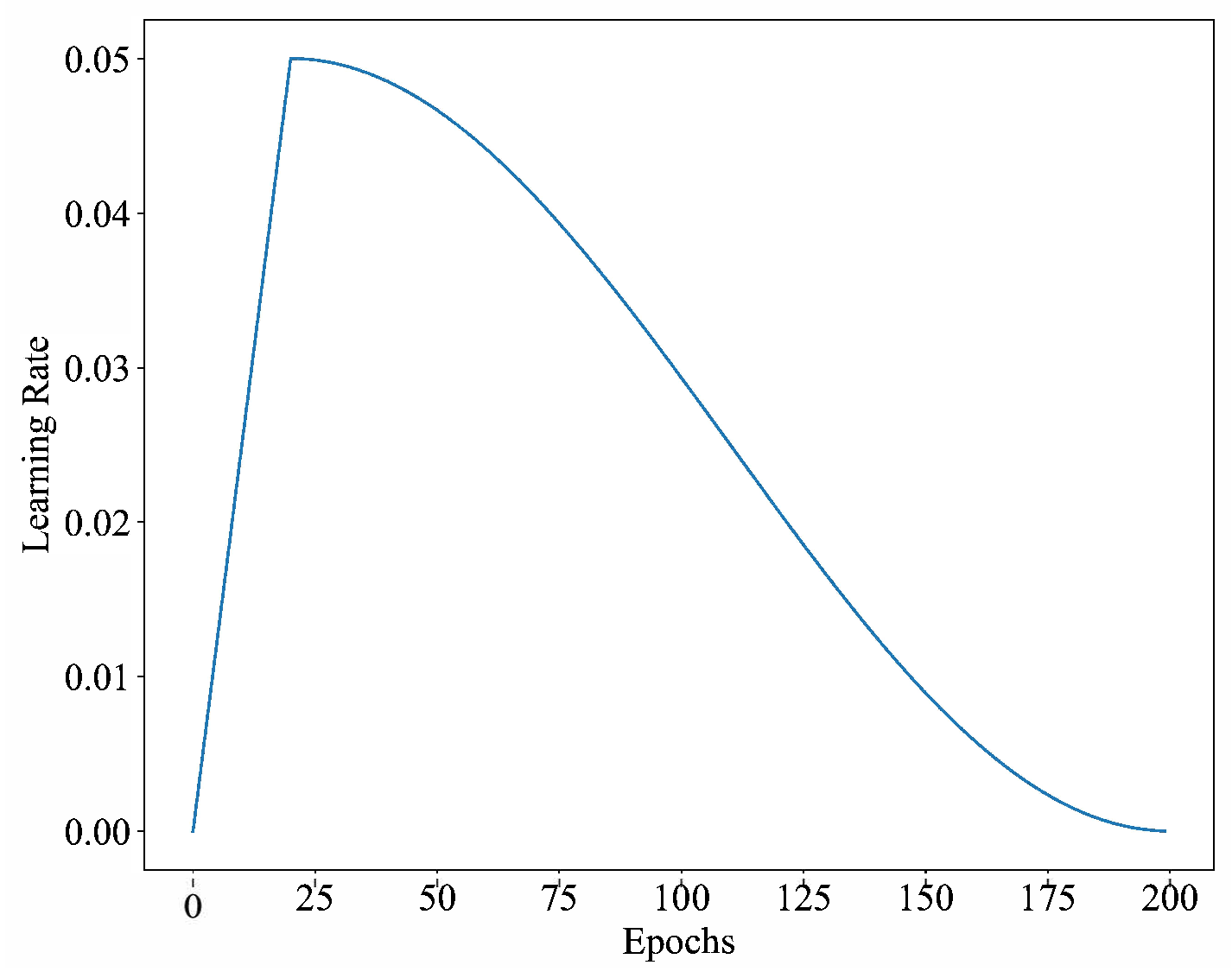
To improve the training efficiency and effectiveness, a dynamically varying learning rate is used, and its changing form is called “cosine_warmup”. At the beginning of training, the learning rate increases linearly to the specified value and then decreases in a cosine fashion.

In Figure 6, the vertical axis of the graph represents the learning rate, and its maximum value is set to 0.05; the horizontal axis represents the epochs, for a total of 200. During the first 1/10th of the epochs, the learning rate increases linearly from 0 to 0.05, and after that, the cosine-decays to 0 from 0.05.

4.4. Determination of Network Structure

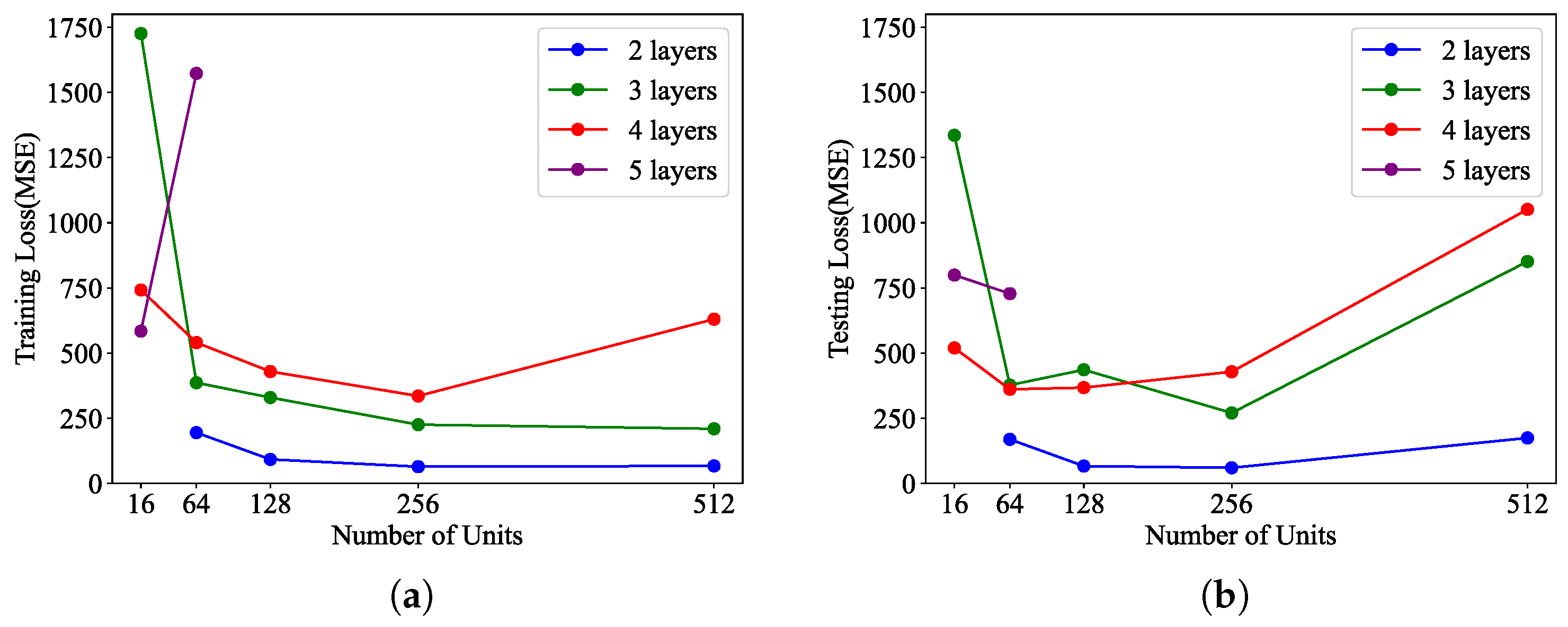
The network architecture is a crucial factor influencing the training effectiveness of neural network, setting the lower limit for the training effectiveness. Changing the number of hidden layers or the number of neurons per layer essentially increases the total number of neurons in the network, enhancing model complexity, and its fitting capability. Too few hidden layers or neurons can result in underfitting, while an excessive number can prolong the training time and potentially lead to overfitting. In this paper, assuming the same number of neurons per layer, the number of hidden layers and the number of neurons per layer are determined by cross-validation.

As illustrated in Figure 7, the training error and testing error corresponding to different combinations of layers and units are recorded and analyzed. The results lead to the following conclusions: first, with a fixed number of units, an increase in layers results in the increase in training and testing errors; second, with a fixed number of layers, an increase in units showcases a trend of decreasing-then-increasing or decreasing-then-stabilizing in training and testing errors. Based on the above analysis, a network structure with 2 hidden layers and 256 units per layer is selected. This architecture achieves low training and testing error, indicating superior learning performance and generalization capability.

4.5. Determination of Learning Rate

The learning rate (LR) is a tuning parameter that affects the convergence speed and learning effectiveness of deep neural networks. To determine a suitable LR that allows the model to achieve optimal loss without compromising training speed, certain training experiments using different LR values on the network structure are defined in Section 4.4 are conducted.

The outcomes are illustrated in Figure 8 and several conclusions can be drawn: a smaller LR can decrease fluctuations in training and validation losses, but an excessively small LR will significantly slow down the convergence speed. Therefore, to strike a balance between accuracy and computational load, a learning rate of 0.001 is selected for subsequent experiments.

4.6. Summary of Training Parameters

Following the above optimization ideas of model training, the optimal architecture and training parameters of all models are finalized as summarized in

Table 4. Main training parameters.

Model	num_layers	num_units	batch_size	epochs	LR	w	n
model_Front	2	256	1024	200	0.001	$[0.3,0.3,0.4]$	1
model_Mid	4	256	1024	200	0.001	$[0.3,0.3,0.4]$	2
model_End	2	256	1024	200	0.001	$[0.3,0.3,0.4]$	1
model_Feature	3	64	64	200	0.0001	$[0.5,0.5]$	0

, where n denotes the number of sampling interval rows in the original samples.

5. Simulation Results

5.1. Multi-DNN Cooperation Strategy

The ranges of t for model_Front, model_Mid, and model_End are determined by the maximum and minimum values of the time features in their corresponding training sets. The specific determination process is as follows: Assuming the ranges of t for front, mid, end datasets are $\left[0,{\mathit{t}}_{\mathrm{front}\_\max }\right]$, $\left[{\mathit{t}}_{\mathrm{mid}\_\min },{\mathit{t}}_{\mathrm{mid}\_\min }\right]$, and $\left[{\mathit{t}}_{\mathrm{end}\_\min },{\mathit{t}}_{\mathrm{end}\_\max }\right]$, respectively. So, in the inference process, the ranges of t for inputs to model_Front, model_Mid, and model_End are, respectively, determined as $[0,\lfloor ({\mathit{t}}_{\mathrm{front}\_\max }+{\mathit{t}}_{\mathrm{mid}\_\min })/2\rfloor ]$, $[\lceil ({\mathit{t}}_{\mathrm{front}\_\max }+{\mathit{t}}_{\mathrm{mid}\_\min })/2\rceil ,\lfloor ({\mathit{t}}_{\mathrm{mid}\_\max }+{\mathit{t}}_{\mathrm{end}\_\min })/2\rfloor ]$, $[\lceil ({\mathit{t}}_{\mathrm{mid}\_\max }+{\mathit{t}}_{\mathrm{end}\_\min })/2\rceil ,{\mathit{T}}_1]$, respectively.

A complete trajectory prediction process is shown in Algorithm 1.

Algorithm 1: Multi-DNN cooperation.

5.2. Analysis of Prediction Accuracy

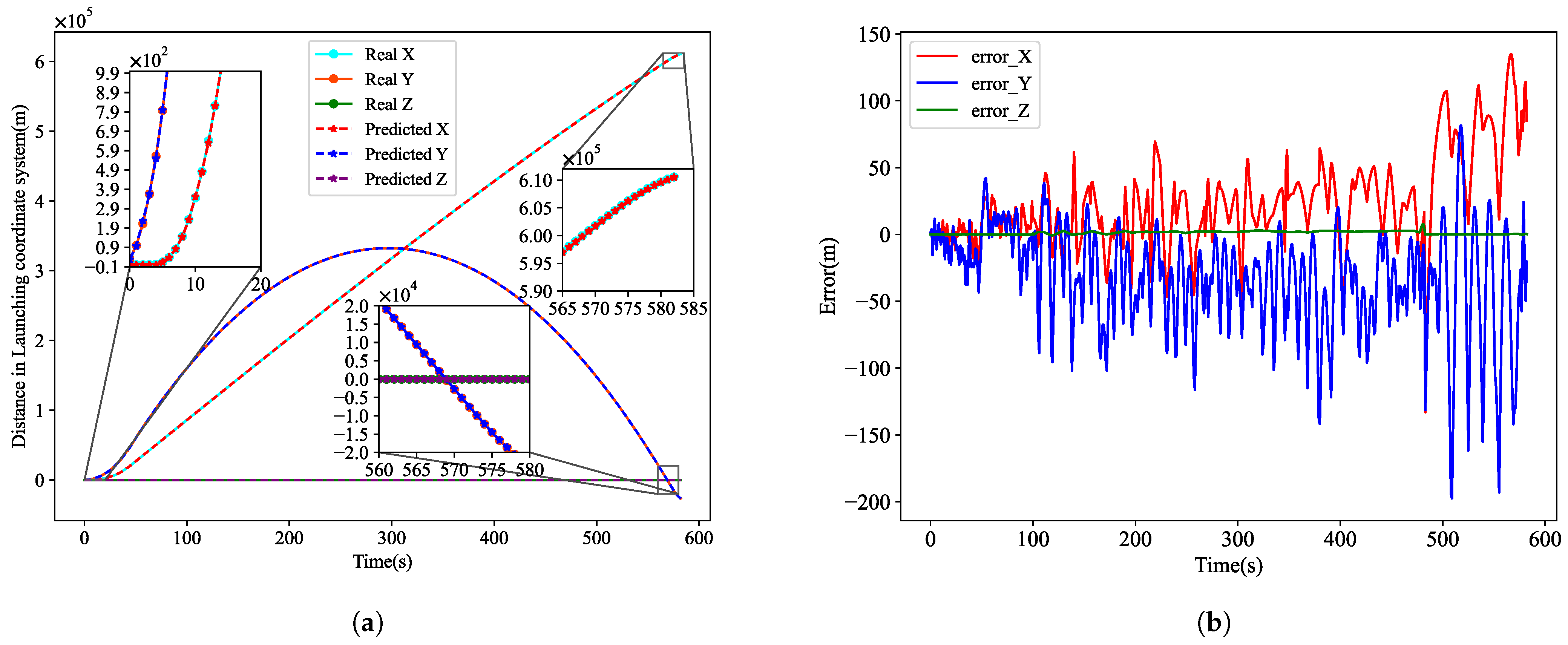
To evaluate the performance of the “trajectory generator” based on multi-scale network fusion, a set of initial parameters [42°,1000,210,611111,4000] (not in the training and testing sets) is randomly selected. The prediction accuracy of the “trajectory generator” is assessed by comparing the trajectory predicted with the trajectory obtained through traditional iterative calculation methods.

Figure 9a illustrates the comparison of the distance at each moment in the x, y, and z directions in the LCS. Notably, the distances in the z direction are mostly around 0. Figure 9b shows the corresponding errors. The errors are analyzed as follows:

(1) The z directional values are primarily close to 0, and are significantly different from those in the x and y directions. Yet, prediction error in the z direction is minimal, so the learning effectiveness in the z direction has not been significantly affected by large difference in the labels, indicating the effectiveness of the loss function designed in Section 4.2.

(2) Errors in the x, y directions tend to increase toward the later stages of the flight. This trend is due to the increasing label values in the x, y directions over flight time. Consequently, the magnitude of the mean squared error becomes considerably larger, resulting in relatively poorer convergence compared to earlier flight stages, finally causing a slight increase in errors.

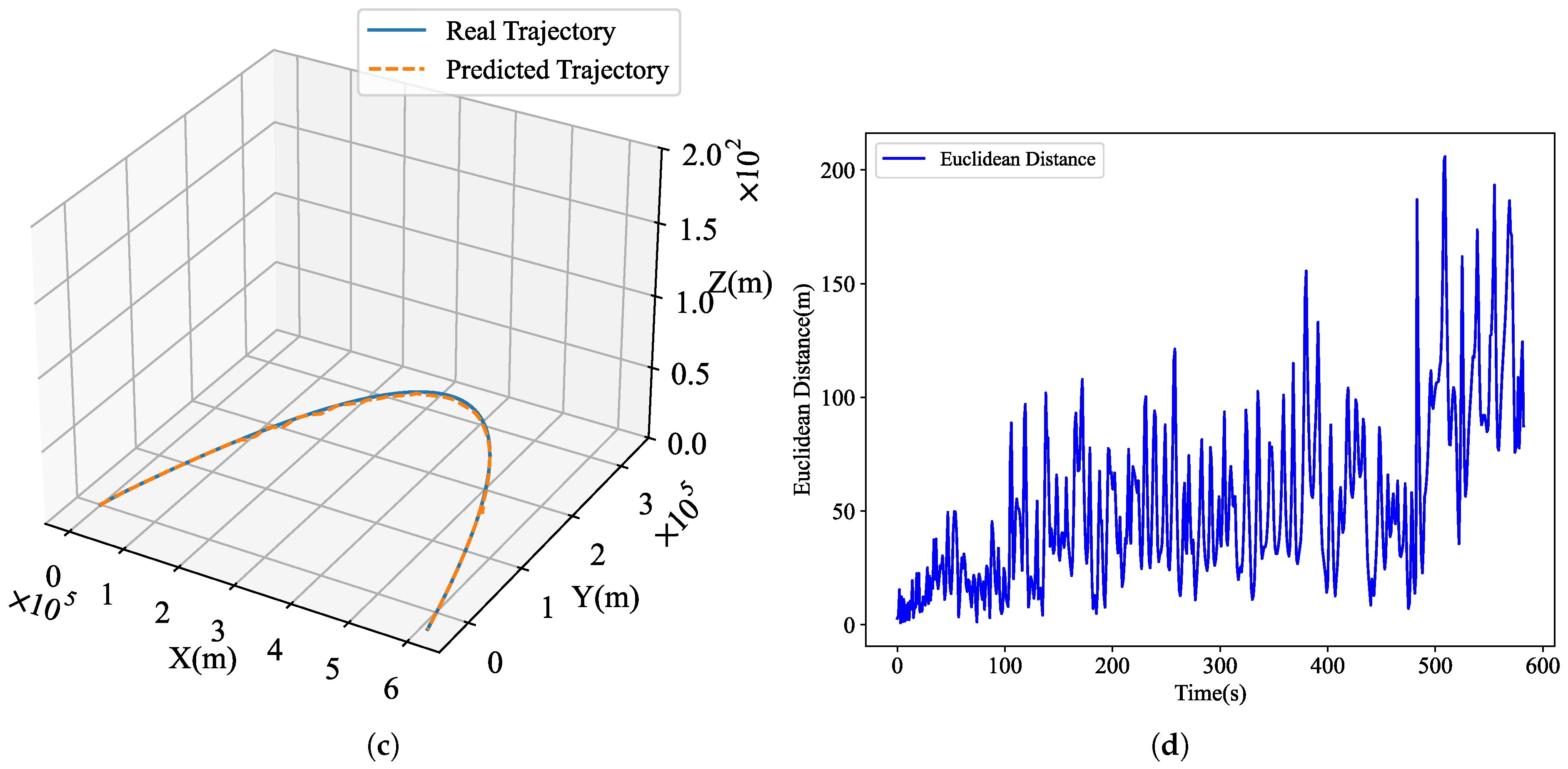
Figure 9c displays a comparison of the complete flight trajectory in the LCS, while Figure 9d illustrates the Euclidean distance between the actual and predicted positions at each moment, representing the prediction error in three-dimensional space. Observing Figure 9d, it is evident that the Euclidean distance slightly increases over flight time, similarly to the marginal increase in errors in the x and the y directions depicted in Figure 9b. Overall, the majority of instances correspond to Euclidean distances below 100, with distances ranging between 100 and 200 in the later stages of flight. Such predictive accuracy is viable for providing trajectory simulation verification for the process of MPDM for multi rocket-powered vehicles.

5.3. Monte Carlo Simulation

To further validate the generalization capability of the models, Monte Carlo simulations and error analyses are conducted. A total of 1320 sets of trajectory calculation parameters are randomly generated. The trajectory data predicted by the DNN-based method is compared with that computed by the traditional iterative calculation method to derive the statistical details of the associated errors.

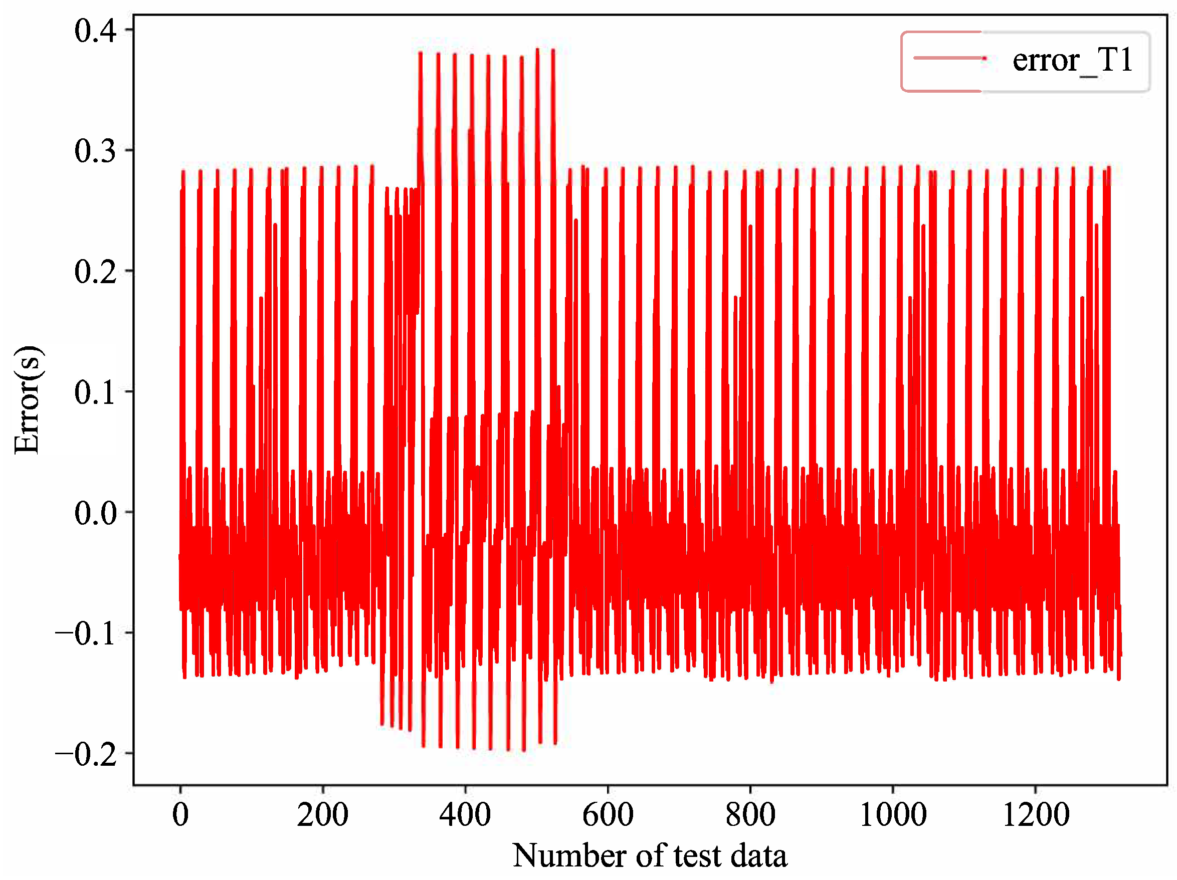
Before comparing the trajectory data, it is important to briefly outline the predictive accuracy of model_Feature, as the algorithm 1 relies on its prediction of T₁. Figure 10 illustrates the T₁ prediction error curve for the 1320 test cases, with a maximum error not exceeding 0.33 s. This error margin satisfies the accuracy requirements for the overall trajectory prediction.

Next, the maximum value, minimum value, median value, and average value of the absolute error corresponding to each trajectory are statistically analyzed, and the following box chart is obtained as shown in Figure 11.

Based on the box plot of maximum values, it is evident that the maximum error in the x, y direction for each predicted trajectory is around 200 m. This indicates a good stability in the model predictions, without any significantly anomalous results. Simultaneously, within the median box plot, the median error in the x, y direction mostly lies around 20 m. This signifies a high level of prediction accuracy for the majority of the time sequence data, as also evident from the box plot of the mean values. The specific maximum, minimum, median, and mean values of errors are as

Table 5. Specific errors of the Monte Carlo simulation.

Error	Max	Min	Median	Mean
X (m)	198.7625	0.0	20.2602	25.4981
Y (m)	217.7961	0.0	21.3373	29.0140
Z (m)	8.6060	0.0	1.2806	1.1997

.

5.4. Validation of Segmentation Strategy

The main innovation of this paper lies in utilizing a segmentation training strategy to enhance the prediction accuracy. To demonstrate the feasibility and effectiveness of this strategy, models trained without a segmentation strategy are used for prediction on the same Monte Carlo simulation data in Section 5.3, obtaining statistical information on the corresponding prediction errors. The network structure and training parameters employed in the non-segmented training are illustrated in

Table 6. Main training-related parameters.

Model	num_layers	num_units	batch_size	epochs	LR	w	n
No segmen_tation model	4	256	1024	200	0.001	$[0.3,0.3,0.4]$	2

.

To better highlight the effectiveness of the segmented training strategy,

Table 7. Comparison of prediction errors between segmented and unsegmented training.

Error (m)	X				Y				Z
	Max	Min	Median	Mean	Max	Min	Median	Mean	Max	Min	Median	Mean
model with segmentation	198.76	0.00	20.26	25.50	217.80	0.00	21.34	29.01	8.61	0.00	1.28	1.20
model without segmentation	1142.82	0.00	293.40	361.32	2525.80	0.00	393.53	667.39	30.66	0.00	0.36	0.61

shows the prediction errors of the DNN models corresponding to the segmented and non-segmented training strategies under the same Monte Carlo experiments.

Frome Table 7, one can see that it is evident that the maximum and average prediction errors of the models trained without segmentation are approximately ten times higher than those trained with segmentation strategy. It demonstrates that the segmentation training strategy is effective in reducing the overall prediction errors and enhancing prediction stability.

5.5. Analysis of Calculation Time

The aim of this study is to achieve the rapid prediction of rocket-powered trajectory at the millisecond level while ensuring accuracy, meeting the real-time requirements of mission planning and decision-making. The number of computational parameters and multiply-accumulate operations (MACs) of the trajectory generator are counted, with the results being 345.548 K and 0.34779 M, respectively. An actual inference time testing program was run to measure the solving time of the “trajectory generator” when predicting different numbers of trajectories. Meanwhile, to make a comparison, the solving time of the traditional iterative calculation method was also recorded. The traditional method was primarily executed on an Intel(R) Core(TM) i7-10700 CPU, while the inference time of the DNN-based method was tested on an NVIDIA GeForce GTX 1050 Ti GPU.

According to the results in the above

Table 8. Statistics of rocket-powered trajectory solution time.

Method	One Trajectory	Five Hundred Trajectories	A Thousand Trajectories
Traditional iterative calculation method	1.585 s	811.285 s	1703.376 s
Trajectory generator	0.019 s	0.176 s	0.321 s

, the DNN-based method can realize a millisecond-level trajectory solution. Particularly when considering the solving time for 1000 rocket-powered trajectories, the DNN-based method has a significant advantage in large-scale rocket-powered trajectory calculations and can meet the real-time requirement of MPDM for rocket-powered vehicle swarm.

6. Conclusions

This paper introduced a DNN-based method for predicting the trajectory of a rocket-powered vehicle, which achieves millisecond-level rapid trajectory prediction while ensuring prediction accuracy, thus meeting the real-time requirements of mission planning and decision-making for rocket-powered vehicles. The final trajectory generator is obtained through the fusion of multi-DNN models, which were developed using a segmented training strategy based on the characteristics of actual trajectory segments. The trajectory generator can predict any single trajectory launched within the national territory in milliseconds while maintaining a prediction error at the scale of 100 m. Moreover, it can simultaneously predict 1000 full trajectories in just 321 milliseconds, showcasing excellent scalability and computational efficiency. Simulation results verify the effectiveness of the segmented training strategy, while comprehensive analysis further confirms the proposed method’s strengths in prediction accuracy, generalization ability, stability, and runtime performance.

The method proposed in this paper is applicable to trajectory prediction for various types of aircraft; however, when formulating segmented strategy, it is essential to consider the specific trajectory characteristics of each type of aircraft. Additionally, in future work, distributed model inference methods can be employed to further reduce the time required for trajectory generation in large-scale scenarios.