Abstract
For the airfoil in freestream, the pressure difference between the upper and lower surfaces and the variations in pressure gradients are significant at its leading edge area. Under reasonable deflections, the active leading edge can effectively change airfoil aerodynamic loads, which helps to improve the rotor aerodynamic performance. In this paper, a modeling method for an airfoil with an active leading edge was developed to calculate its aerodynamic loads. The pitch motion of the rotor blade and the leading edge deflections were taken into account. Firstly, simulations of steady and unsteady flow for the airfoil with an active leading edge were conducted under different boundary conditions and with different leading edge deflection movement. Secondly, the rational function approximation (RFA) was employed to establish the relationship between aerodynamic loads and airfoil/active leading edge deflections. Then, coefficient matrices of the RFA approach were identified based on a limited number of high-fidelity computational fluid dynamics (CFD) results. Finally, an aerodynamic model of the airfoil with an active leading edge was developed, and its accuracy was validated by comparing it to the high-fidelity CFD results. Comparative results reveal that the developed model can calculate the aerodynamic loads of an airfoil with an active leading edge accurately and efficiently when applied appropriately. The modeling method can be used in aerodynamic load calculations and the aeroelastic coupling analysis of a rotor with active control devices.
1. Introduction
Vibration reduction has remained one of the principal challenges in helicopter design and operation for decades. A helicopter rotor is exposed to a large variation in flow, which results from highly unsteady aerodynamic phenomena, including dynamic stall and reversed flow on the retreating side, transonic flow on the advancing side, and blade/vortex interaction (BVI) in certain flight conditions. As a consequence, rotor performance is restricted, and there are severe vibrations [1] in helicopters. Excessive vibrations not only degrade the reliability of airframe structures and onboard equipment, but also affect passenger comfort. Therefore, it is essential to reduce vibrations in helicopters. An active rotor with active control devices, is an effective technology to reduce the vibrations and improve rotor performance. Dynamic deflection of the active control devices enables direct control of the airfoil camber and manipulates its aerodynamics, which is classified as a direct effect [2]. In addition to this, another moment, arising from the active control devices, will affect the torsional deflection and local angle of attack (AoA) of the blade sections. This will, in turn, affect the aeroelastic response of the rotor blades, which is classified as an indirect effect or servo effect. Ultimately, the aerodynamic loads on the rotor and the aeroelastic response of the blades will be influenced, and the undesirable loads and noises can be suppressed at the source. Additionally, active control devices are independent from the primary flight control system, which means there is no safety issue during the flight in the accidental failure of the active control devices. Thus, the active rotor is promising for helicopters in vibration and noise control.
Active control devices can be classified into the active leading edge and the trailing edge flap (TEF), according to their mounting position. Numerous studies on TEF have been completed, and the control authority of TEF on vibrations and noises [3,4,5,6,7,8] has been demonstrated. In comparison, deflections of the active leading edge not only reduce the compressibility effect near the leading edge at high Mach number, but also help to reduce the suction pressure peak and adverse pressure gradients, thus delaying the leading edge separation and stall [9]. The control authority of the active leading edge on the airfoil dynamic stall has been validated. Wind tunnel tests and CFD simulations of VDLE (Variable Droop Leading Edge) were conducted for the VR-12 airfoil [10]. It is observed in this study that the negative torsional damping caused by dynamic stall can be completely eliminated by the variable droop leading edge concept. Similarly, wind tunnel tests of VDLE [11,12] on a full-sized chord blade section indicated that the phase angle variation between blade motion and VDLE contributes to the reduction of drag and moment peaks without lift loss. Niu et al. [13] investigated the airfoil dynamic stall by applying two VDLE motion modes. Their investigations show that the local angle of attack near the leading edge dynamically decreases with the VDLE when the overall angle of attack becomes too large, and in the specific VDLE motion mode, the variation of the airfoil pitching moment is negatively associated with the variation of the angle of attack, which will induce positive damping that can eliminate the instability in pitch oscillation. For the rotor with an active leading edge, aerodynamic loads on the disk can be regulated effectively by actuating the leading edge, and this can help to reduce vibrations and enhance the performance of the rotor simultaneously.
The calculation of aerodynamic loads is important in the studies of rotor with active control devices. To obtain high-fidelity aerodynamic loads, CFD methods have been indispensable due to their accuracy in modeling complex aerodynamic environments. Mishra [14,15] handled the multi-element intermesh connectivity with the implicit hole cutting overset implementation and developed a coupled CFD and CSD (computational structural dynamics) methodology to analyze the effects of a leading edge slat on the rotor performance. This reveals that dynamic deflections of the leading edge slat not only enhance the rotor thrust, but also achieve a reduction of torsional structural loads and pitch link loads as compared to the baseline C9017 values. Similarly, the unsteady flow over the multi-element airfoil [16] was investigated using the CFD method. In this research, the lift coefficient increased by 52.99% with the application of a leading edge slat, and the flow separation at high AoAs was delayed effectively. Under reasonable boundary conditions, the CFD method allows both visualizations of unsteady flow and high-fidelity simulations over the multi-element airfoil in flow field. However, due to the extensive computational durations and suboptimal efficiency, the CFD method is only suitable for high-fidelity simulations in complex flow fields or mission-specific scenarios requiring detailed vortex dynamics resolution.
Currently, aeroelastic coupling analysis is mainly based on the rotating beam model and the 2D sectional aerodynamic model, such as CAMRAD II [17] and RCAS [18]. In calculating aerodynamic loads of the active rotor, there are three types of 2D aerodynamic models, the unsteady Leishman–Hariharan model, the quasi-steady Theodorsen theory, and the table-lookup method based on wind tunnel test data or numerical simulation results. Table-lookup method incorporates steady characteristics of airfoil. However, it is difficult to analyze unsteady effects arising from the airfoil pitch oscillation. In contrast, the Theodorsen theory [19] and Leishman–Hariharan model [20] can capture aerodynamic characteristics of an oscillatory airfoil with active control devices, while they neglect the influence of airfoil geometry on aerodynamics. To study the effectiveness of active control devices, it is essential to develop an unsteady aerodynamic model that takes into account the geometries of the active leading edge, and at the same time, this model should balance computational efficiency with fidelity in capturing vortex-dominated flow, which are important for aeroelastic coupling analysis of the rotor with an active leading edge.
CFD with an overlapping grid approach enables the consideration of geometries of the active leading edge, and captures unsteady aerodynamics in airfoil pitch oscillation. The RFA approach allows for a compact mathematical formulation and exceptional computational efficiency. The aerodynamic model, combining the CFD method and RFA approach, can achieve computational efficiency in aerodynamics, and the accuracy requirement for aeroelastic analysis. This modeling method has been successfully implemented in the aeroelastic analysis of the active rotor with TEFs. A 2D, unsteady aerodynamic model [21] for an airfoil/flap combination and a time-varying compressible freestream was established using the previous methodology. The theoretical analysis of the vibration reduction was also performed for an active rotor with TEFs. Similarly, an unsteady reduced-order model (ROM) [22,23] for the airfoil with TEF was developed based on CFD and RFA, and there is a large improvement in accuracy for calculating unsteady aerodynamic loads when compared to the original RFA model. Investigations of various TEF configurations [24] for vibration reduction were conducted by Padthe, in which CFD results were employed and the relationship between aerodynamic loads and TEF deflections was established in state–space equations. Although the modeling method has been applied in the active rotor with TEFs, there are few studies using this method in aerodynamic loads for the active rotor with an active leading edge.
In this paper, the aerodynamics of an airfoil (NACA0012) with an active leading edge were investigated, considering the gap between the main airfoil and the leading edge. The nonlinear relationship between aerodynamic loads and airfoil/leading edge deflections was established by combining high-fidelity CFD results and a concise RFA approach. The modeling methodology for the airfoil with an active leading edge was validated, which can be employed to analyze the aeroelastic coupling analysis of the active rotor.
2. Methods
In this section, the modeling method for the airfoil with an active leading edge is developed. The complex movements of the airfoil, including plunging, pitching, and motions of the active leading edge, are all taken into account. The CFD method and the RFA approach are employed to develop the aerodynamic model, in which the narrow gap between the main airfoil and active leading edge is considered. The identification process of coefficient matrices in the developed model is described as well.
2.1. Computational Fluid Dynamics (CFD)
For the flow involving relative motions, the overlapping grid approach provides a straightforward way to generate grids, particularly for the unsteady flow within narrow gaps between different components. In simulations, the overlapping grid approach will firstly divide the flow field into several subdomains and generate sub-grids independently for each subdomain. Then, motions of sub-grids are defined, respectively. Additionally, this approach can recognize the interface between the sub-grids and transmit the information required for simulations. Eventually, complicated motions of the system can be transformed into the relative motions between sub-grids.
In the CFD simulations performed in this study, a compressible unsteady Reynolds-averaged Navier–Stokes CFD solver was employed, as shown in Equation (1).
where is the conserved variables, and , are the inviscid flux and viscous flux, respectively. The finite volume method (FVM) was used to solve the Equation (1). A second-order upwind was set for momentum and turbulence. The PRESTO! (PREssure STaggering Option) scheme was used for pressure interpolation, and the method based on least-squares cell was chosen for the gradient. In each of the sub-grids, the flow field will be artificially divided into a certain number of adjacent cells with an arbitrary shape. Therefore, the integral surface in Equation (1) can be expressed, approximately, as the sum of fluxes on each face of the cell. For the cell , the spatial discretization of Equation (1) gives the following form, using the conservation law:
where is the area of cell (the volume in 3D cases), is the length (or area) of the jth edge (or face) of the cell , and is the number of the edge (or face) of the cell . The discretization of subdomains is accomplished by calculating the flux sum over all cells in the region. Consequently, the movements of subdomain grids are defined independently. By then, the combination of the individual motion of the subregional grid characterizes the multi-movements of system. The first-order implicit transient formulation was employed in temporal discretization schemes, and the SST model was chosen to formulate the turbulence over the airfoil with an active leading edge, which can predict flow separation accurately.
The classic overlapping grid approach with direct hole cutting was employed in this study. Faces of cut zones were identified as different types and overlapping cut faces were marked based on adjacent cell sizes and local feature angles. Donor cells were selected based on grid priorities. Cells on overlapping cut faces with the highest grid priority were principal donor cells. These cells, along with those connected by faces or nodes, are used as donor candidates. The linear interpolation algorithm was also utilized to deliver the flow field information through the overlapping boundaries of the sub-grids during the simulation. The linear interpolation was formulated as follows:
where is the cartesian coordinate of the center point for cell . To obtain a detailed description of Equation (3), information about the four background cells adjacent to cell I, denoted as , , , , was required. In that case, the factors in Equation (3) are given by
In simulations, the value of the overlapping grids in the field will be redefined without regeneration of all sub-grids, which thereby significantly simplifies the simulation workflows. For multi-element airfoils, the common meshing method is faced with challenges in precise definition of relative motions and high-fidelity simulations of unsteady flow in narrow gaps. In contrast, the overlapping grid approach is more suitable for this situation.
2.2. Rational Function Approximation (RFA)
During rotation, the motion of blade section mainly originates from the flapping motion and cyclic pitch controls. For the airfoil with an active leading edge, the airfoil motions include plunging displacement z (the blade flapping motion), pitch deflections (pitch controls), and motions of the active leading edge (deflections or displacement of the component).
Given that the translational motion of the small amplitude can be expressed as deflections with its center of deflection located at infinity, motions of the active leading edge can be represented as an independent deflection , which facilitates consistency with the pitch deflections in the expression. Therefore, the generalized motion vector for the airfoil with an active leading edge is expressed as follows:
Lift coefficient , drag coefficient , moment coefficient of main airfoil , and moment coefficient of active leading edge are included in the generalized aerodynamic load vector , which is expressed as follows:
The RFA approach establishes a relationship between generalized aerodynamic loads and generalized motions in the Laplace domain, as follows:
where and represent Laplace transforms of the generalized aerodynamic load vectors and generalized motion vectors, respectively. The aerodynamic transfer matrix [25] is approximated using the least-squares approach with a rational expression of the form shown below.
Equation (8) is usually called the Rogers approximation [26]. The term in the summation is the aerodynamic lag term associated with a number of poles . These poles are assumed to be positive to produce stable open loop roots, but are otherwise non-critical to the approximation.
The Laplace transform representation in Equation (7) is related to the generalized motions and generalized loads, through the following expressions:
where is the time-dependent freestream velocity. Here, the reduced time is used such that unsteady freestream effects can be properly accounted for [21], and can be interpreted as the distance measured in semi-chords. To simplify the derivation of the state space model, the lag terms in Equation (8) are rewritten in matrix form [25] as follows:
where the matrices , , and are given by
and the Equation (8) is rewritten in matrix form as follows:
The rational approximant in Equation (11) can be transformed to the time domain using the inverse Laplace transform, which yields the final form of the state–space model, given in Equations (12) and (13).
where the matrices , and have been given previously. To accurately capture the aerodynamic characteristics, it is necessary to first carry out CFD simulations. Then, the coefficient matrices in Equations (12) and (13) can be identified from the limited number of CFD results. In order to simplify the identification process of the coefficient matrices, the aerodynamic loads are decomposed as follows:
where are the steady components of aerodynamic loads, which correspond to the steady CFD results with far-field freestream (flow velocity and angle of attack ). are the dynamic components of aerodynamic loads, which correspond to the dynamic CFD results with airfoil deflections (). The computational workflow of the developed model is illustrated in Figure 1.
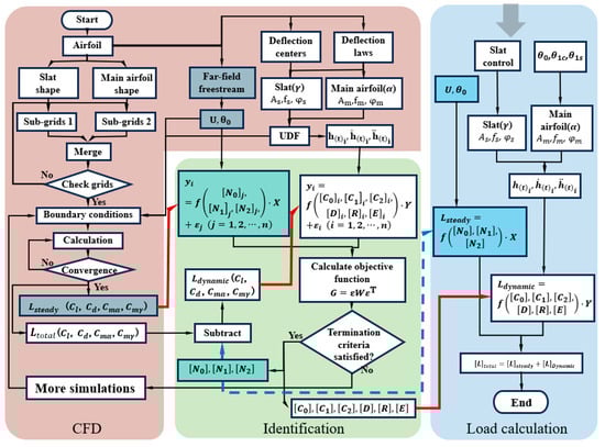
Figure 1.
Aerodynamic loads calculation flowchart of the developed model.
The computational processes of the aerodynamic model, combining the RFA approach and CFD method, are divided into three steps (as shown in Figure 1), as follows:
Step 1. CFD. The steady results and dynamic results will be simulated, respectively, according to shapes of airfoil, flow velocity , angle of attack , and deflections of the airfoil ().
Step 2. Identification. The above and are used in this step. Coefficient matrices and are identified, respectively, with the nonlinear multiple regression model.
Step 3. Load calculation. Under predefined motions, and are calculated, respectively, based on identified coefficient matrices. At last, the total aerodynamic loads can be calculated through the linear superposition of and .
2.3. Identification of Coefficient Matrices
To develop the aerodynamic model for the airfoil with an active leading edge, the steady and dynamic components of aerodynamic loads need to be calculated sequentially. According to the steady components of aerodynamics , the freestream flow velocity , and the angle of attack , the nonlinear multiple regression model [27] is expressed as
where is the multivariate nonlinear function between and the system input. is the vector of system inputs and . are the coefficient matrices that need to be identified. is the jth group of data. is the identification error for the jth group of data.
The objective function in the identification process of a multivariate nonlinear regression model is defined as follows:
where , which represents the steady identification errors for different groups of data. is the weight matrix, through which the weight of each identification error can be properly adjusted. If the identification error reaches its minimum value, the objective function and the identified coefficients should satisfy the following equation:
The coefficient matrices , establishing the relationship between the steady components of aerodynamic loads and the far-field freestream conditions, can be obtained as follows:
For the relationship between the dynamic components of aerodynamic loads and the airfoil deflections (), the nonlinear multiple regression model is expressed as follows:
where is the multivariate nonlinear function between and the system input. is the vector of system inputs . are the coefficient matrices that need to be identified. is the ith group of data. is the identification error for the ith group of data.
The objective function in the identification process of a multivariate nonlinear regression model is defined as follows:
where , which represents the dynamic identification errors for different groups of data. is the weight matrix, as defined before. If the identification error reaches its minimum value, the objective function and the identified coefficients should satisfy the following equation:
The coefficients of the multivariate nonlinear regression model can be obtained as follows:
These coefficients correspond to the matrices , , , , , in the established aerodynamic model.
At this stage, the coefficient matrices and , , , , , establishing, respectively, the relationship between the steady aerodynamic components and freestream conditions, as well as the dynamic aerodynamic components and deflections of airfoil, have been obtained. According to these matrices, the steady and dynamic components of aerodynamic loads for the airfoil with the particular motions are separately calculated.
3. Validations of the Applied Methods
In this section, the effectiveness of the CFD method, based on overlapping grids, and the identification of coefficient matrices of the RFA approach are validated. During the validation, the motion of the active control device and the pitch motions of the airfoil were individually taken into account.
3.1. CFD Method
For the airfoil with active control device, the overlapping grid approach allows for the individual meshing of sub-grids, which are then integrated into the computational grids. This enables aerodynamic simulations of multi-element airfoils undergoing relative motions. To verify the effectiveness of the overlapping grid approach for discontinuous, multi-element airfoils, the multi-element airfoil 30P30N [28,29] was selected. Figure 2 presents the shape of 30P30N, the generated overlapping grids, the pressure distribution on the airfoil surface, and the density contour map in the flow field at the different angles of attack conditions calculated using the overlapping grid approach.
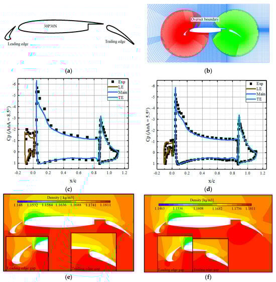
Figure 2.
Validations of the 30P30N multi-element airfoil: (a) the airfoil shape; (b) overlapping grids for simulation (Blue: background grids; red: component grids of leading edge; green: component grids of trailing edge); (c) pressure distribution at AoA = 5.5°; (d) pressure distribution AoA = 8.5°; (e) the flow field density contour map AoA = 5.5°; (f) the flow field density contour map AoA = 8.5°.
As made evident in Figure 2c,d, the pressure distribution on each element of the airfoil was precisely calculated at different AoAs. The simulations show good agreement with the experimental results, which indicates that the overlapping grid approach can be used to simulate the unsteady flow over the airfoil. As can be seen in Figure 2e,f, there is no obvious discontinuity in the density contour map of the flow field, which means the flow field information can be successfully transmitted among the sub-grids for discontinuous, multi-element airfoil.
To validate the fidelity of the overlapping grid approach for dynamic cases, NACA0012 airfoil was used. The parameters are listed in Table 1. The generated overlapping grids and the comparison between CFD results and experimental data are illustrated in Figure 3.

Table 1.
Parameters for validation of dynamic case.
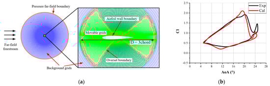
Figure 3.
Validations of NACA0012 airfoil: (a) overlapping grids for calculations (Blue: background grids; green: component grids of airfoil; red: overset boundary grids); (b) comparison between CFD results and experimental data [30].
As seen in Figure 3, for airfoil undergoing dynamic deflections, the overlapping grid approach effectively captures the variation of aerodynamic loads with angles of attack. The simulations demonstrate good agreement with the experimental data.
In summary, the overlapping grid approach applied in this study enables high-fidelity simulations of aerodynamic loads on airfoils. The CFD results demonstrate sufficient accuracy in calculating unsteady aerodynamic loads for multi-element airfoils. The aerodynamic loads from simulations can be used in the identification of coefficient matrices in the developed model.
3.2. Identification Method
Validations of the coefficient matrices from identification were conducted to investigate the effectiveness of the identification method. The aerodynamic loads from coefficient matrices were compared to the high-fidelity CFD results. The grids of the airfoil with an active leading edge and the parameters for simulations are detailed in Table 2 and Figure 4, respectively.
Table 2.
Parameters for simulations.
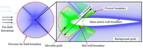
Figure 4.
The grids for CFD simulations (Blue: background grids; green: component grids of active leading edge; red: overset boundary grids).
The effectiveness of active control devices on the rotor results from both direct effects and servo effects; that is, the influence of active control devices on the lift and moment of the airfoil. According to the previous description, aerodynamic loads of the airfoil with an active control device are decomposed into steady and dynamic components. Therefore, validations of the identification method for steady and dynamic cases were carried out sequentially in this section. Simulations of steady and dynamic cases were performed at the Mach number of 0.6.
3.2.1. Steady Components
Coefficient matrices are identified, and they are used to establish the relationship between aerodynamic loads and boundary conditions of the flow field. The objective function in the identification process was defined as follows:
To determine the coefficient matrices , the required parameters for identification are the steady results and angles of attack of the airfoil. Under the same freestream conditions, comparisons are illustrated between the CFD results and the fitted results, derived from the identified coefficient matrices in Figure 5 and Figure 6.
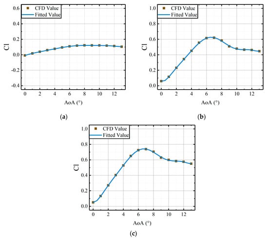
Figure 5.
Comparisons of CFD results and the fitted results, derived from the coefficient matrices, versus AoAs of main airfoil under the steady deflections: (a) the lift coefficients of active leading edge; (b) the lift coefficients of the main airfoil; (c) the lift coefficients of the whole airfoil.
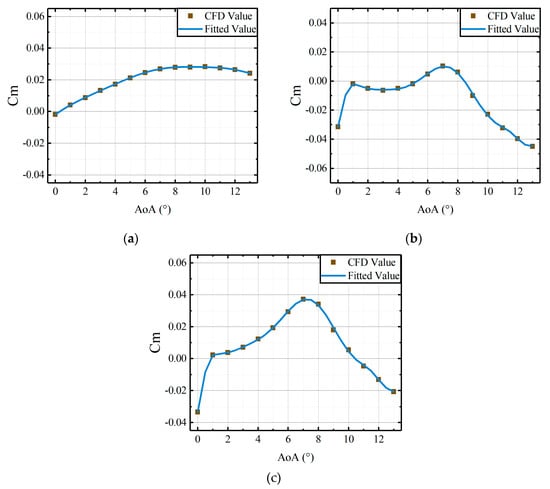
Figure 6.
Comparisons of CFD results and the fitted results, derived from the coefficient matrices, versus AoAs of main airfoil under the steady deflections: (a) the moment coefficients of active leading edge; (b) the moment coefficients of the main airfoil; (c) the moment coefficients of the whole airfoil.
From Figure 5 and Figure 6, it can be observed that the fitted results from identified coefficient matrices are in good agreement with the CFD results. Therefore, the relationship between steady components of aerodynamic loads and the freestream conditions can be established by coefficient matrices. The identification method, based on the nonlinear regression model, can be applied to determine the coefficient matrices of the RFA approach. Within specified freestream conditions (velocity and angle of attack), the coefficient matrices identified from the CFD results can be used to calculate the steady components of aerodynamic loads for the airfoil with an active leading edge.
3.2.2. Dynamic Components
In rotation, the blade pitch motion undergoes cyclic variations, along with the rotor disk. Therefore, the airfoil at the 0.7R position of the blade experiences the cyclic angle of attack variations along with the rotor disk. Moreover, an active leading edge with independent deflections has influences on airfoil aerodynamic loads. In this section, the airfoil with independent leading edge deflections and cyclic pitch motions was investigated. The coefficient matrices, which is used to establish the relationship between dynamic components of aerodynamic loads and airfoil deflections, were identified. The objective function in the identification process is formulated as follows:
where correspond to , , , , and in the coefficient matrices, respectively. The required parameters for identification are the dynamic components of the aerodynamic loads and airfoil deflections . The dynamic components of the aerodynamic loads are calculated by subtracting the steady components, calculated via coefficient matrices , from the dynamic results.
- (1)
- Parameter identification of active leading edge under independent deflections
In this section, the identification of coefficient matrices between the dynamic components of aerodynamic loads and the deflections of the active leading edge was conducted. The deflections of the active leading edge are illustrated in Figure 7.
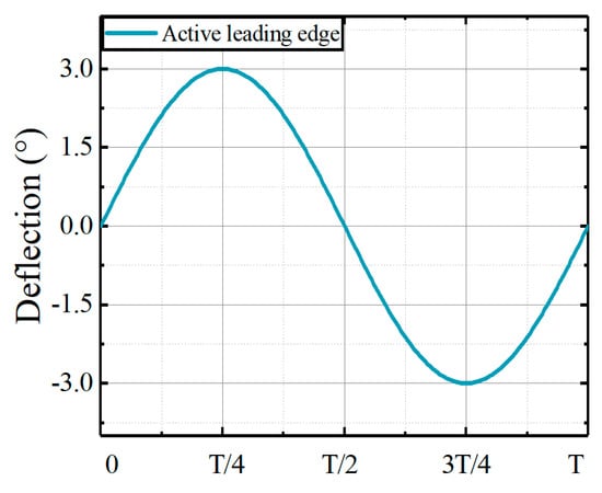
Figure 7.
Deflections of active leading edge.
Investigations were performed at angles of attack of 0°, 2.5°, and 5° to validate the effectiveness of coefficient matrices in calculating aerodynamic loads. The aerodynamic loads calculated from the identified coefficient matrices are compared to CFD results, as shown in Figure 8, Figure 9 and Figure 10.
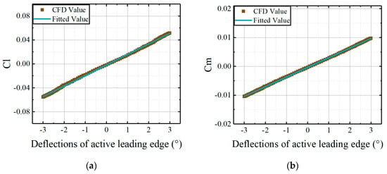
Figure 8.
Comparisons of CFD results and the fitted results, derived from the coefficient matrices, versus deflections of the leading edge at AoA = 0°: (a) lift coefficients of active leading edge; (b) moment coefficients of active leading edge.
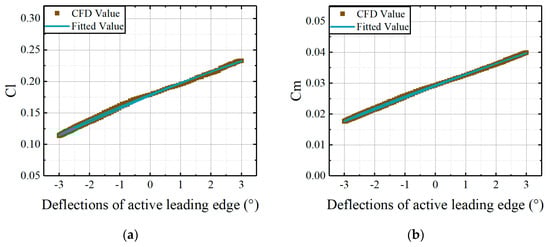
Figure 9.
Comparisons of CFD results and the fitted results, derived from the coefficient matrices, versus deflections of the leading edge at AoA = 2.5°: (a) lift coefficients of active leading edge; (b) moment coefficients of active leading edge.
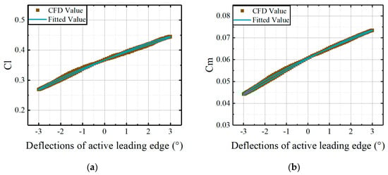
Figure 10.
Comparisons of CFD results and the fitted results, derived from the coefficient matrices, versus deflections of the leading edge at AoA = 5°: (a) lift coefficients of active leading edge; (b) moment coefficients of active leading edge.
As made evident in Figure 8, Figure 9 and Figure 10, the fitted results from the identified coefficient matrices demonstrate good agreement with the CFD results. Therefore, coefficient matrices of the developed model can be determined by the identification method employed in this study. The relationship between aerodynamic loads of the active leading edge and the deflections of that can be established concisely.
- (2)
- Parameter identification of the main airfoil under pitch motions
The dynamic cases employed in this section were simulated, with the active leading edge being stationary to the main airfoil. The pitch motions of the main airfoil are illustrated in Figure 11.
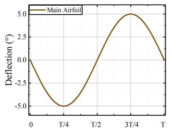
Figure 11.
Deflections of the main airfoil.
Under the deflections of the main airfoil, identifications for the dynamic components of aerodynamic loads on the main airfoil were conducted at angles of attack of 0°, 2.5°, and 5°, respectively. The aerodynamic loads calculated from the identified coefficient matrices are compared to the CFD results, as shown in Figure 12, Figure 13 and Figure 14.
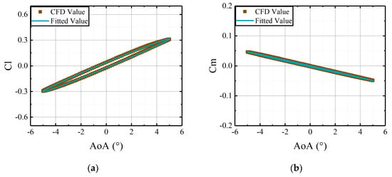
Figure 12.
Comparisons of CFD results and the fitted results, derived from the coefficient matrices, versus deflections of the main airfoil at median AoA = 0°: (a) lift coefficients of main airfoil; (b) moment coefficients of main airfoil.
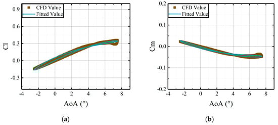
Figure 13.
Comparisons of CFD results and the fitted results, derived from the coefficient matrices, versus deflections of main airfoil at median AoA = 2.5°: (a) lift coefficients of main airfoil; (b) moment coefficients of main airfoil.
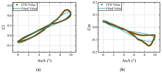
Figure 14.
Comparisons of CFD results and the fitted results, derived from the coefficient matrices, versus deflections of the main airfoil at median AoA = 5°: (a) lift coefficients of main airfoil; (b) moment coefficients of main airfoil.
As made evident in Figure 12, Figure 13 and Figure 14, the variations of aerodynamic loads with deflections of the main airfoil can be described by the coefficient matrices. The fitted results from the matrices are in agreement with the CFD results. Therefore, the identification method applied in this study can determine the coefficient matrices effectively. However, the identification method experiences quantifiable degradation in calculating aerodynamic loads when the stall occurs.
- (3)
- Parameter identification of active leading edge under pitch control
The deflections of the active leading edge originate from the additional actuation. To evaluate the power required for deflections of the active leading edge, it is necessary to identify the coefficient matrices, establishing the relationship between aerodynamic loads of the leading edge and deflections of the main airfoil. The deflections of the main airfoil are illustrated in Figure 11. The fitted results calculated from the identified coefficient matrices are compared to the CFD results, as shown in Figure 15, Figure 16 and Figure 17.
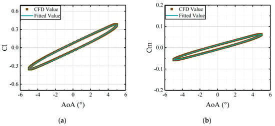
Figure 15.
Comparisons of CFD results and the fitted results, derived from the coefficient matrices, versus deflections of the main airfoil at median AoA = 0°: (a) lift coefficients of active leading edge; (b) moment coefficients of active leading edge.
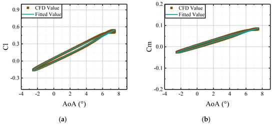
Figure 16.
Comparisons of CFD results and the fitted results, derived from the coefficient matrices, versus deflections of the main airfoil at median AoA = 2.5°: (a) lift coefficients of active leading edge; (b) moment coefficients of active leading edge.
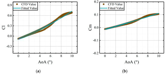
Figure 17.
Comparisons of CFD results and the fitted results, derived from the coefficient matrices, versus deflections of the main airfoil at median AoA = 5°: (a) lift coefficients of active leading edge; (b) moment coefficients of active leading edge.
As shown in Figure 15, Figure 16 and Figure 17, the fitted results from the identified coefficient matrices are in good agreement with the CFD results. The identification method applied in this study can effectively determine the coefficient matrices for the developed aerodynamic model. The matrices can capture the variations of the aerodynamic loads on an active leading edge with deflections of the main airfoil.
The validations in this section demonstrate that the coefficient matrices can be identified by the identification method described previously, and the coefficient matrices can be used to capture the variations of aerodynamic loads when applied appropriately.
4. Validations of the Aerodynamic Model
For the airfoil with an active leading edge, airfoil motions include the pitch motions of the whole airfoil and independent deflections of the leading edge. The aerodynamic load calculations are performed under various deflections. The fitted results from the identified coefficient matrices are compared to simulations to evaluate the effectiveness of the developed model.
4.1. Deflection Amplitudes of Active Leading Edge
Aerodynamic load calculations by the developed model are carried out under different amplitudes of the leading edge deflections. The combinations of pitch motions of the whole airfoil and the independent deflections of the leading edge are taken into account. The control parameters governing the main airfoil and the leading edge are detailed in Table 3 and Figure 18.
Table 3.
Control parameters in simulations for the airfoil with active leading edge.
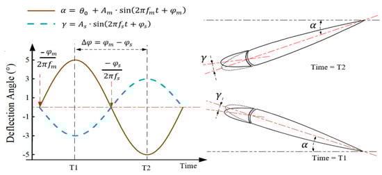
Figure 18.
Schematic diagram of deflections for the airfoil with active leading edge.
The angle of attack of the main airfoil is set as the reference. As illustrated in Figure 18, when the phase of the main airfoil is set at 0°, the airfoil executes oscillating deflections following an upward–downward sequence. At the same time, the phase of the leading edge is set at 180°, resulting in a phase difference ° between the leading edge and the main airfoil. The deflecting directions of these components become anti-phase.
As shown in Figure 19, independent deflections of the active leading edge have significant effects on aerodynamic loads, especially near stall angles.
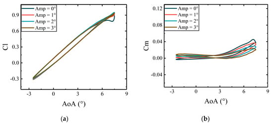
Figure 19.
CFD results of the airfoil aerodynamic coefficients under varying deflection amplitudes of active leading edge: (a) lift coefficients of the whole airfoil; (b) moment coefficients of the whole airfoil.
When the main airfoil deflects to its maximum AoA, flow separation occurs, causing the oscillations in the lift coefficient. Downward deflection of the active leading edge helps to accelerate the flow on the upper surface toward the trailing edge. This delays flow separation and mitigates oscillations in the lift coefficient near stall angles. Meanwhile, the momentum of flow over the airfoil is increased, which reduces the pressure difference between the upper and lower surfaces near the active leading edge. Therefore, the moment coefficient near stall angles has been changed significantly.
The comparisons of the aerodynamic loads between CFD results and calculations from the present model for the airfoil are illustrated in Figure 20, Figure 21 and Figure 22. Variations of deflection amplitudes of the active leading edge were taken into account.
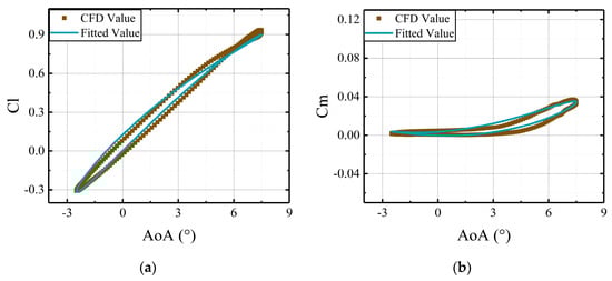
Figure 20.
Comparisons of CFD results and the predictions, derived from the aerodynamic model, versus deflections of the main airfoil with the active leading edge deflecting at amplitude of 1°: (a) lift coefficients of the whole airfoil; (b) moment coefficients of the whole airfoil.
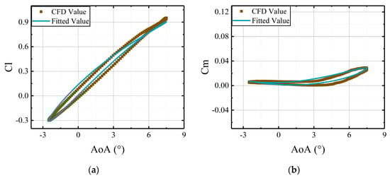
Figure 21.
Comparisons of CFD results and the predictions, derived from the aerodynamic model, versus deflections of the main airfoil with the active leading edge deflecting at amplitude of 2°: (a) lift coefficients of the whole airfoil; (b) moment coefficients of the whole airfoil.
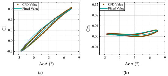
Figure 22.
Comparisons of CFD results and the predictions, derived from the aerodynamic model, versus deflections of the main airfoil with the active leading edge deflecting at amplitude of 3°: (a) lift coefficients of the whole airfoil; (b) moment coefficients of the whole airfoil.
As made evident in Figure 20, Figure 21 and Figure 22, the fitted results from the developed model are in good agreement with the CFD results. Aerodynamic loads of the airfoil with an active leading edge can be calculated accurately by applying the developed aerodynamic model, and the model can capture the variations of deflection amplitudes of the active leading edge.
4.2. Deflection Frequencies of Active Leading Edge
The active leading edge can be designed to suppress the dynamic stall on the retreating side or to reduce vibrations. In that case, the driving frequency of the active leading edge should vary with the rotor rotational speed. The investigations are conducted under different driving frequencies of the active leading edge, and the pitch frequency of the main airfoil is set as the reference. The control parameters governing the main airfoil and the active leading edge are listed in Table 4.
Table 4.
Control parameters in simulations for the airfoil with active leading edge.
Under varying deflection frequencies of the active leading edge, the aerodynamic loads from the developed model are compared to the CFD results. As shown in Figure 22, Figure 23, Figure 24 and Figure 25, aerodynamic loads from the developed model exhibit similar trends to the CFD results. Additionally, it was found that the driving frequency of the active leading edge has considerable influences on the aerodynamic loads of the airfoil.
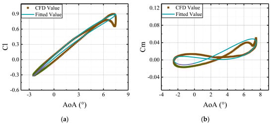
Figure 23.
Comparisons of CFD results and the predictions, derived from the aerodynamic model, versus deflections of the main airfoil with the active leading edge deflecting at frequency of : (a) lift coefficients of the whole airfoil; (b) moment coefficients of the whole airfoil.
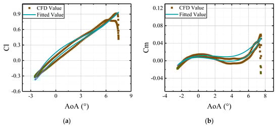
Figure 24.
Comparisons of CFD results and the predictions, derived from the aerodynamic model, versus deflections of the main airfoil with the active leading edge deflecting at frequency of : (a) lift coefficients of the whole airfoil; (b) moment coefficients of the whole airfoil.
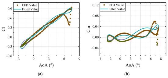
Figure 25.
Comparisons of CFD results and the predictions, derived from the aerodynamic model, versus deflections of the main airfoil with the active leading edge deflecting at frequency of : (a) lift coefficients of the whole airfoil; (b) moment coefficients of the whole airfoil.
The figures reveal that the aerodynamic loads vary nonlinearly with the deflections of airfoil. As shown in Figure 22, Figure 23, Figure 24 and Figure 25, the and curves exhibit a distinct loop, which is attributed to the variations of actuation frequencies of the active leading edge. Therefore, the deflections of the active leading edge can effectively change the aerodynamic loads.
4.3. Deflection Phases of Active Leading Edge
In this section, the deflection phase of the active leading edge is studied for the airfoil with an active leading edge. The phase difference between the deflection of the active leading edge and that of the main airfoil is predefined (° and °). The control parameters governing the main airfoil and active leading edge are listed in Table 5.
Table 5.
Control parameters in simulations for the airfoil with active leading edge.
Under varying deflection phases of the active leading edge, the aerodynamic load calculations from the developed model are compared to the CFD results. As made evident in Figure 22 and Figure 26, the calculated results from the developed model are in agreement with the CFD results. Variations of aerodynamic loads can be captured by this model under different deflections.
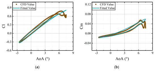
Figure 26.
Comparisons of CFD results and the predictions, derived from the aerodynamic model, versus deflections of the main airfoil with the active leading edge deflecting at phase of 0°: (a) lift coefficients of the whole airfoil; (b) moment coefficients of the whole airfoil.
The phase difference between the leading edge actuation and main airfoil pitch significantly changes the aerodynamic loads with angles of attack. When the main airfoil pitches up to its maximum angle of attack, the active leading edge with a 180° phase difference experiences maximum downward deflection. The variations of phase difference can change the relative positions of the active leading edge at different angles of attack. In that case, the camber of the airfoil can be changed, which affects the unsteady flow around the airfoil. Ultimately, the aerodynamic loads can be influenced.
4.4. The Comparisons of Error Distributions and Computational Efficiency
In this section, the relative errors between results of the proposed model and CFD were calculated under different deflection laws for the airfoil with an active leading edge. The statistics are illustrated in Figure 27 and Figure 28.
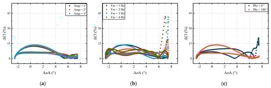
Figure 27.
ΔCl between the CFD results and fitted results: (a) different deflection amplitudes; (b) different deflection frequencies; (c) different deflection phases.
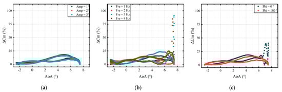
Figure 28.
ΔCm between the CFD results and fitted results: (a) different deflection amplitudes; (b) different deflection frequencies; (c) different deflection phases.
The accuracy of the developed model depends on AoAs and the deflections of the active leading edge. As demonstrated in Figure 27 and Figure 28, under different deflection laws of the airfoil with an active leading edge, relative errors of Cl are below 15%, and those of Cm are below 25% at low AoAs. However, when an airfoil stall occurs, the errors will increase, which means the model is difficult to calculate in terms of the airfoil aerodynamic loads when a stall occurs.
CFD simulations of dynamic cases inherently demand extended computational durations. To verify the efficiency of the developed model, the convergence time for the last cycle of dynamic simulations was quantified. The comparisons of the computational time required for last cycle between the aerodynamic model and CFD are illustrated below. In Figure 29, three deflection laws are considered. Case Numbers 1, 2, and 3 represent three deflection laws, respectively, independent leading edge deflection, main airfoil deflection, and the combined deflections of the main airfoil and active leading edge. In this study, a computer, equipped with an Intel(R) Core (TM) i7-8700 CPU @3.20 GHz, featuring a total of six cores and 32 GB RAM, was employed to perform aerodynamic calculations using both the CFD method and the developed model, respectively.
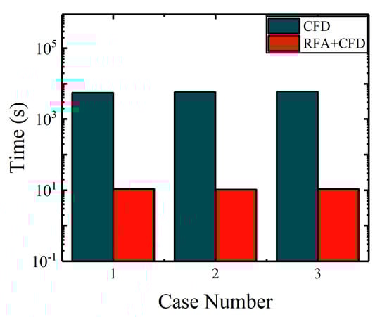
Figure 29.
Comparisons of computational time for selected cases.
As demonstrated in Figure 29, based on the same grids, the statistics of simulations for different deflection laws reveal that the time required for the last cycle of dynamic cases is approximately 1.5 h. On the contrary, under the same conditions, the computational time with the aerodynamic model is about 11 s. Therefore, the developed model significantly improves efficiency in calculating aerodynamic loads for the airfoil with an active leading edge.
The validations of the developed model are performed in this section. The computational results are in good agreement with CFD results under different deflection laws for the airfoil with an active leading edge, except for AoAs near stall. The computational efficiency is significantly enhanced. Therefore, the developed model is more suitable for aeroelastic coupling analysis of rotors equipped with active control devices.
5. Conclusions
A high-efficient aerodynamic model is established in this study, employing the CFD method and RFA approach. The aerodynamic model for the airfoil with an active leading edge is developed. The CFD results are employed to ensure the fidelity of the aerodynamic model. The RFA approach is applied to establish the relationship between the aerodynamic loads and freestream conditions, as well as airfoil motions. The main conclusions are drawn as follows:
- (1)
- For the airfoil with an active leading edge, the CFD method with an overlapping grid approach can simulate the unsteady flow accurately within the narrow gap. The high-fidelity CFD results can be used in the modeling process developed in this study. However, the CFD method is relatively inefficient and time-consuming.
- (2)
- The coefficient matrices of the RFA approach can concisely establish the relationship between aerodynamic loads and airfoil motions. The computational results from the developed model are in good agreement with the CFD results. The identification method can be applied to identify the matrices from the RFA approach, which helps to improve the accuracy of the developed model.
- (3)
- The shapes of components for the airfoil with an active leading edge can be considered in the developed model based on the CFD method. Thus, under reasonable boundary conditions, the model developed in this study can accurately and efficiently calculate the aerodynamic loads for the airfoil with an active leading edge. Compared to the CFD method, the computational efficiency of the model provides a distinct advantage for computationally intensive applications such as the aeroelastic analysis of active rotor.
It should be noted that it is difficult for the model to capture strong nonlinear effects associated with airfoil stall. Therefore, it is necessary to make sure the applicability range of the model is understood before it is employed.
Author Contributions
Conceptualization, J.Z., S.Z. and W.Y.; methodology, J.Z., S.F., S.Z. and W.Y.; writing—original draft preparation, S.F.; writing—review and editing, J.Z.; supervision, J.Z.; project administration, J.Z.; funding acquisition, S.Z. and W.Y. All authors have read and agreed to the published version of the manuscript.
Funding
This research was funded by the Key Laboratory of Rotor Aerodynamics Foundation (RAL202302-6), the National Key Laboratory of Helicopter Aeromechanics Foundation of China (2023-HA-LB-067-03), and the Natural Science Foundation of Jiangsu Province (BK20241420).
Institutional Review Board Statement
Not applicable.
Informed Consent Statement
Not applicable.
Data Availability Statement
Data can be made available upon request from the corresponding authors.
Conflicts of Interest
The authors declare no conflicts of interest.
References
- Friedmann, P.P. On-blade control of rotor vibration, noise, and performance: Just around the corner? J. Am. Helicopter Soc. 2014, 59, 1–37. [Google Scholar] [CrossRef]
- Enenkl, B.; Klöppel, V.; Preißler, D.; Jänker, P. Full scale rotor with piezoelectric actuated blade flaps. In Proceedings of the 28th European Rotorcraft Forum, Bristol, UK, 17–19 September 2002; Royal Aeronautical Society: London, UK, 2002. [Google Scholar]
- Straub, F.K.; Kennedy, D.K.; Stemple, A.D.; Anand, V.R.; Birchette, T.S. Development and whirl tower test of the SMART active flap rotor. In Proceedings of the SPIE-The International Society for Optical Engineering, San Diego, CA, USA, 14–18 March 2004; SPIE: Washington, DC, USA, 2004; pp. 1–11. [Google Scholar] [CrossRef]
- Straub, F.K.; Anand, V.R.; Birchette, T.S.; Lau, B.H. Smart rotor development and wind tunnel test. In Proceedings of the 35th European Rotorcraft Forum, Hamburg, Germany, 22–25 September 2009; DGLR: Berlin, Germany, 2009; pp. 413–434. [Google Scholar]
- Lorber, P.; Neill, J.J.; Hein, B.; Isabella, B.; Andrews, J.; Brigley, M.; Wong, J.; LeMasurier, P.; Wake, B. Whirl and wind tunnel testing of the Sikorsky active flap demonstration rotor. In Proceedings of the 67th American Helicopter Society, Virginia Beach, VA, USA, 3–5 May 2011; AHS International: Fairfax, VA, USA, 2011; pp. 3138–3156. [Google Scholar]
- Dieterich, O.; Enenkl, B.; Roth, D. Trailing edge flaps for active rotor control aeroelastic characteristics of the ADASYS rotor system. In Proceedings of the 62nd American Helicopter Society, Phoenix, AZ, USA, 9–11 May 2006; AHS International: Fairfax, VA, USA, 2006; pp. 964–985. [Google Scholar]
- Stacey, S.; Connolly, N.; Court, P.; Allen, J.; Monteggia, C.; Oliveros, J.M. Leonardo helicopters active rotor programmes to improve helicopter comfort & performance. In Proceedings of the 74th American Helicopter Society, Phoenix, AZ, USA, 14–17 May 2018; Vertical Flight Society: Fairfax, VA, USA, 2018; pp. 2866–2882. [Google Scholar]
- Zhou, J. Research on Vibration Control of Active Rotor with Trailing-Edge Flaps. Ph.D. Thesis, Nanjing University of Aero-nautics and Astronautics, Nanjing, China, 2021. [Google Scholar]
- Jing, S.; Zhao, G.; Gao, Y.; Zhao, Q. Effects of leading edge radius on stall characteristics of rotor airfoil. Aerospace 2024, 11, 470. [Google Scholar] [CrossRef]
- Martin, P.B.; McAlister, K.W.; Chandrasekhara, M.S.; Geissler, W. Dynamic stall measurements and computations for a VR-12 airfoil with a variable droop leading edge. In Proceedings of the AHS International Forum 59, Phoenix, AZ, USA, 6–8 May 2003. [Google Scholar]
- Geissler, W.; Dietz, G.; Mai, H.; Junker, B.; Lorkowski, T. Dynamic stall control investigations on a full size chord blade section. In Proceedings of the 30th European Rotorcraft Forum, Marseilles, France, 14–16 September 2004. [Google Scholar]
- Geissler, W.; Dietz, G.; Mai, H. Dynamic stall on a supercritical airfoil. Aerosp. Sci. Technol. 2005, 9, 390–399. [Google Scholar] [CrossRef]
- Niu, J.; Lei, J.; Lu, T. Numerical research on the effect of variable droop leading-edge on oscillating NACA 0012 airfoil dynamic stall. Aerosp. Sci. Technol. 2018, 72, 476–485. [Google Scholar] [CrossRef]
- Mishra, A. A Coupled CFD/CSD Investigation of the Effects of Leading Edge Slat on Rotor Performance. Ph.D. Thesis, University of Maryland, College Park, MD, USA, 2021. [Google Scholar]
- Mishra, A.; Baeder, J.D. Coupled aeroelastic prediction of the effects of leading-edge slat on rotor performance. J. Aircr. 2016, 53, 141–157. [Google Scholar] [CrossRef]
- Wang, H.; Jiang, X.; Chao, Y.; Li, Q.; Li, M.; Zheng, W.; Chen, T. Effects of leading edge slat on flow separation and aerodynamic performance of wind turbine. Energy 2019, 182, 988–998. [Google Scholar] [CrossRef]
- Yeo, H.; Bosworth, J.; Acree, C.W., Jr.; Kreshock, A.R. Comparison of CAMRAD II and RCAS predictions of tiltrotor aeroelastic stability. In Proceedings of the 73rd American Helicopter Society, Fort Worth, TX, USA, 9–11 May 2017. [Google Scholar]
- Saberi, H.; Hasbun, M.; Hong, J.Y.; Yeo, H.; Ormiston, R.A. Overview of RCAS capabilities, validations, and rotorcraft applications. In Proceedings of the 71st American Helicopter Society, Virginia Beach, VA, USA, 5–7 May 2015. [Google Scholar]
- Shen, J. Comprehensive Aeroelastic Analysis of Helicopter Rotor with Trailing-Edge Flap for Primary Control and Vibration Control. Ph.D. Thesis, University of Maryland, College Park, MD, USA, 2003. [Google Scholar]
- Kim, J. Design and Analysis of Rotor Systems with Multiple Trailing Edge Flaps and Resonant Actuators. Ph.D. Thesis, The Pennsylvania State University, University Park, PA, USA, 2005. [Google Scholar]
- Myrtle, T.F.; Friedmann, P.P. Application of a new compressible time domain aerodynamic model to vibration reduction in helicopters using an actively controlled flap. In Proceedings of the 24th European Rotorcraft Forum, Marseilles, France, 15–17 September 1998. [Google Scholar]
- Liu, L.; Friedmann, P.P.; Padthe, A.K. An approximate unsteady aerodynamic model for flapped airfoils including improved drag predictions. In Proceedings of the 34th European Rotorcraft Forum, Liverpool, UK, 16–19 September 2008. [Google Scholar]
- Liu, L.; Padthe, A.K.; Friedmann, P.P. Computational study of Microflaps with application to vibration reduction in helicopter rotors. AIAA J. 2011, 49, 1450–1465. [Google Scholar] [CrossRef]
- Padthe, A.K.; Liu, L.; Friedmann, P.P. A comprehensive study of active Microflaps for vibration reduction in rotorcraft. In Proceedings of the 66th American Helicopter Society, Phoenix, AZ, USA, 11–13 May 2010. [Google Scholar]
- Tiffany, S.H.; Adams, W.M. Nonlinear Programming Extensions to Rational Function Approximation Methods for Unsteady Aerodynamic Forces; NASA TP-2776; NASA: Washington, DC, USA, 1988.
- Rogers, K.L. Airplane Math Modeling Methods for Active Control Design; AGARD CP-228; NASA: Washington, DC, USA, August 1977; pp. 1–11.
- Hsieh, W.W. Nonlinear multivariate and time series analysis by neural network methods. Rev. Geophys. 2004, 42, 1–25. [Google Scholar] [CrossRef]
- Spaid, F.W. High Reynolds number, multielement airfoil flowfield measurements. J. Aircr. 2000, 37, 499–507. [Google Scholar] [CrossRef]
- Pascioni, K.A.; Cattafesta, L.N.; Choudhari, M.M. An experimental investigation of the 30P30N multi-element high-lift airfoil. In Proceedings of the 20th AIAA/CEAS Aeroacoustics Conference (35th AIAA Aeroacoustics Conference), Atlanta, GA, USA, 16–20 June 2014. [Google Scholar] [CrossRef]
- McCroskey, W.J.; McAlister, K.W.; Carr, L.W.; Pucci, S.L. An Experimental Study of Dynamic Stall on Advanced Airfoil Sections Volume 1: Summary of the Experiment; NASA TM-84245; NASA: Washington, DC, USA, 1982.
Disclaimer/Publisher’s Note: The statements, opinions and data contained in all publications are solely those of the individual author(s) and contributor(s) and not of MDPI and/or the editor(s). MDPI and/or the editor(s) disclaim responsibility for any injury to people or property resulting from any ideas, methods, instructions or products referred to in the content. |
© 2025 by the authors. Licensee MDPI, Basel, Switzerland. This article is an open access article distributed under the terms and conditions of the Creative Commons Attribution (CC BY) license (https://creativecommons.org/licenses/by/4.0/).