Linear Gauss Pseudospectral Method Using Neighboring Extremal for Nonlinear Optimal Control Problems

Abstract

This article proposes a method to solve nonlinear optimal control problems with arbitrary performance indices and terminal constraints, which is based on the neighboring extremal method and Gauss pseudospectral collocation. Firstly, a quadratic performance index is formulated, which minimizes the second-order variation of the nonlinear performance index and fully considers the deviations in initial states and terminal constraints. Secondly, the first-order necessary conditions are applied to derive the perturbation differential equations involving deviations in state and costate variables. Therefore, a quadratic optimal control problem is formulated, which is subject to such perturbation differential equations. Thirdly, the Gauss pseudospectral collocation is used to transform the differential and integral operators into algebraic operations. Therefore, an analytical solution of the control correction can be successfully derived in the polynomial space, which comes close to the optimal solution. This method has a fast computation speed and low computational complexity due to the discretization at orthogonal points, making it suitable for online applications. Finally, some simulations and comparisons with the optimal solution and other typical methods have been carried out to evaluate the performance of the method. Results show that it not only performs well in computational efficiency and accuracy but also has great adaptability and optimality. Moreover, Monte Carlo simulations have been conducted. The results demonstrate that it has strong robustness and excellent performance even in highly dispersed environments.

1. Introduction

The optimal control theory has been widely studied since its first appearance. It has been applied in mechanical [1], aerospace [2], chemical [3], and other engineering fields through continuous development. In the aerospace field, numerous complicated and critical problems can be described in the form of optimal control problems (OCPs), which include attitude control [4] and trajectory optimization [5,6]. As the complexity of problems increases, previous optimal control methods face challenges in providing rapid and accurate solutions, particularly when computational resources are limited. Therefore, it is necessary to study more efficient and innovative solving methods.

In recent years, the pseudospectral method has become an important method to solve nonlinear OCPs, owing to its high computational accuracy and fast convergence [7,8,9,10,11]. The pseudospectral method, as a direct method, approximates global state and control variables with orthogonal polynomials, thereby transforming the differential equations into a set of linear algebraic equations. In addition to the various constraints and performance indices after transformation, the original nonlinear optimal control problem can be transformed into a nonlinear programming (NLP) problem, which can be solved using mature nonlinear optimization solvers such as SNOPT and IPOPT [12,13,14,15,16,17,18]. Moreover, the pseudospectral method has some great characteristics, such as accurate estimation of the costates, the equivalence between the first-order necessary condition of the transformed NLP problem and the Karush–Kuhn–Tucker (KKT) condition of the original OCP [19,20], and a well-established convergence proof [21]. Pseudospectral methods are categorized into the Legendre Pseudospectral Method (LPM), Gauss pseudospectral method (GPM), Radau pseudospectral method (RPM), and Chebyshev Pseudospectral Method (CPM) according to different orthogonal polynomial collocations [22,23]. However, NLP solvers consume significant memory and computational resources, and they cannot guarantee the feasibility of each step in the computation process. Additionally, if the initial guess provided is not sufficiently accurate, the computational time cannot be guaranteed within a specified limit. Therefore, the pseudospectral method is suitable for offline optimization [24,25].

In order to solve the nonlinear OCP online, Padhi et al. proposed a method for solving finite-time nonlinear OCPs with terminal constraints, known as model predictive static programming (MPSP), combining the idea of nonlinear model predictive control (MPC) and approximate dynamic programming [26]. This method predicts terminal errors through numerical integration and discretization dynamics using the Euler integration. It has been successfully applied to many problems in the aerospace field [27,28]. However, this approach requires a large number of nodes to ensure the computational accuracy, which leads to low computational efficiency. Yang et al. also proposed a linear Gauss pseudospectral model predictive control method (LGPMPC) on the framework of MPC, which can solve the nonlinear OCP with fixed time [29]. In comparison with MPSP, this method employs orthogonal collocation points, requiring fewer nodes for the same accuracy, and only needs to solve linear algebraic equations through linearization, which has higher computational efficiency and can be applied online. This method has also been developed and applied in various scenarios such as reentry guidance [30] and long-term air-to-air missile guidance [31,32]. Also, scholars use a pseudospectral discretization strategy to reduce the requirement of the number of nodes for MPSP [33]. However, both of the above methods require a performance index in the form of linear quadratic, and their costate variables are not the same as those of the original OCP. Therefore, they cannot solve OCPs with arbitrary performance indices or provide the costate variables of the original problem.

Convex optimization methods have also been widely applied in the field of guidance control due to their global optimality and convergence properties. Tang et al. proposed an optimization scheme for solving the fuel-optimal control problem by combining the indirect method with the successive convex programming [34]. Wang et al. proposed improved sequential convex programming algorithms based on line-search and trust-region methods to address constrained entry trajectory optimization problems [35]. Some researchers have also studied the combination of pseudospectral methods and convex optimization to improve accuracy. Sagliano investigated the Mars-powered descent problem using the pseudospectral convex optimization method [36]. Li et al. combined Chebyshev pseudospectral discretization with successive convex optimization to propose an online guidance method, which was applied to orbit transfer problems [37]. However, the use of convex optimization methods requires problem convexification, and the inner iterations of sequential convex optimization consume significant computational resources. The online computational efficiency of this method needs to be further improved.

The neighboring extremal optimal method was proposed in the 1960s [38,39], which can obtain the feedback correction when the parameters of the OCP are disturbed. Given the precalculated nominal optimal solution, this method can provide a first-order approximation of the optimal solution for perturbations in initial states and terminal constraints by minimizing the quadratic variation of the performance index. Typically, this method employs a Riccati transformation and backward sweep to solve the linearized quadratic problem derived from the original problem, yielding linear feedback gains [40,41]. However, due to the necessity of solving the Riccati matrix differential equations formed during the backward sweep process, the computational efficiency is too low to be applied online. In recent years, many scholars have focused on improving the computational efficiency of the neighboring extremal method [42,43,44,45,46].

Inspired by LGPMPC and the neighboring extremal method, this paper proposes an efficient algorithm to solve nonlinear OCPs online with arbitrary performance indices. It is referred to as the neighboring extremal linear Gauss pseudospectral method (NELGPM). The main contributions of this paper are as follows: Firstly, the deviations in initial states and terminal constraints are fully considered. A quadratic performance index involving the second-order variation of the original nonlinear performance index is formulated through the variational principle and linearization around the nominal optimal solution. Secondly, the perturbation differential equations involving the deviations between the neighboring extremal path and the original optimal solution are derived via the first-order necessary conditions. Then, an OCP with a quadratic performance index and boundary constraints is formulated. Thirdly, the Gauss pseudospectral collocation is utilized to discretize the quadratic OCP, thereby transforming it into a set of linear algebraic equations including deviations in state and costate variables. Furthermore, on the polynomial space, an analytical solution of the control correction can be successfully derived to come close to the nonlinear optimal solution for the original OCP. Because of discretization at orthogonal points, this process is characterized by high computation speed and low computational complexity, which makes it suitable for online applications. The main difference from previous work is that the proposed method can solve OCP with an arbitrary performance index and provide costate information of optimal control, which greatly expands the scope of applications. Finally, the terminal guidance problem is applied to verify the performance of the proposed method. Some simulations and comparisons have been performed. The results show that it has not only high computational efficiency and accuracy, but also optimality for an arbitrary performance index. Additionally, Monte Carlo simulations have been carried out. The results demonstrate that the proposed method, even in highly dispersed environments, has good adaptability and robustness. Furthermore, NELGPM has great potential for real-time online applications.

The chapters of this paper are organized as follows: Section 2 and Section 3 introduce the problem formulation and the theory of neighboring extremal optimal control. Next, the solving process of pseudospectral discretization and the derivation of the control correction formula are described in detail. Section 4 is the simulation and discussion, and Section 5 presents the conclusion.

2. Problem Formulation

For an OCP with fixed terminal time and terminal constraints, the state differential equations are given by

$$\dot{x}=f\left(x,u,t\right)$$

(1)

where $x\in R^n$ is the state vector, $u\in R^m$ is the control vector, and $t\in R$ is the time variable.

And terminal constraints are

$$\psi \left[x\left(t_f\right)\right]=\left[\begin{array}{c}{x}_1\left(t_f\right)-x_{1f}\hfill \\ ⋮\hfill \\ x_q\left(t_f\right)-x_{qf}\hfill \end{array}\right]=0$$

(2)

where $0\le q\le n$ is the number of fixed state variables at the terminal, $x_{1f},\dots ,x_{qf}$ are the fixed terminal values, and $t_f$ is the terminal time and is also fixed.

The performance index is

$$J=\varphi \left[x\left(t_f\right)\right]+{\int }_{t_0}^{t_f}L\left[x\right(t),u(t),t]dt$$

(3)

where $t_0$ is the initial time, $x\left(t_0\right)$ is the initial state, and $\varphi$ and L are known scalar functions. Equations (1)–(3) describe a general fixed-time OCP, which is to identify a set of control variables $u\left(t\right)$ that minimize the performance index J.

For the OCP as above, it is known from the optimal control theory that the optimal solution is determined by the following first-order necessary conditions. The Hamiltonian function H can be expressed as

$$H=L+{\lambda }^{T}f$$

(4)

where $\lambda$ is the costate vector. State equations, costate equations, and control equations are

$$\begin{array}{c}\dot{x}={\displaystyle \frac{\mathsf{\partial }H}{\mathsf{\partial }\lambda }}\\ \dot{\lambda }=-{\displaystyle \frac{\mathsf{\partial }H}{\mathsf{\partial }x}}\\ 0={\displaystyle \frac{\mathsf{\partial }H}{\mathsf{\partial }u}}\end{array}$$

(5)

The transversality conditions are

$$\lambda \left(t_f\right)={\left({\displaystyle \frac{\mathsf{\partial }\varphi }{\mathsf{\partial }x}}+{\displaystyle \frac{\mathsf{\partial }{\psi }^T}{\mathsf{\partial }x}}\nu \right)}_{t=t_f}$$

(6)

where $\nu$ is the Lagrange multiplier associated with the terminal constraints. According to (2) and (6), if the variable $x_i\left(t_f\right)(q+1\le i\le n)$ is not terminally constrained, then

$${\lambda }_i\left(t_f\right)={\left[{\varphi }_x\right]}_{t_f}$$

(7)

where ${\varphi }_x={\displaystyle \frac{\mathsf{\partial }\varphi }{\mathsf{\partial }x}}$. If the variable $x_i\left(t_f\right)(0\le i\le q)$ is terminally constrained, then

$${\lambda }_i\left(t_f\right)={[{\varphi }_x+{\nu }_i]}_{t_f}$$

(8)

The solution to the original OCP can be obtained by solving the two-point boundary value problem (TPBVP) consisting of this set of equations and boundary conditions. However, if the problem is nonlinear, it is very difficult to solve in an analytical manner. Moreover, numerical iterative methods are typically used to solve such problems.

3. Neighboring Extremal Linear Gauss Pseudospectral Method

3.1. Neighboring Extremal Optimal Control

It is known that the optimal solution for a general OCP varies with changes in initial states and terminal conditions. On the assumption of small disturbances, the neighboring extremal method can provide the solution approaching the optimal solution for the problem when the initial states and terminal conditions are changed.

Considering differential equation constraints (1) and terminal constraints (2), the augmented performance index can be expressed as

$$\overline{J}=\varphi \left[x\left(t_f\right)\right]+{\nu }^T\psi \left[x\left(t_f\right)\right]+{\int }_{t_0}^{t_f}[H(x,u,\lambda ,t)-{\lambda }^T\dot{x}]dt$$

(9)

Considering the initial state deviations $\delta x\left(t_0\right)$ and terminal deviations $\delta \psi \left(t_f\right)$, the increment of $\overline{J}$ with respect to changes in control $\delta u$ can be expressed as

$$\begin{array}{c}\Delta \overline{J}={\left[{\Phi }_x\delta x+{\displaystyle \frac{1}{2}}\delta x^T{\Phi }_{xx}\delta x+{\nu }^T\delta \psi \right]}_{t=t_f}-{\left[{\lambda }^T\delta x\right]}_{t_0}^{t_f}+{\int }_{t_0}^{t_f}\left({\dot{\lambda }}^T\delta x+H_x\delta x+H_u\delta u\right.\\ \left.+{\displaystyle \frac{1}{2}}\delta x^T{H}_{xx}\delta x+{\displaystyle \frac{1}{2}}\delta x^T{H}_{xu}\delta u+{\displaystyle \frac{1}{2}}\delta u^T{H}_{ux}\delta x+{\displaystyle \frac{1}{2}}\delta u^T{H}_{uu}\delta u\right)dt+o(·)\end{array}$$

(10)

where $\Phi =\varphi +{\nu }^T\psi$, ${\left(\right)}_x={\displaystyle \frac{\mathsf{\partial }\left(\right)}{\mathsf{\partial }x}}$, ${\left(\right)}_{xx}={\displaystyle \frac{{\mathsf{\partial }}^2\left(\right)}{\mathsf{\partial }{x}^2}}$, ${\left(\right)}_{x\mathrm{u}}={\displaystyle \frac{{\mathsf{\partial }}^2\left(\right)}{\mathsf{\partial }x\mathsf{\partial }u}}$, etc. Because of the approximation around the nominal optimal solution, the coefficients satisfy the previous first-order necessary conditions. So (10) can be simplified to

$$\begin{array}{c} \Delta \overline{J}={\left({\lambda }^T\delta x\right)}_{t=t_0}+{\left({\nu }^T\delta \psi \right)}_{t=t_f}+{\left({\displaystyle \frac{1}{2}}\delta x^T{\Phi }_{xx}\delta x\right)}_{t=t_f}\\ {\displaystyle +\frac{1}{2}{\int }_{t_0}^{t_f}\left[\begin{array}{cc}\delta x^T& \delta u^T\end{array}\right]\left[\begin{array}{cc}{H}_{xx}& H_{xu}\\ H_{ux}& H_{uu}\end{array}\right]\left[\begin{array}{c}\delta x\\ \delta u\end{array}\right]dt}\end{array}$$

(11)

where all the coefficients are calculated according to the optimal solution.

From (11), it can be seen that ${\lambda }^T\left(t_0\right)$ and ${\nu }^T$ are the first-order functions of the performance index J with respect to the initial state deviations $\delta x\left(t_0\right)$ and terminal deviations $\delta \psi \left(t_f\right)$.

$${\delta }^2\overline{J}={\displaystyle \frac{1}{2}}{\left[\delta x^T{\Phi }_{xx}\delta x\right]}_{t=t_f}+{\displaystyle \frac{1}{2}}{\int }_{t_0}^{t_f}\left[\begin{array}{cc}\delta x^T& \delta u^T\end{array}\right]\left[\begin{array}{cc}{H}_{xx}& H_{xu}\\ H_{ux}& H_{uu}\end{array}\right]\left[\begin{array}{c}\delta x\\ \delta u\end{array}\right]dt$$

(12)

The second-order terms on the right-hand side of (11) can be interpreted as the second-order variation of the original problem, which can be seen as solving a new OCP with a quadratic performance index (12), that is, by selecting $\delta u\left(t\right)$ to obtain the neighboring extremal path whose initial and terminal conditions are slightly different from the optimal path. The neighboring extremal path satisfies the following linear perturbation equation:

$$\delta \dot{x}=f_x\delta x+f_u\delta u$$

(13)

The coefficients of this equation are also calculated according to the original optimal solution. The boundary conditions for this new OCP are

$$\begin{array}{c}\delta x\left(t_0\right)=\delta x_0\end{array}$$

(14)

$$\begin{array}{c}{\left[{\psi }_x\delta x\right]}_{t=t_f}=\delta {\psi }_f\end{array}$$

(15)

Considering the differential equation constraints (13) and terminal constraints (15), the new augmented performance index can be expressed as

$$\begin{array}{c}{\overline{J}}_1={\left({\lambda }^T\delta x\right)}_{t=t_0}+{\left({\nu }^T\delta \psi \right)}_{t=t_f}+{\displaystyle \frac{1}{2}}{\left[\delta x^T{\Phi }_{xx}\delta x\right]}_{t=t_f}+d{\nu }^T{\left[{\psi }_{x}dx\right]}_{t=t_f}\\ +{\int }_{t_0}^{t_f}\left\{{\displaystyle \frac{1}{2}}\left[\begin{array}{cc}\delta x^T& \delta u^T\end{array}\right]\left[\begin{array}{cc}{H}_{xx}& H_{xu}\\ H_{ux}& H_{uu}\end{array}\right]\left[\begin{array}{c}\delta x\\ \delta u\end{array}\right]\right\}dt-\left\{\delta {\lambda }^T\left(\delta \dot{x}-f_x\delta x-f_u\delta u\right)\right\}dt\end{array}$$

(16)

where $d\nu$ and $\delta \lambda$ are the deviations of the Lagrange multipliers in the original problem. Now fixing initial state deviations $\delta x\left(t_0\right)$ and terminal deviations $\delta \psi \left(t_f\right)$, the increment of ${\overline{J}}_1$ with respect to ${\delta }^{2}x$ and ${\delta }^{2}u$ is expressed as follows:

$$\begin{array}{c}\Delta {\overline{J}}_1={\left[\left(\delta x^T{\Phi }_{xx}+d{\nu }^T{\psi }_x-\delta {\lambda }^T\right){\delta }^{2}x\right]}_{t=t_f}\\ +{\int }_{t_0}^{t_f}\left[\left(\delta \dot{\lambda }+\delta x^T{H}_{xx}+\delta {\lambda }^T{f}_x+\delta u^T{H}_{ux}\right){\delta }^{2}x\right.\\ \left.+\left(\delta x^T{H}_{xu}+\delta {\lambda }^T{f}_u+\delta u^T{H}_{uu}\right){\delta }^{2}u\right]dt+o(·)\end{array}$$

(17)

Neglecting high-order terms in (17), we can obtain the necessary condition for the new OCP.

$$\begin{array}{c}\delta \dot{\lambda }=-H_{xx}\delta x-f_x^T\delta \lambda -H_{xu}\delta u\end{array}$$

(18)

$$\begin{array}{c}\delta \lambda \left(t_f\right)={[({\varphi }_{xx}+v^T{\psi }_{xx})\delta x+{\psi }_x^{T}d\nu ]}_{t=t_f}\end{array}$$

(19)

$$\begin{array}{c}{H}_{ux}\delta x+f_u^T\delta \lambda +H_{uu}\delta u=0\end{array}$$

(20)

The linear TPBVP formed by Equations (18)–(20) and (13)–(15) determines the neighboring extremal path with given initial state deviations and terminal deviations. From the above derivations, it can be inferred that the solutions to the TPBVP can minimize (or maximize) the second-order variation of the original OCP. As indicated by (11), the first-order deviation terms are independent of control variables. However, changes in control derived from the second-order deviation terms yield the optimal adjustments. Assuming $H_{uu}$ is nonsingular, the control updates can be represented as follows:

$$\delta u\left(t\right)=-H_{uu}^{-1}(H_{ux}\delta x+f_u^T\delta \lambda )$$

(21)

According to Legendre’s condition, the second-order variation takes the minimum value if $H_{uu}>0$. When $H_{uu}>0$, $H_{uu}$ is nonsingular. Substituting (21) into (13) and (18) yields a set of differential equations only related to $\delta x$ and $\delta \lambda$, expressed as follows:

$$\begin{array}{cc}\hfill \delta \dot{x}& =A\left(t\right)\delta x-B\left(t\right)\delta \lambda \hfill \\ \hfill \delta \dot{\lambda }& =-C\left(t\right)\delta x-A^T\left(t\right)\delta \lambda \hfill \end{array}$$

(22)

where

$$\begin{array}{cc}\hfill A\left(t\right)& =f_x-f_u{H}_{uu}^{-1}{H}_{ux}\hfill \\ \hfill B\left(t\right)& =f_u{H}_{uu}^{-1}{f}_u^T\hfill \\ \hfill C\left(t\right)& =H_{xx}-H_{xu}{H}_{uu}^{-1}{H}_{ux}\hfill \end{array}$$

(23)

The boundary conditions are as shown in (24).

$$\begin{array}{c}\delta x\left(t_0\right)=\delta x_0\hfill \\ \delta \lambda \left(t_f\right)={[({\varphi }_{xx}+v^T{\psi }_{xx})\delta x+{\psi }_x^{T}d\nu ]}_{t=t_f}\hfill \\ \delta \psi ={\left[{\psi }_x\delta x\right]}_{t=t_f}\hfill \end{array}$$

(24)

In the past, the conventional approach for solving the aforementioned linear TPBVP was the backward sweep method. Actually, the backward sweep method requires multiple numerical integrations, including solving a set of Riccati matrix differential equations. Additionally, to ensure accuracy and numerical stability, it also requires a sufficiently large number of integration nodes. These restrict the application of the neighboring extremal method. In response, this paper proposes a new method for efficiently solving this problem after linearization in polynomial space.

3.2. Pseudospectral Collocation Scheme of NELGPM

For the perturbed differential Equation (22), the linear Gauss pseudospectral discretization strategy is used to discretize it and transform it into a set of linear equations, so that the changes in state variables and costate variables at each discrete node can be solved efficiently. Then the correction of control variables can be calculated from (21) to correct the disturbance.

Gaussian quadrature is a widely used integration method, known for its high computational accuracy with few nodes. In this method, the supporting nodes are the zeros of orthogonal polynomials. In this paper, we utilize a Legendre-type Gaussian quadrature, whose zeros range within $[-1,1]$. Thus, the initial step involves transforming the original problem’s time domain from $[t_0,t_f]$ to $[-1,1]$. The transformation formula is as follows:

$$t={\displaystyle \frac{t_f-t_0}{2}}\tau +{\displaystyle \frac{t_f+t_0}{2}}$$

(25)

The performance index and Hamiltonian function are also transformed into the new time domain, yielding the following outcomes:

$$J=\varphi \left[x\left(1\right)\right]+{\displaystyle \frac{t_f-t_0}{2}}{\int }_{-1}^{1}L\left[x\right(\tau ),u(\tau ),\tau ]d\tau$$

(26)

$$H[x\left(\tau \right),u\left(\tau \right),\tau ]=L[x\left(\tau \right),u\left(\tau \right),\tau ]+{\lambda }^{T}f[x\left(\tau \right),u\left(\tau \right),\tau ]$$

(27)

Equation (22) is also transformed into the following form:

$$\left[\begin{array}{c}\delta \dot{x}\\ \delta \dot{\lambda }\end{array}\right]={\displaystyle \frac{t_f-t_0}{2}}\left[\begin{array}{cc}A& -B\\ -C& -A^T\end{array}\right]\left[\begin{array}{c}\delta x\\ \delta \lambda \end{array}\right]$$

(28)

As stated above, the discrete nodes are chosen as the zeros of orthogonal polynomials. Let the order of the orthogonal polynomials be N, and ${\tau }_l$ ($l=1,2,\dots ,N$) are the zeros of the Nth-order Legendre orthogonal polynomials, also known as LG (Legendre–Gauss) nodes. From these zeros, two sets of Nth-order Lagrange polynomials $L_N\left(\tau \right)$ and $L_N^{\ast }\left(\tau \right)$ can be obtained, which exhibit a certain conjugate relationship.

$$\begin{array}{c}\delta x^N\left(\tau \right)={\displaystyle \sum _{l=0}^N}{L}_l\left(\tau \right)\delta x\left({\tau }_l\right)\\ \delta u^N\left(\tau \right)={\displaystyle \sum _{l=0}^N}{L}_l\left(\tau \right)\delta u\left({\tau }_l\right)\\ \delta {\lambda }^N\left(\tau \right)={\displaystyle \sum _{l=1}^{N+1}}{L}_l^{\ast }\left(\tau \right)\delta \lambda \left({\tau }_l\right)\end{array}$$

(29)

Consequently, the variations in state variables, control variables, and costate variables can be expressed through Lagrange interpolation polynomials as shown in (29), where $\delta x\left({\tau }_l\right)$, $\delta u\left({\tau }_l\right)$, and $\delta \lambda \left({\tau }_l\right)$ represent the respective variable values at the discrete nodes and $\delta x^N$, $\delta u^N$, and $\delta {\lambda }^N$ represent the result after using the Nth-order Lagrange interpolation polynomial.

From the Lagrange interpolation polynomial, we can obtain

$$L_l\left({\tau }_k\right)=\left\{\begin{array}{cc}1& l=k\\ 0& l\ne k\end{array}\right.,L_l^{\ast }\left({\tau }_k\right)=\left\{\begin{array}{cc}1& l=k\\ 0& l\ne k\end{array}\right.$$

(30)

It is obvious that the Lagrange polynomials satisfy the requirements at the interpolation nodes.

$$\begin{array}{c}\delta x^N\left({\tau }_l\right)=\delta x\left({\tau }_l\right)\\ \delta u^N\left({\tau }_l\right)=\delta u\left({\tau }_l\right)\\ \delta {\lambda }^N\left({\tau }_l\right)=\delta \lambda \left({\tau }_l\right)\end{array}$$

(31)

Upon differentiating the Lagrange interpolation polynomials (29) at the discrete nodes, the expressions for the derivatives of the change in state variables and costate variables at the LG nodes are obtained as follows:

$$\begin{array}{c}\delta {\dot{x}}^N\left({\tau }_k\right)={\displaystyle \sum _{l=0}^N}{D}_{kl}\delta x\left({\tau }_l\right)\\ \delta {\dot{\lambda }}^N\left({\tau }_k\right)={\displaystyle \sum _{l=1}^{N+1}}{D}_{kl}^{\ast }\delta \lambda \left({\tau }_l\right)\end{array}$$

(32)

where $l=0,1,\dots ,N$, $k=1,2,\dots ,N$. Simultaneously, this process also yields a differential approximation matrix $D_{kl}$ of size $N\times (N+1)$. D and $D^{\ast }$ possess a certain adjoint relationship, which can be determined through the following formula:

$$D_{kl}=\sum _{i=0,i\ne l}^N{\displaystyle \frac{{\displaystyle \prod _{j=0,j\ne i,l}^N}({\tau }_k-{\tau }_j)}{{\displaystyle \prod _{j=0,j\ne l}^N}({\tau }_l-{\tau }_j)}},D_{lk}^{\ast }=-{\displaystyle \frac{{\omega }_k}{{\omega }_l}}{D}_{kl},{\overline{D}}_k=-\sum _{l=1}^N{D}_{kl}$$

(33)

where ${\omega }_k$ and ${\omega }_l$ are the quadrature coefficients of the Gaussian quadrature formula, and ${\overline{D}}_k$ is the element in the first column of D.

Substituting (32) into (28), and incorporating the relationship between the initial and terminal deviations yields the following set of linear algebraic equations:

$$\begin{array}{c}{\displaystyle \sum _{l=0}^N}{D}_{kl}\delta x_l-{\displaystyle \frac{t_f-t_0}{2}}\left(A_k\delta x_k-B_k\delta {\lambda }_k\right)=0\\ -{\displaystyle \frac{t_f-t_0}{2}}{\displaystyle \sum _{k=1}^N}{\omega }_k\left(A_k\delta x_k-B_k\delta {\lambda }_k\right)=\delta x_0-\delta x_{N+1}\\ {\displaystyle \sum _{l=1}^{N+1}}{D}_{kl}^{\ast }\delta {\lambda }_l+{\displaystyle \frac{t_f-t_0}{2}}\left(C_k\delta x_k+A_k^T\delta {\lambda }_k\right)=0\\ \delta {\lambda }_0=\delta {\lambda }_{N+1}+{\displaystyle \frac{t_f-t_0}{2}}{\displaystyle \sum _{k=1}^N}{\omega }_k\left(C_k\delta x_k+A_k^T\delta {\lambda }_k\right)\end{array}$$

(34)

where $k=1,2,\dots ,N$. $A_k$, $B_k$ and $C_k$ represent the values of the A, B, and C matrices at the k-th node. Note that the boundary nodes are not all included in the dynamic constraints. Therefore, two additional constraints are added to (34), so that the terminal state deviations and costate deviations satisfy the dynamic equation constraints through Gaussian quadrature.

This set of equations shows that there is a certain linear relationship between the state and costate deviations of the neighboring extremal path and the original optimal path, so we can describe the state and costate deviations at all nodes in analytic form and compute the control corrections at all nodes via (21).

3.3. Derivations of Analytical Correction Formula for Control

In this section, we derive the analytical control correction formula to eliminate errors and come close to the optimal solution.

Now define

$$\begin{array}{c}{\mathit{X}}_k=\left[\begin{array}{c}\delta x_k\hfill \\ \delta {\lambda }_k\hfill \end{array}\right]\hfill \\ \mathit{X}={\left[\begin{array}{c}\begin{array}{cccc}{\mathit{X}}_1^T\hfill & {\mathit{X}}_2^T& \dots & {\mathit{X}}_N^T\end{array}\hfill \end{array}\right]}^T\hfill \end{array}$$

(35)

Then we can use $\mathit{X}$ to represent the state and costate deviations at all nodes. In order to obtain the analytical control correction formula, $\mathit{X}$ must first be derived from (34).

The first set of equations from (34) can be written in the following form:

$$\begin{array}{c}{\displaystyle \sum _{l=0}^N}{D}_{kl}\delta x_l=\left[\begin{array}{ccc}{D}_{k1}& \dots & D_{kN}\end{array}\right]\left[\begin{array}{c}\delta x_1\\ ⋮\\ \delta x_N\end{array}\right]+D_{k0}\delta x_0\\ \hspace{1em}\hspace{1em}\hspace{1em}\hspace{1em}\hspace{1em}\hspace{1em}\hspace{1em}={\displaystyle \frac{t_f-t_0}{2}}\left[\begin{array}{cc}{A}_k& -B_k\end{array}\right]\left[\begin{array}{c}\delta x_k\\ \delta {\lambda }_k\end{array}\right]={\displaystyle \frac{t_f-t_0}{2}}{F^{\prime }}_k{\mathit{X}}_k\end{array}$$

(36)

where $k=1,2,\dots ,N$, $F_k^{\prime }=\left[\begin{array}{cc}{A}_k& -B_k\end{array}\right]$. Similarly, the third set of equations from (34) can be expressed as follows:

$$\left[\begin{array}{ccc}{D}_{k1}^{\ast }& \dots & D_{kN}^{\ast }\end{array}\right]\left[\begin{array}{c}\delta {\lambda }_1\\ ⋮\\ \delta {\lambda }_N\end{array}\right]+D_{k(N+1)}^{\ast }\delta {\lambda }_{N+1}={\displaystyle \frac{t_f-t_0}{2}}{F^{″}}_k{\mathit{X}}_k$$

(37)

where $k=1,2,\dots ,N$, $F_k^{″}=\left[\begin{array}{cc}-C_k& -A_k^T\end{array}\right]$. Combining (36) and (37) yields

$$\begin{array}{c}\left[\left[\begin{array}{cc}{D}_{k1}& 0\\ 0& D_{k1}^{\ast }\end{array}\right],\dots ,\left[\begin{array}{cc}{D}_{kN}& 0\\ 0& D_{kN}^{\ast }\end{array}\right]\right]\left[\begin{array}{c}{\mathit{X}}_1\\ ⋮\\ {\mathit{X}}_N\end{array}\right]\\ +\left[\begin{array}{cc}{D}_{k0}& D_{k(N+1)}^{\ast }\end{array}\right]\left[\begin{array}{c}\delta x_0\\ \delta {\lambda }_{N+1}\end{array}\right]={\displaystyle \frac{t_f-t_0}{2}}\left[\begin{array}{c}{F^{\prime }}_k\\ {F^{″}}_k\end{array}\right]{\mathit{X}}_k\end{array}$$

(38)

where $k=1,2,\dots ,N$.

k takes 1 to N, and the N equations in (38) can be simultaneously written as

$$\mathit{DX}+{\mathit{D}}_0\left[\begin{array}{c}\delta x_0\\ \delta {\lambda }_{N+1}\end{array}\right]=\mathit{FX}$$

(39)

where

$$\begin{array}{c}\mathit{D}=\left[\begin{array}{ccc}{D}_{11}^{2s\times 2s}& \dots & D_{1N}^{2s\times 2s}\\ ⋮& \ddots & ⋮\\ D_{N1}^{2s\times 2s}& \dots & D_{NN}^{2s\times 2s}\end{array}\right],{\mathit{D}}_0=\left[\begin{array}{cc}{D}_{10}\hfill & D_{1(N+1)}^{\ast }\\ ⋮\hfill & ⋮\\ D_{N0}\hfill & D_{N(N+1)}^{\ast }\end{array}\right]\\ D_{ij}^{2s\times 2s}=\left[\begin{array}{cc}{D}_{ij}& 0\\ 0& D_{ij}^{\ast }\end{array}\right]\end{array}$$

(40)

$$\mathit{F}={\displaystyle \frac{t_f-t_0}{2}}\left[\begin{array}{ccc}{F}_1& & 0\\ & \ddots & \\ 0& & F_N\end{array}\right],F_k=\left[\begin{array}{c}{F^{\prime }}_k\\ {F^{″}}_k\end{array}\right]$$

(41)

where s represents the number of state variables.

In this way, we convert part of the equations in (34) to the form with $\mathit{X}$ as the unknown quantity, and the remaining one is related to the initial state deviations and the terminal costate deviations.

Combining the second and fourth equations from (34), we obtain

$$\left[\begin{array}{c}\delta x_{N+1}\\ -\delta {\lambda }_0\end{array}\right]=\left[\begin{array}{c}\delta x_0\\ -\delta {\lambda }_{N+1}\end{array}\right]+{\displaystyle \frac{t_f-t_0}{2}}\sum _{k=1}^N\left({\omega }_k{F}_k\left[\begin{array}{c}\delta x_k\\ \delta {\lambda }_k\end{array}\right]\right)$$

(42)

Namely

$$\left[\begin{array}{c}\delta x_{N+1}\\ -\delta {\lambda }_0\end{array}\right]=\left[\begin{array}{cc}{I}_{s\times s}& 0\\ 0& -I_{s\times s}\end{array}\right]\left[\begin{array}{c}\delta x_0\\ \delta {\lambda }_{N+1}\end{array}\right]+\mathit{WX}$$

(43)

where

$$\mathit{W}={\displaystyle \frac{t_f-t_0}{2}}\left[\begin{array}{ccc}{\omega }_1{F}_1& \dots & {\omega }_N{F}_N\end{array}\right]$$

(44)

Equation (43) shows the relationship between the deviations in the initial and terminal times and that in the intermediate discrete nodes.

From (39), if $\mathit{F}-\mathit{D}$ is invertible, we obtain

$$\mathit{X}={\left(\mathit{F}-\mathit{D}\right)}^{-1}{\mathit{D}}_0\left[\begin{array}{c}\delta x_0\\ \delta {\lambda }_{N+1}\end{array}\right]$$

(45)

Substituting (45) into (43) and eliminating the unknown quantity $\mathit{X}$ yields

$$\left[\begin{array}{c}\delta x_{N+1}\\ -\delta {\lambda }_0\end{array}\right]=\left(\left[\begin{array}{cc}{I}_{s\times s}& 0\\ 0& -I_{s\times s}\end{array}\right]+\mathit{W}{\left(\mathit{F}-\mathit{D}\right)}^{-1}{\mathit{D}}_0\right)\left[\begin{array}{c}\delta x_0\\ \delta {\lambda }_{N+1}\end{array}\right]$$

(46)

Define $\mathit{K}=\left[\begin{array}{cc}{I}_{s\times s}& 0\\ 0& -I_{s\times s}\end{array}\right]+\mathit{W}{\left(\mathit{F}-\mathit{D}\right)}^{-1}{\mathit{D}}_0=\left[\begin{array}{cc}{K}_{11}& K_{12}\\ K_{21}& K_{22}\end{array}\right]$, and $K_{11}$, $K_{12}$, $K_{21}$, and $K_{22}$ are s-order submatrices. Then (46) can be simplified to

$$\left[\begin{array}{c}\delta x_{N+1}\\ -\delta {\lambda }_0\end{array}\right]=\left[\begin{array}{cc}{K}_{11}& K_{12}\\ K_{21}& K_{22}\end{array}\right]\left[\begin{array}{c}\delta x_0\\ \delta {\lambda }_{N+1}\end{array}\right]$$

(47)

It is obvious that (47) involves only the deviations in the initial and terminal time. The $\mathit{K}$ is completely determined by the nominal trajectory.

If $K_{12}$ is invertible, the following expressions can be obtained according to (47):

$$\begin{array}{c}\hfill \delta {\lambda }_{N+1}=K_{12}^{-1}\left(\delta x_{N+1}-K_{11}\delta x_0\right)\\ \hfill \delta {\lambda }_0=-K_{21}\delta x_0-K_{22}\delta {\lambda }_{N+1} \end{array}$$

(48)

From the boundary conditions (24), the deviations of terminal state variables $\delta x_{N+1}$ can be calculated via terminal deviations $\delta \psi$. Then, by using (48), the initial and terminal deviations of the costate variables $\delta {\lambda }_0$ and $\delta {\lambda }_{N+1}$ can be obtained. Finally, substituting $\delta x_0$ and $\delta {\lambda }_{N+1}$ into (45), the deviations of state and costate variables $\mathit{X}$ at all discrete nodes can be calculated.

From (35), the values of ${\mathit{X}}_k$ at each node can be obtained. Then substituting ${\mathit{X}}_k$ into (21), the control corrections at all discrete nodes can be obtained as shown in (49).

$$\delta u_k=-H_{uu}^{-1}\left({\tau }_k\right)\left[\begin{array}{cc}{H}_{ux}\left({\tau }_k\right)& f_u^T\left({\tau }_k\right)\end{array}\right]{\mathit{X}}_k$$

(49)

where $k=1,2,\dots ,N$.

Subsequently, through Lagrange interpolation (29), the control corrections $\delta u$ at any given time can be obtained, thereby obtaining the complete control sequence $u\left(t\right)$ for the neighboring extremal path that minimizes the performance index of the original problem under the given initial and terminal deviations.

3.4. Implementation Steps

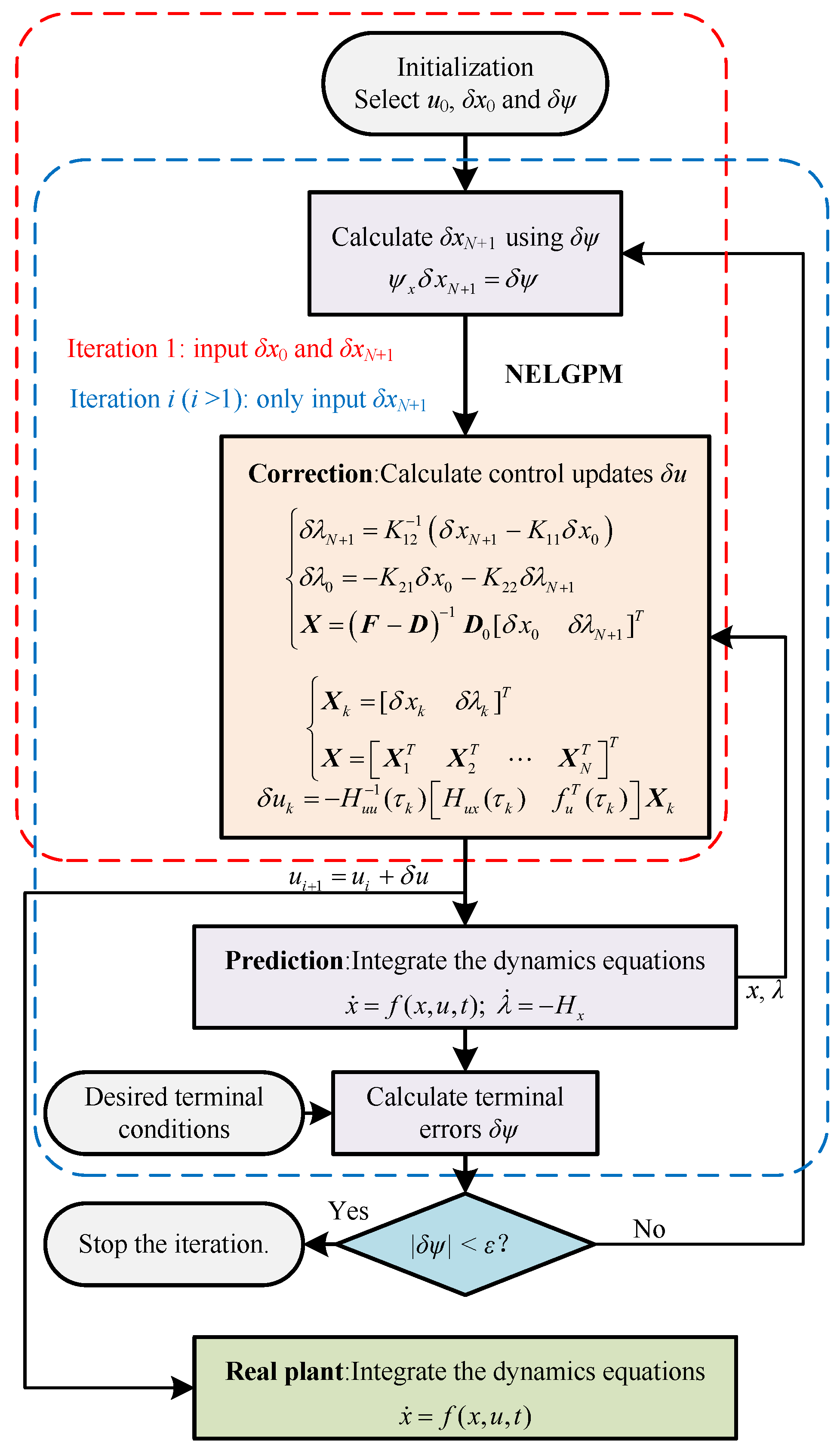
This paper presents the NELGPM for solving the nonlinear optimal control problem with an arbitrary performance index. It iteratively minimizes the second-order variation of the performance index with the constraints on perturbation equations. An analytical solution for this subproblem can be successfully derived in the polynomial space via Gauss pseudospectral collocation. Therefore, it has excellent computational efficiency and accuracy with few discrete points. The implementation steps of the proposed method are demonstrated in Figure 1.

Figure 1. Algorithm Flowchart.

The specific algorithm flow is as follows.

Step 1: Determine the initial optimal trajectory and control, and set the initial state deviations $\delta x_0$ and terminal errors $\delta \psi$.

Step 2: Calculate the terminal state deviations $\delta x_{N+1}$ according to terminal errors $\delta \psi$. Then, based on the standard trajectory, calculate the neighboring extremal control updates from the initial deviations $\delta x_0$ and the terminal deviations $\delta x_{N+1}$ using (45), (48), and (49).

Step 3: Integrate the dynamics differential equations with the updated controls, and record the new trajectory and terminal errors $\delta \psi$.

Step 4: Calculate the terminal state deviations $\delta x_{N+1}$ using the new terminal errors $\delta \psi$. Substitute the terminal state deviations and updated trajectory into (45), (48), and (49) to calculate control updates. At this stage, the initial deviations are set to zero.

Step 5: Take the updated control as the current control and return to step 3. Evaluate whether the terminal error accuracy meets the requirement. If it does, the algorithm terminates; if not, the algorithm continues.

Through the above steps, it can provide the iterative solution coming closer to the optimal solution for the original optimal control problem with the constraints on initial and terminal deviations. It should be noted that the algorithm requires an approximately optimal reference trajectory using the given performance index as the initial trajectory, which can be obtained through offline optimization algorithms.

In addition, according to (23) and (45), the computation of control correction requires some matrices to be nonsingular. Since we need to obtain the optimal solution in advance, the problems chosen for study are all normal optimal control problems. In this case, the matrices generated during the process will not be singular.

4. Numerical Examples

The proposed method was applied to the guidance problem of air-to-ground aircraft. This problem is an OCP with fixed terminal time and terminal constraints. In order to verify the adaptability of the proposed method in different situations, three distinct simulation scenarios were chosen, each sharing identical initial conditions but with different initial state deviations and terminal constraints. Furthermore, the simulation results obtained through the proposed method were compared with those from GPOPS-II, neighboring extremal with backward sweep method (NE + BS), and trajectory shaping guidance (TSG) [47,48]. GPOPS-II, a widely used offline pseudospectral optimization software utilizing the Radau pseudospectral method, served as a benchmark to assess the optimality of the proposed method. The backward sweep method is a classical method for solving the neighboring extremal optimal problem, used to compare and verify the computational efficiency of the proposed method. TSG, a classical terminal guidance law, was employed to ensure angular constraints while guiding the aircraft to the target. All simulations in this paper were carried out in MATLAB R2023b using an AMD Ryzen 7 5800X processor.

4.1. Simulation Model

The employed three degrees of freedom dynamic model [49] is outlined as follows:

$$\begin{array}{c}{\dot{x}}_m=Vcos\gamma cos{\psi }_V\\ \dot{y}=Vcos\gamma cos{\psi }_V\\ \dot{h}=Vsin\gamma \\ \dot{\gamma }={\displaystyle \frac{(a_z-cos\gamma )g}{V}}\\ {\dot{\psi }}_V={\displaystyle \frac{a_{y}g}{Vcos\gamma }}\\ \dot{E}={\displaystyle \frac{V(T-D)}{mg}}\end{array}$$

(50)

where $x_m$, y, h are the position of the aircraft in the Earth-fixed frame and $\gamma$, ${\psi }_V$ are the flight path angle and heading angle. E represents the energy, and the expression is $E=h+{\displaystyle \frac{V^2}{2g}}$. g is the gravitational acceleration. Velocity V can be obtained through the calculation formula of energy. The control variables $a_y$ and $a_z$ act perpendicular to the direction of velocity, while the thrust aligns with the velocity direction.

The formula for calculating the drag D in (50) is as follows, where ${\rho }_0$, $T_0$, L, $S_{ref}$, $C_{D0}$, k are constants, m represents the mass of the aircraft. Since the lift coefficient is approximately proportional to the angle of attack, with a proportionality coefficient of $C_{L\alpha }$, the angle of attack $\alpha$ is computed using (55). Model parameters are listed in Table 1.

$$D={\displaystyle \frac{1}{2}}\rho V^2{S}_{ref}{C}_D$$

(51)

$$\rho ={\rho }_0{\left({\displaystyle \frac{T_0+Lh}{T_0}}\right)}^{-{\displaystyle \frac{g}{LR}}-1}$$

(52)

$$C_D=C_{D0}+k{C}_L^2$$

(53)

$$C_L=2{\displaystyle \frac{mg{(a_y^2+a_z^2)}^{1/2}}{\rho V^2{S}_{ref}}}$$

(54)

$$\alpha ={\displaystyle \frac{C_L}{C_{L\alpha }}}$$

(55)

Table 1. Model parameters.

Parameters	Value	Parameters	Value
${\rho }_0$ (kg/m3)	1.225	k	0.03
T (N)	2000	$C_{L\alpha }$	50
L (K/m)	−0.0065	m (kg)	500
$S_{ref}$ (m2)	0.132	$T_0$ (K)	288.16
$C_{D0}$	0.3	R (J/K/kg)	287.26

The performance index selected for this optimal control problem is

$$J={\int }_{t_0}^{t_f}\left(-{\displaystyle \frac{T-D}{m}}+gsin\gamma \right)dt$$

(56)

The purpose of this performance index is to maximize terminal velocity. The reason for expressing the performance index of maximum terminal velocity in the form of a Lagrange term is to verify that the proposed method is applicable to arbitrary performance indices.

The implementation of the backward sweep method can be found in [39]. In this paper, to compare computational efficiency, the control update part in the algorithm flow of NELGPM in Section 3.4 was replaced with the backward sweep method.

The form of trajectory shaping guidance used for comparison in this paper is as follows:

$${\mathit{a}}_{\mathrm{TSG}}=V^2/\phantom{V^{2}R}R[K_1(\widehat{r}-\widehat{v})+K_2({\widehat{v}}_f-\widehat{v})]$$

(57)

where V is velocity, R represents the remaining flight distance along the line of sight direction, $K_1$ and $K_2$ are guidance coefficients, $\widehat{r}$ represents the unit vector in the direction from the aircraft to the target, $\widehat{v}$ represents the unit vector of the velocity, and ${\widehat{v}}_f$ represents the desired terminal velocity direction, determined by the desired flight path angle and heading angle.

4.2. Simulation Conditions

The nominal solution, generated by GPOPS-II under standard conditions, was used as the initial guess. Then, the proposed method was used to provide guidance commands for different simulations. Also, some comparisons with the optimal solution with other methods were carried out.

Three different scenarios were selected in this study, with identical initial conditions as shown in Table 2. The initial state deviations are specified in Table 3, and the terminal constraints are outlined in Table 4.

Table 2. Initial conditions.

	${\mathit{x}}_{\mathit{m}0}$ (m)	${\mathit{y}}_0$ (m)	${\mathit{h}}_0$ (m)	${\mathit{V}}_0$ (m/s)	${\mathit{\gamma }}_0$ (deg)	${\mathit{\psi }}_{\mathit{V}0}$ (deg)
Case 1	−5000	−1000	900	270	0	0
Case 2	−7300	600	1000	270	0	0
Case 3	−10,000	1500	1100	270	0	0

Table 3. Initial state deviations.

	$\mathit{\delta }{\mathit{x}}_{\mathit{m}0}$ (m)	$\mathit{\delta }{\mathit{V}}_0$ (m/s)	$\mathit{\delta }{\mathit{\psi }}_{\mathit{V}0}$ (deg)
Case 1	100	0	0
Case 2	0	−10	0
Case 3	0	0	5

Table 4. Terminal constraints.

	${\mathit{x}}_{\mathit{mf}}$ (m)	${\mathit{y}}_{\mathit{f}}$ (m)	${\mathit{h}}_{\mathit{f}}$ (m)	${\mathit{\gamma }}_{\mathit{f}}$ (deg)	${\mathit{\psi }}_{\mathit{Vf}}$ (deg)	${\mathit{t}}_{\mathit{f}}$ (s)
Case 1	0	−500	0	−50	10	20
Case 2	0	0	0	−60	−10	30
Case 3	0	500	0	−45	−5	38

The termination condition for the algorithm was that the 2-norm of the terminal error was less than $1\times {10}^{-6}$. The simulation utilized the fourth-order Runge–Kutta method, with 10 pseudospectral discretization nodes and 500 integration steps.

4.3. Nominal Simulation Results

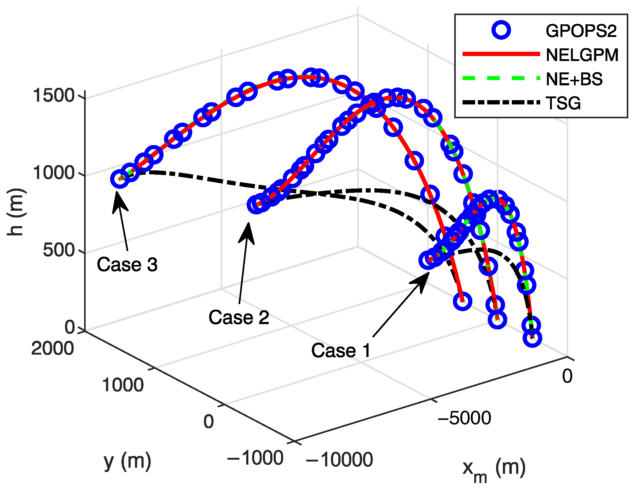
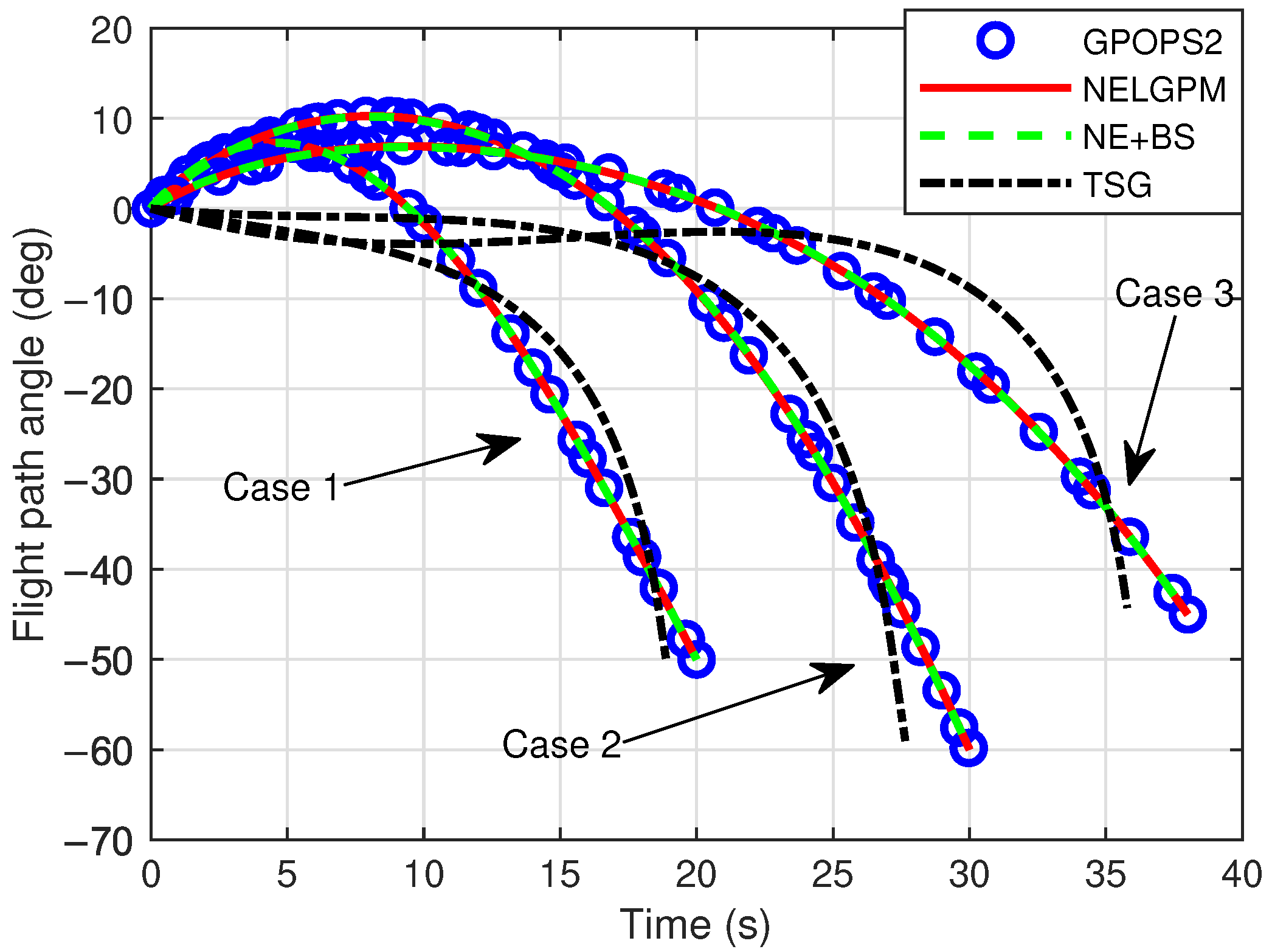
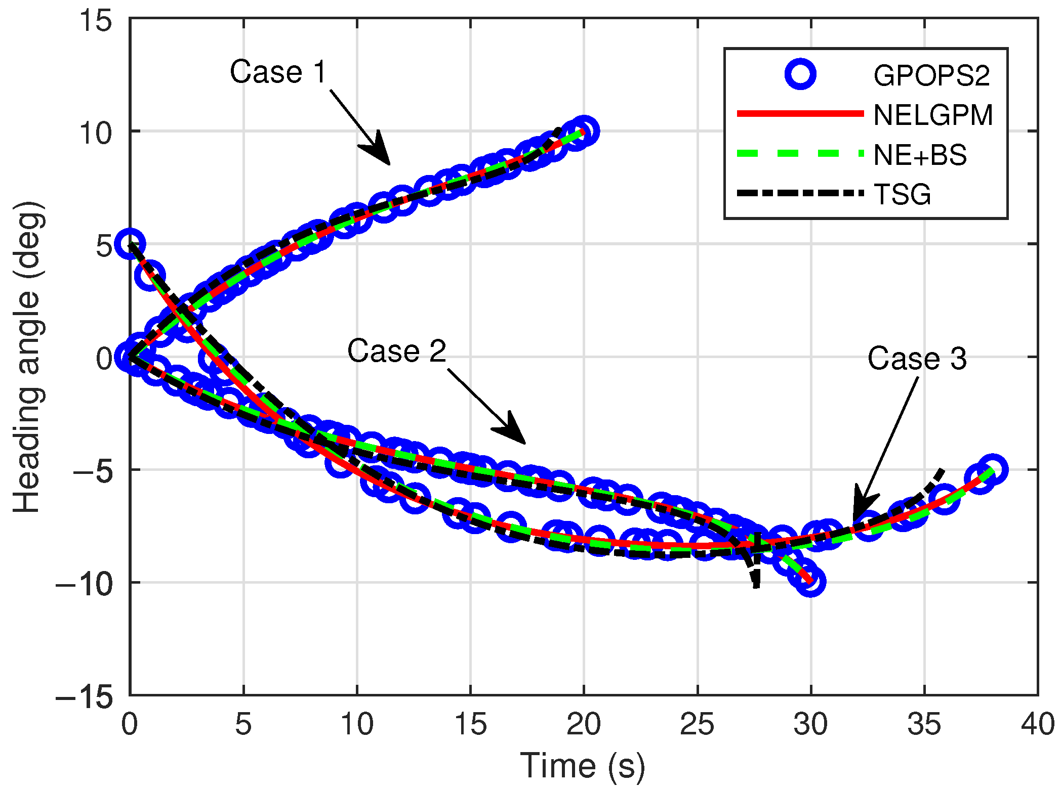
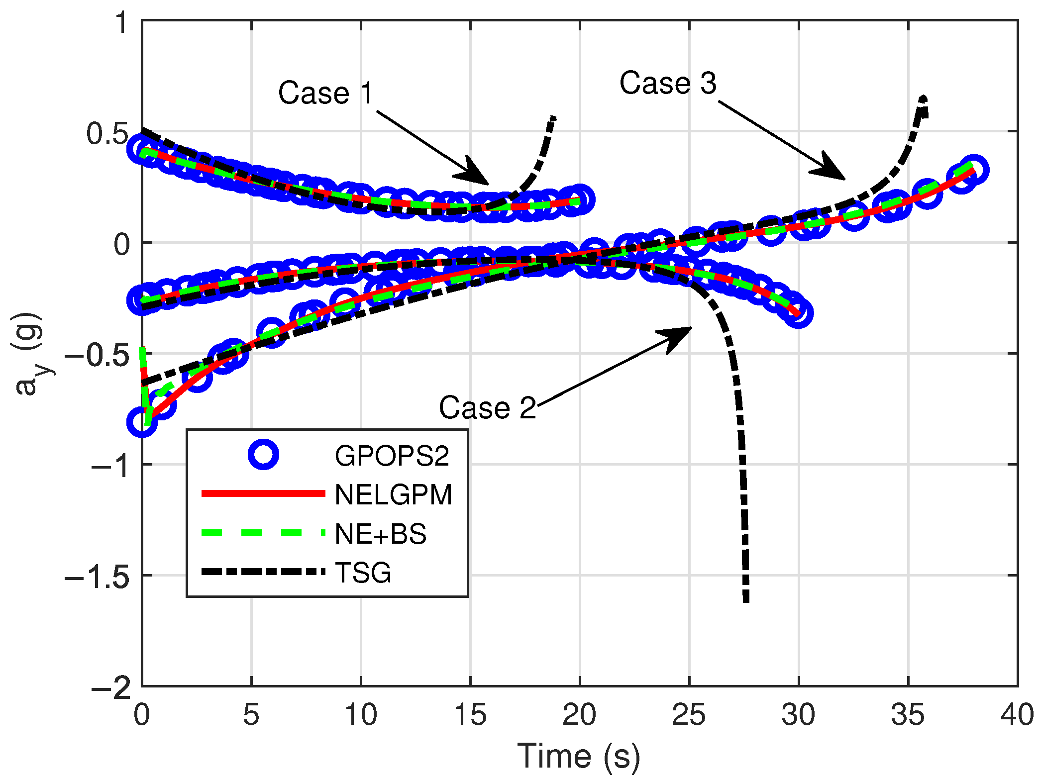
Firstly, comparative analyses were conducted between the guidance simulation results of the proposed method under three distinct scenarios and the offline optimized results from GPOPS-II with direct initial state deviations, as well as the simulated outcomes of NE + BS and TSG. The comparison results are illustrated in the following figures. The results show that this method can calculate the new optimal trajectory online with initial deviations and meet the given terminal constraints. Figure 2 shows the three-dimensional flight trajectories of the aircraft. Figure 3, Figure 4, and Figure 5 present the histories of the aircraft’s velocity, flight path angle, and heading angle, respectively. Moreover, the terminal constraints were all met in the three scenarios. Figure 6 and Figure 7 reveal the histories of the control variables of the aircraft, which exhibit smooth and continuous curves. This indicates that the proposed method is able to provide stable guidance commands. Table 5 shows the performance index for the simulations of different methods. It is evident that TSG produces considerable overload at the terminal stage and fails to control terminal velocity, resulting in the worst performance index. On the other hand, as can be seen from the figures, the proposed method provides the control curves that closely match those generated by the GPOPS-II. That means the proposed method achieves optimality. Furthermore, the results also indicate that the proposed method has great adaptability for cases where deviations in the initial and terminal conditions are highly different.

Figure 2. Comparison of flight trajectories.

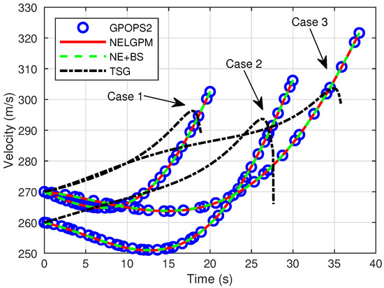
Figure 3. Comparison of velocity.

Figure 4. Comparison of flight path angle.

Figure 5. Comparison of heading angle.

Figure 6. Comparison of control $a_y$.

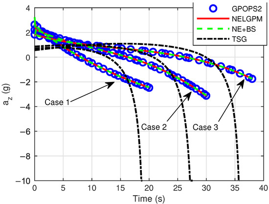
Figure 7. Comparison of control $a_z$.

Table 5. Comparison of performance indexes.

	Case 1	Case 2	Case 3
NELGPM	−32.5301	−46.3583	−51.6242
GPOPS-II	−32.5317	−46.3603	−51.6271
NE + BS	−32.5284	−46.3549	−51.6130
TSG	−19.2002	−6.0015	−28.6340

Subsequently, the computational efficiency and convergence speed of the proposed method were verified through simulation. The result clearly shows that only a few steps are needed to reach the optimal solution. The time consumption for the computational process consists of two parts. One part is to predict terminal errors, and the other part is to compute control updates. Table 6 illustrates the trajectory integration time and control update time per iteration for the proposed method across three scenarios. Due to the large number of integral nodes used, trajectory integration consumes most of the time. This takes about 0.02 s. The time consumption for the control update is only about 0.002 s. The reason is that this process only solves a set of linear algebraic equations. Consequently, the total time of a single iteration is only around 0.02 s, which shows that the proposed method is of high computational efficiency. Moreover, the backward sweep method requires the numerical integration of differential equations twice at each step, making its control update computation time dozens of times longer than the proposed method. With the implementation of more specialized computational algorithms and professional computing systems, the computational speed of the proposed method could be further enhanced, which has the potential for an online application.

Table 6. Time consumption of a single iteration.

Average Time Consumption (s)		Control Update	Trajectory Integration	Single Iteration
NELGPM	Case 1	0.0020	0.0151	0.0171
	Case 2	0.0020	0.0203	0.0223
	Case 3	0.0021	0.0244	0.0265
NE + BS	Case 1	0.0576	0.0149	0.0725
	Case 2	0.0627	0.0204	0.0831
	Case 3	0.0649	0.0242	0.0891

Table 7 illustrates the control update time and number of iterations using different numbers of nodes across three scenarios. For six nodes, the time consumption is about 0.0014 s, and the number of iterations is about 10. For 15 nodes, the time consumption is about 0.003 s, and the number of iterations is about 14. If there are too many nodes, the convergence speed will be reduced. Considering both the control update time and number of iterations, the optimal range for the number of nodes in the proposed method is between 8 and 12.

Table 7. Time consumption and iteration number for different numbers of points.

		Number of LG nodes
		6	8	10	12	15
Control update time (s)	Case 1	0.0014	0.0015	0.0020	0.0023	0.0027
	Case 2	0.0013	0.0015	0.0020	0.0023	0.0028
	Case 3	0.0013	0.0016	0.0021	0.0024	0.0029
Number of iterations	Case 1	10	9	9	9	15
	Case 2	10	9	9	9	10
	Case 3	10	9	9	9	12

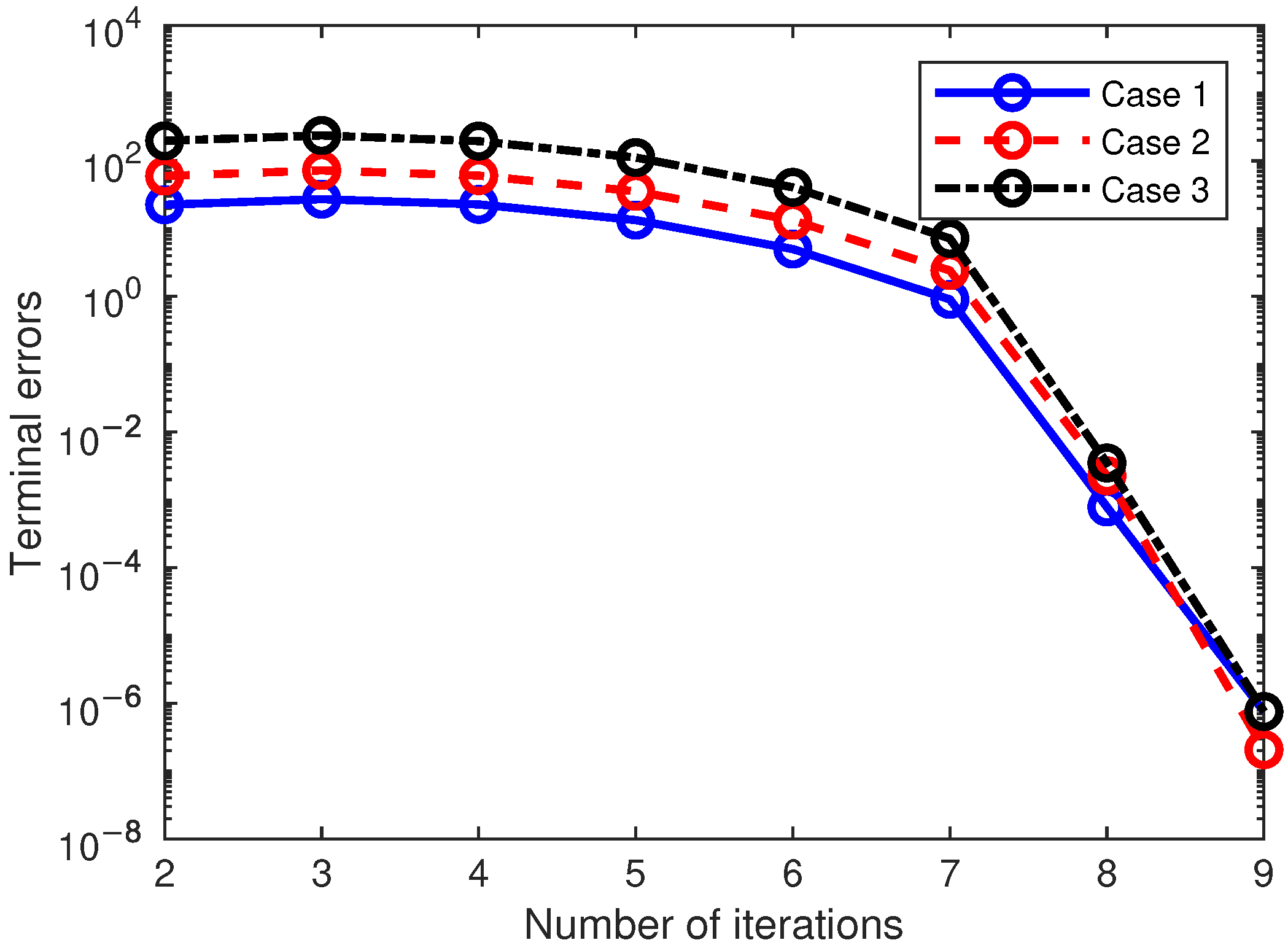
Next, the convergence process was analyzed through simulation results. The terminal error is a scalar value, which is the 2-norm of different terminal state errors including position and angle. Figure 8 shows the history of the terminal errors varying with the number of iterations. It can be observed that the convergence rate is notably slow during the initial iterations. As the neighboring optimal solutions gradually converge towards the global optimum, the iteration speed increases significantly. For all cases, it only takes nine iterations to reach the designated tolerance. Hence, the proposed method exhibits a remarkably high convergence speed.

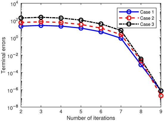
Figure 8. Variation in terminal error in three cases.

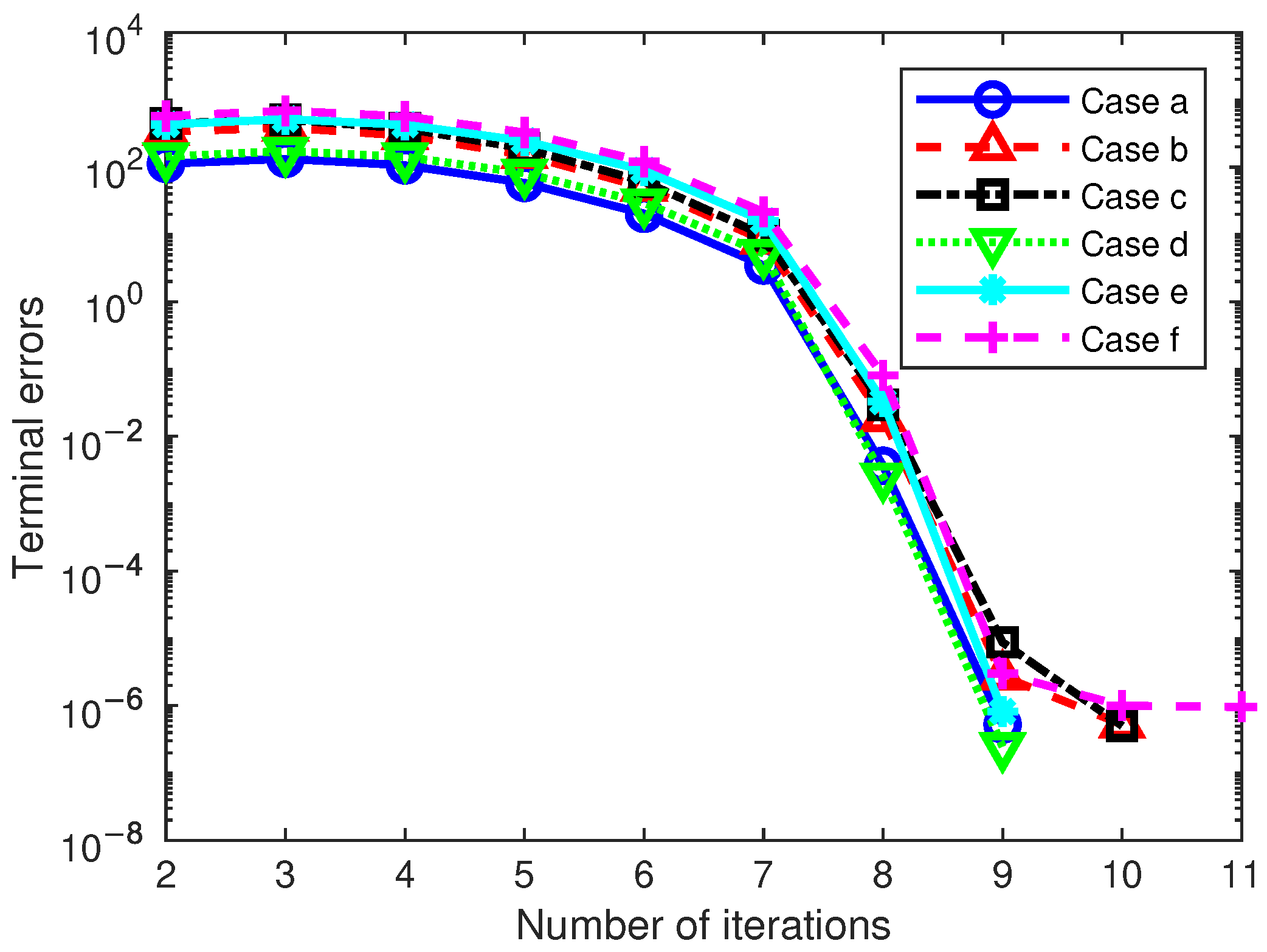
In addition, the magnitude of the initial deviations is also an important factor affecting the number of iterations of this method. In order to verify its impact on the number of iterations, the initial state deviations in Case 2 are changed to the six cases shown in Table 8. These include the deviations of the initial position and the initial angle. The simulation results of the number of iterations are shown in Figure 9. The results show that this method can converge with a certain number of iterations for a considerable initial state deviation. The larger the initial deviations, the more iterations are required. Therefore, we believe that when the initial state deviations are within the solvable range, the proposed method can obtain the optimal solution after the deviations through a certain number of iterations.

Table 8. Initial state deviations in Case 2.

	$\mathit{\delta }{\mathit{x}}_{\mathit{m}0}$ (m)	$\mathit{\delta }{\mathit{\psi }}_{\mathit{V}0}$ (deg)
Case a	500	0
Case b	1500	0
Case c	2000	0
Case d	0	−5
Case e	0	−15
Case f	0	−20

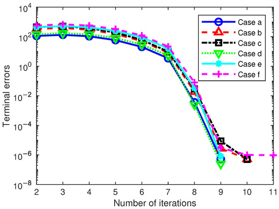
Figure 9. Initial state deviations in Case 2.

4.4. Monte Carlo Simulation

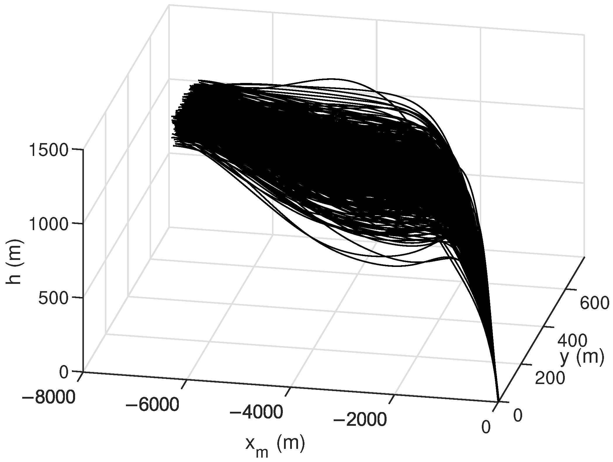
Finally, Monte Carlo simulations were carried out to verify the robustness of the proposed method. Simulation conditions were the same as those in Case 2. Uncertainties in atmospheric density and aerodynamic coefficients in actual aircraft flight operations were considered in the simulation. These uncertainties involved initial state variables, atmospheric density, and aerodynamic coefficients. The deviations in initial state variables followed both uniform and Gaussian distributions, while deviations in atmospheric density and aerodynamic coefficients followed Gaussian distributions, with specific parameter distributions outlined in Table 9. The results of 500 Monte Carlo simulations are shown in Figure 10, Figure 11 and Figure 12. The terminal errors are summarized in Table 10.

Table 9. Dispersion of parameters.

Parameters	Distribution	3$\mathit{\sigma }$ or Max/Min
$\delta x_{m0}$ (m)	Uniform	±100
$\delta y_0$ (m)	Uniform	±100
$\delta h_0$ (m)	Uniform	±100
$\delta V_0$ (m/s)	Gaussian	±5
$\delta {\gamma }_0$ (deg)	Gaussian	±5
$\delta {\psi }_{V0}$ (deg)	Gaussian	±5
$\rho$ (kg/m3)	Gaus sian	±10%
$C_L$	Gaussian	±10%
$C_D$	Gaussian	±10%

Figure 10. Monte Carlo simulation results of flight trajectories.

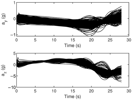
Figure 11. Monte Carlo simulation results of control variables.

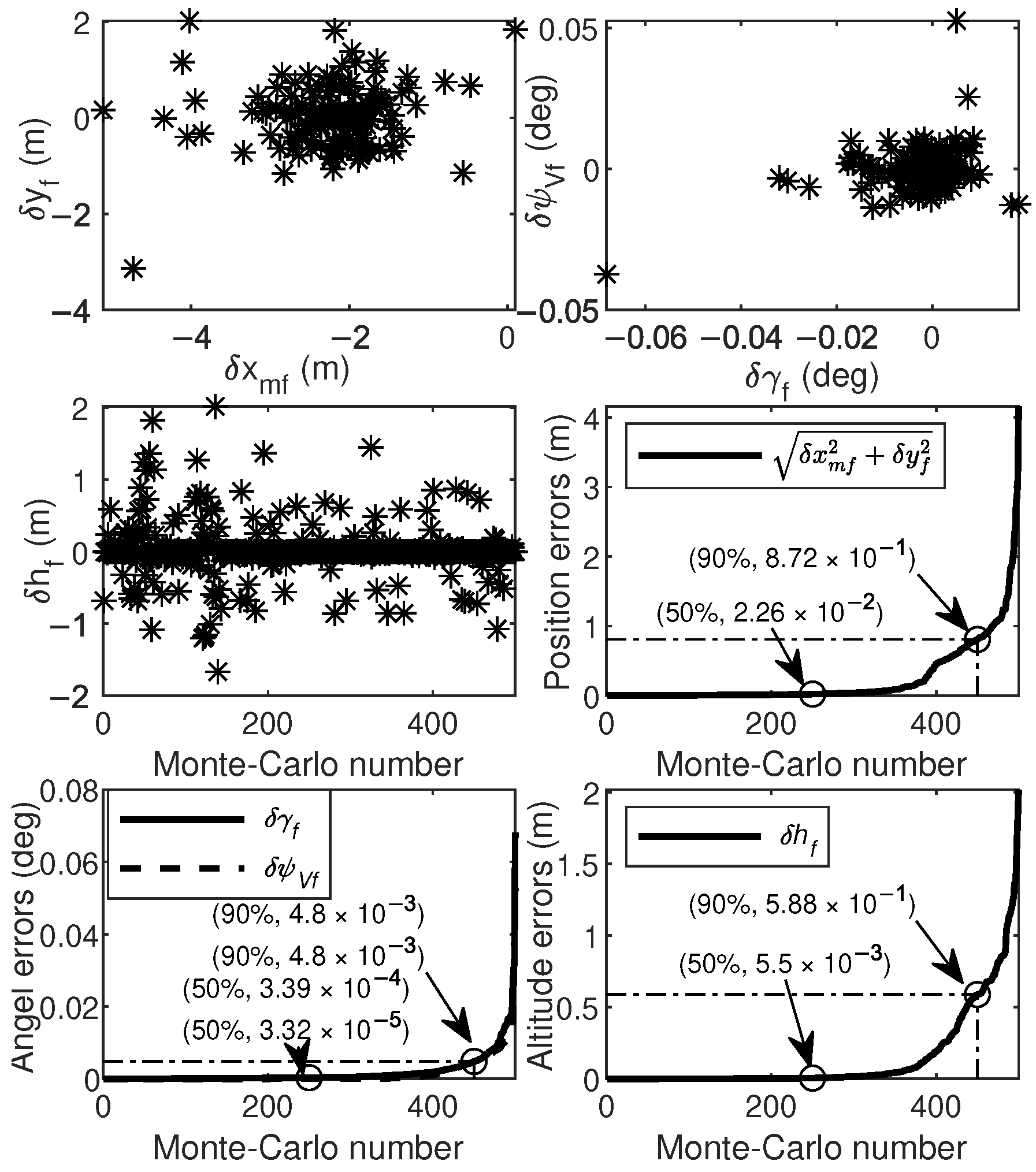
Figure 12. Monte Carlo simulation results of terminal errors.

Table 10. Mean and variance of terminal errors.

Termial Errors	Mean	Variance
$\delta x_{mf}$ (m)	−$6.83\times {10}^{-2}$	$1.61\times {10}^{-1}$
$\delta y_f$ (m)	$1.27\times {10}^{-2}$	$1.16\times {10}^{-1}$
$\delta h_f$ (m)	$1.10\times {10}^{-2}$	$1.12\times {10}^{-1}$
$\delta {\gamma }_f$ (deg)	$-6.35\times {10}^{-4}$	$4.45\times {10}^{-7}$
$\delta {\psi }_{Vf}$ (deg)	$3.57\times {10}^{-5}$	$3.00\times {10}^{-7}$

Figure 10 shows the flight trajectory from the Monte Carlo simulations. It is evident that the proposed method performs well in guiding the aircraft towards the specified target, even under various random perturbation conditions. Figure 11 shows the control histories from the Monte Carlo simulation results. Notably, the proposed method provides stable and smooth control commands for all cases, which is beneficial for practical applications. Figure 12 shows the terminal errors from Monte Carlo simulations. It is evident that the maximum terminal position error is within 5 m, and the maximum terminal angle error is within 0.1 degrees.

Table 10 shows the means and variances of these errors. The mean terminal position errors are within 0.01 m. The mean terminal angle errors are within $1\times {10}^{-4}$ degrees. The variances of position are around 0.1. The variances of angle are around $1\times {10}^{-7}$. Consequently, the proposed method demonstrates excellent performance and robustness even in highly uncertain environments.

5. Conclusions

This paper proposes a neighboring extremal linear Gauss pseudospectral method for online solving the nonlinear OCP with an arbitrary performance index. This method takes advantage of Gauss pseudospectral collocation and the neighboring extremal method, converting the solution of OCP with deviations into an iterative solution of linear algebraic equations. Furthermore, the control correction can be derived in an analytical manner. Therefore, it can provide the control updates coming close to the optimal control with high computational efficiency and accuracy. This method is applied to a guidance example for air-to-ground aircraft. Some nominal simulations, comparisons, and Monte Carlo simulations were carried out to test the performance of the method. The results show that, for different scenarios, it only takes a fraction of one second to get the solution satisfying the tolerance, which is consistent with the optimal solution generated by GPOPS-II. The proposed method appears to have good adaptability, strong robustness, high computational accuracy, and efficiency. Consequently, it fully meets the requirements of online application for closed-loop guidance.

References

- Cardoso, D.N.; Esteban, S.; Raffo, G.V. A robust optimal control approach in the weighted Sobolev space for underactuated mechanical systems. Automatica 2021, 125, 109474. [Google Scholar] [CrossRef]
- Zhao, S.; Chen, W.; Yang, L. Optimal guidance law with impact-angle constraint and acceleration limit for exo-atmospheric interception. Aerospace 2021, 8, 358. [Google Scholar] [CrossRef]
- Nolasco, E.; Vassiliadis, V.S.; Kähm, W.; Adloor, S.D.; Al Ismaili, R.; Conejeros, R.; Espaas, T.; Gangadharan, N.; Mappas, V.; Scott, F. Optimal control in chemical engineering: Past, present and future. Comput. Chem. Eng. 2021, 155, 107528. [Google Scholar] [CrossRef]
- Yang, C.; Xia, Y. Interval uncertainty-oriented optimal control method for spacecraft attitude control. IEEE Trans. Aerosp. Electron. Syst. 2023, 59, 5460–5471. [Google Scholar] [CrossRef]
- Ozaki, N.; Campagnola, S.; Funase, R. Tube stochastic optimal control for nonlinear constrained trajectory optimization problems. J. Guid. Control Dyn. 2020, 43, 645–655. [Google Scholar] [CrossRef]
- Morante, D.; Sanjurjo Rivo, M.; Soler, M. A survey on low-thrust trajectory optimization approaches. Aerospace 2021, 8, 88. [Google Scholar] [CrossRef]
- Huntington, G.T.; Rao, A.V. Optimal reconfiguration of spacecraft formations using the Gauss pseudospectral method. J. Guid. Control Dyn. 2008, 31, 689–698. [Google Scholar] [CrossRef]
- Garg, D.; Patterson, M.A.; Francolin, C.; Darby, C.L.; Huntington, G.T.; Hager, W.W.; Rao, A.V. Direct trajectory optimization and costate estimation of finite-horizon and infinite-horizon optimal control problems using a Radau pseudospectral method. Comput. Optim. Appl. 2011, 49, 335–358. [Google Scholar] [CrossRef]
- Tian, B.; Zong, Q. Optimal guidance for reentry vehicles based on indirect Legendre pseudospectral method. Acta Astronaut. 2011, 68, 1176–1184. [Google Scholar] [CrossRef]
- Guo, X.; Zhu, M. Direct trajectory optimization based on a mapped Chebyshev pseudospectral method. Chin. J. Aeronaut. 2013, 26, 401–412. [Google Scholar] [CrossRef]
- Fahroo, F.; Ross, I.M. Pseudospectral methods for infinite-horizon nonlinear optimal control problems. J. Guid. Control Dyn. 2008, 31, 927–936. [Google Scholar] [CrossRef]
- Vlassenbroeck, J. A Chebyshev polynomial method for optimal control with state constraints. Automatica 1988, 24, 499–506. [Google Scholar] [CrossRef]
- Vlassenbroeck, J.; Van Dooren, R. A Chebyshev technique for solving nonlinear optimal control problems. IEEE Trans. Autom. Control 1988, 33, 333–340. [Google Scholar] [CrossRef]
- Elnagar, G.; Kazemi, M.A.; Razzaghi, M. The pseudospectral Legendre method for discretizing optimal control problems. IEEE Trans. Autom. Control 1995, 40, 1793–1796. [Google Scholar] [CrossRef]
- Elnagar, G.N.; Kazemi, M.A. Pseudospectral Chebyshev optimal control of constrained nonlinear dynamical systems. Comput. Optim. Appl. 1998, 11, 195–217. [Google Scholar] [CrossRef]
- Fahroo, F.; Ross, I.M. Direct trajectory optimization by a Chebyshev pseudospectral method. J. Guid. Control Dyn. 2002, 25, 160–166. [Google Scholar] [CrossRef]
- Rao, A.; Clarke, K. Performance optimization of a maneuvering re-entry vehicle using a legendre pseudospectral method. In Proceedings of the AIAA Atmospheric Flight Mechanics Conference And Exhibit, Monterey, CA, USA, 5–8 August 2002; p. 4885. [Google Scholar]
- Benson, D. A Gauss Pseudospectral Transcription for Optimal Control. Ph.D. Thesis, Massachusetts Institute of Technology, Cambridge, MA, USA, 2005. [Google Scholar]
- Fahroo, F.; Ross, I.M. Costate Estimation by a Legendre Pseudospectral Method. J. Guid. Control Dyn. 2001, 24, 270–277. [Google Scholar] [CrossRef]
- Darby, C.L.; Garg, D.; Rao, A.V. Costate Estimation using Multiple-Interval Pseudospectral Methods. J. Spacecr. Rockets 2011, 48, 856–866. [Google Scholar] [CrossRef]
- Chen, W.; Du, W.; Hager, W.W.; Yang, L. Bounds for integration matrices that arise in Gauss and Radau collocation. Comput. Optim. Appl. 2019, 74, 259–273. [Google Scholar] [CrossRef]
- Huntington, G.; Benson, D.; Rao, A. A Comparison of Accuracy and Computational Efficiency of Three Pseudospectral Methods. In Proceedings of the AIAA Guidance, Navigation and Control Conference and Exhibit, Hilton Head, SC, USA, 20–23 August 2007. [Google Scholar] [CrossRef]
- Gong, Q.; Ross, I.M.; Fahroo, F. Costate Computation by a Chebyshev Pseudospectral Method. J. Guid. Control Dyn. 2010, 33, 623–628. [Google Scholar] [CrossRef]
- Yang, S.; Cui, T.; Hao, X.; Yu, D. Trajectory optimization for a ramjet-powered vehicle in ascent phase via the Gauss pseudospectral method. Aerosp. Sci. Technol. 2017, 67, 88–95. [Google Scholar] [CrossRef]
- Garrido, J.V.; Sagliano, M. Ascent and descent guidance of multistage rockets via pseudospectral methods. In Proceedings of the AIAA SciTech 2021 Forum, Virtual, 11–21 January 2021; p. 0859. [Google Scholar]
- Padhi, R.; Kothari, M. Model predictive static programming: A computationally efficient technique for suboptimal control design. Int. J. Innov. Comput. Inf. Control 2009, 5, 399–411. [Google Scholar]
- Varma, S.A.; Parwana, H.; Kothari, M. A Pitch Controlled Impact-Angle-Constrained Guidance Law for Surface-to-Surface Missiles. In Proceedings of the AIAA Guidance, Navigation, and Control Conference, San Diego, CA, USA, 4–8 January 2016; p. 2114. [Google Scholar]
- Mondal, S.; Padhi, R. Angle-constrained terminal guidance using quasi-spectral model predictive static programming. J. Guid. Control Dyn. 2018, 41, 783–791. [Google Scholar] [CrossRef]
- Yang, L.; Zhou, H.; Chen, W. Application of linear gauss pseudospectral method in model predictive control—ScienceDirect. Acta Astronaut. 2014, 96, 175–187. [Google Scholar] [CrossRef]
- Yang, L.; Liu, X.; Chen, W.; Zhou, H. Autonomous entry guidance using Linear Pseudospectral Model Predictive Control. Aerosp. Sci. Technol. 2018, 80, 38–55. [Google Scholar] [CrossRef]
- Li, Y.; Chen, W.; Yang, L. Multistage linear gauss pseudospectral method for piecewise continuous nonlinear optimal control problems. IEEE Trans. Aerosp. Electron. Syst. 2021, 57, 2298–2310. [Google Scholar] [CrossRef]
- Li, Y.; Chen, W.; Yang, L. Linear Pseudospectral Method with Chebyshev Collocation for Optimal Control Problems with Unspecified Terminal Time. Aerospace 2022, 9, 458. [Google Scholar] [CrossRef]
- Zhou, C.; He, L.; Yan, X.; Meng, F.; Li, C. Active-set pseudospectral model predictive static programming for midcourse guidance. Aerosp. Sci. Technol. 2023, 134, 108137. [Google Scholar] [CrossRef]
- Tang, G.; Jiang, F.; Li, J. Fuel-optimal low-thrust trajectory optimization using indirect method and successive convex programming. IEEE Trans. Aerosp. Electron. Syst. 2018, 54, 2053–2066. [Google Scholar] [CrossRef]
- Wang, Z.; Lu, Y. Improved sequential convex programming algorithms for entry trajectory optimization. J. Spacecr. Rockets 2020, 57, 1373–1386. [Google Scholar] [CrossRef]
- Sagliano, M. Pseudospectral convex optimization for powered descent and landing. J. Guid. Control Dyn. 2018, 41, 320–334. [Google Scholar] [CrossRef]
- Li, Y.; Chen, W.; Yang, L. Successive Chebyshev pseudospectral convex optimization method for nonlinear optimal control problems. Int. J. Robust Nonlinear Control 2022, 32, 326–343. [Google Scholar] [CrossRef]
- Breakwell, J.V.; Speyer, J.L.; Bryson, A.E. Optimization and control of nonlinear systems using the second variation. J. Soc. Ind. Appl. Math. Ser. Control 1963, 1, 193–223. [Google Scholar] [CrossRef]
- Bryson, A.E.; Ho, Y.C. Applied Optimal Control; Blaisdell Publishing Company: Waltham, MA, USA, 1969. [Google Scholar]
- Hull, D.G. Sufficient conditions for a minimum of the free-final-time optimal control problem. J. Optim. Theory Appl. 1991, 68, 275–287. [Google Scholar] [CrossRef]
- Ghaemi, R.; Jing, S.; Kolmanovsky, I.V. Neighboring Extremal Solution for Nonlinear Discrete-Time Optimal Control Problems With State Inequality Constraints. IEEE Trans. Autom. Control 2009, 54, 2674–2679. [Google Scholar] [CrossRef]
- Chen, Z.; Tang, S. Neighboring optimal control for open-time multiburn orbital transfers. Aerosp. Sci. Technol. 2018, 74, 37–45. [Google Scholar] [CrossRef]
- Feng, Y.; Chen, W.; Yang, L.; Wei, D. Optimal Terrain Following Trajectory Regeneration Using Linear Gauss Pseudo-Spectral Method. In Proceedings of the 2019 IEEE International Conference on Unmanned Systems (ICUS), Beijing, China, 17–19 October 2019; pp. 205–211. [Google Scholar]
- Bagherzadeh, S.; Karimpour, H.; Keshmiri, M. Neighboring extremal nonlinear model predictive control of a rigid body on SO(3). Robotica 2023, 41, 1313–1334. [Google Scholar] [CrossRef]
- Rai, A.; Mou, S.; Anderson, B.D. Closed-Loop Neighboring Extremal Optimal Control Using HJ Equation. In Proceedings of the 2023 62nd IEEE Conference on Decision and Control (CDC), Singapore, 13–15 December 2023; pp. 3270–3275. [Google Scholar]
- Vahidi-Moghaddam, A.; Zhang, K.; Li, Z.; Wang, Y. Data-Enabled Neighboring Extremal Optimal Control: A Computationally Efficient DeePC. In Proceedings of the 2023 62nd IEEE Conference on Decision and Control (CDC), Singapore, 13–15 December 2023; pp. 4778–4783. [Google Scholar]
- Ohlmeyer, E.J.; Phillips, C.A. Generalized vector explicit guidance. J. Guid. Control Dyn. 2006, 29, 261–268. [Google Scholar] [CrossRef]
- Patterson, M.A.; Rao, A.V. GPOPS-II: A MATLAB software for solving multiple-phase optimal control problems using hp-adaptive Gaussian quadrature collocation methods and sparse nonlinear programming. ACM Trans. Math. Software 2014, 41, 1–37. [Google Scholar] [CrossRef]
- Hodgson, J.; Lee, D. Terminal guidance using a Doppler beam sharpening radar. In Proceedings of the AIAA Guidance, Navigation, and Control Conference and Exhibit, Austin, TX, USA, 11–14 August 2003; p. 5796. [Google Scholar]
Disclaimer/Publisher’s Note: The statements, opinions and data contained in all publications are solely those of the individual author(s) and contributor(s) and not of MDPI and/or the editor(s). MDPI and/or the editor(s) disclaim responsibility for any injury to people or property resulting from any ideas, methods, instructions or products referred to in the content. |
© 2025 by the authors. Licensee MDPI, Basel, Switzerland. This article is an open access article distributed under the terms and conditions of the Creative Commons Attribution (CC BY) license (https://creativecommons.org/licenses/by/4.0/).