Dynamics and Staged Deployment Strategy for a Spinning Tethered Satellite System

Abstract

This paper investigates flexible multibody dynamic modeling and a staged deployment strategy for large-scale spinning tethered satellite systems, targeting deployment instability, inefficiencies, and tension-induced fracture risks. A nonlinear flexible multibody model is constructed using the absolute nodal coordinate formulation within an arbitrary Lagrangian–Eulerian framework, enabling accurate large-deformation modeling of the tether with geometric nonlinearity. This model surpasses traditional massless/rigid rod models by integrating tether mass distribution, flexible dynamics, and satellite attitude dynamics. A two-stage deployment strategy is proposed based on tether safe tension thresholds. Stage 1 optimizes deployment velocity to eliminate libration angles, ensuring stability while maintaining deployment efficiency. Stage 2 employs dynamic angular velocity tracking and torque compensation to reduce tether tension, prioritizing deployment safety. Numerical simulations validate the model’s accuracy and the strategy’s effectiveness, showing significant tension reduction compared to the single-stage strategy and suppressing libration angle oscillations within ±0.5°. The impact of space environmental forces on deployment stability across different orientations is analyzed, highlighting the necessity of force compensation for parallel-to-ground configurations. This research integrates dynamics and control, providing a practical solution for safe and efficient deployment of the spinning tethered satellite system.

1. Introduction

In recent years, as a remarkable space technology, the tethered satellite system has exhibited broad prospects for applications in fields such as the astrophysical observation, earth remote sensing, and space science research [1,2,3]. The spinning tethered satellite system (STSS) is composed of a central spacecraft and multiple sub-satellites connected by tethers, which can transmit force and energy. By adjusting the tether length, the formation and scale can be flexibly adjusted. Meanwhile, the centrifugal force generated by the spin of the central spacecraft allows the system to maintain structural dynamic stability [4].

The tether of the STSS typically ranges in length from tens to hundreds of meters. The process of deployment and maintaining the configuration of the ultra-long flexible tethers may yield large deformations and complex vibrations. Researchers have proposed various dynamic models, including the dumbbell, lumped mass, and continuum models, to investigate the dynamic behaviors of tethered satellite systems [5,6]. The dumbbell model, which is the simplest and most commonly used, considers the tether as a straight rigid rod without bending deformation. Misra et al. [7] analyzed the dynamic behaviors of tether satellite systems using the dumbbell model, assuming rigid, massless, and constant-length tethers. Luo et al. [8] considered the electrodynamic tether as a rigid rod, neglecting tether length variation and bending deformation. The lumped mass model divides the tether into a series of mass points and springs, which further improves the model accuracy of the flexible tether [9,10,11]. Moreover, the accuracy and computational efficiency of the continuum model approach, particularly the absolute nodal coordinate formulation (ANCF), has made significant improvements [12,13,14]. Shabana [15] proposed the ANCF approach by using the absolute positions and gradients of nodes to describe the configurations of flexible bodies. Shan et al. [16] applied the ANCF method to model a tether net system for debris removal in space, and the results showed that the ANCF model outperformed the mass-spring model in describing system dynamics. Tang et al. [17] proposed the ANCF-arbitrary Lagrange–Eulerian (ALE) model, which accurately captures dynamic characteristics during the deployment and retrieval of the tether. This variable-length cable element has been widely applied for the dynamic analysis of tethered satellite systems. Zhang et al. [18] established the dynamic model of a tethered satellite system using the ANCF method in an ALE framework, considering the gravity gradient and Coriolis force in space orbit environments. The study identified that, when the deployment strategy is unreasonable, the tethered satellite may experience a rebound phenomenon, leading to decreased system stability. Wang et al. [19] applied the ANCF method to derive a flexible dynamic model for the electric sail. The numerical results showed that the tether rotates in a spin plane accompanied with large flexible deformation, and there exists an out-of-plane angle between the tether and the spin plane due to solar winds. Sun et al. [20,21] used the ANCF and the natural coordinate formulation (NCF) to precisely characterize the large deformations of flexible tethers and overall motions of rigid satellites in their investigation of tethered satellite formations. It was found that increasing the sub-satellite mass and reducing spinning speed could enhance formations stability. In summary, while researchers have explored various dynamic models for tethered satellite systems, the existing research is still dominated by rigid models or lumped mass models. The ANCF approach is mainly used for the analysis of system dynamics phenomenon and is rarely used in deployment control analysis.

As a spin-stabilized rotating deployable structure, the STSS is similar to electric sails and long thin wire antennas and is typically designed as a collection of slender flexible bodies with end masses [22,23]. Researchers have attempted to address the deployment challenges associated with spin-stabilized structures. Early research by Tragesser and Gorjidooz [24] thoroughly explored the spin-up and deployment control of a single tether sling system, developing open-loop control laws for both power-unlimited and power-constrained scenarios. Their simulations at 0.05 rad/s indicated that deploying a tether to 20 km resulted in a peak tension of 76 kN, highlighting the extreme tension risks involved in the deployment of large-scale STSSs. Huang et al. [25] investigated the configuration of a rotating hub–spoke formation system consisting of a rigid hub and two tethers, solving the optimal deployment and retrieval control problems using the Gauss pseudospectral method to obtain the optimal trajectory. Zhai et al. [26] studied the deployment strategy of a planar multi-tether satellite formation by treating the tether as a rigid massless rod, considering the influence of gravity gradient and suppressing the deployment vibration of the system by planning the spin rate and the tether deployment velocity. Additionally, Fulton et al. [27] examined two deployment schemes for electric sails, namely, radial and tangential deployment, deriving the tether deployment strategy under the constant rotation speed condition of the system while considering tether mass but overlooking its influence on tether tension. Furthermore, Liu et al. [28] proposed a tension control strategy based on a nonlinear sliding mode controller to stably deploy the underactuated hub–spoke tethered satellite formation using controlled tether deployment speed. Su et al. [29] treated the tethers of the satellite formation as linear elastic bodies with uniformly distributed mass, planning the tether deployment velocity and spin rate of the central spacecraft under constant velocity or acceleration conditions. Considering that the flexibility of structures is essential when investigating spin-stabilized rotating deployable structures, some studies, such as the study by Li et al. [30], modeled a solar wind sail using the finite element method, considering the flexible dynamics of conductive tethers but ignoring the significant tension owing to the mass of the large-scale tether structure during deployment. The deployment of Radiation Belt Storm Probe (RBSP) antenna, led by NASA, was periodically paused to avoid the divergence of the libration angle until the maximum length was reached, but this multi-stage deployment method takes a long time to deploy the antenna to 50 m [31]. Overall, these studies provide valuable references for the deployment strategies related to spin-stabilized tethered systems. However, many of the deployment control analysis employed in these studies made significant simplifications, such as ignoring the flexibility and mass of tethers in the dynamic model. Furthermore, these studies do not address the potential issue of extreme tether tension that may arise at large scales and high rotation speeds.

The aforementioned pieces of research have explored various dynamic models and deployment strategies for the STSS. However, previous research usually overlooked the flexibility and mass of the tethers in the spinning deployment control analysis, and the dynamic behaviors of the rigid model and the flexible model were not fully comparatively analyzed. Moreover, the tether fracture issue caused by extreme tether tension, which has a chance to occur in large-scale STSSs, was usually neglected in the research of deployment strategies. To better address the above issues in the deployment of the STSS, this paper is organized as follows. An accurate dynamic model of the flexible tether is established using ANCF within an ALE framework, and the flexible multibody dynamic equations of STSSs are presented in Section 2. Section 3 presents a staged deployment strategy that considers the maximum tension of the tether during deployment, ensuring efficient and safe deployment for large-scale STSSs. In Section 4, the numerical simulation shows the superiority of the dynamic model in this paper compared with the traditional rigid model and demonstrates the effectiveness of the proposed staged deployment strategy. Section 5 concludes this paper.

2. Dynamic Modeling of the STSS

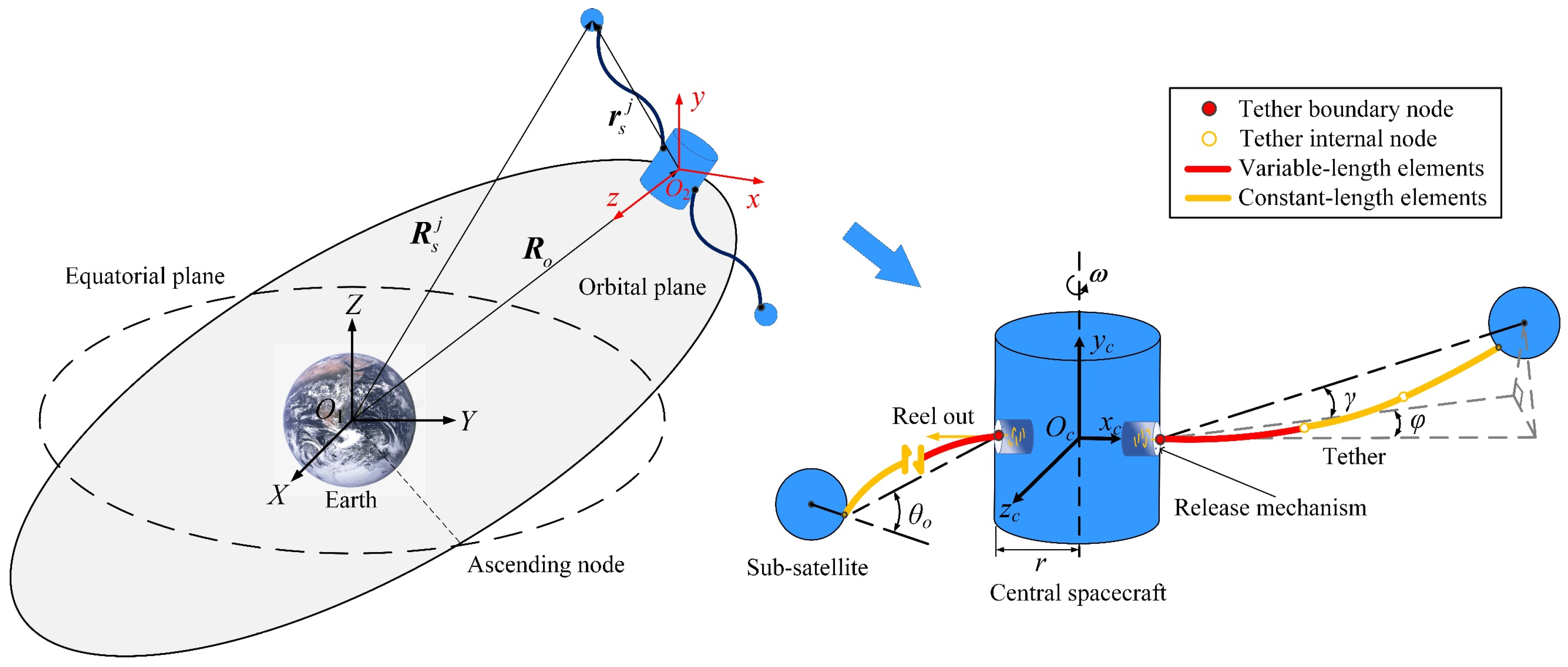
2.1. System Description

As shown in Figure 1, the STSS operating in Earth’s orbit is composed of a central spacecraft and multiple sub-satellites interconnected by tethers. Ideally, the sub-satellites are symmetrically positioned around the central spacecraft. The tether release mechanisms are symmetrically positioned along the periphery of the central spacecraft. The central spacecraft provides rotational torque for the spinning deployment process. The central spacecraft and sub-satellites are regarded as rigid bodies, while the tensile and bending deformations and the mass of the tether system are considered.

To describe the motion and deformation of the STSS, three coordinate frames are defined, as illustrated in Figure 1: the geocentric inertial coordinate frame $O_{1}XYZ$, the orbital coordinate frame $O_{2}xyz$, and the body-fixed coordinate frame $O_c{x}_c{y}_c{z}_c$ of the central spacecraft. In the geocentric inertial coordinate frame $O_{1}XYZ$, the $O_{1}Z$ axis aligns with the Earth’s rotational axis, while the $O_{1}X$ and $O_{1}Y$ axes lie within the equatorial plane. In the orbital coordinate frame $O_{2}xyz$, the $O_{2}x$ axis points in the flight direction, the $O_{2}z$ axis is directed toward the Earth’s core, and the $O_{2}y$ can be determined by the right-hand rule. The origin of body-fixed coordinate frame $O_c{x}_c{y}_c{z}_c$ is located at the center of the central spacecraft, and the $O_c{y}_c$ axis aligns with the spin axis. The key parameters $\phi$, $\gamma$, and ${\theta }_o$, characterizing the stability of the STSS, will be elaborated in the following sections.

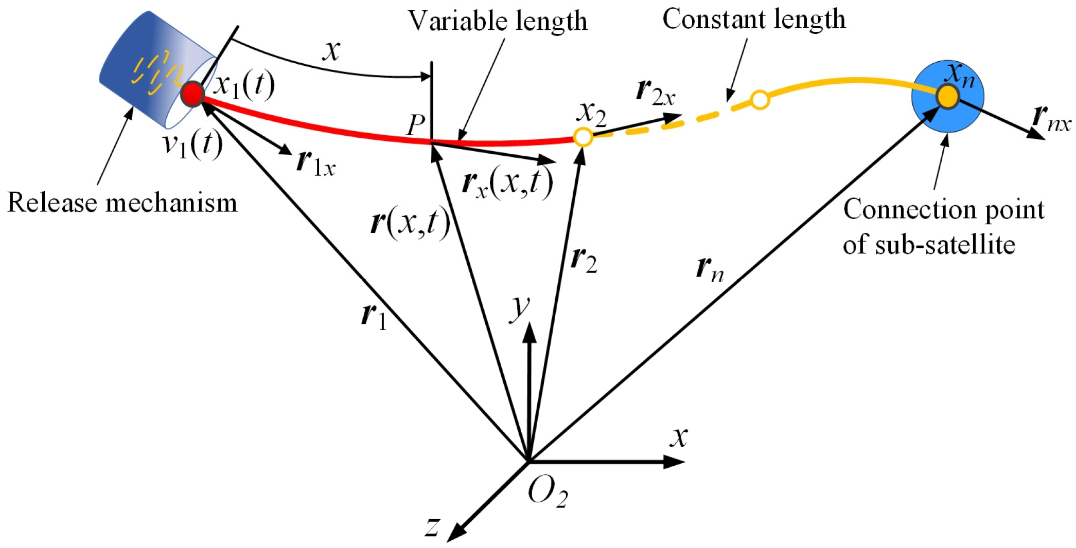
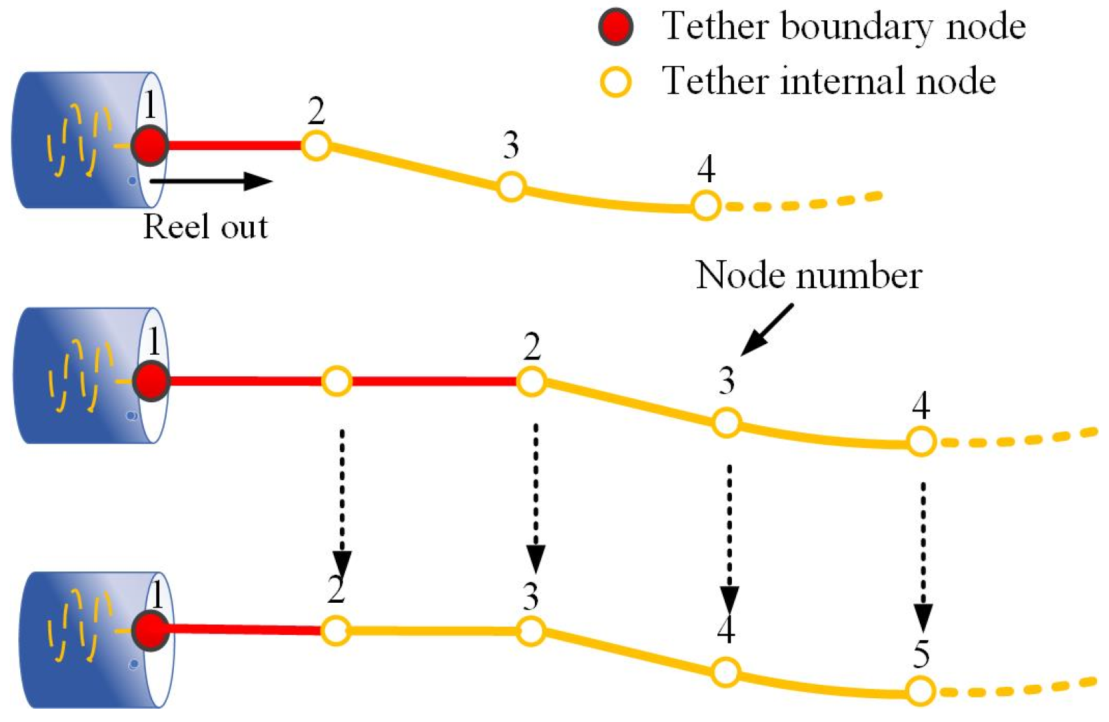
2.2. Dynamic Modeling of the Flexible Variable-Length Tether Element

Traditional modeling methods often encounter challenges, including limited model accuracy and low computational efficiency, when addressing the nonlinear dynamic behavior of flexible bodies with strong rigid-flexible couplings. When it comes to the flexible space tether system, the large deformation has an effect on the efficiency, safety, and stability of the tether deployment process. Therefore, in this article, the ANCF cable element in the framework of the ALE method [17] is employed to overcome these issues. This modeling approach makes use of a reduced number of elements to describe the slender space tether with large flexibility and a superimposed mass moving at one end. Considering the large slenderness ratio, only axial and bending deformations are incorporated into the dynamic prediction of the space tether during deployment and position-control stages.

As depicted in Figure 2, a variable-length element with mass moving at one end contains an Eulerian node corresponding to the moving boundary $x_1(t)$ and a Lagrangian node at the fixed boundary $x_2$. In terms of practical application, the deployment and retrieval of the tether are regulated by the release mechanism installed on the central spacecraft. Under this circumstance, a moving Eulerian node replaces one of the Lagrangian node in the original ANCF element, and the resulting element can be classified as the ANCF-ALE element. The moving Eulerian node no longer corresponds to a certain material coordinate $x_i$. Instead, the Eulerian node represents the kinematic states of masses that constantly flow through the moving boundary. Therefore, the material coordinate corresponding to the left moving boundary of the tether element is time-dependent and denoted as follows:

$${\dot{x}}_1(t)=-v_1(t)$$

(1)

Based on Equation (1), the tether system can control the element length by adjusting the value of $v_1(t)$. For instance, when $v_1(t)>0$, the Eulerian node moves away from the Lagrange node and the element length increases. When $v_1(t)<0$, the Eulerian node moves towards the Lagrange node and the element length decreases. In the particular case of $v_1(t)=0$, the variable-length ANCF-ALE tether element degenerates to a conventional constant-length element. In this article, $v_1(t)$ represents the deployment velocity of the tether.

The kinematic description of the variable-length tether element relies on the time-varying displacement field. As shown in Figure 2, to ensure $C^1$ continuity of the tether element, the global position vector $\mathit{r}\left(x,t\right)\in {ℝ}^3$ of any material point $P$ on the tether element is defined using cubic Hermite interpolation about the material coordinate $x$ as follows:

$$\mathit{r}\left(x,t\right)=\left[\begin{array}{c}{r}_1\\ r_2\\ r_3\end{array}\right]=\left[\begin{array}{c}{a}_0(t)+a_1(t)x+a_2(t)x^2+a_3(t)x^3\\ b_0(t)+b_1(t)x+b_2(t)x^2+b_3(t)x^3\\ c_0(t)+c_1(t)x+c_2(t)x^2+c_3(t)x^3\end{array}\right]$$

(2)

where the coefficients $a_k$, $b_k$, and $c_k$ ($k=1, 2, 3$) are depend on time.

The position and gradient vectors of the point $P$ can be expressed as the product of shape function matrix $\mathit{N}(x,t)\in {ℝ}^{3\times 12}$ and its derivation ${\mathit{N}}_x(x,t)\in {ℝ}^{3\times 12}$ with the set of generalized nodal coordinates ${\mathit{q}}_e(t)\in {ℝ}^{12}$:

$$\begin{array}{l}\mathit{r}\left(x,t\right)=\mathit{N}(x,t){\mathit{q}}_e(t)\\ {\mathit{r}}_x\left(x,t\right)={\mathit{N}}_x(x,t){\mathit{q}}_{\mathrm{e}}(t)\end{array}$$

(3)

The set of generalized nodal coordinates ${\mathit{q}}_e$ contains position and slope vectors at the two ends of the tether element as

$$\begin{array}{l}{\mathit{q}}_e={\left[\begin{array}{cc}{\mathit{q}}_1^T& {\mathit{q}}_2^T\end{array}\right]}^T={\left[\begin{array}{cccc}{\mathit{r}}_1^T(x=x_1(t))& {\mathit{r}}_{1x}^T(x=x_1(t))& {\mathit{r}}_2^T(x=x_2)& {\mathit{r}}_{2x}^T(x=x_2)\end{array}\right]}^{\mathrm{T}}\\ {\mathit{r}}_{ix}^T(x=x_i)={\displaystyle \frac{\partial {\mathit{r}}^T(x=x_i)}{\partial x}}, i=1,2\end{array}$$

(4)

in which the position and slope vectors ${\mathit{r}}_1$ and ${\mathit{r}}_{1x}$ correspond to the time-varying material coordinate $x_1(t)$ at the moving boundary. The time-varying shape functions are written in the following detailed form as

$$\begin{array}{l}\mathit{N}=\left[\begin{array}{cccc}{N}_1(\zeta ){\mathit{I}}_3& N_2(\zeta ){\mathit{I}}_3& N_3(\zeta ){\mathit{I}}_3& N_4(\zeta ){\mathit{I}}_3\end{array}\right]\\ N_1(\zeta )={\displaystyle \frac{1}{4}}{(\zeta -1)}^2(\zeta +2)\\ N_2(\zeta )={\displaystyle \frac{x_2-x_1(t)}{8}}{(\zeta -1)}^2(\zeta +1)\\ N_3(\zeta )={\displaystyle \frac{1}{4}}{(\zeta +1)}^2(-\zeta +2)\\ N_4(\zeta )={\displaystyle \frac{x_2-x_1(t)}{8}}{(\zeta +1)}^2(\zeta -1)\end{array}$$

(5)

where ${\mathit{I}}_3\in {ℝ}^{3\times 3}$ is an identity matrix, the normalized spatial parameter $\zeta$ can be expressed as $\zeta (x,t)={\displaystyle \frac{2x-x_1(t)-x_2}{x_2-x_1(t)}}$, and $x_2$ represents the material coordinate corresponding to the node at a fixed boundary. The velocity and acceleration vectors of point $P$ can be derived from the first and the second time derivations of the first equation in Equation (3) as

$$\begin{array}{l}\dot{\mathit{r}}\left(x,t\right)=\mathit{N}\left(x,t\right){\dot{\mathit{q}}}_e(t)+\dot{\mathit{N}}\left(x,t\right){\mathit{q}}_e(t)\\ \ddot{\mathit{r}}\left(x,t\right)=\mathit{N}\left(x,t\right){\ddot{\mathit{q}}}_e(t)+2\dot{\mathit{N}}\left(x,t\right){\dot{\mathit{q}}}_e(t)+\ddot{\mathit{N}}\left(x,t\right){\mathit{q}}_e(t)\end{array}$$

(6)

If no mass moving occurs at the left node with ${\dot{x}}_1(t)=0$, Equation (6) can be simplified to the expressions for the velocity and acceleration of any material point on the constant-length tether element.

When mass moving occurs through the left node boundary, the conventional Lagrange equation is inapplicable for this time-varying system. Consequently, a fundamental approach based on the D’Alembert’s principle is applied to derive the dynamic equations of the system. It is important to note that all constraints in the model, including satellite–tether connections and satellite quaternion normalization constraints, are considered ideal constraints. These constraints are introduced in the following subsection, as shown in Equations (36)–(38). According to the principle of equilibrium, the sum of the virtual work of inertia force, elastic force, and external force is zero:

$$\delta W_{inertia}+\delta W_{elastic}+\delta W_{external}=0$$

(7)

The virtual work done by the inertial force can be integrated within the time-varying boundaries as follows:

$$\begin{array}{l}\delta W_{inertia}={\displaystyle {\int }_{x_1(t)}^{x_2}\delta {\mathit{r}}^{\mathrm{T}}(-\rho \ddot{\mathit{r}})\mathrm{d}x}\\ =-{\displaystyle \frac{x_2-x_1(t)}{2}}\delta {\mathit{q}}_e^{\mathrm{T}}{\displaystyle {\int }_{-1}^1\rho {\mathit{N}}^{\mathrm{T}}\ddot{\mathit{r}}\mathrm{d}\zeta }\end{array}$$

(8)

where $\delta \mathit{r}$ represents the virtual displacement and $\rho$ represents the linear density of the tether. Substituting Equation (6) into Equation (8) yields

$$\delta W_{inertia}=-{\displaystyle \frac{x_2-x_1(t)}{2}}\delta {\mathit{q}}_e^{\mathrm{T}}{\displaystyle {\int }_{-1}^1\rho {\mathit{N}}^{\mathrm{T}}\left(\mathit{N}{\ddot{\mathit{q}}}_e+2\dot{\mathit{N}}{\dot{\mathit{q}}}_e+\ddot{\mathit{N}}{\mathit{q}}_e\right)\mathrm{d}\zeta }$$

(9)

Three components of the generalized inertia force can be extracted from Equation (9). They are respectively related to the generalized acceleration ${\ddot{\mathit{q}}}_e$, velocity ${\dot{\mathit{q}}}_e$, and position ${\mathit{q}}_e$ and can be denoted as ${\mathit{M}}_e{\ddot{\mathit{q}}}_e$, ${\mathit{Q}}_v\in {ℝ}^{12}$, and ${\mathit{Q}}_q\in {ℝ}^{12}$. According to Equation (9), the mass matrix ${\mathit{M}}_e\in {ℝ}^{12\times 12}$ is given by

$${\mathit{M}}_e={\displaystyle \frac{x_2-x_1(t)}{2}}{\displaystyle {\int }_{-1}^1\rho {\mathit{N}}^{\mathrm{T}}\mathit{N}\mathrm{d}}\zeta$$

(10)

And the latter two components of the generalized inertia force are given by

$${\mathit{Q}}_v=-(x_2-x_1(t))\delta {\mathit{q}}_e^{\mathrm{T}}{\displaystyle {\int }_{-1}^1\rho {\mathit{N}}^{\mathrm{T}}\dot{\mathit{N}}{\dot{\mathit{q}}}_e\mathrm{d}\zeta }$$

(11)

$${\mathit{Q}}_q=-{\displaystyle \frac{x_2-x_1(t)}{2}}\delta {\mathit{q}}_e^{\mathrm{T}}{\displaystyle {\int }_{-1}^1\rho {\mathit{N}}^{\mathrm{T}}\ddot{\mathit{N}}{\mathit{q}}_e\mathrm{d}\zeta }$$

(12)

Then, the virtual work $\delta W_{elastic}$ done by the elastic force can be divided into two parts. The first part corresponds to the axial viscoelastic force and can be integrated as

$$\delta W_{elastic}^a=-{\displaystyle \frac{x_2-x_1(t)}{2}}\delta {\mathit{q}}_e^{\mathrm{T}}{\displaystyle {\int }_{-1}^1{\left(\frac{\partial \epsilon }{\partial {\mathit{q}}_e}\right)}^{\mathrm{T}}EA(\epsilon +c\dot{\epsilon })\mathrm{d}\zeta }$$

(13)

where $A$ represents the area of tether cross-section, $E$ represents the elastic modulus, and the parameter $c$ represents the damping coefficient. Considering that the tether may undergo large deformations, a nonlinear strain measure, specifically the Green strain, is used to describe the axial strain $\epsilon$ as follows:

$$\epsilon ={\displaystyle \frac{{\mathit{r}}_x^{\mathrm{T}}{\mathit{r}}_x-1}{2}}$$

(14)

The rates of the axial Green strain $\epsilon$ with respect to time is derived as

$$\dot{\epsilon }(t)={\mathit{r}}_x^T(t){\dot{\mathit{r}}}_x(t)$$

(15)

Thus, the generalized axial viscoelastic force ${\mathit{Q}}_e^a\in {ℝ}^{12}$ in the vector form is given by

$${\mathit{Q}}_e^a=-{\displaystyle \frac{x_2-x_1(t)}{2}}{\displaystyle {\int }_{-1}^1{\left(\frac{\partial \epsilon }{\partial {\mathit{q}}_e}\right)}^{\mathrm{T}}EA(\epsilon +c\dot{\epsilon })\mathrm{d}\zeta }$$

(16)

Analogously, the second part of $\delta W_{elastic}$ corresponds to the bending viscoelastic force and can be integrated as

$$\delta W_{elastic}^b=-{\displaystyle \frac{x_2-x_1(t)}{2}}\delta {\mathit{q}}_e^{\mathrm{T}}{\displaystyle {\int }_{-1}^1{\left(\frac{\partial \kappa }{\partial {\mathit{q}}_e}\right)}^{\mathrm{T}}EJ(\kappa +c\dot{\kappa })\mathrm{d}\zeta }$$

(17)

where $J$ represents the tether cross-sectional moment of inertia and the bending curvature $\kappa$ is given by:

$$\kappa ={\displaystyle \frac{\left|{\mathit{r}}_x\times {\mathit{r}}_{xx}\right|}{{\left|{\mathit{r}}_x\right|}^3}}$$

(18)

The scalar equation of the square of curvature $\kappa$ can be obtained as

$${\kappa }^2(t)={\displaystyle \frac{{({\mathit{r}}_x\times {\mathit{r}}_{xx})}^T({\mathit{r}}_x\times {\mathit{r}}_{xx})}{{\left|{\mathit{r}}_x\right|}^6}}$$

(19)

Then, differentiating Equation (19) with respect to time as

$$\begin{array}{l}{\displaystyle \frac{\mathrm{d}{\kappa }^2(t)}{\mathrm{d}t}}=2\kappa (t)\dot{\kappa }(t)\\ ={\displaystyle \frac{\frac{\mathrm{d}}{\mathrm{d}t}\left[{({\mathit{r}}_x\times {\mathit{r}}_{xx})}^T({\mathit{r}}_x\times {\mathit{r}}_{xx})\right]{\left|{\mathit{r}}_x\right|}^6-{({\mathit{r}}_x\times {\mathit{r}}_{xx})}^T({\mathit{r}}_x\times {\mathit{r}}_{xx})\frac{\mathrm{d}}{\mathrm{d}t}\left({\left|{\mathit{r}}_x\right|}^6\right)}{{\left({\left|{\mathit{r}}_x\right|}^6\right)}^2}}\end{array}$$

(20)

Considering ${\mathit{\upsilon }}_{\kappa }={\mathit{r}}_x\times {\mathit{r}}_{xx}$, the rate of the square of curvature can be expanded and rewritten as

$${\displaystyle \frac{\mathrm{d}{\kappa }^2(t)}{\mathrm{d}t}}={\displaystyle \frac{2{{\dot{\mathit{\upsilon }}}_{\kappa }}^T{\mathit{\upsilon }}_{\kappa }}{{\left|{\mathit{r}}_x\right|}^6}}-{\displaystyle \frac{6({{\mathit{\upsilon }}_{\kappa }}^T{\mathit{\upsilon }}_{\kappa })({{\dot{\mathit{r}}}_x}^T{\mathit{r}}_x)}{{\left|{\mathit{r}}_x\right|}^8}}$$

(21)

Substituting Equation (21) into the first equation in Equation (20), the rate of curvature can be obtained as

$$\dot{\kappa }(t)={\displaystyle \frac{1}{2\kappa (t)}}{\displaystyle \frac{\mathrm{d}{\kappa }^2(t)}{\mathrm{d}t}}={\displaystyle \frac{{\dot{\mathit{\upsilon }}}_{\kappa }^{\mathrm{T}}{\mathit{\upsilon }}_{\kappa }}{\left|{\mathit{\upsilon }}_{\kappa }\right|{\left|{\mathit{r}}_x\right|}^3}}-{\displaystyle \frac{3\left|{\mathit{\upsilon }}_{\kappa }\right|({\dot{\mathit{r}}}_x^{\mathrm{T}}{\mathit{r}}_x)}{{\left|{\mathit{r}}_x\right|}^5}}$$

(22)

Thus, the generalized bending viscoelastic force ${\mathit{Q}}_e^b\in {ℝ}^{12}$ in the vector form is given by

$${\mathit{Q}}_e^b=-{\displaystyle \frac{x_2-x_1(t)}{2}}{\displaystyle {\int }_{-1}^1{\left(\frac{\partial \kappa }{\partial {\mathit{q}}_e}\right)}^{\mathrm{T}}EJ(\kappa +c\dot{\kappa })\mathrm{d}\zeta }$$

(23)

Lastly, the virtual work done by the distributed external force $\mathit{f}\in {ℝ}^3$ can be expressed as follows:

$$\begin{array}{l}\delta W_{external}={\displaystyle {\int }_{x_1(t)}^{x_2}\delta {\mathit{r}}^{\mathrm{T}}\mathit{f}\mathrm{d}x}\\ ={\displaystyle \frac{x_2-x_1(t)}{2}}\delta {\mathit{q}}_e^{\mathrm{T}}{\displaystyle {\int }_{-1}^1{\mathit{N}}^{\mathrm{T}}\mathit{f}\mathrm{d}\zeta }\end{array}$$

(24)

The generalized external force ${\mathit{Q}}_{\tau }\in {ℝ}^{12}$ is given by

$${\mathit{Q}}_{\tau }={\displaystyle \frac{x_2-x_1(t)}{2}}{\displaystyle {\int }_{-1}^1{\mathit{N}}^{\mathrm{T}}\mathit{f}\mathrm{d}\zeta }$$

(25)

Substituting the virtual work in Equation (9), Equation (13), Equation (17), and Equation (24) into Equation (7), the dynamic equation of the tether element can be extracted from the virtual work equilibrium equation as

$${\mathit{M}}_e{\ddot{\mathit{q}}}_e-{\mathit{Q}}_v-{\mathit{Q}}_q-{\mathit{Q}}_e^a-{\mathit{Q}}_e^b={\mathit{Q}}_{\tau }$$

(26)

2.3. Governing Equations of the Constrained Tether Multibody System

To describe the relative motion and attitude variation of the STSS, a dynamic model of the STSS within the orbital coordinate frame is established, as shown in Figure 1. The STSS model accounts for tether elongation during deployment, governed by mass flow at the end of the tether element. To maintain model accuracy, the lengths of the elements are continuously monitored. As shown in Figure 3, when the length of a variable-length element exceeds the predefined maximum threshold $L_{\max }$, a new node is added to divide it into two elements. This approach ensures computational accuracy throughout the deployment process [30].

Suppose the STSS model consists of $B_s+1$ rigid bodies and $B_s$ variable-length tethers. The generalized coordinate sets ${\mathit{q}}_c\in {ℝ}^7$ and ${\mathit{q}}_s^j\in {ℝ}^7, j=1,2\dots B_s$ of the central spacecraft and the $j$th sub-satellite are respectively denoted as follows:

$$q_c={\left[\begin{array}{cc}{r}_c^{\mathrm{T}}& {\mathit{\vartheta }}_c^{\mathrm{T}}\end{array}\right]}^{\mathrm{T}}={\left[\begin{array}{lllllll}{r}_{c{x}_c}\hfill & r_{c{y}_c}\hfill & r_{c{z}_c}\hfill & {\vartheta }_{c0}\hfill & {\vartheta }_{c1}\hfill & {\vartheta }_{c2}\hfill & {\vartheta }_{c3}\hfill \end{array}\right]}^{\mathrm{T}}$$

(27)

$$q_s^j={\left[\begin{array}{cc}{r}_s^{j\mathrm{T}}& {\mathit{\vartheta }}_s^{j\mathrm{T}}\end{array}\right]}^{\mathrm{T}}={\left[\begin{array}{lllllll}{r}_{s{x}_s}^j\hfill & r_{s{y}_s}^j\hfill & r_{s{z}_s}^j\hfill & {\vartheta }_{s0}^j\hfill & {\vartheta }_{s1}^j\hfill & {\vartheta }_{s2}^j\hfill & {\vartheta }_{s3}^j\hfill \end{array}\right]}^{\mathrm{T}}$$

(28)

where $r_c\in {ℝ}^3$ and $r_s^j\in {ℝ}^3$ are the position vectors of the central spacecraft and the sub-satellite, and the orientations of rigid bodies are parameterized by quaternion ${\mathit{\vartheta }}_c\in {ℝ}^4$ and quaternion ${\mathit{\vartheta }}_s^j\in {ℝ}^4$. Taking the $j$th sub-satellite as an example, the dynamic model of the rigid body can be given by [32]

$$\begin{array}{l}{m}_{srr}^j{\ddot{r}}_s^j=Q_{sr}^j\\ m_{s\vartheta \vartheta }^j{\ddot{\mathit{\vartheta }}}_s^j=Q_{s\vartheta }^j-2{\dot{\overline{G}}}_s^{j\mathrm{T}}{I}_{s\vartheta \vartheta }^j{\overline{G}}_s^j{\dot{\mathit{\vartheta }}}_s^j\end{array}$$

(29)

where $Q_{sr}^j\in {ℝ}^3$ and $Q_{s\vartheta }^j\in {ℝ}^4$ are external forces corresponding to the translation and rotation of the $j$th sub-satellite, $I_{s\vartheta \vartheta }^j\in {ℝ}^{3\times 3}$ is the inertia matrix of the $j$th sub-satellite, and ${\overline{G}}_s^j\in {ℝ}^{3\times 4}$ is the rotational auxiliary matrix of the $j$th sub-satellite, and its expression is given by

$${\overline{G}}_s^j=2\left[\begin{array}{cccc}-{\vartheta }_{s1}^j& {\vartheta }_{s0}^j& {\vartheta }_{s3}^j& -{\vartheta }_{s2}^j\\ -{\vartheta }_{s2}^j& -{\vartheta }_{s3}^j& {\vartheta }_{s0}^j& {\vartheta }_{s1}^j\\ -{\vartheta }_{s3}^j& {\vartheta }_{s2}^j& -{\vartheta }_{s1}^j& {\vartheta }_{s0}^j\end{array}\right]$$

(30)

$m_{srr}^j=diag\left\{\begin{array}{ccc}{m}_s^j& m_s^j& m_s^j\end{array}\right\}$ and $m_{s\vartheta \vartheta }^j={\overline{G}}_s^{j\mathrm{T}}{I}_{s\vartheta \vartheta }^j{\overline{G}}_s^j$ compose the generalized mass matrix $M_s^j\in {ℝ}^{7\times 7}$ of the $j$th sub-satellite in the following form:

$$M_s^j=\left[\begin{array}{cc}{m}_{srr}^j& 0\\ 0& m_{s\vartheta \vartheta }^j\end{array}\right]$$

(31)

The space environmental forces $Q_{sr}^j\in {ℝ}^3$ acting on the $j$th sub-satellite in the orbital coordinate frame can be expressed as [18]

$$Q_{sr}^j=m_s^j\left({\displaystyle \frac{\mu }{{\left|{\mathit{R}}_o\right|}^3}}-{\displaystyle \frac{\mu }{{\left|{\mathit{R}}_s^j\right|}^3}}\right){\mathit{R}}_s^j+2m_s^j\sqrt{{\displaystyle \frac{\mu }{{\left|{\mathit{R}}_o\right|}^3}}}\mathit{j}\times {\mathit{v}}_s^j$$

(32)

In the equation above, the first term on the right-hand side denotes the gravitational gradient force, while the second term represents the Coriolis force. Here, $\mu =GM$, $G$ is the gravitational constant, $M$ is the mass of the earth, ${\mathit{R}}_o\in {ℝ}^3$ is the position vector of the origin of the orbital coordinate frame, ${\mathit{R}}_s^j\in {ℝ}^3$ is the position vector of the $j$th sub-satellite relative to the inertial coordinate frame, and ${\mathit{v}}_s^j={\dot{r}}_{s{x}_s}^j\mathit{i}+{\dot{r}}_{s{y}_s}^j\mathit{j}+{\dot{r}}_{s{z}_s}^j\mathit{k}$ is the linear velocity of the $j$th sub-satellite in the orbital coordinate frame.

According to Equation (29), the velocity related generalized inertia force ${\mathit{Q}}_{sv}^j\in {ℝ}^7$ and the generalized external force ${\mathit{Q}}_{s\tau }^j\in {ℝ}^7$ are given by

$${\mathit{Q}}_{sv}^j=\left[\begin{array}{c}\mathbf{0}\\ -2{\dot{\overline{G}}}_s^{j\mathrm{T}}{I}_{s\vartheta \vartheta }^j{\overline{G}}_s^j{\dot{\mathit{\vartheta }}}_s^j\end{array}\right], {\mathit{Q}}_{s\tau }^j=\left[\begin{array}{c}{Q}_{sr}^j\\ Q_{s\vartheta }^j\end{array}\right]$$

(33)

For the overall tether system, the generalized coordinate set ${\mathit{q}}_t\in {ℝ}^{6n{B}_s}$ is

$${\mathit{q}}_t={\left[\begin{array}{ccc}{\mathit{q}}_t^{1\mathrm{T}}& \dots & {\mathit{q}}_t^{B_s\mathrm{T}}\end{array}\right]}^{\mathrm{T}}$$

(34)

where ${\mathit{q}}_t^j\in {ℝ}^{6n}$ is composed of the position and gradient vectors of every node of one tether in the following form:

$${\mathit{q}}_t^j={\left[\begin{array}{cccccc}{\mathit{r}}_1^{j\mathrm{T}}\left(x_1^j\left(t\right)\right)& {\mathit{r}}_{1x}^{j\mathrm{T}}\left(x_1^j\left(t\right)\right)& \dots & \dots & {\mathit{r}}_n^{j\mathrm{T}}\left(x_n^j\right)& {\mathit{r}}_{nx}^{j\mathrm{T}}\left(x_n^j\right)\end{array}\right]}^{\mathrm{T}}$$

(35)

Then, the generalized mass matrix and generalized force components derived in Equation (26) of each tether element can be collected into the matrix ${\mathit{M}}_t\in {ℝ}^{6n{B}_s\times 6n{B}_s}$ and vectors ${\mathit{Q}}_{tv}\in {ℝ}^{6n{B}_s}$, ${\mathit{Q}}_{tq}\in {ℝ}^{6n{B}_s}$, ${\mathit{Q}}_{te}\in {ℝ}^{6n{B}_s}$, and ${\mathit{Q}}_{t\tau }\in {ℝ}^{6n{B}_s}$ for the overall tether system. The central spacecraft and the sub-satellites are respectively connected to the tether system at the beginning element node and the end element node through ideal ball joints, of which the constraint algebraic equations are expressed as

$$C_c^j\left(r_c,{\mathit{\vartheta }}_c,{\mathit{q}}_t\right)=r_c+A_c\Delta r^j-r\left(x_1^j\left(t\right)\right)=\mathbf{0}$$

(36)

$$C_s^j\left(r_s^j,{\mathit{q}}_t\right)=r_s^j-r\left(x_n^j\right)=\mathbf{0}$$

(37)

where $\Delta r^j\in {ℝ}^3$ is the position vector of the $j$th joint in the local reference frame of the central spacecraft and $A_c\in {ℝ}^{3\times 3}$ is the coordinate transformation matrix of the central spacecraft, which is related to the quaternion ${\mathit{\vartheta }}_c$.

In addition, the normalization constraint equations of the rigid body quaternions are given by

$$\begin{array}{l}{C}_{{\vartheta }_c}\left({\mathit{\vartheta }}_c\right)={\mathit{\vartheta }}_c^{\mathrm{T}}{\mathit{\vartheta }}_c-1=0\\ C_{{\vartheta }_s}^j\left({\mathit{\vartheta }}_s^j\right)={\mathit{\vartheta }}_s^{j\mathrm{T}}{\mathit{\vartheta }}_s^j-1=0\end{array}$$

(38)

It can be seen that the ball joint constraint Equation (36) associated with the node on the moving boundary is time-dependent. Carrying out the implementation of the constraint algebraic Equations (36)–(38) by Lagrange multipliers ${\lambda }_c\in {ℝ}^{3B_s}$, ${\lambda }_s\in {ℝ}^{3B_s}$, ${\lambda }_{{\vartheta }_c}$, and ${\lambda }_{{\vartheta }_s}\in {ℝ}^{B_s}$ into the dynamic equation of the tether system and rigid bodies, the governing equations of the constrained tether system can be finally written as

$$\begin{array}{l}{\mathit{M}}_t{\ddot{\mathit{q}}}_t-{\mathit{Q}}_{tv}-{\mathit{Q}}_{tq}-{\mathit{Q}}_{te}+{\displaystyle \frac{\partial C_c^{\mathrm{T}}}{\partial {\mathit{q}}_t}}{\lambda }_c+{\displaystyle \frac{\partial C_s^{\mathrm{T}}}{\partial {\mathit{q}}_t}}{\lambda }_s={\mathit{Q}}_{t\tau }\\ {\mathit{M}}_c{\ddot{\mathit{q}}}_c-{\mathit{Q}}_{cv}+{\displaystyle \frac{\partial C_c^{\mathrm{T}}}{\partial {\mathit{q}}_c}}{\lambda }_c+{\displaystyle \frac{\partial C_{{\vartheta }_c}}{\partial {\mathit{q}}_c}}{\lambda }_{{\vartheta }_c}={\mathit{Q}}_{c\tau }\\ {\mathit{M}}_s{\ddot{\mathit{q}}}_s-{\mathit{Q}}_{sv}+{\displaystyle \frac{\partial C_s^{\mathrm{T}}}{\partial {\mathit{q}}_s}}{\lambda }_s+{\displaystyle \frac{\partial C_{{\vartheta }_s}}{\partial {\mathit{q}}_s}}{\lambda }_{{\vartheta }_s}={\mathit{Q}}_{s\tau }\end{array}$$

(39)

where the generalized mass matrix ${\mathit{M}}_c\in {ℝ}^{7\times 7}$ and the generalized forces ${\mathit{Q}}_{cv}\in {ℝ}^7$ and ${\mathit{Q}}_{c\tau }\in {ℝ}^7$ can be organized in the same way as Equations (31) and (33); ${\mathit{q}}_s\in {ℝ}^{7B_s}$, ${\mathit{M}}_s\in {ℝ}^{7B_s\times 7B_s}$, ${\mathit{Q}}_{sv}\in {ℝ}^{7B_s}$, ${\mathit{Q}}_{s\tau }\in {ℝ}^{7B_s}$, $C_c\in {ℝ}^{3B_s}$, $C_s\in {ℝ}^{3B_s}$, and $C_{{\vartheta }_s}\in {ℝ}^{B_s}$ are composed of ${\mathit{q}}_s^j$, ${\mathit{M}}_s^j$, ${\mathit{Q}}_{sv}^j$, ${\mathit{Q}}_{s\tau }^j$, $C_c^j$, $C_s^j$, and $C_{{\vartheta }_s}^j$, respectively.

3. Staged Deployment Strategy

The deployment strategy is critical for ensuring the stability of the STSS. Radial and tangential deployment are two commonly employed spinning deployment strategies, where the radial deployment strategy has superior stability, control performance, and mechanical simplicity, making this strategy more reliable for STSS deployment than the tangential deployment strategy.

During the deployment stages, several key evaluation criteria, such as deployment efficiency, stability, and safety, need to be considered. In order to ensure the deployment efficiency and stability, it is necessary to maintain a high spinning angular velocity of the central spacecraft and deployment velocity of the tether, and the libration angle of tether should be limited to a small range to avoid oscillations of the STSS. However, previous deployment strategies that aim to maintain these stability conditions encounter challenges when handling large-scale tether structures, as the continuous increase in tether length during the deployment process can significantly increase tether tension, surpassing the stress limit of the tether.

This section presents a staged deployment strategy that addresses the aforementioned issue, thereby allowing for the safe and efficient deployment of a large-scale STSS, as can be seen in Figure 4. In the first stage, a high constant spinning angular velocity of the central spacecraft is maintained to ensure the deployment efficiency while limiting the libration angle. When the tension of the tether reaches the maximum critical value, the deployment enters the second stage. At this stage, the system rotation speed is gradually reduced with the deployment of the tether, and the tether tension can be reduced while controlling the libration angle, which ensures the safety of the deployment process.

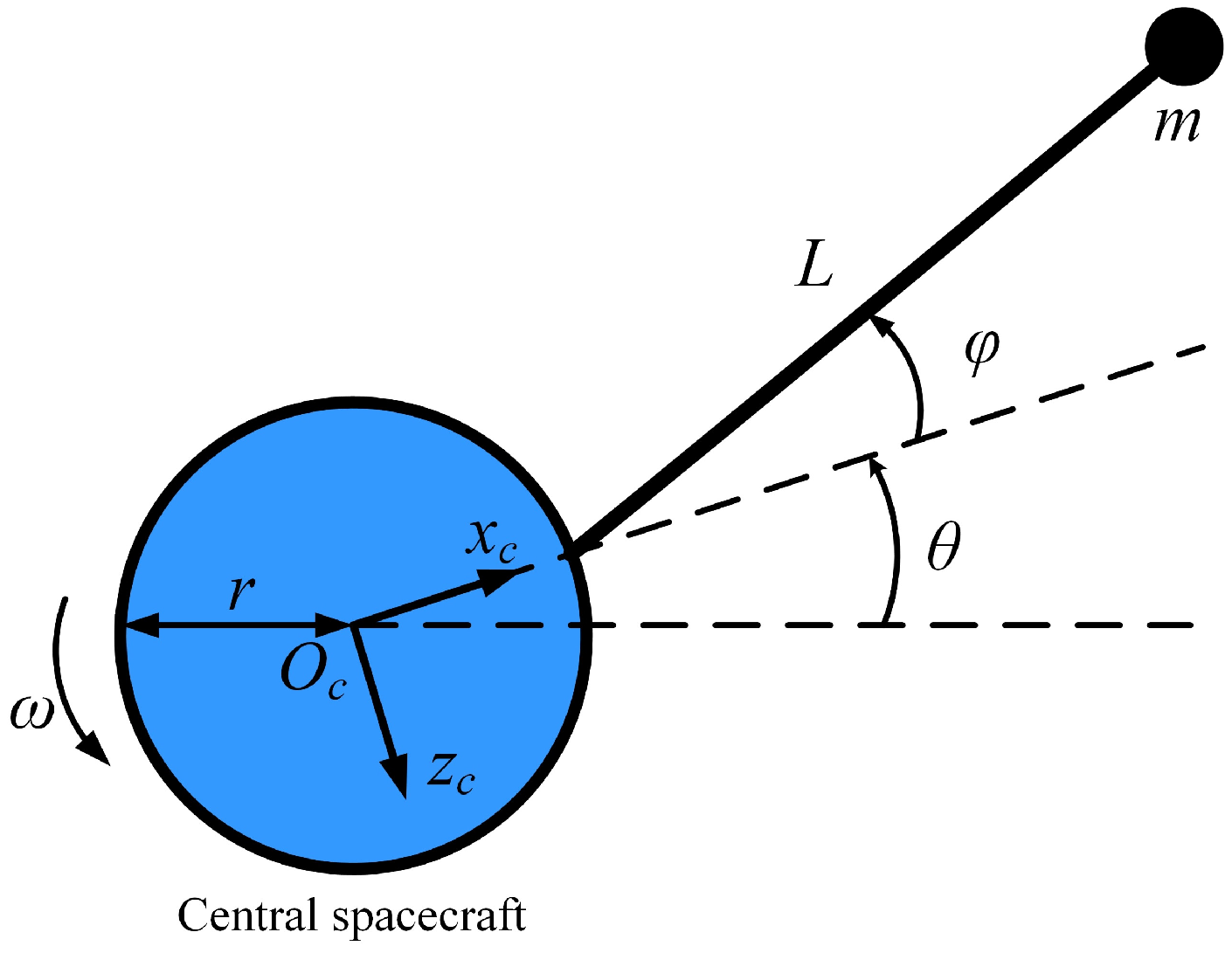
3.1. First Stage of Deployment

This subsection develops the deployment strategy based on a rigid dynamic model. The rationale is that, with appropriate deployment strategies, the spinning deployment of the STSS can maintain the tether in a tensioned state, thereby making its mechanical properties approach rigidity and significantly reducing the complexity of the deployment strategy design. However, if the tether becomes slack or undergoes large deformations, the deployment strategy designed based on the rigid model may become inapplicable. Therefore, the flexible dynamic model presented in Section 2 is employed to verify and analyze the deployment strategy, as described in Section 4.

For simplification, only one sub-satellite is considered and the system is modeled as a mass point, a rigid tether, and a rigid spacecraft. Figure 5 illustrates the parameters required for the radial deployment dynamics, where $\theta$ represents the rotational angle of the central spacecraft, $\omega$ represents the spinning angular velocity of the central spacecraft, $\phi$ represents the libration angle of the tether, namely the angle between the radial direction of the tether and the spacecraft, $m$ is the mass of the sub-satellite, $r$ is the radius of the spacecraft, and $L$ is the length of the tether.

According to the literature [24], the kinetic energy of the sub-satellite and the tether for this system is expressed using the following equation:

$$\begin{array}{l}K={\displaystyle \frac{1}{2}}(m+\rho L)r^2{\omega }^2+({\displaystyle \frac{m}{2}}+{\displaystyle \frac{\rho L}{8}}){v_1}^2+({\displaystyle \frac{m}{2}}+{\displaystyle \frac{\rho L}{6}})L^2{(\omega -\dot{\phi })}^2\\ +(m+{\displaystyle \frac{\rho L}{2}})rL\omega (\omega -\dot{\phi })\cos \phi -(m+{\displaystyle \frac{\rho L}{2}})r{v}_1\omega \sin \phi \end{array}$$

(40)

In a Lagrangian formulation without nonconservative forces, the governing equations arise from:

$${\displaystyle \frac{\mathrm{d}}{\mathrm{d}t}}\left({\displaystyle \frac{\partial K}{\partial \dot{\phi }}}\right)-{\displaystyle \frac{\partial K}{\partial \phi }}=0$$

(41)

Substituting Equation (40) into Equation (41), the governing equation can be expressed as

$$\begin{array}{l}\ddot{\phi }=\dot{\omega }+{\displaystyle \frac{1}{(m+\frac{\rho L}{3})L}}[(2m+\rho L)v_1(\omega -\dot{\phi })+(m+{\displaystyle \frac{\rho L}{2}})r\dot{\omega }\cos \phi \\ -(m+{\displaystyle \frac{\rho L}{2}})r{\omega }^2\sin \phi +{\displaystyle \frac{1}{2}}\rho r{v}_1\omega \cos \phi ]\end{array}$$

(42)

To achieve efficient deployment and decouple the equations of motion for deployment planning, the spacecraft is maintained at its initial high angular velocity. Concurrently, with the aim of preventing system instability caused by libration angle oscillations and ensuring the elimination of the initial libration angle during the deployment process, the libration angle is strategically planned. The initial libration angle is maintained during $t\in \left[0, t_t\right]$, after which it is linearly reduced to zero during $t\in \left[ t_t, t_d\right]$.

When $0\le t<t_t$, the libration angle is planned to be a constant value $\phi ={\phi }_0$. Substituting $\dot{\phi }=\ddot{\phi }=\dot{\omega }=0$ and $\phi ={\phi }_0$ into Equation (42), the following equation can be obtained:

$$0=(2m+\rho L)v_1\omega -(m+{\displaystyle \frac{\rho L}{2}})r{\omega }^2\sin {\phi }_0+{\displaystyle \frac{1}{2}}\rho r{v}_1\omega \cos {\phi }_0$$

(43)

According to Equation (43), the libration angle can be kept at the initial value by choosing the appropriate deployment velocity as

$$v_1=v_{1t}={\displaystyle \frac{(m+\frac{\rho L}{2})r\omega \sin {\phi }_0}{2m+\rho L+\frac{1}{2}\rho r\cos {\phi }_0}}$$

(44)

When $t_t\le t\le t_d$, a linear zeroing of the libration angle is implemented. Substituting $\dot{\phi }=\ddot{\phi }=\dot{\omega }=0$ and $\phi ={\phi }_0(1-{\displaystyle \frac{t-t_t}{t_d-t_t}})$ into Equation (42), then

$$0=(2m+\rho L)v_1\omega -(m+{\displaystyle \frac{\rho L}{2}})r{\omega }^2\sin \left[{\phi }_0(1-{\displaystyle \frac{t-t_t}{t_d-t_t}})\right]+{\displaystyle \frac{1}{2}}\rho r{v}_1\omega \cos \left[{\phi }_0(1-{\displaystyle \frac{t-t_t}{t_d-t_t}})\right]$$

(45)

According to Equation (45), the libration angle can be linearly brought to zero by choosing the deployment velocity as

$$v_1=v_{1d}={\displaystyle \frac{(m+\frac{\rho L}{2})r\omega \sin \left[{\phi }_0(1-\frac{t-t_t}{t_d-t_t})\right]}{2m+\rho L+\frac{1}{2}\rho r\cos \left[{\phi }_0(1-\frac{t-t_t}{t_d-t_t})\right]}}$$

(46)

The linear elimination process of the libration angle begins when the length of the tether is at a certain ratio of the final length during the first deployment stage, namely $L_t=\beta L_d$, where $\beta$ is the deceleration factor. To maintain a constant spinning rate throughout this stage, a proportional-derivative (PD) control torque is applied to the central spacecraft. The control law adjusts the spacecraft’s angular velocity based on the error between the desired and actual states, ensuring stable deployment dynamics.

3.2. Second Stage of Deployment

A strategy for the second stage of deployment is presented in this section to address the safety challenges associated with the rapid increase in tether tension during the first stage of deployment, caused by the constant high angular velocity and the extension of the tether. If there is no driving torque applied to the central spacecraft, the angular velocity of the STSS will gradually decrease with tether extension due to system angular momentum conservation. This implies that the tension of the tether will also reduce over time, ensuring that the tension remains within a safe range as the tether continues to extend. However, if the rotation of the central spacecraft is completely uncontrolled, the libration angle will continuously increase and cannot be stabilized within a small range. Therefore, by applying an active driving torque to the central spacecraft to align its spinning angular velocity with the rotational speed of the sub-satellite relative to the central spacecraft, a good synchronization between the rotation of the central spacecraft and the sub-satellite can be maintained to eliminate the libration angle. This strategy ensures the libration angle within a narrow range and guarantees the secure deployment of the tether system to its final length.

The safe deployment length of the tether is calculated below to facilitate the division of the deployment stages. The tensile strength of material is characterized by

$$\sigma =F_b/A$$

(47)

where $\sigma$ represents the tensile strength and $F_b$ is the maximum tension endured by the tether until it breaks.

To ensure a sufficient safety margin, especially considering the complex spatial environment that may introduce additional stresses, a safety factor $S$ is commonly implemented. $F_p$ represents the allowable stress and is given by

$$F_p=F_b/S$$

(48)

Considering the mass of the tether and treating the tether as a rigid rod, the maximum tension of the tether, occurring at the connection point with the central spacecraft, can then be calculated as

$$F_t=r\cos \phi {\omega }^2(m+\rho L)+L{(\dot{\phi }+\omega )}^2(m+{\displaystyle \frac{\rho L}{2}})$$

(49)

During the first stage of deployment, the tension in the tether system increases with the extension of the tether because of the constant spinning angular velocity of the central spacecraft. Therefore, at the end of the first stage, the tension in the tether system is at a maximum value and the tether length is $L=L_d$ at this time. According to Equations (48) and (49) and the conditions $\phi =\dot{\phi }=0$, we obtain

$${\displaystyle \frac{1}{2}}\rho {\omega }^2{L_d}^2+\left(m+\rho r\right){\omega }^2{L}_d+mr{\omega }^2-F_p=0$$

(50)

Equation (50) can be used to determine tether length $L_d$ at the beginning of the second stage of deployment, during which the tether deployment velocity remains constant. The rotational motion of the central spacecraft is continuously adjusted to match the sub-satellite’s relative position and velocity, ensuring the stability of libration angle throughout the remaining deployment. The control torque acting on the central spacecraft during this stage is denoted as

$$T=K_p(\theta -{\theta }_s)+K_d(\omega -{\omega }_s)$$

(51)

where ${\theta }_s$ and ${\omega }_s$ represent the rotational angle and rotational speed of the sub-satellite relative to the central spacecraft, respectively.

4. Simulation and Analysis

This section is divided into four subsections to analyze the deployment process of the STSS based on the dynamic model in Section 2 and the staged deployment strategy in Section 3. Section 4.1 verifies the accuracy of the dynamic model through a fundamental case. To validate the deployment strategy deduced by the single-satellite model, Section 4.2 presents a numerical simulation of the dynamics and control of the STSS deployment process using a single sub-satellite configuration with the spin axis of the central spacecraft constrained and space environmental forces neglected. Section 4.3 refines the deployment strategy to address the issues identified in the first subsection. Furthermore, to evaluate the feasibility of applying this strategy to a multi-satellite tethered system, Section 4.4 investigates the effects of the deployment strategy within the space environment using a twin sub-satellite configuration. This analysis examines how different orientations of the STSS influence the deployment process and compensates for space environmental forces to achieve improved deployment outcomes. The simulation parameters of the STSS used throughout these subsections are listed in

Table 1. Parameters of the STSS.

Parameters	Value	Units
Principal inertia of central spacecraft	(200, 200, 200)	kg·m2
Principal inertia of sub-satellite	(0.02, 0.02, 0.02)	kg·m2
Mass of central spacecraft	1500	kg
Mass of sub-satellite	5	kg
Radius of central spacecraft	0.5	m
Linear density of tether	0.02607	kg/m
Diameter of tether	2	mm
Elastic modulus of tether	128	GPa
Tensile strength of tether	827	MPa
Total tether length	800	m
Threshold length of tether element	50	m
Initial spinning angular velocity	1	rad/s
Initial libration angle	π/6	rad

.

4.1. Dynamic Model Validation

To validate the flexible model accuracy in Section 2, a fundamental STSS operational scenario is selected for investigation and rigorously verified through simulation analysis. This analysis employs a single sub-satellite configuration and neglects space environmental forces.

The case unfolds in three stages: (1) a 100-s steady-state spin, (2) a spin-up maneuver via a 2 Nm thruster torque applied over 100 s, and (3) a 300-s stabilization period. The tether length is set as 20 m. As shown in Figure 6a, the system maintains dynamic equilibrium during the steady-state spin, characterized by constant angular momentum (2376 kg·m²/s). When the 2 Nm torque is applied, angular momentum increases to 2576 kg·m²/s over 100 s. The angular momentum increment of 200 kg·m²/s exactly equals the angular impulse over this period. Notably, the flexible tether and sub-satellite exhibit phase lag relative to the central spacecraft during torque application, generating a libration angle that induces periodic fluctuations post-maneuver, as documented in Figure 6b.

Figure 6c shows that the libration angle introduces periodic angular velocity oscillations for the central spacecraft, as evident in the waveform. The average angular velocity increases by 0.084 rad/s, which is equivalent to the angular momentum increment divided by the system moment of inertia. Figure 6d demonstrates that tether tension increases with angular velocity, while the libration angle causes superimposed periodic tension variations, reflecting the coupled dynamics of rotational acceleration and tether flexibility.

The simulations validate the model’s accuracy in predicting angular momentum conservation or variation, as well as dynamic behaviors, including libration, angular velocity, and tension fluctuations, confirming close alignment with theoretical predictions.

4.2. Single Sub-Satellite Configuration Without Space Environmental Forces

In the first stage of deployment, a high spinning angular velocity of the central spacecraft is employed to ensure efficient deployment; the tether deployment velocity is planned based on Equations (44) and (46), where the deceleration factor is $\beta =0.8$. Once the tether reaches the maximum safe length $L_d$ under tension constraints, the system transitions from the first to the second stage of deployment, where the safety factor is set as $S=1.5$. In the second stage of deployment, the tether deployment velocity is planned to be a constant value; the angular velocity of the central spacecraft synchronizes with the sub-satellite. A numerical simulation is conducted using the model in Section 2 that considers the flexibility of the tether, and this model is compared with the traditional rigid model [26].

Figure 7 illustrates the variation curve of the tether deployment velocity in different stages. During the first stage of deployment, the tether deployment initially approaches a constant velocity for a period of time before linearly decelerating to zero. During the second stage of deployment, the tether deployment velocity remains 0.3 m/s. When the maximum length of the tether is reached, the deployment velocity is reduced to zero and the STSS enters a stable stage.

Figure 8 presents the spinning angular velocity of the central spacecraft when the staged deployment strategy is applied to both the rigid and flexible models. During the first stage of deployment, the angular velocity is controlled near 1 rad/s. However, compared with the rigid model, the angular velocity curve in the flexible model has obvious oscillation, which is due to the fact that the flexible deformation of the tether causes the oscillating tension to react on the central spacecraft. Therefore, the flexible model can more accurately reflect the vibration characteristics of the STSS. In the second stage of deployment, the angular velocity of the central spacecraft is no longer controlled to a constant value, but it is controlled to synchronize with the rotational speed of the sub-satellite relative to the central spacecraft. The angular velocities of both the rigid and flexible models are gradually reduced because of the increasing moment of inertia with the deployment of the tether, and the angular velocity during the second stage of deployment is lower in the flexible model than in the rigid model due to the consideration of the tether mass. In the stable stage, the angular velocity of the central spacecraft remains almost constant.

Figure 9 illustrates the variation in tether length. After the staged deployment with the deployment velocity in Figure 7, the tether finally expanded to the maximum length of 800 m. Although the rigid and flexible models have the same tether deployment velocity, it is clear that the tether length of the flexible model is slightly larger than that of the rigid model, which is particularly obvious in the first stage of deployment. This is due to the higher spinning angular velocity of the system relative to other stages, which leads to the larger tension and tensile deformation in the tether. In the stable stage, the tether length of the flexible model is close to that of the rigid model because of the low spinning angular velocity of the system, but there are obvious oscillations. This is due to the swing of the tether after entering the stable stage, which can be seen from the curve of the libration angle in Figure 12.

Figure 10 depicts the control torque applied to the central spacecraft throughout the deployment process. During the first stage of deployment, the control torque is used to maintain a consistent spinning angular velocity of the central spacecraft. As the tether extends at a nearly constant velocity, the control torque gradually increases with the increasing of the moment of inertia of the STSS. Beyond $t=1977 \mathrm{s}$, the control torque gradually decreases as the tether deployment velocity decreases. Compared with the rigid model, the control torque of the flexible model is greater due to the consideration of tether mass. In the second stage of deployment, the rotation of the central spacecraft and the sub-satellite can be synchronized with small control torques. However, compared with the rigid model, the control torque of the flexible model is larger and there exists complex oscillations.

Figure 11 shows the tension variation curves of the tether at the connection between the tether and the central spacecraft. The single-stage deployment results in tether tension exceeding the allowable stress (Figure 11a), while the staged deployment shows controlled tension variation (Figure 11b). In the first stage of deployment, the tether tension gradually increases owing to the increased length of the tether under a constant spinning angular velocity. In the second stage of deployment, the tether tension gradually decreases with the decrease in system spinning angular velocity, which avoids the possible tether fracture caused by the continuous increase of tether tension. Furthermore, there exists oscillations in the tether tension of the flexible model. In the stable stage, the tether tension remains almost unchanged, where the flexible model continues to exhibit slight oscillations in the tether tension.

Figure 12 presents a comparison of the libration angle between the rigid model and the flexible model. The rigid model maintains the initial libration angle in the first part of the deployment stage and achieves a libration angle of zero in the latter part of this stage. The simulated libration angle is in agreement with the theoretical result obtained from the proposed strategy, which indicates the ability of the control strategy to achieve good rotational synchronization between the central spacecraft and the sub-satellite, ensuring the stability of the STSS. However, the variation of the libration angle of the flexible model is more complicated compared with that of the rigid model. The flexible model exhibits larger amplitude and requires longer time for the angles to converge. Even in the stable stage after deployment, the libration angle of the tether still fluctuates persistently.

Figure 13 illustrates the motion trajectory of the sub-satellite relative to the central spacecraft. Since the trajectories of the rigid and flexible models are similar, only the result of the flexible model is presented here. The trajectory is a gradually increasing curvature arc, and the density of the trajectory can reflect the ratio of the tether deployment velocity to the system spinning angular velocity. The high spinning angular velocity of the system in the first stage leads to a dense trajectory. After entering the second stage, the trajectory gradually becomes sparse due to the decrease of the spinning angular velocity.

The above simulation results demonstrate the effectiveness of the proposed staged deployment strategy and the importance of using the flexible model to analyze the dynamic behavior of the STSS. When utilizing the flexible model, obvious libration angle fluctuations occur during the onset of the first stage, followed by persistent oscillations in libration angle during the stable stage after completing the deployment process. These dynamic behaviors compromise the stability of the STSS. Therefore, the deployment strategy needs to be further optimized.

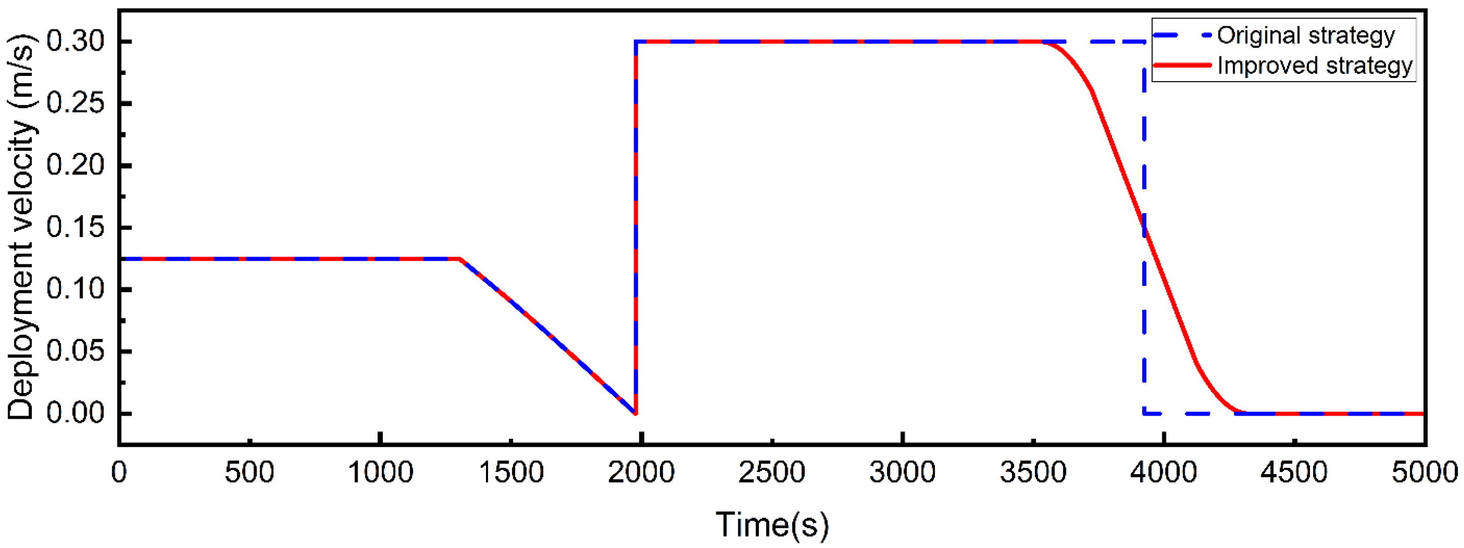
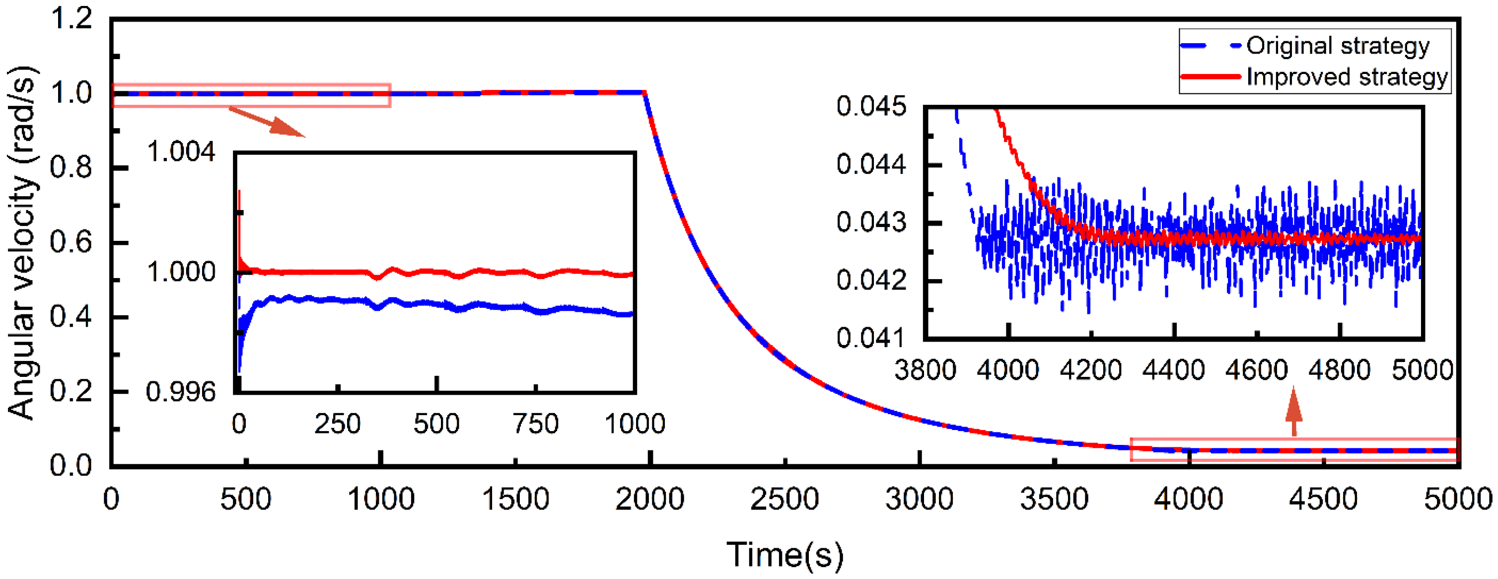
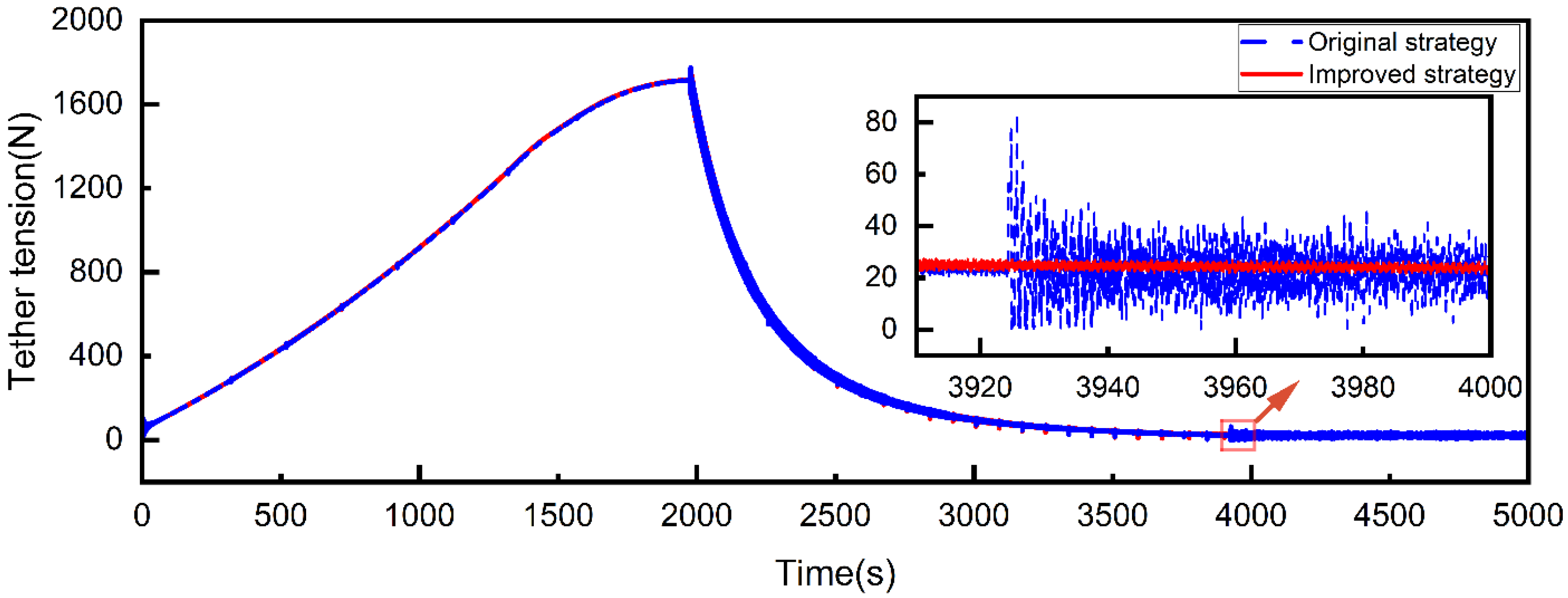
4.3. Single Sub-Satellite Configuration with an Improved Staged Deployment Strategy

Although PD control demonstrates commendable performance in many applications, PD controllers rely on fixed parameters and are unable to adaptively adjust to dynamic changes in the system, which can degrade control performances, especially in systems with time-varying or uncertain dynamics. To address the limitations of PD control, compensation of the torque acting on the central spacecraft by the tether can be introduced during the first deployment stage for libration angle maintenance. The expression for the driving torque is

$$T=K_p(\theta -{\theta }_d)+K_d(\omega -{\omega }_d)+F_{con}r\sin \phi$$

(52)

where $F_{con}$ represents the tension of the tether acting on the spacecraft at the connection point, expressed as $F_{con}=EA({\epsilon }_c+c{\dot{\epsilon }}_c)$. Here, ${\epsilon }_c$ denotes the tensile strain at the connection point.

Additionally, a smooth transition in the deployment velocity is implemented before the stable stage instead of a step change. This is achieved through the utilization of a staged transition function as follows:

$$v_k=\left\{\begin{array}{c}{v}_f\cos ({\displaystyle \frac{2\pi (t-t_a)}{3t_k}}) (t_a\le t<t_b)\\ {\displaystyle \frac{2(1-\sqrt{3})v_f}{t_k}}(t-t_b)+{\displaystyle \frac{\sqrt{3}{v}_f}{2}} (t_b\le t<t_c)\\ v_f\cos ({\displaystyle \frac{2\pi (t-t_c)}{3t_k}}+{\displaystyle \frac{5\pi }{6}})+v_f (t_c\le t<t_f)\end{array}\right.$$

(53)

where $t_a=t_f-t_k$, $t_b=t_f-{\displaystyle \frac{3}{4}}{t}_k$, $t_c=t_f-{\displaystyle \frac{1}{4}}{t}_k$, $v_k$ represents the smooth transition deployment velocity of the tether, and $t_k$ is the time duration for the smooth transition.

The improved staged deployment strategy is employed for simulation and analysis of the flexible model, where $t_k=800 \mathrm{s}$, $v_f=0.3 \mathrm{m}/\mathrm{s}$, and the other parameters are the same as in the previous subsection. The deployment velocity of the tether during the staged deployment process, as depicted in Figure 14, exhibits a smooth transition before completing tether deployment.

In Figure 15, the libration angle of the flexible model under the improved and original staged deployment strategies is depicted. The result illustrates that the inclusion of the compensatory moment in the PD control substantially reduces the initial fluctuations in the libration angle. Furthermore, the implementation of the transition in tether deployment velocity corrects the deflection of libration angle during the stable stage, and there is no longer obvious fluctuation in the libration angle compared with the result of the original strategy.

The improvement of SSTS deployment stability using the improved strategy can also be seen from the curves of the spinning angular velocity of the central spacecraft and the tether tension, as shown in Figure 16 and Figure 17. In the first stage, the angular velocity of the central spacecraft under the improved strategy is closer to the expected 1 rad/s than that of the original strategy. This is because the tether tension compensation is introduced into the control torque, which reduces the steady-state error of the angular velocity. Due to the introduction of the smooth transition in the deployment velocity before the end of deployment, there are no longer significant fluctuations in the angular velocity of the central spacecraft and tether tension during the stable stage.

By optimizing torque control and deployment velocity, this section effectively eliminates libration angle oscillations and consequent tension and angular velocity fluctuations, which improves the overall stability of the system during the deployment and stable stages. Therefore, the improved staged deployment strategy is more reliable than its original counterpart in achieving the desired stable state of the STSS.

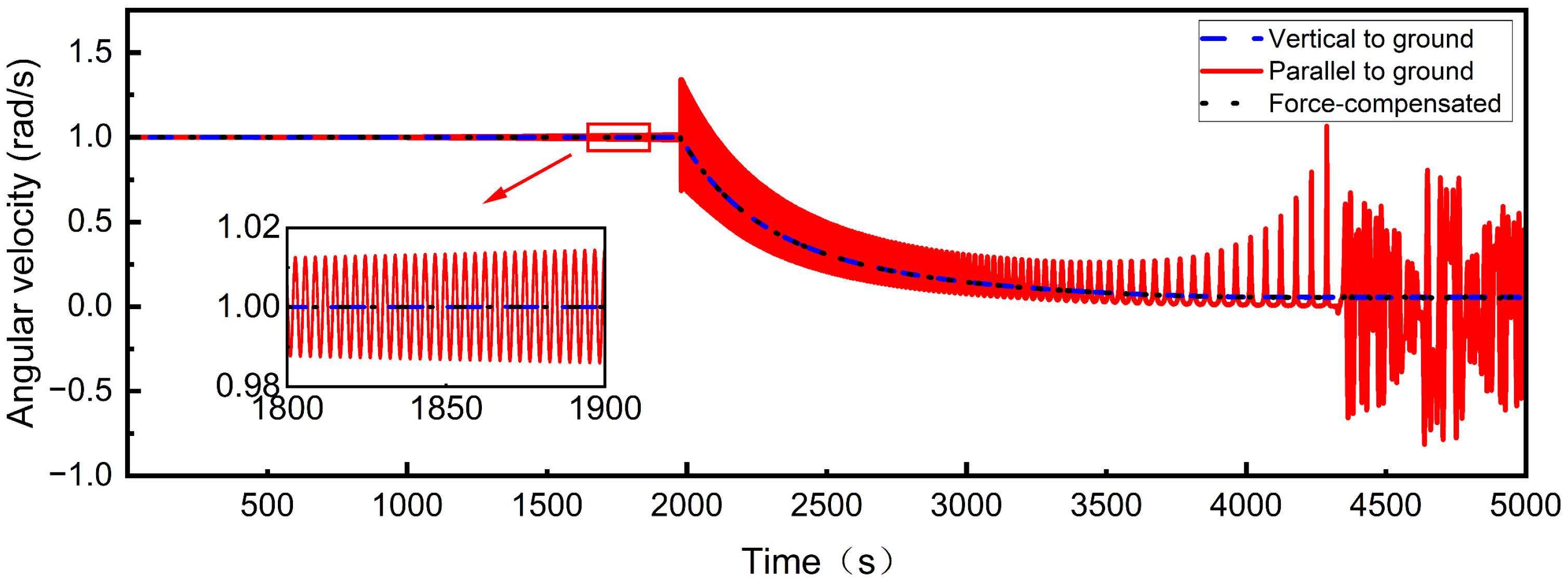
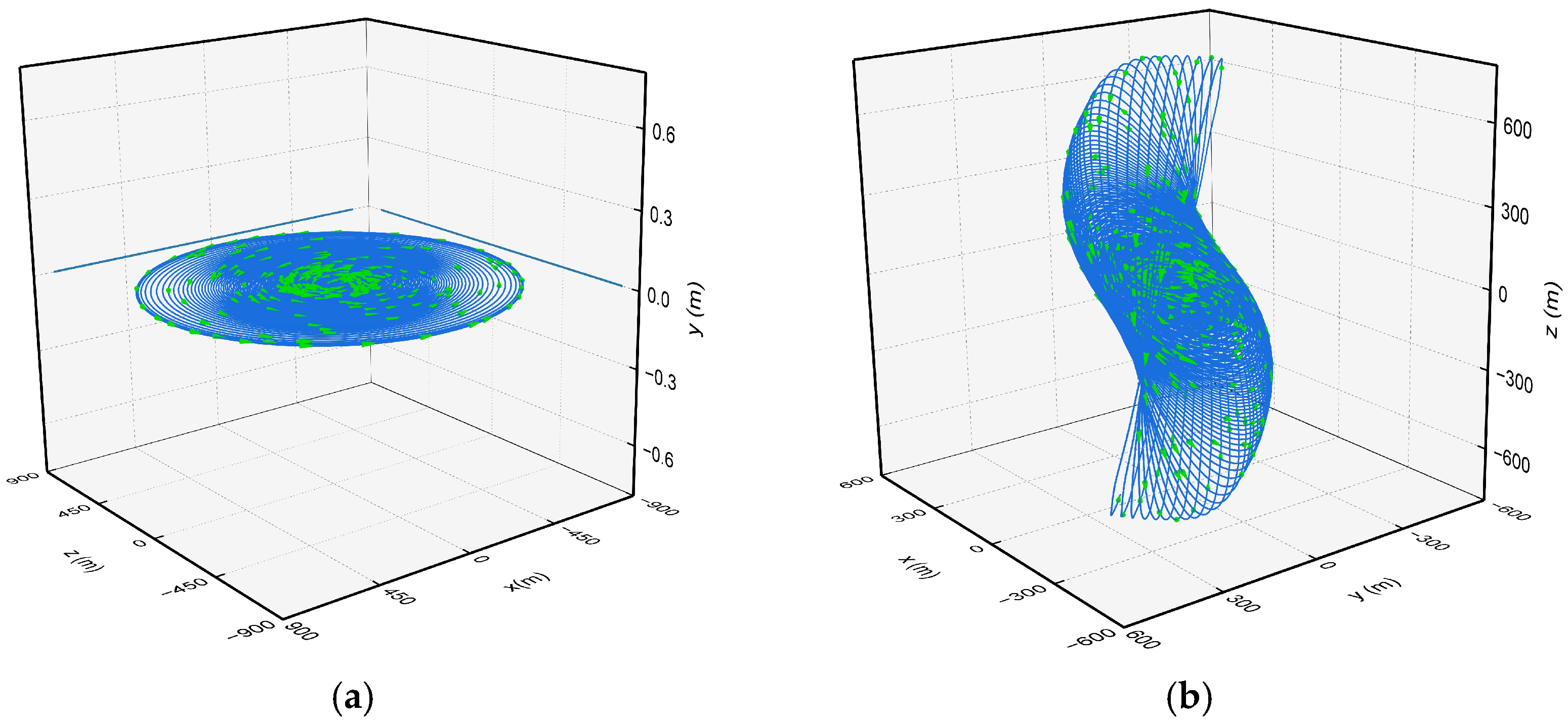
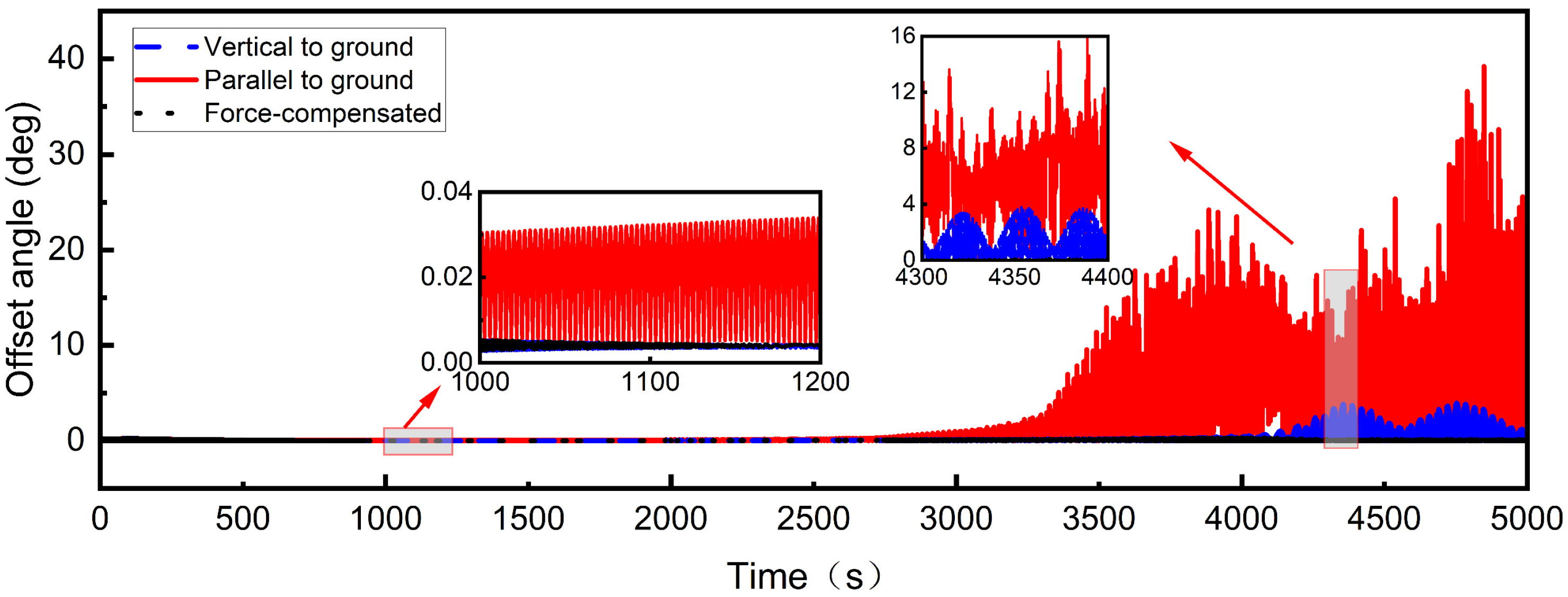
4.4. Twin Sub-Satellite Configuration Considering Space Environmental Forces

In this subsection, the staged deployment process of the twin sub-satellite configuration is further analyzed, taking into account the effects of space environmental forces in geostationary orbit. Three deployment cases are considered. In the vertical-to-ground case, the spin plane is initially vertical to the Earth’s surface. In the parallel-to-ground case, the spin plane is initially parallel to the Earth’s surface, and the spin axis of the central spacecraft is constrained to avoid attitude disturbances caused by the Dzhanibekov effect, which would otherwise cause drastic attitude changes [21]. In the force-compensated case, space environment forces are compensated throughout the deployment process. This involves applying forces to the satellites that are opposite to space environmental forces, effectively offsetting these disturbances. In these cases, the tethers are attached 0.1 m from the centroids to the edges of the sub-satellites, rather than at their centroids. For the subsequent analysis, one sub-satellite will be selected for detailed investigation.

The rationale for considering these specific cases (vertical-to-ground and parallel-to-ground) is to demonstrate the influence of two primary space environmental disturbance forces: the gravity gradient force and the Coriolis force. Furthermore, these cases correspond to common scenarios in space missions, such as Earth observation and orbital deployment, with other orientations generally falling between these two extremes. This approach ensures a systematic analysis of environmental factors’ impact on deployment dynamics while covering representative mission configurations, thereby enhancing the strategy’s applicability.

Figure 18 depicts the variation in the spinning angular velocity of the central spacecraft. In the vertical-to-ground case, the angular velocity consistently approaches the ideal state throughout the deployment process. In the parallel-to-ground case, the angular velocity oscillates around 1 rad/s during the first stage of deployment, with the amplitude gradually increasing. In the second stage, the angular velocity undergoes significant oscillation. Post-deployment, the oscillations intensify, with alternating forward and reverse rotations, indicating that the angular velocity control is challenging in this case. In the force-compensated case, severe oscillations in angular velocity are effectively prevented.

Figure 19, Figure 20 and Figure 21 illustrate the motion of the sub-satellite relative to the central spacecraft under different deployment cases. In the vertical-to-ground case, Figure 19a shows that the trajectory of the sub-satellite remains within the initial spin plane, indicating the absence of out-of-plane space environmental forces and hence no out-of-plane motion. Consequently, Figure 20 shows that the out-of-plane angle $\gamma$ remains at zero. Additionally, due to effective control of the angular velocity of the central spacecraft, the libration angle in Figure 21 is well maintained along the desired trajectory, despite minor fluctuations induced by Coriolis and gravitational gradient forces.

In the parallel-to-ground case, as shown in Figure 19b, the Coriolis and gravitational gradient forces cause the sub-satellites to deviate from the initial spin plane, resulting in a complex three-dimensional helical trajectory. This deviation is further evidenced in Figure 20, where the out-of-plane angle gradually increases during the first deployment stage. In the second stage, the oscillation frequency of the angle decreases due to the increased tether deployment velocity and decreased angular velocity. Additionally, as depicted in Figure 21, while the libration angle initially follows the desired control trajectory, its oscillation amplitude gradually increases. In the second stage, the libration angle fails to converge to zero, and during the stable stage significant out-of-plane motion couples with in-plane motion, causing large fluctuations in the libration angle and ultimately compromising the stability of the STSS.

In the force-compensated case, compensating for space environmental forces effectively suppresses the oscillations in both the libration angle and the out-of-plane angle. As depicted in Figure 19 and Figure 20, the out-of-plane angle approaches zero and the libration angle remains stable, resulting in an optimal deployment process.

To describe the stability of the attitude of sub-satellites during deployment, the offset angle ${\theta }_{\mathrm{o}}$ is introduced. The offset angle is defined as the angle between the tether and the vector from the centroid of the sub-satellite to the attachment point, as illustrated in Figure 1. Figure 22 demonstrates the variation of the offset angle under three different cases. In the vertical-to-ground case, the amplitude of the offset angle remains small throughout the deployment process but exhibits periodic fluctuations of approximately 4° during the stable stage. In the parallel-to-ground case, the amplitude of the offset angle gradually increases during deployment, reaching nearly 40° with aperiodic fluctuations during the stable stage. With the implementation of the environmental force compensation strategy, the offset angle of the sub-satellite is effectively suppressed.

Treating the STSS composed of the central spacecraft, sub-satellites, and tether as an integrated system, its stability can be analyzed via the spin-stabilization and gravity-gradient stabilization conditions of the spacecraft. Since the system’s spin axis aligns with the maximum principal inertia axis, it satisfies the spin-stabilization prerequisites in the inertial space. However, in the orbital frame, the Coriolis force induces out-of-plane motion when a misalignment exists between the spin plane and orbital plane—for example, in the parallel-to-ground scenario. The impacts of gravity gradient on the system stability in the two scenarios are different. The spacecraft achieves stability when its long axis (minimum principal inertia axis) points toward the Earth’s center. In the parallel-to-ground case, however, the maximum principal inertia axis is oriented toward the Earth, rendering the system unstable. This instability induces out-of-plane motion and subsequent system attitude deflection, as illustrated in Figure 19. In the vertical-to-ground case, when the tether initially points toward the Earth’s center, the system resides in a gravity-gradient stable state. During spinning, the gravity-gradient force and Coriolis force remain within the spin plane, ensuring sustained system stability.

In summary, for the vertical-to-ground case, the staged deployment strategy demonstrates stable performance. However, in the parallel-to-ground case, the STSS exhibits significant instabilities in the in-plane libration angle, out-of-plane angle, and satellites attitude due to the complex influence of the gravitational gradient force and the Coriolis force. Therefore, compensating for space environmental forces in this case can effectively mitigate these issues, ensuring stable deployment.

5. Conclusions

The dynamic modeling and deployment strategy of STSSs are studied in this paper, and the conclusions are summarized as follows:

(1)

A multibody dynamic model is developed to analyze the nonlinear characteristics of the STSS deployment process, employing the ANCF within an ALE framework in conjunction with Lagrange multipliers. This model effectively captures the flexibility and length variation of the tether, as well as the attitude of the satellites. Both the gravitational gradient force and the Coriolis force are taken into account. Unlike the traditional massless/rigid rod model, the tether in this model is discretized into multiple flexible elements, accounting for both axial and bending deformations, thereby significantly enhancing the accuracy in characterizing the tether’s behavior.

(2)

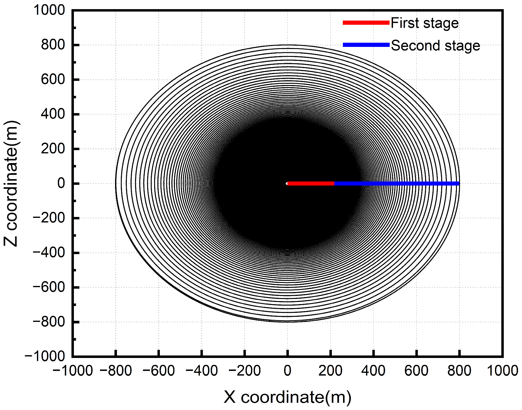
A staged deployment control strategy based on safety tension division is proposed to address the problem of mutual restriction between high-speed spin and tether tension in the STSS. In the first stage, a high spinning angular velocity of the central spacecraft and the deployment velocity of the tether are planned to ensure deployment efficiency, and meanwhile eliminating the libration angle and oscillations in the STSS. Moreover, a method for calculating maximum tether tension is proposed to divide the deployment stage. When the tether tension exceeds the maximum critical value, the deployment enters the second stage. In this stage, the tether tension can be gradually reduced with the decrease of the spinning angular velocity of the STSS, which ensures the safety of the deployment process.

(3)

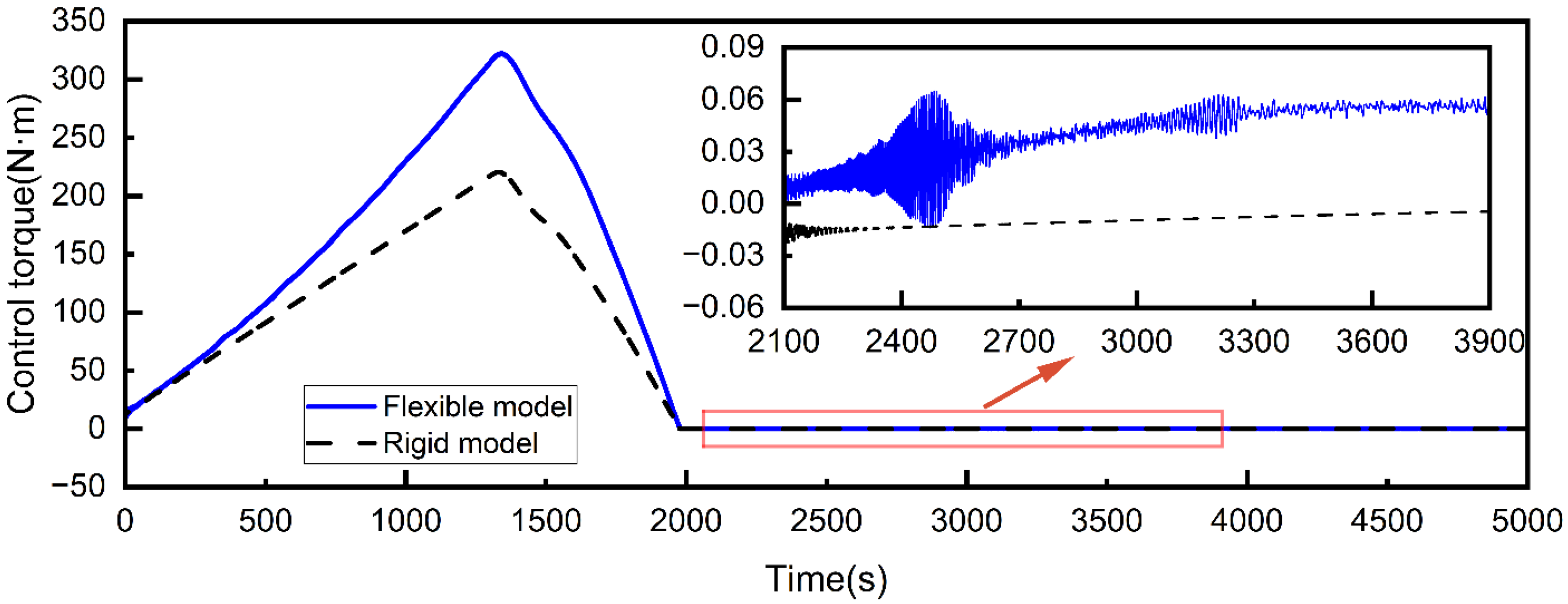
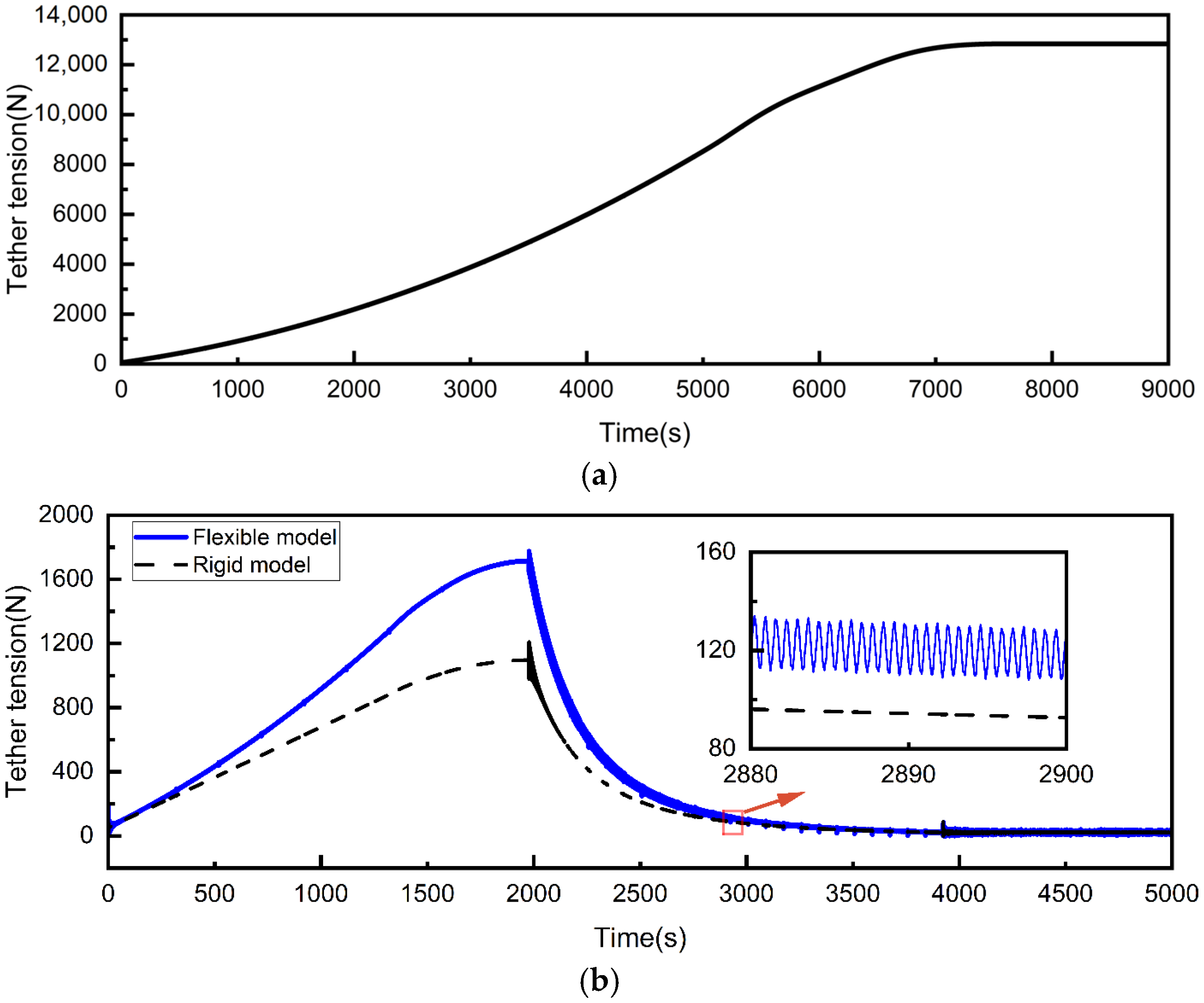
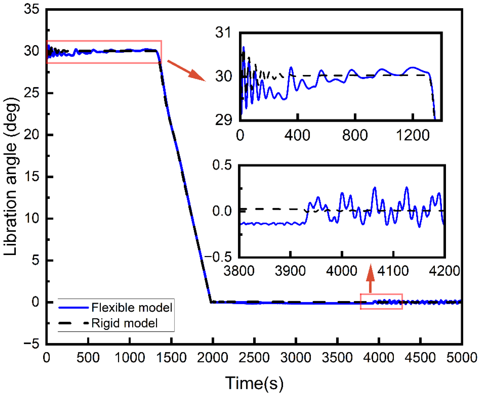
Simulation results indicate that, when considering flexibility, the STSS exhibits greater oscillations in dynamic responses, such as libration angle and tether tension. Therefore, the application of the flexible model is essential to accurately reflect the vibration characteristics and dynamic behavior of the STSS. The accuracy of the dynamic model and the effectiveness of the proposed staged deployment strategy are demonstrated by numerical simulations, and torque compensation and deployment velocity transitions are introduced to mitigate libration angle fluctuations, thereby optimizing the dynamic performance of the STSS during deployment. Furthermore, the analysis of deployment dynamics under space environmental forces reveals that, while the STSS in vertical-to-ground orientation remains stable, the STSS in parallel-to-ground orientation experiences significant instabilities, reflected in fluctuations of the libration angle, out-of-plane angle, and attitude of the satellites. These instabilities can be effectively mitigated through space force compensation.

References

1. Huang, P.; Zhang, F.; Chen, L.; Meng, Z.; Zhang, Y.; Liu, Z.; Hu, Y. A review of space tether in new applications. Nonlinear Dyn. 2018, 94, 1–19. [Google Scholar] [CrossRef]
2. Ma, Y.; Ge, R.; Xu, M. Design concept of a tethered satellite cluster system. Aerosp. Sci. Technol. 2020, 106, 106159. [Google Scholar] [CrossRef]
3. Selva, D.; Golkar, A.; Korobova, O.; i Cruz, I.L.; Collopy, P.; de Weck, O.L. Distributed Earth Satellite Systems: What Is Needed to Move Forward? J. Aerosp. Inf. Syst. 2017, 14, 412–438. [Google Scholar] [CrossRef]
4. Lu, H.; Li, A.; Wang, C.; Zabolotnov, Y.M. Tether Deformation of Spinning Electrodynamic Tether System and Its Suppression with Optimal Controller. J. Aerosp. Eng. 2021, 34, 04021003. [Google Scholar] [CrossRef]
5. Shan, M.; Shi, L. Comparison of Tethered Post-Capture System Models for Space Debris Removal. Aerospace 2022, 9, 33. [Google Scholar] [CrossRef]
6. Jiang, X.; Bai, Z. Dynamic analysis of the tethered satellite system considering uncertain but bounded parameters. Def. Technol. 2024, 42, 116–124. [Google Scholar] [CrossRef]
7. Misra, A.K.; Nixon, M.S.; Modi, V.J. Nonlinear Dynamics of Two-Body Tethered Satellite Systems: Constant Length Case. J. Astronaut. Sci. 2001, 49, 219–236. [Google Scholar] [CrossRef]
8. Luo, C.; Wen, H.; Jin, D.; Xu, S. Long-term deorbiting control for an electrodynamic tether system exploiting periodic solutions. Acta Astronaut. 2023, 202, 174–185. [Google Scholar] [CrossRef]
9. Beletsky, V.; Kasatkin, G.; Starostin, E. The pendulum as a dynamical billiard. Chaos Solitons Fractals 1996, 7, 1145–1178. [Google Scholar] [CrossRef]
10. Hongshi, L.; Hang, Y.; Changqing, W.; Aijun, L. Nonlinear deformation and attitude control for spinning electrodynamic tether systems during spin-up stage. Nonlinear Dyn. 2024, 112, 7011–7027. [Google Scholar] [CrossRef]
11. No, T.S.; Cochran, J.E. Dynamics and Control of a Tethered Flight Vehicle. J. Guid. Control. Dyn. 1995, 18, 66–72. [Google Scholar] [CrossRef]
12. Fotland, G.; Haugen, B. Numerical integration algorithms and constraint formulations for an ALE-ANCF cable element. Mech. Mach. Theory 2022, 170, 104659. [Google Scholar] [CrossRef]
13. Escalona, J.L. An arbitrary lagrangian–eulerian discretization method for modeling and simulation of reeving systems in multibody dynamics. Mech. Mach. Theory 2017, 112, 1–21. [Google Scholar] [CrossRef]
14. Sun, J.; Tian, Q.; Hu, H.; Pedersen, N.L. Simultaneous topology and size optimization of a 3D variable-length structure described by the ALE–ANCF. Mech. Mach. Theory 2018, 129, 80–105. [Google Scholar] [CrossRef]
15. Shabana, A.A. Flexible multibody dynamics: Review of past and recent developments. Multibody Syst. Dyn. 1997, 1, 189–222. [Google Scholar] [CrossRef]
16. Shan, M.; Guo, J.; Gill, E. Deployment dynamics of tethered-net for space debris removal. Acta Astronaut. 2017, 132, 293–302. [Google Scholar] [CrossRef]
17. Tang, J.; Ren, G.; Zhu, W.; Ren, H. Dynamics of variable-length tethers with application to tethered satellite deployment. Commun. Nonlinear Sci. Numer. Simul. 2011, 16, 3411–3424. [Google Scholar] [CrossRef]
18. Zhang, Y.; Jiang, X.; Bai, Z.-F.; Guo, J.-W.; Wei, C. Dynamics and rebound behavior analysis of flexible tethered satellite system in deployment and station-keeping phases. Def. Technol. 2022, 18, 509–523. [Google Scholar] [CrossRef]
19. Wang, R.; Wei, C.; Wu, Y.; Zhao, Y. The Study of Spin Control of Flexible Electric Sail Using the Absolute Nodal Coordinate Formulation. In Proceedings of the 2017 IEEE International Conference on Cybernetics and Intelligent Systems (CIS) and IEEE Conference on Robotics, Automation and Mechatronics (RAM), Ningbo, China, 19–21 November 2017; IEEE: New York, NY, USA, 2017; pp. 785–790. [Google Scholar]
20. Luo, C.; Sun, J.; Wen, H.; Jin, D. Dynamics of a tethered satellite formation for space exploration modeled via ANCF. Acta Astronaut. 2020, 177, 882–890. [Google Scholar] [CrossRef]
21. Sun, J.; Chen, E.; Chen, T.; Jin, D. Spin dynamics of a long tethered sub-satellite system in geostationary orbit. Acta Astronaut. 2022, 195, 12–26. [Google Scholar] [CrossRef]
22. Du, C.; Zhu, Z.H. Dynamic characterization and sail angle control of electric solar wind sail by high-fidelity tether dynamics. Acta Astronaut. 2021, 189, 504–513. [Google Scholar] [CrossRef]
23. Trushlyakov, V.I.; Yudintsev, V.V. Rotary space tether system for active debris removal. J. Guid. Control Dyn. 2020, 43, 354–364. [Google Scholar] [CrossRef]
24. Tragesser, S.G.; Gorjidooz, B. Open-loop spinup and deployment control of a tether sling. J. Spacecr. Rocket. 2010, 47, 345–352. [Google Scholar] [CrossRef]
25. Huang, P.; Zhao, Y.; Zhang, F.; Ma, J.; Meng, Z.; Liu, Z.; Zhang, Y. Deployment/retraction of the rotating Hub-Spoke Tethered Formation System. Aerosp. Sci. Technol. 2017, 69, 495–503. [Google Scholar] [CrossRef]
26. Zhai, G.; Su, F.; Zhang, J.; Liang, B. Deployment strategies for planar multi-tethered satellite formation. Aerosp. Sci. Technol. 2017, 71, 475–484. [Google Scholar] [CrossRef]
27. Fulton, J.; Schaub, H. Fixed-axis electric sail deployment dynamics analysis using hub-mounted momentum control. Acta Astronaut. 2018, 144, 160–170. [Google Scholar] [CrossRef]
28. Liu, C.; Wang, W.; Kang, J.; Zhu, Z.H. Spin deployment of Hub-Spoke tethered satellite formation with sliding mode tether tension control. Adv. Space Res. 2023, 71, 2509–2520. [Google Scholar] [CrossRef]
29. Su, F.; Zhai, G.; Zhang, J.; Zhang, Y. Dynamics and control during spinning deployment for hub-and-spoke configured multi-tethered satellite formation. Hangkong Xuebao/Acta Aeronaut. Et Astronaut. Sinica. 2016, 37, 2809–2819. [Google Scholar]
30. Li, G.; Zhu, Z.H.; Du, C. Stability and control of radial deployment of electric solar wind sail. Nonlinear Dyn. 2021, 103, 481–501. [Google Scholar] [CrossRef]
31. Rogers, G.D.; Kinnison, J.D.; Brandt, P.C.; Cocoros, A.A.; Paul, M.V. Dynamic Challenges of Long Flexible Booms on a Spinning Outer Heliospheric Spacecraft. In Proceedings of the 2021 IEEE Aerospace Conference (50100), Big Sky, MT, USA, 6–13 March 2021; IEEE: New York, NY, USA, 2021; pp. 1–11. [Google Scholar]
32. Shabana, A.A. Dynamics of Multibody Systems; Cambridge University Press: Cambridge, UK, 2020. [Google Scholar]
Figure 1. Schematic diagram of the STSS.
Aerospace 12 00611 g001
Figure 2. Schematic diagram of the variable-length ANCF-ALE tether model.
Aerospace 12 00611 g002
Figure 3. Diagram of tether element division.
Aerospace 12 00611 g003
Figure 4. Staged deployment strategy diagram.
Aerospace 12 00611 g004
Figure 5. Parameter chart depicting the radial deployment dynamics.
Aerospace 12 00611 g005
Figure 6. Results for spin-up maneuver via a constant torque. (a) Angular momentum of STSS. (b) Libration angle. (c) Angular velocity of central spacecraft. (d) Tether tension.
Aerospace 12 00611 g006aAerospace 12 00611 g006b
Figure 7. Tether deployment velocity at different stages.
Aerospace 12 00611 g007
Figure 8. Spinning angular velocity of the central spacecraft at different stages.
Aerospace 12 00611 g008
Figure 9. Variation of the tether length.
Aerospace 12 00611 g009
Figure 10. Control torque applied to the central spacecraft.
Aerospace 12 00611 g010
Figure 11. Tether tension at the connection between the tether and the central spacecraft. (a) Implementation of the single-stage deployment strategy. (b) Implementation of the staged deployment strategy.
Aerospace 12 00611 g011
Figure 12. Comparison of libration angle.
Aerospace 12 00611 g012
Figure 13. Motion trajectory of the sub-satellite relative to the central spacecraft.
Aerospace 12 00611 g013
Figure 14. Tether deployment velocity in original and improved strategies.
Aerospace 12 00611 g014
Figure 15. Libration angle in original and improved strategies.
Aerospace 12 00611 g015
Figure 16. Spinning angular velocity of the central spacecraft in the original and improved strategies.
Aerospace 12 00611 g016
Figure 17. Tether tension in the original and improved strategies.
Aerospace 12 00611 g017
Figure 18. The angular velocity of the central spacecraft considering space environmental forces.
Aerospace 12 00611 g018
Figure 19. The motion trajectory of the sub-satellite considering space environmental forces. (a) In the vertical-to-ground case. (b) In the parallel-to-ground case.
Aerospace 12 00611 g019
Figure 20. The out-of-plane angle considering space environmental forces.
Aerospace 12 00611 g020
Figure 21. The libration angle considering space environmental forces.
Aerospace 12 00611 g021
Figure 22. The offset angle considering space environmental forces.
Aerospace 12 00611 g022