Distributed Adaptive Path-Following Control for Distance-Based Formation of Fixed-Wing UAVs under Input Saturation

Abstract

This paper investigates the distance-based formation and cooperative path-following control problems for multiple fixed-wing unmanned aerial vehicles (UAVs). In this study, we design the distance-based formation control structure to achieve the virtual leader and followers pre-defined rigid formation pattern, ensuring simultaneously relative localization. A path-following control strategy based on adaptive dynamic surface and neural network control technology is proposed to approximate the uncertain disturbances of the environment and unmodeled dynamics. And the longitudinal and lateral subsystems’ adaptive fault-tolerant controllers are designed, respectively, to achieve the fault-tolerant control of UAVs’ formation in three-dimensional environments. Furthermore, the adaptive sliding mode controller with an auxiliary controller is designed to realize the UAVs path following with limited input saturation. Finally, simulation examples are given to clarify and verify the effectiveness of the theoretical results.

1. Introduction

In recent years, unmanned aerial vehicle (UAV) formation has attracted numerous research interests due to their advantages of high efficiency, low cost, functional complementarity, scalability, and so on [1,2]. For UAV formation systems, reliable and efficient formation control technology is crucial. Path following of UAVs refers to the control problem of multiple UAVs tracking a specified flight path in a certain geometric configuration, which has a wide range of application prospects in reconnaissance, electronic jamming, and other combat missions [3,4].

The cooperative path-following of multiple UAVs has received a lot of attention from many researchers in recent years due to their increasing need in the civil and military fields [5]. Unlike trajectory tracking control, path-following control (PFC) is a kind of static tracking that does not consider time and emphasizes geometric position relationships, as the UAV tracks a parametric path with a certain control accuracy under the action of a controller. PFC can be generally applied to UAVs for reconnaissance, obstacle avoidance, terrain tracking, and other tasks. For the problem of the cooperative PFC of multiple UAVs, a large number of research results have emerged in recent years. Methods commonly used to achieve PFC include backstepping [6,7,8], model predictive control [9,10,11], feedback linearization [12,13], sliding mode control [14,15,16,17,18,19,20,21], adaptive robust control [22], and so on.

The authors in [23] proposed that most of the existing literature uses the backstepping method to solve the problem of PFC. The good control performance of controllers based on the backstepping method is sufficient to provide a performance reference for other types of controllers. The authors in [7] improved the controller by estimating the external disturbance to mitigate the effect of external disturbances, and the experimental results verified the robustness of the designed controller. The PFC problem of multi-UAV cooperative transportation was studied in [8], and these authors verified that the control system has high path-following accuracy and low cooperative error through numerical simulation. In [24], the cooperative PFC problem of fixed-wing UAVs was investigated, and the control scheme effectively realized the path following of a desired configuration. In [25], the asymptotic stability of the closed-loop system for the multi-UAV cooperative PFC problem was studied under constraints. In [26], a hybrid higher-order controller was used to solve the cooperative PFC problem for fixed-wing UAVs with speed constraints. In [27], a continuous nonlinear robust control method with bounded unknown disturbances was proposed to achieve a distributed time-varying formation control of UAVs in the two-dimensional space. Although some research progress has been made in the research of PFC for UAV formation, there are still large gaps in actual applications, and there are still many problems to be solved in dealing with complex electromagnetic environments, sudden failures, control input saturation, and unknown external disturbances.

In order to achieve UAV formation control, we need to consider the perception capabilities of individual UAVs and the interaction capabilities between UAVs, whose variables need to be sensed and whose states need to be actively controlled to realize the desired formation. The authors in [12] classified formation control into three control schemes: position-based, displacement-based, and distance-based. Ren et al. proposed a position-based formation control strategy using a double integral model [28], which requires agents to carry more advanced sensing equipment. In displacement-based formation control, individuals achieve the formation configuration by controlling their relative displacement (distance and direction) from neighbors in the global coordinate system. In distance-based formation control, individuals actively control their distance from neighbors to form the desired formation configuration, and individuals only need to perceive their relative distance from neighbors based on their local coordinate system [29,30]. The main advantage of this scheme is that it requires less global information than position-based and displacement-based control schemes.

The distance-based formation control was introduced by Cai [31], Dorfler [32], Krick [33], and Oh.K.K [34]. Babazadeh et al. developed the distance-based formation tracking algorithm using the Riccati equation with constraints [35]. Cai et al. proposed the distance-based formation controller but needed to pre-calibrate the local coordinate system of the multi-agent systems [36]. Aryankia K et al. designed the distance-based adaptive neural network controller for communication delays and external nonlinear disturbances to achieve formation generation and tracking control [37]. Vu D V et al. proposed the distance-based formation controller using a leader–follower structure to achieve formation tracking control under the constant leader speed [38]. In the distance-based UAV formation control method, UAVs can realize formation control only by perceiving the distance between their neighbors and their own sensing device. This control strategy has important applicational value for UAV formation.

The actuator failures cannot be ignored in the design of PFC controllers, especially for UAV formation. In recent years, adaptive fault-tolerant control technology has rapidly developed. This control method addresses the problems of system uncertainty and parameter changes caused by faults during flight and achieves stability and tracking performance by adjusting the controller. In [39], the distributed fault-tolerant control approach was used to design an adaptive fault compensation controller by effectively estimating the fault information of the actuator. Another approach is to use neural networks to approximate the nonlinear terms [40]. The authors in [41] combined the adaptive backstepping control method with neural networks to approximate nonlinear terms, which effectively solved the problem in the fault-tolerant control of multiple UAVs. Therefore, it is important to consider the fault of actuators and to design adaptive fault-tolerant controllers when designing UAV formation controllers.

Motivated by the discussion above, the distance-based formation control problem for fixed-wing UAVs with input constraints, unknown external disturbances, and unmodeled dynamics is considered in this paper. Based on the distance-based formation control structure, longitudinal and lateral subsystem adaptive fault-tolerant controllers are designed, respectively. To address the problem of controller input saturation due to physical and structural characteristics, the adaptive sliding mode fault-tolerant controllers with an adaptive auxiliary controller are designed to achieve the fault-tolerant control of UAVs’ PFC under input saturation. The main contributions of this paper are stated as follows.

(1) Compared to [42], our controller is designed independently from a global reference coordinate and does not require the local frame of all vehicles to be aligned. Only the distance requirements are used with local sensors to ensure UAV formation maintenance.

(2) In contrast to [43] regarding the formation control of multi-UAVs with three-degree-of-freedom (3-DOF) outer-loop position models, the formation flight control scheme is developed on the nonlinear 6-DOF UAV model. Therefore, the developed control method is more practical.

(3) To solve the problem of controller input saturation limitations caused by physical and structural characteristics, an adaptive control method is proposed for UAV formation. The auxiliary controller is introduced to eliminate the nonlinear factor of the input limitation, and the adaptive sliding mode controller is designed to realize the path tracking control for UAV formation.

(4) In order to solve the influence of uncertain factors such as external disturbances and unmodeled dynamics, adaptive fault-tolerant controllers are designed for longitudinal subsystems and lateral subsystems, respectively, to realize the path tracking fault-tolerant control of UAV formation in three-dimensional space.

The remaining parts of this paper are organized as follows. The concepts of rigid graph theory, the nonlinear fixed-wing UAV model, and distance-based formation control objectives are described in Section 2. The distributed adaptive fault-tolerant distance-based formation controller and stability analysis of the closed-loop system are presented in Section 3. Numerical simulations are conducted in Section 4. Finally, conclusions are drawn in Section 5.

2. Materials and Methods

In this section, the concept of rigid graph theory is introduced for distance-based formation. Then, by establishing the dynamics of the fixed-wing UAV, the input saturation and fault model, the fault-tolerant formation control scheme is presented.

2.1. Rigid Graph Theory

An indirect graph with pair $(v,\epsilon )$ is defined as a set of vertices $v=1,\cdots , n$ connected with a set of undirected edges $\mathbb{E}$ such that if the edge $(i, j)$ is in $\mathbb{E}$, then $(j, i)\in \epsilon$. The number of edges that amounts for the connection between the vertices is $l=1,\cdots , n(n-1)/2$. The set of neighbors of vertex $i$ is defined as $\mathbb{N} (\epsilon )$ such that $\mathbb{N} (\epsilon )=\{j\in v|(i, j)|\in \epsilon \}$. A framework of $\mathbb{G}$ is the pair $\mathbb{F}=(\mathbb{G},\overline{\mathrm{p}})$, where $\overline{\mathrm{p}}\in {ℝ}^{3n}$ is the stack vector containing the position of all quad rotors. The rigidity function associated with $\mathbb{F}$ is denoted by $\mathrm{\Lambda }(\overline{\mathrm{p}})={[\cdots ,||{\mathrm{p}}_i-{\mathrm{p}}_j|{|}_2^2,\cdots ]}^{\mathrm{T}}, (i, j)\in \epsilon$, where $\left|\right|\cdot |{|}_2^2$ denotes the Euclidian norm and $\overline{p}=p_i-p_j$ represents the relative position vector of $(i, j)\in \epsilon$. The rigidity matrix $M : {ℝ}^{3n}\to {ℝ}^{l\times 3n}$ of $\mathbb{F}= (\mathbb{G},\overline{\mathrm{p}})$ is defined as $M=(1/2)(\partial \mathrm{\Lambda }(\overline{\mathrm{p}})/\partial (\overline{\mathrm{p}}))$. It can be shown similar to [44] that rank $(M)=3n-6$. It follows that $\mathbb{F}$ is infinitesimally rigid [36] in ${ℝ}^3$ if the corresponding graph has at least $3n-6$ edges. An isometry of ${ℝ}^3$ is a bijective map:$\mathbb{I}:{ℝ}^3\to {ℝ}^3$, satisfying $\left|\right|\nu -\varpi \left|\right|= \left|\right|\mathbb{I}(v)-\mathbb{I}(\varpi )\left|\right|,\nu , \varpi \in {ℝ}^3$. Two frameworks are said to be isomorphic in ${ℝ}^3$ if they are related by isometry. The set of all frameworks that is isomorphic to $\mathbb{F}$ is denoted by $Iso(\mathbb{F})$. Frameworks $(\mathbb{G}\overline{\mathrm{p}})$ and $(\mathbb{G}\stackrel{⌢}{\overline{\mathrm{p}}})$ are equivalent if $\mathrm{\Lambda }(\overline{\mathrm{p}})=\lambda (\stackrel{⌢}{\mathrm{p}})$ and are congruent if $\left|\right|{\mathrm{p}}_i-{ \mathrm{p}}_j\left|\right|=\left|\right| {\stackrel{⌢}{\mathrm{p}}}_i- {\stackrel{⌢}{\mathrm{p}}}_j\left|\right|,\forall i, j\in V$. If the infinitesimally rigid frameworks $(\mathbb{G}\overline{\mathrm{p}})$ and $(\mathbb{G}\stackrel{⌢}{\overline{\mathrm{p}}})$ are equivalent but not congruent, they are called ambiguous. The collection of frameworks which are ambiguous to the infinitesimally rigid frameworks is denoted by $\mathrm{Amb}(\mathbb{F})$.

Lemma 1

([45]). Given a vector $x\in {ℝ}^3$, and let$1_n$ be the$n\times 1$ vector of ones, then$M(\overline{\mathrm{p}})(1_n\otimes x)=0$.

Lemma 2

([46]). If the framework $\mathbb{F}= (\mathbb{G},\overline{\mathrm{p}})$ is minimally and infinitesimally rigid, the matrix$M(\overline{\mathrm{p}})M{(\overline{\mathrm{p}})}^{\mathrm{T}}$ is positive definite.

2.2. Model of the Fixed-Wing UAV

In this section, we consider a group of n UAVs in the formation, by denoting $\nu =\left\{1, 2, . . . , n\right\}$ as the set of UAVs. The nonlinear model of the i-th fixed-wing UAV is expressed as in [45].

$$\{\begin{array}{c}{\dot{x}}_i=V_i\cos {\beta }_i\cos {\alpha }_i\cos {\theta }_i\cos {\psi }_i\\ \hspace{1em}+V_i\sin {\beta }_i(-\cos {\varphi }_i\sin {\psi }_i+\sin {\varphi }_i\sin {\theta }_i\cos {\psi }_i)\\ \hspace{1em}+V_i\cos {\beta }_i\sin {\alpha }_i(\sin {\varphi }_i\sin {\psi }_i+\cos {\varphi }_i\sin {\theta }_i\cos {\psi }_i)\\ {\dot{y}}_i=V_i\cos {\beta }_i\cos {\alpha }_i\cos {\theta }_i\sin {\psi }_i\\ \hspace{1em}+V_i\sin {\beta }_i(\cos {\varphi }_i\cos {\psi }_i+\sin {\varphi }_i\sin {\theta }_i\sin {\psi }_i)\\ \hspace{1em}+V_i\cos {\beta }_i\sin {\alpha }_i(-\sin {\varphi }_i\cos {\psi }_i+\cos {\varphi }_i\sin {\theta }_i\sin {\psi }_i)\\ {\dot{z}}_i=V_i(-\cos {\beta }_i\cos {\alpha }_i\sin {\theta }_i+\sin {\beta }_i\sin {\varphi }_i\cos {\theta }_i\\ \hspace{1em}+\cos {\beta }_i\sin {\alpha }_i\cos {\theta }_i)\end{array} i\in \nu$$

(1)

The force equations can be described as follows:

$$\{\begin{array}{c}{\dot{V}}_i=g\cos {\theta }_i\sin {\beta }_i\sin {\varphi }_i\\ \hspace{1em}+g\cos {\beta }_i(\cos {\varphi }_i\cos {\theta }_i\sin {\alpha }_i-\cos {\alpha }_i\sin {\theta }_i)\\ \hspace{1em}+\frac{1}{m_i}\left[-D_i+T_i\cos {\alpha }_i\cos {\beta }_i\right]\\ {\dot{\beta }}_i=-r_i\cos {\alpha }_i+p_i\sin {\alpha }_i-\frac{1}{m_i{V}_i}(Y_i+T_i\cos {\alpha }_i\sin {\beta }_i)\\ \hspace{1em}+\frac{g}{V_i}(-\cos {\varphi }_i\cos {\theta }_i\sin {\alpha }_i\sin {\alpha }_i\sin {\beta }_i+\cos {\beta }_i\cos {\theta }_i\sin {\varphi }_i\\ \hspace{1em}+\cos {\alpha }_i\sin {\beta }_i\sin {\theta }_i)\\ {\dot{\alpha }}_i=q_i-(p_i\cos {\alpha }_i+r_i\sin {\alpha }_i)\tan {\beta }_i+\frac{g}{V_i\cos {\beta }_i}(\cos {\alpha }_i\cos {\varphi }_i\cos {\theta }_i\\ \hspace{1em}+\sin {\alpha }_i\sin {\theta }_i)-\frac{1}{m_i{V}_i\cos {\beta }_i}(L_i+T_i\sin {\alpha }_i)\end{array}$$

(2)

$$\{\begin{array}{l}{\dot{\varphi }}_i=p_i+q_i\sin {\varphi }_i\tan {\theta }_i+r_i\cos {\varphi }_i\tan {\theta }_i\\ {\dot{\theta }}_i=q_i\cos {\varphi }_i-q_i\sin {\varphi }_i\\ {\dot{\psi }}_i=\frac{1}{\cos {\theta }_i}(q_i\sin {\varphi }_i+r_i\cos {\varphi }_i)\end{array}$$

(3)

The attitude dynamic model is given as

$$\{\begin{array}{l}{\dot{p}}_i=(c_i{}_1{r}_i+c_i{}_2{p}_i)q_i+c_i{}_3{L}_i+c_i{}_4{N}_i\\ {\dot{q}}_i=c_i{}_5{p}_i{r}_i-c_i{}_6(p_i^2-r_i^2)q_i+c_i{}_7{M}_i\\ {\dot{r}}_i={(c_i{}_8{p}_i-c_i{}_2{r}_i)}_{i}q+c_i{}_4{L}_i+c_i{}_9{N}_i\end{array}$$

(4)

The forces $T_i$, $D_i$, $Y_i$, $L_i$, and the aerodynamic moments ${ℒ}_i,{ℳ}_i,{𝒩}_i$ are given as

$$\{\begin{array}{l}\begin{array}{l}{T}_i=T_{i\max }{\delta }_{it},D_i={\overline{q}}_i{s}_{it}{C}_{iD},Y_i={\overline{q}}_i{s}_{it}{C}_{iY},L_i={\overline{q}}_i{s}_{it}{C}_{iL}\\ \end{array}\hfill \\ \begin{array}{l}{ℒ}_i={\overline{q}}_i{s}_{it}{b}_{it}{C}_{il},{ℳ}_i={\overline{q}}_i{s}_{it}{c}_{it}{C}_{im},{𝒩}_i={\overline{q}}_i{s}_{it}{b}_{it}{C}_{in}\\ \end{array}\hfill \\ \begin{array}{l}{C}_{iD}=C_{iD0}+C_{iD{\alpha }^2}{\alpha }_i{}^2,C_{iY}=C_{iY0}+C_{iY\beta }{\beta }_i,C_{iL}=C_{iL0}+C_{iL\alpha }{\alpha }_i\\ \end{array}\hfill \\ C_{il}=C_{il0}+C_{il{\delta }_a}{\delta }_{ia}+C_{il{\delta }_r}{\delta }_{ir}+C_{il\beta }{\beta }_i+C_{ilp}\frac{b_{it}{p}_i}{2V_i}+C_{ilr}\frac{b_{it}{r}_i}{2V_i}\hfill \\ C_{im}=C_{im0}+C_{im\alpha }{\alpha }_i+C_{im{\delta }_e}{\delta }_{ie}+C_{imq}\frac{c_{it}{q}_i}{2V_i}+C_{im}\hfill \\ C_{in}=C_{in0}+C_{in{\delta }_a}{\delta }_{ia}+C_{in{\delta }_r}{\delta }_{ir}+C_{in\beta }{\beta }_i+C_{inp}\frac{b_{it}{p}_i}{2V_i}+C_{inr}\frac{b_{it}{r}_i}{2V_i}\hfill \end{array}$$

(5)

where $C_{imq}=C_{imq}^0+C_{imq}^{\alpha }{\alpha }_i+C_{imq}^{{\alpha }^2}{\alpha }_i^2+C_{imq}^{{\alpha }^3}{\alpha }_i^3$. Then, the nonlinear model of UAV is divided into the longitudinal dynamics and the lateral–directional dynamics [46]. The nonlinear 6-DOF fixed-wing UAV model is investigated as illustrated in Figure 1.

Figure 1. UAV model.

Assumption 1.

The terms $C_{il{\delta }_r}$ and $C_{in{\delta }_a}$ can be ignored since they are cross derivatives and usually have little effects on the fixed-wing UAV [46].

Assumption 2.

The inertial term $c_{i4}=I_{ixz}/{\mathrm{\Delta }}_i$ is assumed to be negligible since $I_{ixz}$ is small on the fixed-wing UAV [46].

Assuming ${\beta }_i$, ${\varphi }_i$, $p_i$, and $r_i$ are small enough, the $T_i\sin {\alpha }_i$ is much smaller than $L_i$ [47]. The external disturbance is considered. Then, according to Assumption 1, the longitudinal dynamics of the i-th UAV can be divided into the forward and vertical subsystems.

The forward subsystem is given by

$$\{\begin{array}{l}{\dot{x}}_i=g_{ix}{V}_i\hfill \\ {\dot{V}}_i=f_{iv}+g_{iv}{\delta }_{it}+d_{i1}\hfill \end{array}\begin{array}{c}\\ \end{array}\begin{array}{c}(\mathrm{a})\\ (\mathrm{b})\end{array}$$

(6)

The vertical subsystem is formulated as

$$\{\begin{array}{l}{\dot{z}}_i=-V_i{\gamma }_i\hfill \\ {\dot{\gamma }}_i=f_{i\gamma }+g_{i\gamma }{\theta }_i+d_{i2}\hfill \\ {\dot{\theta }}_i=q_i\hfill \\ {\dot{q}}_i=f_{iq}+g_{iq}{\delta }_{ie}+d_{i3}\hfill \end{array}\begin{array}{l}\hfill \\ \hfill \\ \hfill \\ \hfill \end{array}\begin{array}{l}(\mathrm{a})\hfill \\ (\mathrm{b})\hfill \\ (\mathrm{c})\hfill \\ (\mathrm{d})\hfill \end{array}$$

(7)

where $g_{ix}$, $f_{iv}$, $g_{iv}$, $f_{i\gamma }$, $g_{i\gamma }$, $f_{iq}$, and $g_{iq}$ can be expressed as

$$\{\begin{array}{l}\begin{array}{l}{g}_{ix}=\cos {\gamma }_i,f_{iv}=-{\overline{q}}_i{s}_{it}(C_{iD0}+C_{iD{\alpha }^2}{\alpha }_i^2)/m_i-g\sin {\gamma }_i,\\ g_{iv}=\cos ({\theta }_i-{\gamma }_i)T_{i\max }/m_i\end{array}\hfill \\ \begin{array}{l}{f}_{i\gamma }=(-m_{i}g\cos {\gamma }_i+{\overline{q}}_i{s}_{it}{C}_{il0}-{\overline{q}}_i{s}_{it}{C}_{il\alpha }{\gamma }_i)/(m_i{V}_i),\\ g_{i\gamma }={\overline{q}}_i{s}_{it}{C}_{il\alpha }{\gamma }_i/(m_i{V}_i)\end{array}\hfill \\ \begin{array}{l}{f}_{iq}=[{\overline{q}}_i{s}_{it}{c}_{it}(C_{im0}+C_{im\alpha }{\alpha }_i+C_{imq}{c}_{it}{q}_i)/(2V_i)]/I_{iy},\\ g_{iq}={\overline{q}}_i{s}_{it}{c}_{it}{C}_{iM{\delta }_e}/I_{iy}\end{array}\hfill \end{array}$$

(8)

The definitions of ${\alpha }_i$, ${\beta }_i$, and $q_i$ are quite small in the lateral–directional motion of the i-th UAV [47]. The external disturbance is considered. Then, according to Assumption 2, the lateral–directional dynamics can be divided into the side-distance and sideslip angle subsystems.

The side-distance subsystem can be described as follows:

$$\{\begin{array}{l}{\dot{y}}_i=V_i\cos {\theta }_i\sin {\psi }_i\hfill \\ {\dot{\varphi }}_i=f_{i\varphi }+p_i\hfill \\ {\dot{p}}_i=f_{ip}+g_{ip}{\delta }_{ia}+d_{i4}\hfill \end{array}\begin{array}{c}\\ \\ \end{array}\begin{array}{c}(\mathrm{a})\\ (\mathrm{b})\\ (\mathrm{c})\end{array}$$

(9)

The sideslip angle subsystem is given by

$$\{{\begin{array}{l}{\dot{\beta }}_i=f_{i\beta }-r_i\hfill \\ {\dot{r}}_i=f_{ir}+g_{ir}{\delta }_{ir}+d\hfill \end{array}}_{i5}\begin{array}{c}\left(\mathrm{a}\right)\\ \left(\mathrm{b}\right)\end{array}$$

(10)

where $f_{i\varphi }$, $f_{ip}$, $g_{ip}$, $f_{i\beta }$, $g_{ir}$, and $f_{ir}$ are given as

$$\{\begin{array}{l}\begin{array}{l}{f}_{i\varphi }=r_i\cos {\varphi }_i\tan {\theta }_i,f_{ip}=c_{i3}{\overline{q}}_i{s}_{it}{b}_{it}[C_{il0}+C_{il\beta }{\beta }_i\\ \begin{array}{cc}& \end{array}+(C_{ip}{p}_i{b}_{it}+C_{ilr}{r}_i{b}_{it})/(2V_i)]\end{array}\hfill \\ \begin{array}{l}{g}_{ip}=c_{i3}{\overline{q}}_i{s}_{it}{b}_{it}{C}_{il{\delta }_a},f_{i\beta }=g\cos {\theta }_i\sin {\varphi }_i/V_i\\ \begin{array}{cc}& \end{array}+{\overline{q}}_i{s}_{it}(C_{iY0}+C_{iY\beta }{\beta }_i)/(m_i{V}_i)\end{array}\hfill \\ \begin{array}{l}{g}_{ir}=c_{i9}{\overline{q}}_i{s}_{it}{b}_{it}{C}_{in{\delta }_r},f_{ir}=c_{i9}{\overline{q}}_i{s}_{it}{b}_{it}[C_{in0}+C_{in\beta }{\beta }_i\\ \begin{array}{cc}& \end{array}+(C_{in\beta }{p}_i{b}_{it}+C_{inr}{r}_i{b}_{it})/(2V_i)]\end{array}\hfill \end{array}$$

(11)

Remark 1.

To reduce the cost caused by accurately measuring all aerodynamic parameters by the wind tunnel experiments, it is assumed that only the aerodynamic parameters involved in $g_{iv}$, $g_{i\gamma }$, $g_{ip}$, and $g_{ir}$ are known. The aerodynamic parameters in the functions $f_{iv}$, $f_{i\gamma }$,$f_{iq}$, $f_{ip}$, $f_{i\beta }$, and $f_{ir}$ are assumed to be unknown.

2.3. Input Saturation Model

The input saturation problem of UAV refers to the fact that when it performs maneuvers, the actuators tend to perform actions that are required to be larger to maintain the stability of the flight control system, and this will lead to a saturation of the actuator rudder surface. The nonlinear factor of controlling the rudder surface saturation makes the control system unable to obtain the desired feedback, resulting in a UAV control system in an open-loop state, and the control input, if not effectively regulated, will lead to a longer regulation time and even lead to a loss of control [48]. Therefore, considering the physical constraints of the actuator is an important part to ensure safety and reliability of the system when designing a UAV flight control system.

The control input of the UAV is $\mathit{u}={[{\delta }_e,{\delta }_T,{\delta }_a,{\delta }_r]}^T$, the elevator rudder deflection angle is ${\delta }_e$, the engine throttle opening and closing is ${\delta }_T$, the aileron rudder deflection angle is ${\delta }_a$, and the rudder deflection angle is ${\delta }_r$. In this paper, the four control inputs are considered to have input saturation, and the model is

$$-{\mathit{u}}_{\mathrm{i} \max }\le {\mathit{u}}_{\mathrm{i}}\le {\mathit{u}}_{\mathrm{i} \max }$$

(12)

where ${\mathit{u}}_{i\max }=[{\delta }_{ei\max },{\delta }_{Ti\max },{\delta }_{ai\max },{\delta }_{ri\max }]$ is the maximum value of the control input, so that the actual control input can be described as

$${\mathit{u}}_i=\{\begin{array}{l}\mathrm{sgn}(u_i(t))u_{i\max },\\ u_i(t),\end{array}\hspace{1em}\begin{array}{l}|u_i(t)|\ge u_{i\max }\\ |u_i(t)|<u_{i\max }\end{array}$$

(13)

where $u_i$ denotes the restricted input and $u_i(t)$ denotes the actual input command.

2.4. Fault Model

The actuator fault model is given by

$${\mathit{\delta }}_i={\mathit{\rho }}_{if}{\mathit{\delta }}_{i0}+{\mathit{u}}_{if}$$

(14)

where ${\mathit{\delta }}_i={[{\delta }_{ie},{\delta }_{ia},{\delta }_{ir}]}^{\mathrm{T}}$ represents the actual control input signal, ${\mathit{\delta }}_{i0}={[{\delta }_{ie0},{\delta }_{ia0},{\delta }_{ir0}]}^{\mathrm{T}}$ denotes the designed control input signal, and ${\mathit{\rho }}_{if}=\mathrm{diag}{[{\rho }_{if1},{\rho }_{if2},{\rho }_{if3}]}^{\mathrm{T}}$ is the effectiveness matrix. ${\mathit{u}}_{if}={[u_{if1},u_{if2},u_{if3}]}^{\mathrm{T}}$ is the bias fault vector.

Substituting (14) into (7d), (9c), and (10b) gives

$$\{\begin{array}{l}{\dot{q}}_i=f_{iq}+g_{iq}{\rho }_{ifq}{\delta }_{ie0}+d_{i30}\hspace{1em}(\mathrm{a})\hfill \\ {\dot{p}}_i=f_{ip}+g_{ip}{\rho }_{ifp}{\delta }_{ia0}+d_{i40}\hspace{1em}(\mathrm{b})\hfill \\ {\dot{r}}_i=f_{ir}+g_{ir}{\rho }_{ifr}{\delta }_{ir0}+d_{i50}\hspace{1em}(\mathrm{c})\hfill \end{array}$$

(15)

where $d_{i30}=d_{i3}+u_{if1}$, $d_{i40}=d_{i4}+u_{if2}$, and $d_{i50}=d_{i5}+u_{if3}$.

Therefore, the subsequent FTC scheme will be constructed based on the transformed forward subsystem (6a,b), the vertical subsystem (7a–c) and (15a), the side-distance subsystem (9a), (8b), and (15b), and the sideslip angle subsystem (10a) and (15c).

2.5. Control Objective

In this section, the control objective is to design the fault-tolerant formation control scheme for multiple UAVs against external disturbances and unknown aerodynamic parameters, such that all UAVs can maintain the distance-based formation and track the pre-defined path. The control scheme consists of two parts: (1) A path-following controller of a leader UAV is first developed based on the dynamic surface control; (2) a velocity estimator of UAV-based distance-based formation is developed to estimate each UAV by adding the pre-defined time varying relative path to the estimated leader’s position signal. The control structure is shown in Figure 2.

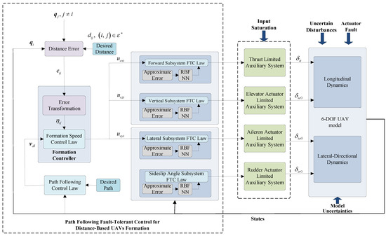
Figure 2. Fault-tolerant control structure for path following of UAV formation with input saturation.

3. Distributed Adaptive Fault-Tolerant Controller Design and Analysis

3.1. Path-Following Controller of Leader UAV

In this subsection, by using the adaptive dynamic surface technology, the path tracking controller of the leader UAV is designed to achieve the tracking control. The expected path of the leader is defined as ${\mathit{p}}_{\mathit{d}}\left({\theta }_i\left(\mathrm{t}\right))=[x_{di}\right({\theta }_i),y_{di}\left({\theta }_i),h_{di}\right({\theta }_i{\left)\right]}^T\in {\mathit{R}}^3$, and the virtual arc length is parameterized ${\theta }_i\in [0;{\theta }_{fi}]$, where ${\theta }_{fi}$ is the virtual total arc length. The goal of the path tracking control is to design a tracking controller to converge the UAV position ${\mathit{p}}_i\left(t)=[x_i\right(t), y_i\left(t), h_i\right(t{\left)\right]}^T\in {\mathit{R}}^3$ to the desired path ${\mathit{p}}_{di}\left({\theta }_i\right)$. It is worth noting that the expected path ${\theta }_i$ is independent of time through the description of the path by parameters, and then the tracking problem is transformed into a static path tracking problem emphasizing geometric position.

The tracking error is defined as follows:

$${\mathit{s}}_1{}_i={\mathit{p}}_i-{\mathit{p}}_{di}$$

(16)

$${\zeta }_i={\dot{\theta }}_i-v_{d_i}({\theta }_i)$$

(17)

where ${\mathit{s}}_{1i}$ represents the position tracking error and ${\mathit{\zeta }}_i$ represents the path parameter velocity tracking error.

Taking the derivative of ${\mathit{s}}_{1i}$ and ${\mathit{\zeta }}_i$, we have

$${\dot{\mathit{s}}}_{1i}={\mathit{v}}_i-{\mathit{p}}_{\mathit{d}i}^{{\theta }_i}({\mathit{v}}_{di}+{\mathit{\zeta }}_i)$$

(18)

$${\mathit{p}}_{{\mathit{d}}_i}^{{\theta }_i}=\partial {\mathit{p}}_{\mathit{d}i}^{}/\partial {\theta }_i$$

(19)

We choose the following Lyapunov function

$$L_1=\frac{1}{2}{\mathit{s}}_1^T{\mathit{s}}_1+\frac{1}{2k_1{k}_2}{\zeta }^2$$

(20)

where $k_1,k_2$ are the subfunction gain.

From (18) and (19), the time derivative of (20) is

$$\begin{array}{c}{\dot{L}}_1={\mathit{s}}_1{}^T\mathit{v}-{\mathit{s}}_1{}^T{\mathit{p}}_d^{\theta }(v_d+\zeta )+\frac{1}{k_1{k}_2}\zeta (\ddot{\theta }-v_d^{\theta }\dot{\theta }(t))\\ ={\mathit{s}}_1{}^T(\mathit{v}-{\mathit{p}}_d^{\theta }{\mathit{v}}_d)+\zeta (\frac{1}{k_1{k}_2}\ddot{\theta }-\frac{1}{k_1{k}_2}{v}_d^{\theta }\dot{\theta }(t)-{\mathit{s}}_1{}^T{\mathit{p}}_d^{\theta })\end{array}$$

(21)

The feedback control law of the leader is designed as

$$v_{dl}=-{\mathit{K}}_1{\mathit{e}}_{\mathit{1}}+{\mathit{p}}_{\mathit{d}}^{\theta }{v}_d$$

(22)

Next, the path parameter is proposed as follows:

$$\ddot{\theta }=-k_1\zeta +k_1{k}_2{\mathit{s}}_1^T{\mathit{p}}_d^{\theta }+v_d^{\theta }\dot{\theta }(t)$$

(23)

3.2. Distance-Based Formation Controller Design of UAVs

3.2.1. Tracking Speed Control Law for UAVs

Considering the multi-UAV system in three-dimensional space, the kinematics of i-th UAV can be described as

$${\dot{q}}_i=u_i,i=1,\dots ,n$$

(24)

where $q_i\in R^3$ denotes the position in the inertial frame and $u_i\in R^3$ is the control input.

The relative position between neighboring UAVs can be designed as

$${\tilde{q}}_{ij}=q_i-q_j, \left(i, j\right)\in {\epsilon }^{\ast }$$

(25)

Thus, for each edge of the rigid graph, the distance error can be defined by

$$e_{ij}={\tilde{q}}_{ij}-d_{ij}, \left(i, j\right)\in {\epsilon }^{\ast }$$

(26)

where ${\tilde{q}}_{ij}$ is the actual distance between agents $i$ and $j$.

Assuming the minimum and infinitesimal rigidity under the initial conditions of the diagram of the formation, the control objective is to design a distributed robust control system and to satisfy

$$ℱ\left(t\right)\to Iso({ℱ}^{\ast }) as t\to \infty$$

(27)

$$-{\underset{\_}{e}}_{ij}\left(t\right)<e_{ij}\left(t\right)<{\overline{e}}_{ij}\left(t\right), \left(i, j\right)\in {\epsilon }^{\ast },\forall t\ge 0$$

(28)

where ${\underset{\_}{e}}_{ij}\left(t\right)>0$, ${\overline{e}}_{ij}\left(t\right)>0$, and $li{m}_{t\to \infty }{\underset{\_}{e}}_{ij}\left(t\right)>0$, $li{m}_{t\to \infty }{e}_{ij}\left(t\right)>0$.

If we define the square distance error as ${\eta }_{ij}=\left|\right|{\tilde{\mathit{q}}}_{ij}|{|}^{2 }-d_{ij}{}^2, \left(i, j\right)\in {\epsilon }^{\ast }$, then we can obtain

$${\eta }_{ij}=e_{ij}(|\left|{\tilde{\mathit{q}}}_{ij}\right||+d_{ij})$$

(29)

Until now, the error can be rewritten as

$$-{\underset{\_}{\eta }}_{ij}\left(t\right)<{\eta }_{ij}\left(t\right)<{\overline{\eta }}_{ij}\left(t\right), \left(i, j\right)\in {\epsilon }^{\ast }$$

(30)

where ${\overline{\eta }}_{ij}\left(t\right)={\overline{b}}_{ij}{\rho }_{ij}\left(t\right)$, ${\underset{\_}{\eta }}_{ij}\left(t\right)={\underset{\_}{b}}_{ij}{\rho }_{ij}\left(t\right)$, and ${\overline{b}}_{ij}, {\underset{\_}{b}}_{ij}>0$.

Then, we have

$${\overline{e}}_{ij}^2\left(0\right)+2d_{ij}{\overline{e}}_{ij}\left(0\right)={\overline{b}}_{ij}{\rho }_{ij0}$$

(31)

$$2d_{ij}{\underset{\_}{e}}_{ij}\left(0\right)-{\underset{\_}{e}}_{ij}^2\left(0\right)={\underset{\_}{b}}_{ij}{\rho }_{ij0}$$

(32)

From (23) and (24), the time derivative of $e_{ij}$ is

$${\dot{e}}_{ij}={\tilde{q}}_{ij}^T \left(u_i-u_j+{\delta }_i-{\delta }_j\right)/\left(e_{ij}+d_{ij}\right), \left(i, j\right)\in {\epsilon }^{\ast }$$

(33)

From (31) and (27), the derivative of ${\eta }_{ij}$ is given by

$${\dot{\eta }}_{ij}=2{\tilde{q}}_{ij}^T \left(u_i-u_j+{\delta }_i-{\delta }_j\right), \left(i, j\right)\in {\epsilon }^{\ast }$$

(34)

From the rigid graph matrix, Equation (34) can be rewritten as

$$\dot{\mathit{\eta }}=2\mathit{R}\left(\mathit{q}\right)(\mathit{u}+\mathit{\delta })$$

(35)

where $\mathit{u}=\mathrm{col}\left(u_i\right)\in R^{3n}$, $\mathit{\delta }=\mathrm{col}\left({\delta }_i\right)\in R^{3n}$, and $\mathit{\eta }=\mathrm{col}({\eta }_{ij})\in R^l,\left(i, j\right)\in {\epsilon }^{\ast }$.

The squared distance error is designed as

$${\widehat{\eta }}_{ij}\left(t\right)=\frac{{\eta }_{ij}\left(t\right)}{{\rho }_{ij}\left(t\right)}, \left(i, j\right)\in {\epsilon }^{\ast }$$

(36)

Then, the error system can be rewritten as

$${\sigma }_{ij}=T_{ij}\left({\widehat{\eta }}_{ij}\right)=\frac{1}{2}ln\left(\frac{{\overline{b}}_{ij}{\widehat{\eta }}_{ij}+{\overline{b}}_{ij}{\widehat{b}}_{ij}}{{\overline{b}}_{ij}{\underset{\_}{b}}_{ij}-{\underset{\_}{b}}_{ij}{\widehat{\eta }}_{ij}}\right), \left(i, j\right)\in {\epsilon }^{\ast }$$

(37)

Taking the time derivative of ${\sigma }_{ij}$, we have

$$\begin{array}{ll}{\dot{\sigma }}_{ij}& =\left(d{T}_{ij}/d{\widehat{\eta }}_{ij}\right){\dot{\widehat{\eta }}}_{ij}\\ & =0.5\left[1/\left({\widehat{\eta }}_{ij}+{\underset{\_}{b}}_{ij}\right)-1/\left({\widehat{\eta }}_{ij}-{\overline{b}}_{ij}\right)\right]\times \left[\left({\dot{\eta }}_{ij}/{\rho }_{ij}\right)-\left({\eta }_{ij}{\dot{\rho }}_{ij}/{\rho }_{ij}^2 \right)\right]\\ & =0.5 {\xi }_{ij}\left({\dot{\eta }}_{ij}-{\widehat{\eta }}_{ij}{\dot{\rho }}_{ij}\right)\end{array}$$

(38)

where

$${\xi }_{ij}=\frac{1}{{\rho }_{ij}}[\frac{1}{{\widehat{\eta }}_{ij}+{\underset{\_}{b}}_{ij}}-\frac{1}{{\widehat{\eta }}_{ij}-{\overline{b}}_{ij}}], \left(i, j\right)\in {\epsilon }^{\ast }$$

(39)

Then, ${\dot{\sigma }}_{ij}$ can be written as the following form

$$\dot{\mathit{\sigma }}=\frac{1}{2}\mathit{\xi }\left(\dot{\mathit{\eta }}-\dot{\mathit{\rho }}\widehat{\mathit{\eta }}\right)$$

(40)

where $\mathit{\xi }=diag({\xi }_{ij})\in R^{l\times l}$, $\widehat{\mathit{\eta }}=col\left({\widehat{\eta }}_{ij}\right)\in R^l$, and $\left(i, j\right)\in {\epsilon }^{\ast }$.

We design the following controller

$$\mathit{u}=-{\mathit{R}}^{\mathrm{T}}\mathit{\xi }\mathit{K}\mathit{\sigma }$$

(41)

where $\mathit{K}=diag\left(k_{ij}\right)>0$ and R is the rigid diagram matrix.

According to the tracking control speed $v_{dl}$ in Section 3.1, which is only available to the formation leader, we define the center position of the formation as follows:

$$q_c\left(t\right)=\left(1/n\right){\Sigma }_{i=1}^n q_i\left(t\right)=\left(1/n\right)(1_n^T\otimes I_m)q\left(t\right)$$

(42)

Thus, we define the control law ${\dot{q}}_c\left(t\right)=v_{dl}$, so that the path tracking control of the UAV formation in three-dimensional space can be realized.

The tracking speed control law $u_{c }={[u_{cx },u_{cy },u_{cz }]}^T$ is designed as

$$u_{\mathrm{c} }=-R\xi K\sigma +n{M}_L{v}_{dl}\left(t\right)$$

(43)

where $M_L\in R^{mn\times m}$.

For each edge of the graph, we choose a Lyapunov function candidate:

$$L_{ij}=0.5 k_{ij}{\sigma }_{ij}^2 , \left(i, j\right)\in {\epsilon }^{\ast }$$

(44)

Considering the entire graph system, from (44), the Lyapunov function is defined as

$$L_2={\displaystyle \sum _{\left(i,j\right)\in {\epsilon }^{\ast }}{L}_{ij}({\sigma }_{ij})=0.5{\sigma }^{\mathrm{T}}K\sigma }$$

(45)

Taking the time derivative of $L_2$ gives

$${\dot{L}}_2={\sigma }^{T}K\xi Ru+{\sigma }^{T}K\xi R\delta -0.5{\sigma }^{T}K\xi \dot{\rho }\widehat{\eta }$$

(46)

3.2.2. PPC Design for Longitudinal Dynamics

In this section, it will be shown that the longitudinal fault-tolerant tracking controller is designed based on the backstepping method. The vertical controller system includes a forward motion subsystem and a vertical motion subsystem. In order to achieve the objective of this section, the neural network controller is used to compensate for external uncertain perturbations and the adaptive sliding mode controller is used to achieve fault-tolerant control with actuator failures. An auxiliary controller considering input constraints is used to compensate for the nonlinear characteristics of control input saturation.

(a) Forward subsystem

According to the $u_{cix}$ designed in Section 3.2.1, the desired flight speed can be obtained from (6a).

$$V_{id}=\frac{u_{cix}}{g_{ix}}$$

(47)

To avoid the differential explosion phenomenon caused by derivatives, the controller is designed using the dynamic surface method and a first-order filter is introduced as

$${\tau }_{i1}{\dot{V}}_{id}+V_{id}={\overline{V}}_{id},V_{id}(0)={\overline{V}}_{id}(0)$$

(48)

where $V_{id}$ is a virtual control signal and ${\tau }_{i1}$ is time constant.

We define the first-order filter error as ${\zeta }_{i1}=V_{id}-{\overline{V}}_{id}$, and the time derivative of ${\zeta }_{i1}$ is

$${\dot{\zeta }}_{i1}={\dot{V}}_{id}-{\dot{\overline{V}}}_{id}=\frac{{\overline{V}}_{id}-V_{id}}{{\tau }_{i1}}-{\dot{\overline{V}}}_{id}=-\frac{{\zeta }_{i1}}{{\tau }_{i1}}+M_{i1}$$

(49)

where $M_{i1}=-{\dot{\overline{V}}}_{id}$.

We define the speed tracking error as

$$s_{i1}=V_i-{\overline{V}}_{id}$$

(50)

The time derivative of $s_1$ can be then calculated as

$${\dot{s}}_{i1}=f_{iv}+g_{iv}{\delta }_{it}+d_{i1}-{\overline{V}}_{id}$$

(51)

Consider the following Lyapunov function:

$$L_{i1}=\frac{1}{2}{s}_{i1}^2+\frac{1}{2}{\zeta }_{i1}^2$$

(52)

The time derivative of (52) is

$${\dot{L}}_{i1}=s_{i1}(f_{iv}+g_{iv}{\delta }_{it}+d_{i1}-{\overline{V}}_{id})-\frac{{\zeta }_{i1}^2}{{\tau }_{i1}}+{\zeta }_{i1}{M}_{i1}$$

(53)

We propose the following thrust control input:

$${\delta }_{it}=g_{i1}^{-1}(-f_{i1}(\cdot )+{\dot{V}}_{id}-k_{i1}{s}_{i1})$$

(54)

where if $f_{i1}(\cdot )=f_{iv}+d_{i1}$ and $f_{i1}$ is an unknown nonlinear vector, then the radial basis function neural network (RBFNN) is used to estimate $f_{i1}(\cdot )$, which is given by

$$f_{i1}(\cdot )=W_{i1}^{T}h({\xi }_{i1})+{\epsilon }_{i1}$$

(55)

where ${\xi }_{i1}$ and $W_{i1}$ are the input and optimal weighting vector of RBFNN, ${\epsilon }_{i1}$ is the estimation error, which satisfies ${\epsilon }_{i1}\le \left|{\epsilon }_M\right|$, and ${\epsilon }_M>0$ is a constant. The control law is expressed as

$${\delta }_{it}=g_{i1}^{-1}(-{\widehat{W}}_{i1}^{T}h({\xi }_{i1})+{\dot{V}}_{id}-k_{i1}{s}_{i1})$$

(56)

where ${\widehat{W}}_{i1}$ represents the estimation of $W_{i1}$.

We design the adaptive law as

$${\dot{\widehat{W}}}_{i1}={\mathrm{\Gamma }}_{i1}[-h({\xi }_{i1})s_{i1}^T-k_{Wi1}{\widehat{W}}_{i1}]$$

(57)

where ${\mathrm{\Gamma }}_{i1}>0$ and $k_{Wi1}>0$ are constants.

The approximation error of RBFNN is ${\tilde{W}}_{i1}^T={\widehat{W}}_{i1}^T-W_{i1}^T$.

In order to solve the input saturation problem of UAV engine thrusts in the actual flight control process, the auxiliary system is designed as

$${\dot{w}}_{i1}=\{\begin{array}{l}-k_{wi1}{w}_{i1}-\frac{f_{1i}}{{\Vert w_i\Vert }^2}+k_{\delta i1}\mathrm{\Delta }{\delta }_{it},\Vert w_i\Vert \ge w_0\\ 0,\hspace{1em}\hspace{1em}\hspace{1em}\hspace{1em}\hspace{1em}\hspace{1em}\hspace{1em}\hspace{1em}\hspace{1em}\hspace{1em}\Vert w_i\Vert <w_0\end{array}$$

(58)

where $f_{1i}=(\left|s_{i1}\mathrm{\Delta }{\delta }_{it}\right|+0.5{\delta }_{it}^2)w_i$ and $\mathrm{\Delta }{\delta }_{it}={\delta }_{it}-{\delta }_{cit}$. And $w_{i1}\in R$ represents the state variable for the auxiliary system. $k_{wi1}$, $k_{\delta i1}$, and $w_0$ are constants to be designed. ${\delta }_{it}$ and ${\delta }_{cit}$ represent the actual control input and the desired control input, respectively. The auxiliary system is adjusted when input saturation occurs in the system, such as when the input saturation is eliminated, $\mathrm{\Delta }{\delta }_{it}=0$, ${\dot{w}}_{i1}=-k_{wi1}{w}_{i1}$, and $w_{i1}$ decay exponentially to $\Vert w_{i1}\Vert <w_0$ until ${\dot{w}}_{i1}=0$; otherwise, when saturation occurs again, $\Vert w_{i1}\Vert \ge w_0$, the auxiliary system will be adjusted again.

Considering the errors of RBFNN and the auxiliary system, we choose the following Lyapunov function

$$L_{i2}=L_{i1}+\frac{1}{2}tr({\tilde{W}}_{i1}{\mathrm{\Gamma }}_{i1}^{-1}{\tilde{W}}_{i1})+\frac{1}{2}{w}_{i1}^2$$

(59)

Differentiating (59) yields

$${\dot{L}}_{i2}=-k_{i1}{s}_{i1}^2-k_{Wi1}tr({\tilde{W}}_{i1}^T{\tilde{W}}_{i1})-\frac{1}{2}\frac{{\zeta }_{i1}^2}{{\tau }_{i1}}+{\zeta }_{i1}{M}_{i1}-w_{i1}(k_{wi1}-0.5k_{i2})w_{i1}$$

(60)

(b) Vertical subsystem

Based on the $u_{ciz}$ in Section 3.2.1, the desired trajectory angle is obtained from (6a).

$${\gamma }_{id}=-V_i^{-1}{u}_{ciz}$$

(61)

We define $s_{i2}={\gamma }_i-{\gamma }_{id}$, and the time derivative of $s_{i2}$ is

$${\dot{s}}_{i2}=f_{i\gamma }+g_{i\gamma }{\theta }_i+d_{i2}-{\dot{\gamma }}_{id}$$

(62)

We define the Lyapunov function as

$$L_{i3}=\frac{1}{2}{s}_{i2}^2$$

(63)

The time derivative of (63) is

$${\dot{L}}_{i3}=s_{i2}(f_{i\gamma }+g_{i\gamma }+d_{i2}-{\dot{\gamma }}_{id})$$

(64)

We design the pitch angle control input as

$${\theta }_{id}=g_{ir}^{-1}(-f_{i2}(.)+{\dot{\gamma }}_{id}-k_{i3}{s}_{i2})$$

(65)

where $f_{i2}(.)=f_{ir}+d_{i2}$. Because $f_{i2}(.)$ is an unknown nonlinear vector, the RBFNN is used to estimate $f_{i2}(.)$.

$$f_{i2}(.)=W_{i2}^{T}h\left({\xi }_{i2}\right)+{\epsilon }_{i2}$$

(66)

where ${\xi }_{i2}$ and $W_{i2}^{}$ are the input and optimal weighting vector of RBFNN and ${\epsilon }_{i2}$ is the estimation error, which satisfies ${\epsilon }_{i2}\le \left|{\epsilon }_M\right|$. We define the pitch angle control input as

$${\theta }_{id}=g_{ir}^{-1}(-{\widehat{W}}_{i2}^{T}h\left({\xi }_{i2}\right)+{\dot{\gamma }}_{id}-k_{i3}{s}_{i2})$$

(67)

where ${\widehat{W}}_{i2}^T$ is the estimation of ${\widehat{W}}_{i2}$. We design the adaptive law as

$${\dot{\widehat{W}}}_{i2}={\mathrm{\Gamma }}_{i2}[-h({\xi }_{i2})s_{i2}^T-k_{Wi2}{\widehat{W}}_{i2}]$$

(68)

where ${\mathrm{\Gamma }}_{i2}\in R$ and $k_{Wi2}\in R$ are constants.

The approximation error of RBFNN is ${\tilde{W}}_{i2}^T={\widehat{W}}_{i2}^T-W_{i2}^T$. The first-order filter is introduced to compute the time derivative of the control signal, which is designed as

$${\tau }_{i2}{\dot{\theta }}_{id}+{\theta }_{id}={\overline{\theta }}_{id},{\theta }_{id}(0)={\overline{\theta }}_{id}(0)$$

(69)

where ${\overline{\theta }}_{id}$ is the virtual control signal and ${\tau }_{i2}>0$ is a time constant.

We define the first-order filter error as ${\zeta }_{i2}={\theta }_{id}-{\overline{\theta }}_{id}$, and the time derivative of ${\zeta }_{i2}$ is

$${\dot{\zeta }}_{i2}={\dot{\theta }}_{id}-{\dot{\overline{\theta }}}_{id}=\frac{{\dot{\theta }}_{id}-{\dot{\overline{\theta }}}_{id}}{{\tau }_{i2}}-{\dot{\overline{\theta }}}_{id}=-\frac{{\zeta }_{i2}}{{\tau }_{i2}}+M_{i2}$$

(70)

where $M_{i2}=-{\dot{\overline{\theta }}}_{id}$.

We define the Lyapunov function as

$$L_{i4}=L_{i3}+\frac{1}{2}tr({\tilde{W}}_{i2}^T{\mathrm{\Gamma }}_{i2}^{-1}{\tilde{W}}_{i2})+\frac{1}{2}{\zeta }_{i2}^2$$

(71)

The time derivative of (71) is

$${\dot{L}}_{i4}=-k_{i3}{s}_{i2}^2-k_{W_{i2}}tr({\tilde{W}}_{i2}^T{\tilde{W}}_{i2})-\frac{1}{2}\frac{{\zeta }_{i2}^2}{{\tau }_{i2}}+{\zeta }_{i2}{M}_{i2}$$

(72)

By defining the pitch angle tracking error $s_{i3}={\theta }_i-{\theta }_{id}$, one has ${\dot{s}}_{i3}={\dot{\theta }}_i-{\dot{\theta }}_{id}=q_i-{\dot{\theta }}_{id}$.

The pitch angle rate control signal is designed as

$$q_{id}=-k_{i4}{S}_{i3}+{\dot{\theta }}_{id}$$

(73)

where $k_{i4}>0$ is a constant. The first-order filter is introduced as

$${\tau }_{i3}{\dot{q}}_{id}+q_{id}={\overline{q}}_{id}, q_{id}(0)={\overline{q}}_{id}(0)$$

(74)

where ${\overline{q}}_{id}$ is the virtual control signal and ${\tau }_{i3}$ is the time constant.

Define the first-order filter error as ${\zeta }_{i3}=q_{id}-{\overline{q}}_{id}$, and the time derivative of ${\zeta }_{i3}$ is

$${\dot{\zeta }}_{i3}={\dot{q}}_{id}-{\dot{\overline{q}}}_{id}=\frac{{\overline{q}}_{id-}{q}_{id}}{{\tau }_{i3}}-{\dot{\overline{q}}}_{id}=-\frac{{\zeta }_{i3}}{{\tau }_{i3}}+M_{i3}$$

(75)

where $M_{i3}=-{\dot{\overline{q}}}_{id}$.

We choose the Lyapunov function

$$L_{i5}=L_{i4}+\frac{1}{2}{s}_{i3}^2+\frac{1}{2}{\zeta }_{i3}^2$$

(76)

The time derivative of (76) is

$${\dot{L}}_{i5}=-k_{i3}{s}_{i2}^2-k_{i4}{s}_{i3}^2-k_{Wi2}tr({\tilde{W}}_{i2}^T{\tilde{W}}_{i2})-\frac{1}{2}\frac{{\zeta }_{i2}^2}{{\tau }_{i2}}-\frac{1}{2}\frac{{\zeta }_{i3}^2}{{\tau }_{i3}}+{\zeta }_{i2}{M}_{i2}+{\zeta }_{i3}{M}_{i3}$$

(77)

If we define the pitch angle rate tracking error as $s_{i4}=q_i-q_{id}$, then one has

$${\dot{s}}_{i4}={\dot{q}}_i-{\dot{q}}_{id}=f_{iq}+g_{iq}{\rho }_{ife}{\delta }_{ie0}+d_{i30}-{\dot{q}}_{id}$$

(78)

Then, the elevator control input signal is designed as

$${\delta }_{ie0}=g_{{}_{iq}}^{-1}{\rho }_{ife}^{-1}(f_{i3}(\cdot )+{\dot{q}}_{id}-k_{i5}{s}_{i4})$$

(79)

where $f_{i3}(\cdot )=f_{iq}+d_{i30}$.

The RBFNN is used to estimate $f_{i3}(\cdot )$, which is given by

$$f_{i3}(\cdot )=W_{i3}^{T}h({\zeta }_{i3})+{\epsilon }_{i3}$$

(80)

where ${\zeta }_{i3}$ and $W_{i3}$ are the input and optimal weighting vector of RBFNN and ${\epsilon }_{i3}$ is the estimation error, which satisfies ${\epsilon }_{i3}\le \left|{\epsilon }_M\right|$.

Based on (80), the adaptive law is designed as

$${\dot{\widehat{W}}}_{i3}={\mathrm{\Gamma }}_{i3}[-h({\xi }_{i3})s_{i4}^T-k_{Wi3}{\widehat{W}}_{i3}]$$

(81)

where ${\widehat{W}}_{i3}$ is estimation of $W_{i3}$ and ${\tilde{W}}_{i3}^T={\widehat{W}}_{i3}^T-W_{i3}^T$ is the approximation error of RBFNN.

By introducing the adaptive sliding mode function to realize the fault-tolerance control for the unknown faults of an elevator actuator, the sliding mode function is designed as

$$S_{i1}=c_{i1}{s}_{i3}+{\dot{s}}_{i3}$$

(82)

where $c_{i1}>0$ is a constant and the time derivative of (82) is

$$\begin{array}{l}{\dot{S}}_{i1}=c_{i1}{\dot{s}}_{i3}+{\ddot{s}}_{i3}=c_{i1}{\dot{s}}_{i3}+{\dot{q}}_i-{\ddot{\theta }}_d\\ {=}_{i1}{\dot{s}}_{i3}+f_{iq}{\rho }_{ifq}{\delta }_{ie0}+f_{i3}-{\ddot{\theta }}_d\end{array}$$

(83)

Taking ${\lambda }_{i1}=f_{iq}{\rho }_{ifq}$ and ${\varpi }_{i1}=\frac{1}{{\lambda }_{i1}}$, we choose the following Lyapunov function

$$L_{i6}=\frac{1}{2}{S}_{i1}^2+\frac{\left|{\lambda }_{i1}\right|}{2{\kappa }_{i1}}{\tilde{\varpi }}_{i1}^2+\frac{1}{2}tr({\tilde{W}}_{i3}^T{\mathrm{\Gamma }}^{-1}{\tilde{W}}_{i3})$$

(84)

where ${\tilde{\varpi }}_{i1}={\widehat{\varpi }}_{i1}-{\varpi }_{i1},{\kappa }_{i1}>0$. The time derivative of (84) is

$$\begin{array}{l}{\dot{L}}_{i6}=S_{i1}{\dot{S}}_{i1}+\frac{\left|{\lambda }_{i1}\right|}{{\kappa }_{i1}}{\tilde{\varpi }}_{i1}{\dot{\tilde{\varpi }}}_{i1}-k_{Wi3}tr({\tilde{W}}_{i3}^T{\tilde{W}}_{i3})=S_{i1}[c_{i1}{\dot{s}}_{i2}+{\lambda }_{i1}{\delta }_{ie0}+f_{i2}-{\ddot{\psi }}_{id}]\\ \hspace{1em}\hspace{1em}+\frac{\left|{\lambda }_{i1}\right|}{{\kappa }_{i1}}{\tilde{\varpi }}_{i1}{\dot{\tilde{\varpi }}}_{i1}-k_{Wi3}tr({\tilde{W}}_{i3}^T{\tilde{W}}_{i3})\end{array}$$

(85)

We design the virtual control signal as

$${\alpha }_{i1}=k_{i4}{S}_{i1}+c_{i1}{s}_{i2}+f_{i3}-{\ddot{\theta }}_{id}-{\eta }_{i1}\mathrm{sgn}{S}_{i1}$$

(86)

where $k_{i4}>0$ and ${\eta }_{i1}\ge {\epsilon }_M$.

Substituting (85) into (84) gives

$$\begin{array}{l}{\dot{L}}_{i6}=S_{i1}[{\alpha }_{i1}-k_{i4}{S}_{i1}+{\lambda }_{i1}{\delta }_{ie0}+{\tilde{f}}_{i1}]+\frac{\left|{\lambda }_{i1}\right|}{{\kappa }_{i1}}{\tilde{\varpi }}_{i1}{\dot{\widehat{\varpi }}}_{i1}-k_{Wi3}tr({\tilde{W}}_{i3}^T{\tilde{W}}_{i3})\\ \hspace{1em}=S_{i1}[{\alpha }_{i1}-k_{i4}{S}_{i1}+{\lambda }_{i1}{\delta }_{ie0}+W_{i3}h({\xi }_{i3})+{\epsilon }_{i3}]+\frac{\left|{\lambda }_{i1}\right|}{{\kappa }_{i1}}{\tilde{\varpi }}_{i1}{\dot{\widehat{\varpi }}}_{i1}-k_{Wi3}tr({\tilde{W}}_{i3}^T{\tilde{W}}_{i3})\\ \hspace{1em}=S_{i1}[{\alpha }_{i1}-k_{i4}{S}_{i1}+{\lambda }_{i1}{\delta }_{ie0}+{\epsilon }_{i2}]+\frac{\left|{\lambda }_{i1}\right|}{{\kappa }_{i1}}{\tilde{\varpi }}_{i1}{\dot{\widehat{\varpi }}}_{i1}-k_{Wi3}tr({\tilde{W}}_{i3}^T{\tilde{W}}_{i3})\end{array}$$

(87)

We design control law and adaptive law as

$${\delta }_{ie0}=-{\widehat{\varpi }}_{i1}{\alpha }_{i1}$$

(88)

$${\widehat{\varpi }}_{i1}={\kappa }_{i1}{S}_{i1}{\alpha }_{i1}\mathrm{sgn}{g}_{iq}$$

(89)

where $\mathrm{sgn}{g}_{iq}=\mathrm{sgn}{\lambda }_{i1}$.

Considering the elevator control input saturation of the UAV during the actual flight control process, the following auxiliary system is designed as

$${\dot{w}}_{i2}=\{\begin{array}{c}-k_{wi2}{w}_{i2}-\frac{f_{2i}}{{\Vert w_{i2}\Vert }^2}+k_{\delta i2}\mathrm{\Delta }{\delta }_{ie},\Vert w_{i2}\Vert \ge w_0\\ 0,\hspace{1em}\Vert w_{i2}\Vert <w_0\hspace{1em}\hspace{1em}\hspace{1em}\hspace{1em}\end{array}$$

(90)

where $f_{2i}=(|s_{i3}\mathrm{\Delta }{\delta }_{ie}|+0.5{\delta }_{ie}^2)w_i$ and $\mathrm{\Delta }{\delta }_{ie}={\delta }_{ie}-{\delta }_{cie}$. $w_{i2}\in R$ is the state variable of the auxiliary system, $k_{wi2}$, $k_{\delta i2}$, and $w_0$ are constants to be designed, and ${\delta }_{ie}1$ and ${\delta }_{cie}$ are the actual control input and the desired control input.

Considering the influence of the pitch angle rate tracking errors and auxiliary control systems, we choose the following Lyapunov function

$$L_{i7}=\frac{1}{2}{s}_{i4}^2+\frac{1}{2}{w}_{i2}^2$$

(91)

The time derivative of (91) is

$${\dot{L}}_{i7}=-k_{i5}{s}_{i4}^2-w_{i2}(k_{wi2}-0.5k_{i6})w_{i2}$$

(92)

3.2.3. The Transverse Lateral Controller Design of the Drone under Restricted Conditions

This subsection will design the lateral and lateral fault-tolerant controller of the UAV according to Section 3.2.1 and Section 3.2.2 and will design the distributed fault-tolerant controller for the lateral control subsystem and the lateral slip angle control subsystem with an aileron actuator failure and a rudder actuator failure, respectively, by the dynamic surface neural network control technique.

(a) Lateral subsystem

According to the $u_{ciy}$ designed in Section 3.2.1, the desired yaw angle can be obtained as

$${\psi }_{id}=\arcsin \frac{V_i\cos {\theta }_i}{u_{ciy}}$$

(93)

To avoid the differential explosion phenomenon caused by derivatives, the first-order filter is designed as

$${\tau }_{i4}{\dot{\psi }}_{id}+{\psi }_{id}={\overline{\psi }}_{id},{\psi }_{id}(0)={\overline{\psi }}_{id}(0)$$

(94)

where ${\overline{\psi }}_{id}$ is the virtual control signal and ${\tau }_{i4}$ is a time constant.

By defining the filtering error as ${\zeta }_{i4}={\psi }_{id}-{\overline{\psi }}_{id}$, the time derivative of ${\zeta }_{i4}$ is

$${\dot{\zeta }}_{i4}={\dot{\psi }}_{id}-{\dot{\overline{\psi }}}_{id}=\frac{{\dot{\overline{\psi }}}_{id}-{\psi }_{id}}{{\tau }_{i4}}-{\dot{\overline{\psi }}}_{id}=-\frac{{\zeta }_{i4}}{{\tau }_{i4}}+M_{i4}$$

(95)

where $M_{i4}=-{\dot{\overline{\psi }}}_{id}$.

We define the first-order filter error as $s_{i5}={\psi }_i-{\psi }_{id}$, and the virtual control signal is designed as

$${\psi }_i=-k_{i5}{s}_{i6}+{\dot{\psi }}_{id}$$

(96)

We choose the following Lyapunov function

$$L_{i8}=\frac{1}{2}{s}_{i5}^2+\frac{1}{2}{\xi }_{i4}^2$$

(97)

The time derivative of (97) is

$${\dot{L}}_{i8}=-k_{i6}{s}_{i5}^2-\frac{1}{2}\frac{{\xi }_{i4}^2}{{\tau }_{i4}}+{\zeta }_{i4}{M}_{i4}$$

(98)

The relationship between the angular velocity $r$ and the Euler angular velocity can be expressed as

$$r_i=-{\dot{\theta }}_i\sin {\varphi }_i+{\dot{\psi }}_i\cos {\varphi }_i\cos {\theta }_i$$

(99)

In the lateral motion of UAV, we have

$${\dot{\psi }}_i=r_i\cos {\varphi }_i$$

(100)

According to (99) and (100), the expected roll angle can be expected as

$${\varphi }_{id}=\frac{1}{2}\left(\arcsin \frac{2{\dot{\psi }}_i-{\dot{\psi }}_i\cos \theta }{\sqrt{{\dot{\theta }}_i^2+{\dot{\psi }}^2{}_i{\cos }^2{\theta }_i}}-\arccos \frac{-{\dot{\theta }}_i}{\sqrt{{\dot{\theta }}_i^2+{\dot{\psi }}^2{}_i{\cos }^2{\theta }_i}}\right)$$

(101)

We define the roll angle tracking error as $s_{i6}={\varphi }_i-{\varphi }_{id}$, and the time derivative of $s_{i6}$ is

$${\dot{s}}_{i6}=f_{i\varphi }+p_i-{\dot{\varphi }}_{id}$$

(102)

The roll angle rate is designed as

$$p_{id}=-k_{i7}{s}_{i6}-f_{i\varphi }+{\dot{\varphi }}_{id}$$

(103)

where $k_{i7}>0$ is the parameter to be designed.

The first-order filter is constructed as

$${\tau }_{i5}{\dot{p}}_{id}+p_{id}={\overline{p}}_{id},\hspace{0.17em}{p}_{id}(0)={\overline{p}}_{id}(0)$$

(104)

where ${\overline{p}}_{id}$ is a virtual control signal and ${\tau }_{i5}$ is time constant.

We define the filtering error as ${\zeta }_{i5}=p_{id}-{\overline{p}}_{id}$, and the time derivative of ${\zeta }_{i5}$ is

$${\dot{\zeta }}_{i5}={\dot{p}}_{id}-{\dot{\overline{p}}}_{id}=\frac{{\overline{p}}_{id}-p_{id}}{{\tau }_{i5}}-{\dot{\overline{p}}}_{id}=-\frac{{\zeta }_{i5}}{{\tau }_{i5}}+M_{i5}$$

(105)

where $M_{i5}=-{\dot{\overline{p}}}_{id}$.

We choose the following Lyapunov function

$$L_{i9}=L_{i8}+\frac{1}{2}{s}_{i6}^2+\frac{1}{2}{\xi }_{i5}^2$$

(106)

The time derivative of (106) is

$${\dot{L}}_{i9}=-k_{i6}{s}_{i5}^2-k_{i7}{s}_{i6}^2-\frac{1}{2}\frac{{\zeta }_{i4}^2}{{\tau }_{i4}}-\frac{1}{2}\frac{{\zeta }_{i5}^2}{{\tau }_{i5}}+{\zeta }_{i4}{M}_{i4}+{\zeta }_{i5}{M}_{i5}$$

(107)

If we define the roll angle rate tracking error as

$$s_{i7}=p_i-p_{id}$$

(108)

then one has

$$\begin{array}{l}{\dot{s}}_{i7}={\dot{p}}_i-{\dot{p}}_{id}\\ \hspace{1em}=f_{ip}+g_{ip}{\delta }_{iao}+d_{i40}-p_{id}\end{array}$$

(109)

We design the aileron control input signals as

$${\delta }_{iao}=g_{ip}^{-1}{\rho }_{ifa}^{-1}(f_{i4}(\cdot )+{\dot{p}}_{id}-k_{i8}{s}_{i7})$$

(110)

where $f_{i4}(\cdot )=f_{id}+d_{i40}$. The RBFNN is used to estimate $f_{i4}(.)$, which is given by

$$f_{i4}(.)=W_{i4}^{T}h({\xi }_{i4})+{\epsilon }_{i4}$$

(111)

where ${\xi }_{i4}$ and $W_{i4}$ are the input and optimal weighting vector of RBFNN and ${\epsilon }_{i4}$ is an estimation error, which satisfies ${\epsilon }_{i4}\le \left|{\epsilon }_M\right|$. The neural network output is ${\widehat{f}}_{i4}={\widehat{W}}_{i4}^{T}h({\xi }_{i4})$, and ${\widehat{W}}_{i4}$ is the estimation of $W_{i4}$. The adaptive law is designed as

$${\dot{\widehat{W}}}_{i4}={\mathrm{\Gamma }}_{i4}[-h({\xi }_{i4})s_{7i}^T-k_{wi4}{\widehat{W}}_{i4}]$$

(112)

where ${\mathrm{\Gamma }}_{i4}\in R,-k_{wi4}\in R$ are constants. The error of RBFNN is ${\tilde{W}}_{i4}^T={\widehat{W}}_{i4}^T-W_{i4}^T$.

To realize the fault-tolerance control of the aileron actuator, we introduce the following adaptive sliding mode function:

$$S_{i2}=c_{i2}{s}_{i6}+{\dot{s}}_{i6}$$

(113)

where $c_{i2}>0$ is a constant. By differentiating (112), one can obtain

$$\begin{array}{l}{\dot{S}}_{i2}=c_{i2}{\dot{s}}_{i6}+{\ddot{s}}_{i6}=c_{i2}{\dot{s}}_{i6}+{\dot{p}}_i-{\ddot{\varphi }}_{id}\\ \hspace{1em}=c_{i2}{\dot{s}}_{i6}+f_{ip}{\rho }_{ifa}{\delta }_{ia0}+f_{i4}-{\ddot{\varphi }}_{id}\end{array}$$

(114)

By defining ${\lambda }_{i2}=f_{ip}{\rho }_{ifa}$ and ${\varpi }_{i2}=\frac{1}{{\lambda }_{i2}}$, we choose the following Lyapunov function

$$L_{i10}=\frac{1}{2}{S}_{i2}^2+\frac{\left|{\lambda }_{i2}\right|}{2{\kappa }_{i2}}{\tilde{\varpi }}_{i2}^2+\frac{1}{2}tr({\tilde{W}}_{i4}^T{\mathrm{\Gamma }}_{i4}^{-1}{\tilde{W}}_{i4})$$

(115)

where ${\tilde{\varpi }}_{i2}={\widehat{\varpi }}_{i2}-{\tilde{\varpi }}_{i2},{\kappa }_{i2}>0$, and one has

$$\begin{array}{l}{\dot{L}}_{i10}=S_{i2}{\dot{S}}_{i2}+\frac{\left|{\lambda }_{i2}\right|}{{\kappa }_{i2}}{\tilde{\varpi }}_{i2}{\dot{\widehat{\varpi }}}_{i2}-k_{Wi4}tr({\tilde{W}}_{i4}^T{\tilde{W}}_{i4})\\ \hspace{1em}\hspace{1em}=S_{i2}[c_{i2}{\dot{s}}_{i6}+{\lambda }_{i2}{\delta }_{ia0}+f_{i4}-{\ddot{\varphi }}_{id}]+\frac{\left|{\lambda }_{i2}\right|}{{\kappa }_{i2}}{\tilde{\varpi }}_{i2}{\dot{\widehat{\varpi }}}_{i2}-k_{Wi4}tr({\tilde{W}}_{i4}^T{\tilde{W}}_{i4})\end{array}$$

(116)

We design the virtual control amount as

$${\alpha }_{i2}=k_{i9}{S}_{i2}+c_{i2}{S}_{i6}+f_{i4}-{\ddot{\varphi }}_{id}-{\eta }_{i2}\mathrm{sgn}{S}_{i2}$$

(117)

where $k_{i9}>0$ and ${\eta }_{i2}>{\epsilon }_M$.

Then, one has

$$\begin{array}{l}{\dot{L}}_{i10}=S_{i2}[{\alpha }_{i2}-k_{i9}{S}_{i2}+{\lambda }_{i2}{\delta }_{ia0}+{\tilde{f}}_{i4}]+\frac{\left|{\lambda }_{i2}\right|}{{\kappa }_{i2}}{\tilde{\varpi }}_{i2}{\dot{\widehat{\varpi }}}_{i2}-k_{Wi4}tr({\tilde{W}}_{i4}^T{\tilde{W}}_{i4})\\ \hspace{1em}\hspace{1em}=S_{i2}[{\alpha }_{i2}-k_{i9}{S}_{i2}+{\lambda }_{i2}{\delta }_{ia0}+{\epsilon }_{i4}]+\frac{\left|{\lambda }_{i2}\right|}{{\kappa }_{i2}}{\tilde{\varpi }}_{i2}{\dot{\widehat{\varpi }}}_{i2}-k_{Wi4}tr({\tilde{W}}_{i4}^T{\tilde{W}}_{i4})\\ \hspace{1em}=S_{i2}[{\alpha }_{i2}-k_{i9}{S}_{i2}+{\lambda }_{i2}{\delta }_{ia0}+{\tilde{f}}_{i4}+W_{i4}h({\xi }_{i4})+{\epsilon }_{i4}]+\frac{\left|{\lambda }_{i2}\right|}{{\kappa }_{i2}}{\tilde{\varpi }}_{i2}{\dot{\widehat{\varpi }}}_{i2}-k_{Wi4}tr({\tilde{W}}_{i4}^T{\tilde{W}}_{i4})\end{array}$$

(118)

We design the control law and the adaptive law as

$${\delta }_{ia0}=-{\widehat{\varpi }}_{i2}{\alpha }_{i2}$$

(119)

$$\dot{\widehat{\varpi }}={\kappa }_{i2}{S}_{i2}{\alpha }_{i2}\mathrm{sgn}{g}_{ip}$$

(120)

where $\mathrm{sgn}{g}_{ip}=\mathrm{sgn}{\lambda }_{i2}$.

In order to solve the control input saturation problem of the aileron actuator during the actual flight control of UAVs, the following auxiliary system is designed as

$${\dot{w}}_{i3}=\{\begin{array}{c}-k_{wi3}{w}_{i3}-\frac{f_{3i}}{{\Vert w_{i3}\Vert }^2}+k_{\delta i3}\mathrm{\Delta }{\delta }_{ia},\Vert w_{i3}\Vert \ge w_0\\ 0,\hspace{1em}\hspace{1em}\Vert w_{i3}\Vert <w_0\end{array}$$

(121)

where $f_{3i}=(|s_{i7}\mathrm{\Delta }{\delta }_{ia}|+0.5{\delta }_{ia}^2)w_{i3}$, $\mathrm{\Delta }{\delta }_{ia}={\delta }_{ia}-{\delta }_{cia}$, $w_{i3}\in R$ is the state variable for the auxiliary system, $k_{wi3}$, $k_{\delta i3}$, and $w_0$ are constants to be designed, and ${\delta }_{ia}$ and ${\delta }_{cia}$ are the actual control input and the desired control input.

Considering the rolling angle rate tracking error and the influence of the auxiliary control system, we choose the following Lyapunov function

$$L_{i11}=\frac{1}{2}{s}_{i7}^2+\frac{1}{2}{w}_{i3}^2$$

(122)

Taking the time derivatives of (122) yields

$${\dot{L}}_{i11}=-k_{i8}{s}_{i7}^2-w_{i3}(k_{wi3}-0.5k_{i10})w_{i3}$$

(123)

(b) Sliding angle subsystem

If we define the slip angle tracking error as $s_{i8}={\beta }_i$, then one has

$${\dot{\beta }}_i=f_{i\beta }-r_i$$

(124)

We design the yaw angle rate control input signal as

$$r_i=f_{i\beta }-k_{i11}{s}_{i8}$$

(125)

The RBFNN is used to estimate $f_{i\beta }$, which is given by

$$f_{i\beta }=W_{i5}^{T}h\left({\xi }_{i5}\right)+{\epsilon }_{i5}$$

(126)

where ${\xi }_{i5}$ and $W_{i5}$ are the input and optimal weight vector of RBFNN and ${\epsilon }_{i5}$ is the estimation error, which satisfies ${\epsilon }_{i5}\le \left|{\epsilon }_M\right|$. We define the yaw angle rate control input as

$$r_{id}={\widehat{W}}_{i5}^{T}h\left({\xi }_{i5}\right)-k_{i11}{s}_{i8}$$

(127)

The adaptive law is given by

$${\dot{\widehat{W}}}_{i5}^T={\mathrm{\Gamma }}_{i5}[-h\left({\xi }_{i5}\right)s_{i8}-k_{iW5}{\widehat{W}}_{i5}]$$

(128)

where ${\mathrm{\Gamma }}_{i5}$ and $k_{iW5}$ are constants.

The neural network approximation error is ${\tilde{W}}_{i5}^T={\widehat{W}}_{i5}^T-W_{i5}^T$. The first-order filter is introduced as

$${\tau }_{i6}{\dot{r}}_{id}+r_{id}={\overline{r}}_{id},r_{id}(0)={\overline{r}}_{id}(0)$$

(129)

where ${\overline{r}}_{id}$ is a virtual control signal and ${\tau }_{i6}$ is the time constant.

If we define the filtering error as ${\zeta }_{i6}=r_{id}-{\overline{r}}_{id}$, then one has

$${\dot{\zeta }}_{i6}={\dot{r}}_{id}-{\dot{\overline{r}}}_{id}=\frac{{\overline{r}}_{id}-{\overline{r}}_{id}}{{\tau }_{i6}}-{\dot{\overline{r}}}_{id}=-\frac{{\zeta }_{i6}}{{\tau }_{i6}}+M_{i6}$$

(130)

where $M_{i6}=-{\dot{\overline{r}}}_{id}$.

We choose the following Lyapunov function

$$L_{i12}=\frac{1}{2}{S}_{i8}^2+\frac{1}{2}{\zeta }_{i6}^2+\frac{1}{2}tr({\tilde{W}}_{i5}^T{\mathrm{\Gamma }}_{i5}^{-1}{\tilde{W}}_{i5})$$

(131)

Then, taking the time derivative of (131) yields

$${\dot{L}}_{i12}=-k_{11}{S}_{i8}^2-\frac{{\zeta }_{i6}^2}{{\tau }_{i6}}-k_{iW5}tr({\tilde{W}}_{i5}^T{\tilde{W}}_{i5})+{\zeta }_{i6}{M}_{i6}$$

(132)

If we define the yaw angle rate tracking error as $s_{i9}=r_i-r_{id}$, then one has

$${\dot{s}}_{i9}={\dot{r}}_i-{\dot{r}}_{id}=f_{ir}+g_{ir}{\delta }_{ir0}+d_{i50}-{\dot{r}}_{id}$$

(133)

We design the rudder control input signal as

$${\delta }_{ir0}=g_{ir}^{-1}{\rho }_{ifr}^{-1}(f_{i6}(\cdot )+{\dot{r}}_{id}-k_{i12}{s}_{i9})$$

(134)

where $f_{i6}(\cdot )=f_{ir}+d_{i50}$. The RBFNN is used to estimate $f_{i6}(\cdot )$, which is given by

$$f_{i6}(\cdot )=W_{i6}^{T}h({\xi }_{i6})+{\epsilon }_{i6}$$

(135)

where ${\xi }_{i6}$ and $W_{i6}$ are the input and optimal weighting vector of RBFNN and ${\epsilon }_{i6}$ is the estimation error and satisfies ${\epsilon }_{i6}\le \left|{\epsilon }_M\right|$. The neural network output is ${\widehat{f}}_{i6}={\widehat{W}}_{i6}^{T}h({\xi }_{i6})$, and the adaptive law is designed as

$${\dot{\widehat{W}}}_{i6}={\mathrm{\Gamma }}_{i6}[-h({\xi }_{i6})s_{i6}-k_{iW6}{\widehat{W}}_{i6}]$$

(136)

where ${\mathrm{\Gamma }}_{i6}\in R$ and $k_{w6}\in R$ are constants. The neural network approximation error is ${\tilde{W}}_{i6}^T={\widehat{W}}_{i6}^T-W_{i6}^T$.

In order to solve the fault-tolerant control problem of the unknown faults of a rudder actuator, the adaptive sliding mode function is introduced as

$$S_{i3}=c_{i3}{s}_{i8}+{\dot{s}}_{i8}$$

(137)

where $c_{i3}>0$.

Taking the time derivative of (136) yields

$$\begin{array}{l}{\dot{S}}_{i3}=c_{i3}{\dot{s}}_{i8}+{\ddot{s}}_{i8}=c_{i3}{\dot{s}}_{i8}+{\dot{r}}_i\\ \hspace{1em}=c_{i3}{\dot{s}}_{i8}+f_{ir}{\rho }_{ifr}{\delta }_{ir0}+f_{i6}\end{array}$$

(138)

We choose the following Lyapunov function

$$L_{i13}=\frac{1}{2}{S}_{i3}^2+\frac{\left|{\lambda }_{i3}\right|}{2{\kappa }_{i3}}{\tilde{\varpi }}_{i3}^2+\frac{1}{2}tr({\tilde{W}}_{i6}^T{\mathrm{\Gamma }}_{i6}^{-1}{\tilde{W}}_{i6})$$

(139)

where ${\tilde{\varpi }}_{i3}={\widehat{\varpi }}_{i3}-{\tilde{\varpi }}_{i3}$ and ${\kappa }_{i3}>0$. Then, we have

$$\begin{array}{l}{\dot{L}}_{i13}=S_{i3}{\dot{S}}_{i3}+\frac{\left|{\lambda }_{i3}\right|}{{\kappa }_{i3}}{\tilde{\varpi }}_{i3}{\dot{\tilde{\varpi }}}_{i3}-k_{Wi6}tr({\tilde{W}}_{i6}^T{\tilde{W}}_{i6})\\ \hspace{1em}\hspace{1em}=S_{i3}[c_{i3}{\dot{s}}_{18}+{\lambda }_{i3}{\delta }_{ir0}+f_{i6}]+\frac{\left|{\lambda }_{i3}\right|}{{\kappa }_{i3}}{\tilde{\varpi }}_{i3}{\dot{\tilde{\varpi }}}_{i3}-k_{Wi6}tr({\tilde{W}}_{i6}^T{\tilde{W}}_{i6})\end{array}$$

(140)

We design the virtual control signal as

$${\alpha }_{i3}=k_{i13}{S}_{i3}+c_{i3}{s}_{i8}+f_{i6}-{\eta }_{i3}\mathrm{sgn}{S}_{i3}$$

(141)

where $k_{i13}>0$ and ${\eta }_{i3}\ge {\epsilon }_M$.

Substituting (140) into (141), we obtain

$$\begin{array}{l}{\dot{L}}_{i13}=S_{i3}[{\alpha }_{i3}-k_{i13}{S}_{i3}+{\lambda }_{i3}{\delta }_{ir0}+{\tilde{f}}_{i6}]+\frac{\left|{\lambda }_{i3}\right|}{{\kappa }_{i3}}{\tilde{\varpi }}_{i3}{\dot{\widehat{\varpi }}}_{i3}-k_{Wi6}tr({\tilde{W}}_{i6}^T{\tilde{W}}_{i6})\\ \hspace{1em}\hspace{1em}=S_{i3}[{\alpha }_{i3}-k_{i13}{S}_{i3}+{\lambda }_{i3}{\delta }_{ir0}+W_{i6}h({\xi }_{i6})+{\epsilon }_{i6}]+\frac{\left|{\lambda }_{i3}\right|}{{\kappa }_{i3}}{\tilde{\varpi }}_{i3}{\dot{\widehat{\varpi }}}_{i3}-k_{Wi6}tr({\tilde{W}}_{i6}^T{\tilde{W}}_{i6})\\ \hspace{1em}\hspace{1em}=S_{i3}[{\alpha }_{i3}-k_{i13}{S}_{i3}+{\lambda }_{i3}{\delta }_{ir0}+{\epsilon }_{i6}]+\frac{\left|{\lambda }_{i3}\right|}{{\kappa }_{i3}}{\tilde{\varpi }}_{i3}{\dot{\widehat{\varpi }}}_{i3}-k_{Wi6}tr({\tilde{W}}_{i6}^T{\tilde{W}}_{i6})\end{array}$$

(142)

We design the control law and adaptive law as

$${\delta }_{ir0}=-{\widehat{\varpi }}_{i3}{\alpha }_{i3}$$

(143)

$${\dot{\widehat{\varpi }}}_{i3}={\kappa }_{i3}{S}_{i3}{\alpha }_{i3}\mathrm{sgn}{g}_{ir}$$

(144)

where $\mathrm{sgn}{g}_{ip}=\mathrm{sgn}{\lambda }_{i2}$.

Considering the control input saturation of the rudder actuator during the actual flight process of UAVs, the following auxiliary system is designed as

$${\dot{w}}_{i4}=\{\begin{array}{c}-k_{wi4}{w}_{i4}-\frac{f_{4i}}{{\Vert w_{i4}\Vert }^2}+k_{\delta i4}\mathrm{\Delta }{\delta }_{ir},\Vert w_{i4}\Vert \ge w_0\\ 0,\hspace{1em}\hspace{1em}\hspace{1em}\Vert w_{i4}\Vert <w_0\end{array}$$

(145)

where $f_{w4i}=(|s_{i8}\mathrm{\Delta }{\delta }_{ir}|+0.5{\delta }_{ir}^2)w_{i4}$ and $\mathrm{\Delta }{\delta }_{ir}={\delta }_{ir}-{\delta }_{cir}$. $w_{i4}$ is the state variable for the auxiliary system, $k_{wi4}$, $k_{\delta i4}$, and $w_0$ are constants to be designed. ${\delta }_{ir}$ and ${\delta }_{cir}$ are the actual control input and the desired control input.

Considering the rolling angle rate tracking error and auxiliary control system, we choose the following Lyapunov function

$$L_{i14}=\frac{1}{2}{s}_{i9}^2+\frac{1}{2}{w}_{i4}^2$$

(146)

Taking the time derivative of (146) yields

$${\dot{L}}_{i14}=-k_{i12}{s}_{i9}^2-w_{i4}(k_{wi4}-0.5k_{i14})w_{i4}$$

(147)

3.3. Stability Analysis

Theorem 1.

Considering a group of UAVs, the distributed adaptive path-following control of a multi-UAV system can be achieved using the thrust controller (56), the elevator control law (79), the aileron control law (110), the rudder control law (134), the RBF parameter adaptive law (57), (68), (81), (112), (128), and (136), filters (48), (59), (94), (104), and (129), path-tracking controllers (22), path parameter feedback control laws (23), formation controllers (43), adaptive sliding mode controllers (88), (89), (119), (120), (143), and (144), and the closed-loop control system consisting of the auxiliary control system (90), (121), and (145). Therefore, all signals of the closed-loop system are ultimately semi-globally and uniformly bounded, and the tracking errors can converge to an arbitrarily small residual set.

Proof. 

To demonstrate the stability of controllers, we first define the overall Lyapunov function for a multi-UAV system.

$$L=L_1+L_2+{\displaystyle \sum _{i=1}^n\left(L_{i2}+L_{i5}+L_{i6}+L_{i7}+L_{i9}+L_{i10}+L_{i11}+L_{i12}+L_{i13}+L_{i14}\right)}$$

(148)

By utilizing Young’s inequality and taking the time derivative of L, one has

$$\begin{array}{l}\dot{L}\le -k_1{s}_1^T{s}_1-\frac{1}{k_2}{\zeta }^2-\left[\frac{{\lambda }_{\min }(R{R}^T)}{2}-\frac{{\mu }^2}{2}\right]{\lambda }_{\min }({\xi }^2){\lambda }_{\min }(K^2)||\sigma |{|}^2+\frac{||\delta |{|}^2}{2}+\frac{1}{4{\mu }^2}{\lambda }_{\max }({\dot{\rho }}^2)||\widehat{\eta }|{|}^2\\ \hspace{1em}-{\displaystyle \sum _{i=1}^n(k_{i1}{s}_{i1}^2}+k_{i3}{s}_{i2}^2+k_{i4}{s}_{i3}^2+k_{i5}{s}_{i4}^2+k_{i6}{s}_{i5}^2+k_{i7}{s}_{i6}^2+k_{i8}{s}_{i7}^2+k_{11}{s}_{i8}^2+k_{i12}{s}_{i9}^2)-{\displaystyle \sum _{j=1}^6{\displaystyle \sum _{i=1}^n\frac{1}{{\tau }_{ij}}{\zeta }_{ij}^2}}\\ \hspace{1em}-{\displaystyle \sum _{j=1}^6{\displaystyle \sum _{i=1}^n{k}_{Wij}^{}tr({\tilde{W}}_{ij}{}^T{\tilde{W}}_{ij})}}+{\displaystyle \sum _{j=1}^6{\displaystyle \sum _{i=1}^n{\zeta }_{ij}{M}_{ij}}}+{\displaystyle \sum _{i=1}^n}\{S_{i1}[{\alpha }_{i1}-k_{i3}{S}_{i1}+{\lambda }_{i1}{\delta }_{ie0}+{\epsilon }_{i2}]\}\\ \hspace{1em}+{\displaystyle \sum _{i=1}^n}\{\frac{|{\lambda }_{i1}|}{{\kappa }_{i1}}{\tilde{\varpi }}_{i1}{\dot{\widehat{\varpi }}}_{i1}+S_{i2}[{\alpha }_{i2}-k_{i9}{S}_{i2}+{\lambda }_{i2}{\delta }_{ia0}+{\epsilon }_{i4}]\}+{\displaystyle \sum _{i=1}^n}\{\frac{|{\lambda }_{i4}|}{{\kappa }_{i4}}{\tilde{\varpi }}_{i12}{\dot{\widehat{\varpi }}}_{i2}\\ \hspace{1em}+S_{i3}[{\alpha }_{i3}-k_{i13}{S}_{i3}+{\lambda }_{i3}{\delta }_{ir0}+{\epsilon }_{i6}]+\frac{|{\lambda }_{i3}|}{{\kappa }_{i3}}{\tilde{\varpi }}_{i3}{\dot{\widehat{\varpi }}}_{i3}\}+{\displaystyle \sum _{i=1}^n}\{-w_{i1}(k_{wi1}-0.5k_{i2})w_{i1}\\ \hspace{1em}-w_{i2}(k_{wi2}-0.5k_{i6})w_{i2}-w_{i3}(k_{wi3}-0.5k_{i10})w_{i3}-w_{i4}(k_{wi4}-0.5k_{i14})w_{i4}\}\\ \hspace{1em}\le -k_1{s}_1^T{s}_1-\frac{1}{k_2}{\zeta }^2-\lambda ||\sigma |{|}^2+\frac{1}{2}||\delta |{|}^2+\frac{\iota }{4{\mu }^2}{\lambda }_{\max }({\dot{\rho }}^2)\\ \hspace{1em}-{\displaystyle \sum _{i=1}^n(k_{i1}{s}_{i1}^2}+k_{i3}{s}_{i2}^2+k_{i4}{s}_{i3}^2+k_{i5}{s}_{i4}^2+k_{i6}{s}_{i5}^2+k_{i7}{s}_{i6}^2+k_{i8}{s}_{i7}^2+k_{11}{s}_{i8}^2+k_{i12}{s}_{i9}^2)\\ \hspace{1em}-{\displaystyle \sum _{j=1}^6{\displaystyle \sum _{i=1}^n(\frac{1}{{\tau }_{ij}}-\frac{1}{2{\omega }_{ij}}){\zeta }_{ij}^2}}-{\displaystyle \sum _{j=1}^6{\displaystyle \sum _{i=1}^n\frac{k_{Wij}}{2}||{\tilde{W}}_{ij}|{|}_F^2}}+{\displaystyle \sum _{j=1}^6{\displaystyle \sum _{i=1}^n\frac{k_{Wij}}{2}||W|{|}_F}}\\ \hspace{1em}+{\displaystyle \sum _{j=1}^6{\displaystyle \sum _{i=1}^n\frac{{\omega }_{ij}}{2}{M}_{ijm}{}^2}}+{\displaystyle \sum _{i=1}^n[-k_{i3}{S}_{i1}{}^2-k_{i9}{S}_{i2}{}^2-k_{i13}{S}_{i3}{}^2]}+{\displaystyle \sum _{j=1}^4}{\displaystyle \sum _{i=1}^n}[-k_{wij}{w}_{ij}{}^2]\\ \hspace{1em}+{\displaystyle \sum _{i=1}^n}[0.5k_{i2}{w}_{i1}{}^2+0.5k_{i6}{w}_{i2}{}^2+0.5k_{i10}{w}_{i3}{}^2+0.5k_{i14}{w}_{i4}{}^2]\\ \hspace{1em}\le -{\sigma }_{i1}L+{\sigma }_{i2}\end{array}$$

(149)

where $\left|M_{ij}\right|\le M_{ijm}, j=1, . . . , 6$ and ${\omega }_{*}>0$ is the constant. ${\sigma }_{i1}$ and ${\sigma }_{i2}$ are chosen as

$${\sigma }_{i1}=\min \left\{\begin{array}{l}{k}_1,\frac{1}{k_2},\lambda ,k_{ij}(i=1,\dots ,n;j=1,\dots ,13),\\ (\frac{1}{{\tau }_{ij}}-\frac{1}{2{\omega }_{ij}})(i=1,\dots ,n;j=1,\dots ,6),\\ \frac{k_{Wij}}{2}(i=1,\dots ,n;j=1,\dots ,6),\\ k_{wij}(i=1,\dots ,n;j=1,\dots ,4)\end{array}\right\}$$

(150)

$$\begin{array}{c}{\sigma }_{i2}=\frac{1}{2}||\delta |{|}^2+\frac{\iota }{4{\mu }^2}{\lambda }_{\max }({\dot{\rho }}^2)+{\displaystyle \sum _{j=1}^6{\displaystyle \sum _{i=1}^n\frac{k_{Wij}}{2}||W|{|}_F}}+{\displaystyle \sum _{j=1}^6{\displaystyle \sum _{i=1}^n\frac{{\omega }_{ij}}{2}{M}_{ijm}{}^2}}\\ +{\displaystyle \sum _{i=1}^n[0.5k_{i2}{w}_{i1}{}^2+0.5k_{i6}{w}_{i2}{}^2+0.5k_{i10}{w}_{i3}{}^2+0.5k_{i14}{w}_{i4}{}^2]}\end{array}$$

(151)

The errors $s_1,\zeta ,\sigma ,{\zeta }_{ij}(j=1,\dots ,6),s_{ij}(j=1,\dots ,9)$, ${\tilde{W}}_{ij}(j=1,\dots ,6),S_{ij}(j=1,\dots ,3),{\tilde{\varpi }}_{ij}(j=1,\dots ,3),$ and $w_{ij}(j=1,\dots ,4)$ are semi-globally consistently bounded within the following tight sets.

$$\begin{array}{l}\Omega :=\{[s_1,\zeta ,\sigma ,{\zeta }_{ij}(j=1,\dots ,6),s_{ij}(j=1,\dots ,9),{\tilde{W}}_{ij}(j=1,\dots ,6),S_{ij}(j=1,\dots ,3),\\ \begin{array}{cc}& \end{array}{\tilde{\varpi }}_{ij}(j=1,\dots ,3),w_{ij}(j=1,\dots ,4){]}^T:L\le \frac{{\vartheta }_2}{{\vartheta }_1}\}(i=1,\dots ,n)\end{array}$$

(152)

This completes the proof of Theorem 1. □

4. Simulation Results

In this section, a group of two follower UAVs and one leader UAV is considered. To demonstrate the feasibility of the proposed controller for a multi-UAV system, the experimental simulation validation is carried out based on the Links-RT UAV Platform (supported by Beijing Links Company, Ltd., from Beijing, China.). The experiment setup and relationship between functional units are depicted in Figure 3 and Figure 4. The proposed controller is first implemented in MATLAB. Then, the code generation by Links-Auto Coder is used to convert the MATLAB language into C code, which is downloaded by Pixhawk. Pixhawk is responsible for executing the proposed control algorithm with a sampling time of 2 ms and generating pulse width modulation (PWM) signals, which are sent to the real-time simulator, such that the velocity and attitude motion are calculated and transmitted to Pixhawk and the monitoring computer, while presenting the flight scene in X-PLANE11 and plotting the velocity and attitude tracking curves on MATLAB.

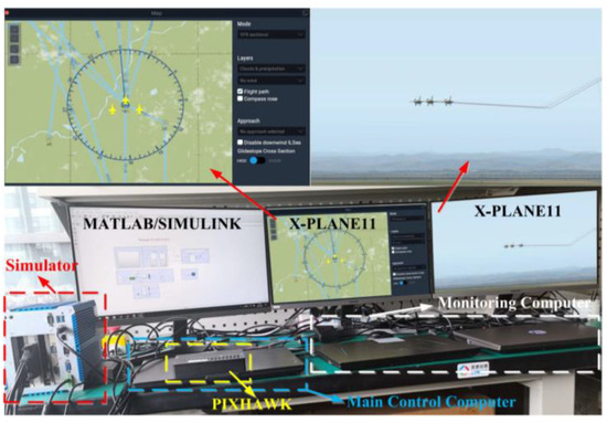
Figure 3. Experiment prototype of the Links-RT UAV platform.

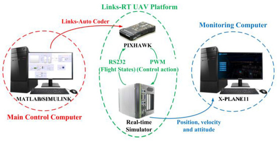
Figure 4. Relationship between functional units.

The desired path of the leader is defined by

$$\{\begin{array}{l}{x}_d=250\cos (0.02t)\\ y_d=250\sin (0.02t)\\ z_{\mathrm{d}}=0.5\mathrm{t}\end{array}$$

(153)

The initial position of the leader UAV is $p_0(0)=[-10.5,-0.9,-1]$, and the initial positions of the other two UAVs are $[1,-12.8,-1]$ and $[7,0.7,-0.8]$, respectively. The initial velocity of the follower UAVs is $V_{i0}=0\mathrm{m}/\mathrm{s}$, the initial values are taken as $r_{i0}=p_{i0}=q_{i0}=0\mathrm{rad}/\mathrm{s}$ and ${\varphi }_{i0}={\theta }_{i0}={\psi }_{i0}=0\mathrm{rad}$, respectively. The desired distance between the follower UAVs is chosen as $d_{12}=d_{23}=d_{31}=10\mathrm{m}$. The rigidity matrix of the formation is chosen as

$$R\left(p\right)=\left[\begin{array}{ccc}0& 1& 1\\ 1& 0& 1\\ 1& 1& 0\end{array}\right]$$

(154)

The external disturbance of the formation is $d_{i1}=0.1$, $d_{i2}=0.2$, $d_{i3}=0.15$, $d_{i4}=0.25$, and $d_{i5}=0.3$. The failure for the UAV#1 at t = 30 s is defined as

$$\{\begin{array}{l}{\rho }_{1f}=[1,1,1],\hfill \\ {\rho }_{1f}=[0.6,0.5,0.7],\hfill \end{array}\begin{array}{l}{u}_{1f}=0\mathrm{rad}\\ u_{1f}=0.13\mathrm{rad}\end{array}& \begin{array}{l}t<30\mathrm{s}\\ t\ge 30\mathrm{s}\end{array}$$

(155)

In the experiment, the maximum value of the actuator control input is $u_{i\max }=[100,1,1,1]$. The parameters of the controllers are shown in Table 1. The experimental simulation results are shown in Figure 5, Figure 6, Figure 7, Figure 8, Figure 9, Figure 10 and Figure 11.

Table 1. Parameters of controllers.

Parameter	Value	Parameter	Value
$k_1$	1.2	$c_{i1}$	0.8
$k_2$	0.6	$c_{i2}$	1
$K$	[1.5,0,0;0,2,0;0,0,2]	$c_{i3}$	0.8
${\tau }_{i1}$	0.01	${\eta }_{i1}$	1.2
${\tau }_{i2}$	0.01	${\eta }_{i2}$	1.2
${\tau }_{i3}$	0.01	${\eta }_{i3}$	1.3
${\tau }_{i4}$	0.02	${\mathrm{\Gamma }}_{i1}$	0.8
${\tau }_{i5}$	0.01	${\mathrm{\Gamma }}_{i2}$	0.5
${\tau }_{i6}$	0.01	${\mathrm{\Gamma }}_{i3}$	5
$k_{i1}$	1.2	${\mathrm{\Gamma }}_{i4}$	3
$k_{i2}$	3	${\mathrm{\Gamma }}_{i5}$	3
$k_{i3}$	1.8	${\mathrm{\Gamma }}_{i6}$	2
$k_{i4}$	2	$k_{Wi1}$	0.05
$k_{i5}$	1	$k_{Wi2}$	0.05
$k_{i6}$	1	$k_{Wi3}$	0.02
$k_{i7}$	1.5	$k_{Wi4}$	0.05
$k_{i8}$	2	$k_{Wi5}$	0.05
$k_{i9}$	2.5	$k_{Wi6}$	0.05
$k_{i10}$	2	$k_{wi1}$	100
$k_{i11}$	1.2	$k_{wi2}$	150
$k_{i12}$	0.9	$k_{wi3}$	150
$k_{i13}$	2.5	$k_{wi4}$	150
$k_{i14}$	4.5

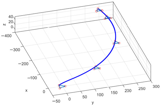
Figure 5. UAV formation path-tracking effect under input constraints. The red squares indicate UAV#i. The blue triangles indicate the formation configuration.

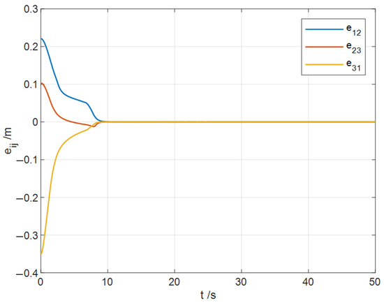
Figure 6. Formation distance error variation under input constraint.

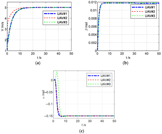
Figure 7. Formation UAV flight status under input constraints. (a) V_i response. (b) β_i response. (c) α_i response.

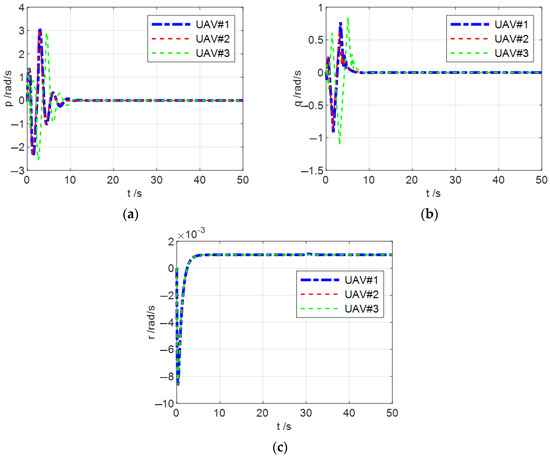
Figure 8. Angular velocity of formation UAV under input constraints. (a) p_i response. (b) q_i response. (c) r_i response.

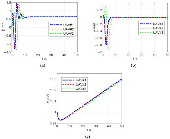
Figure 9. Formation UAV attitude angle under input constraints. (a) ${\varphi }_i$ response. (b) θ_i response. (c) ${\psi }_i$ response.

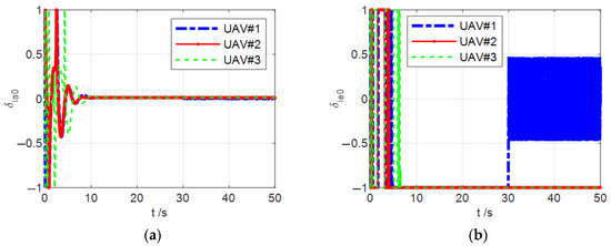
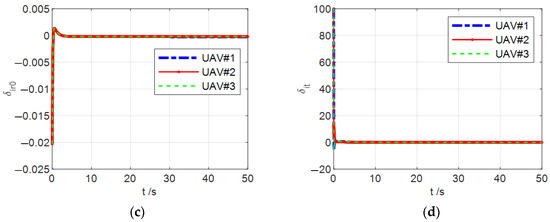
Figure 10. Formation UAV input control volume under input constraints. (a) ${\delta }_{ia0}$ response. (b) ${\delta }_{ie0}$ response. (c) ${\delta }_{ir0}$ response. (d) ${\delta }_{it}$ response.

Figure 11. Approximation error of RBFNN for uncertain terms under input constraint.

Remark 2.

When selecting the control parameters, it is first classified to determine which type the parameters belong to, and then they are selected according to the characteristics of each type of parameter and design experience. Through multiple simulation verifications, the optimal parameter value is finally determined according to the effect of the control response.

Figure 5 gives the UAV formation path tracking effect under input constraints. The blue line is the flight path of the leader which tracks the desired path defined by $x_d=250\cos (0.02t)$, $y_d=250\sin (0.02t)$, and $z_{\mathrm{d}}=0.5\mathrm{t}$. Figure 5 shows the tracking control effect considering the external disturbances and actuator failure under the input-constrained condition. It is observed that the tracking trajectory is relatively smooth considering the input constraint. The distance error of the formation is shown in Figure 6. It can be observed that the distance error of each UAV can converge to a finite value with the desired convergence rate at t = 10 s. It can be seen that the convergence rate is flat due to the consideration of the input constraint condition. In other words, within a short time after takeoff, the distance between the three UAVs reaches the desired formation distance $d_{12}=d_{23}=d_{31}=10\mathrm{m}$ and finally achieves the desired stable configuration. During this period, despite the influence of external interferences and input saturation, and the specific actuator failure of No. 1 UAV at t = 30 s, due to the role of the proposed distributed adaptive path-following controller, all these do not affect the effective formation of stable formations.

Figure 7, Figure 8 and Figure 9 show the flight states $V_i,{\alpha }_i,{\beta }_i,p_i,q_i,r_i,{\varphi }_i,{\theta }_i,{\psi }_i$ of UAV#1-UAV#3, and the values of each state of the UAV tend to stabilize after the initial formation generation process of the flight. From Figure 7c, it can be seen that the angle of attack on UAV#3 oscillated considerably at t = 3 s but returned to a stable state after 2 s. The relationship between the three angles is θ = γ + α. According to Equation (7b,c), it can be concluded that this is the result of an external disturbance $d_{i2}=0.2$. From Figure 8a,b and Figure 9a,b, it can be seen that the roll rate and pitch rate and the roll angle and pitch angle change dramatically within 5 s and become stable after 5 s. According to Equations (7c,d) and (9b,c), this is caused by unmodeled dynamics $f_{ip},f_{iq},f_{i\varphi }$ and external disturbances $d_{i4}=0.25,d_{i3}=0.15$. When the three UAVs are subjected to these effects, the ailerons and elevators need to produce certain roll moments and pitch moments to counteract their effects, respectively. After the action of the roll moment and pitch moments, the roll rate and pitch rate change, and then the roll angle and pitch angle change correspondingly, respectively. This is also reflected in Figure 10a,b. It can be seen that there is chattering in the responses of the roll rate and pitch rate and the roll angle and pitch angle due to the sliding mode controller. In addition, it can be seen that the actuator of UAV#1 is faulty at t = 30 s, and the control input is adjusted by the adaptive sliding mode controller. Despite these uncertain effects, in terms of the control performance, the states of the UAVs can change smoothly under the distributed adaptive path-following controller.

It can be observed from Figure 10 that the control inputs of each UAV can be kept within the maximum control input after considering the input constraint. At t = 30 s, there is a significant change in the control input of UAV#1 when it fails, and the control inputs of the other UAVs are minimally affected. Since this paper implements the fault-tolerant control of UAV actuator failures through an adaptive sliding mode controller, the control input has a chattering phenomenon. And in Figure 10, it can be seen that there is chattering in the control input due to the sliding mode controller, which is most obvious especially when the actuator fails, as a result of the introduction of the adaptive sliding-mode fault-tolerant controller, which needs to be studied in depth subsequently.

Figure 11 shows the approximation error of the RBFNN for the uncertainty terms, and it is observed that the approximation errors of the UAVs are bounded. At t = 30 s, the error of UAV#1 becomes significantly small under the RBFNN, which dealing with the uncertainties generated by the actuator failure. Generally, by introducing the adaptive sliding mode fault-tolerant controller, the approximation error of the RBFNN is obviously improved after the fault occurs. It can be seen that the proposed neural network controller can effectively approximate and compensate the model uncertainty terms $f_{iv}$, $f_{i\gamma }$, $f_{iq}$, $f_{ip}$, $f_{i\beta }$, and $f_{ir}$ and the external disturbances $d_{i1}=0.1$, $d_{i2}=0.2$, $d_{i3}=0.15$, and $d_{i4}=0.25$.

Remark 3.

Compared to the numerous existing formation control methods for the outer-loop position model expressed by the double-integrator form, this paper focuses on developing the distributed fault-tolerant formation flight control scheme for multiple 6-DOF fixed-wing UAVs against unknown aerodynamic parameters, actuator faults, and input saturations. To solve this controller design challenge, the distributed adaptive path-following controller for distance-based formation is first proposed. The path-following control strategy which combined the adaptive dynamic surface and neural network control technology was employed to approximate the uncertain disturbances of the environment and unmodeled dynamics. The auxiliary controller solved the stability of the formation control system under input limitations. In addition, by designing an adaptive sliding mode fault-tolerant controller, the stability of the formation flight was ensured in the case of actuator failures of the UAVs. The experimental simulation results have demonstrated the feasibility of the proposed controller for a multi-UAV system.

5. Conclusions and Future Works

In this paper, the distributed adaptive path-following control for distance-based formation was proposed for multiple fixed-wing UAVs under input saturations and actuator faults in a three-dimensional environment. By dividing the fixed-wing UAV model into the longitudinal dynamics containing the forward and vertical subsystems and the lateral–directional dynamics containing the lateral and sideslip angle subsystems, two adaptive fault-tolerant controllers are proposed to regulate the longitudinal and lateral–directional motions of multiple fixed-wing UAVs based on the distance-based formation control structure and dynamic surface control. The path-following control strategy which combined the adaptive dynamic surface and neural network control technology was proposed, where the uncertain disturbances of the environment and unmodeled dynamics can be approximated. The auxiliary controller solved the stability of the formation control system under input limitations. In addition, by designing an adaptive sliding mode fault-tolerant controller, the stability of the formation flight was ensured in the case of actuator failures of the UAVs. It was shown by the Lyapunov method that all signals are ultimately semi-globally and uniformly bounded and the tracking performance can be achieved even when the fixed-wing UAVs are subjected to the input saturations and actuator faults. Finally, the experimental simulation validation was provided to demonstrate the feasibility and superiority of the proposed control scheme.

In the early stage of formation and after the actuator failure of a UAV, the UAV will often have a large flight action, which may lead to the collision of the UAV in the formation. Designing a collision avoidance controller is the key technology to realize large-scale formation flights, which is one of the next research directions. In addition, the experimental simulation of this paper only considers the formation flight of three UAVs, and more UAV formation flight simulations is also a direction of future work. Furthermore, the proposed controller has many control parameters, so how to simplify the control parameters is one of the key problems to be solved in the future.

References

- Ouyang, Q.; Wu, Z.; Cong, Y.; Wang, Z. Formation control of unmanned aerial vehicle swarms: A comprehensive review. Asian J. Control 2023, 25, 570–593. [Google Scholar] [CrossRef]
- Chen, L.; Xiao, J.; Lin, R.C.H.; Feroskhan, M. Angle-Constrained Formation Maneuvering of Unmanned Aerial Vehicles. IEEE Trans. Control Syst. Technol. 2023, 31, 1733–1746. [Google Scholar] [CrossRef]
- Shao, X.L.; Liu, H.C.; Zhang, W.D.; Zhao, J.; Zhang, Q.Z. Path driven formation-containment control of multiple UAVs: A path-following framework. Aerosp. Sci. Technol. 2023, 135, 108168. [Google Scholar] [CrossRef]
- Nian, X.H.; Zhou, W.X.; Li, S.L.; Wu, H.Y. 2-D path following for fixed wing UAV using global fast terminal sliding mode control. ISA Trans. 2023, 136, 162–172. [Google Scholar] [CrossRef] [PubMed]
- Chung, S.-J.; Paranjape, A.A.; Dames, P.; Shen, S.; Kumar, V. A Survey on Aerial Swarm Robotics. IEEE Trans. Robot. 2018, 34, 837–855. [Google Scholar] [CrossRef]
- Cabecinhas, D.; Cunha, R.; Silvestre, C. Rotorcraft path following control for extended flight envelope coverage. In Proceedings of the 48th IEEE Conference on Decision and Control, CDC 2009, Combined with the 28th Chinese Control Conference, Shanghai, China, 15–18 December 2009; pp. 16–18. [Google Scholar]
- Cabecinhas, D.; Cunha, R.; Silvestre, C. A Globally Stabilizing Path Following Controller for Rotorcraft with Wind Disturbance Rejection. IEEE Trans. Control Syst. Technol. 2015, 23, 708–714. [Google Scholar] [CrossRef]
- Klausen, K.; Fossen, T.I.; Johansen, T.A.; Aguiar, A.P. Cooperative path-following for multirotor UAVs with a suspended payload. In Proceedings of the IEEE Conference on Control Applications (CCA), Sydney, Australia, 21–23 September 2015; pp. 1354–1360. [Google Scholar]
- Akkinapalli, V.S.; Niermeyer, P.; Lohmann, B.; Holzapfel, F. Adaptive nonlinear design plant uncertainty cancellation for a multirotor. In Proceedings of the International Conference on Unmanned Aircraft Systems (ICUAS), Arlington, VA, USA, 7–10 June 2016; pp. 1102–1110. [Google Scholar]
- Rucco, A.; Aguiar, A.P.; Hauser, J. Trajectory optimization for constrained UAVs: A Virtual Target Vehicle approach. In Proceedings of the International Conference on Unmanned Aircraft Systems (ICUAS), Denver, CO, USA, 9–12 June 2015; pp. 236–245. [Google Scholar]
- Rucco, A.; Aguiar, A.P.; Pereira, F.L.; de Sousa, J.B. A Predictive Path-Following Approach for Fixed-Wing Unmanned Aerial Vehicles in Presence of Wind Disturbances. In Proceedings of the Second Iberian Robotics Conference, Lisbon, Portugal, 19–21 November 2015. [Google Scholar]
- Desai, J.P.; Ostrowski, J.P.; Kumar, V. Controlling formations of multiple mobile robots. In Proceedings of the IEEE International Conference on Robotics and Automation (Cat. No.98CH36146), Leuven, Belgium, 20–20 May 1998; pp. 2864–2869. [Google Scholar]
- Byrnes, C.I.; Isidori, A. Asymptotic stabilization of minimum phase nonlinear systems. IEEE Trans. Autom. Control 1991, 36, 1122–1137. [Google Scholar] [CrossRef]
- Edwards, C.; Spurgeon, S. Sliding Mode Control: Theory And Applications; CRC Press: Boca Raton, FL, USA, 1998. [Google Scholar]
- Shah, M.Z.; Samar, R.; Bhatti, A.I. Lateral track control of UAVs using the sliding mode approach: From design to flight testing. Trans. Inst. Meas. Control 2014, 37, 457–474. [Google Scholar] [CrossRef]
- Thanh, H.L.N.N.; Vu, M.T.; Mung, N.X.; Nguyen, N.P.; Phuong, N.T. Perturbation observer-based robust control using a multiple sliding surfaces for nonlinear systems with influences of matched and unmatched uncertainties. Mathematics 2020, 8, 1371. [Google Scholar] [CrossRef]
- Alattas, K.A.; Mobayen, S.; Din, S.U.; Asad, J.H.; Fekih, A.; Assawinchaichote, W.; Vu, M.T. Design of a non-singular adaptive integral-type finite time tracking control for nonlinear systems with external disturbances. IEEE Access 2021, 9, 102091–102103. [Google Scholar] [CrossRef]
- Mofid, O.; Amirkhani, S.; Din, S.U.; Mobayen, S.; Vu, M.T.; Assawinchaichote, W. Finite-time convergence of perturbed nonlinear systems using adaptive barrier-function nonsingular sliding mode control with experimental validation. J. Vib. Control 2023, 29, 3326–3339. [Google Scholar] [CrossRef]
- Rojsiraphisal, T.; Mobayen, S.; Asad, J.H.; Vu, M.T.; Chang, A.; Puangmalai, J. Fast terminal sliding control of underactuated robotic systems based on disturbance observer with experimental validation. Mathematics 2021, 9, 1935. [Google Scholar] [CrossRef]
- Alattas, K.A.; Vu, M.T.; Mofid, O.; El-Sousy, F.F.M.; Alanazi, A.K.; Awrejcewicz, J.; Mobayen, S. Adaptive nonsingular terminal sliding mode control for performance improvement of perturbed nonlinear systems. Mathematics 2022, 10, 1064. [Google Scholar] [CrossRef]
- Mobayen, S.; Bayat, F.; Din, S.U.; Vu, M.T. Barrier function-based adaptive nonsingular terminal sliding mode control technique for a class of disturbed nonlinear systems. ISA Trans. 2023, 134, 481–496. [Google Scholar] [CrossRef]
- Ghaffari, V.; Mobayen, S.; Din, S.U.; Rojsiraphisal, T.; Vu, M.T. Robust tracking composite nonlinear feedback controller design for time-delay uncertain systems in the presence of input saturation. ISA Trans. 2022, 129, 88–99. [Google Scholar] [CrossRef]
- Roza, A.; Maggiore, M. Path following controller for a quadrotor helicopter. In Proceedings of the American Control Conference (ACC), Montreal, QC, Canada, 27–29 June 2012; pp. 4655–4660. [Google Scholar]
- Raffo, G.V.; Ortega, M.G.; Rubio, F.R. Backstepping/nonlinear H∞ control for path tracking of a quadrotor unmanned aerial vehicle. In Proceedings of the American Control Conference, Seattle, WA, USA, 11–13 June 2008; pp. 3356–3361. [Google Scholar]
- Kaminer, I.; Yakimenko, O.; Pascoal, A.; Ghabcheloo, R. Path Generation, Path Following and Coordinated Control for TimeCritical Missions of Multiple UAVs. In Proceedings of the 2006 American Control Conference, Minneapolis, MN, USA, 14–16 June 2006; pp. 4906–4913. [Google Scholar]
- Xargay, E.; Kaminer, I.; Pascoal, A.; Hovakimyan, N.; Dobrokhodov, V.; Cichella, V.; Aguiar, A.P.; Ghabcheloo, R. Time-Critical Cooperative Path Following of Multiple Unmanned Aerial Vehicles over Time-Varying Networks. J. Guid. Control Dyn. 2013, 36, 499–516. [Google Scholar] [CrossRef]
- Chen, H.; Cong, Y.; Wang, X.; Xu, X.; Shen, L. Coordinated Path Following Control of Fixed-wing Unmanned Aerial Vehicles. IEEE Trans. Cybern. 2019, 52, 2540–2554. [Google Scholar]
- Ren, W.; Atkins, E. Distributed multi-vehicle coordinated control via local information exchange. Int. J. Robust Nonlinear Control 2007, 17, 1002–1033. [Google Scholar] [CrossRef]
- Meng, Z.; Anderson, B.D.; Hirche, S. Formation control with mismatched compasses. Automatica 2016, 69, 232–241. [Google Scholar] [CrossRef]
- Ramazani, S.; Selmic, R.; de Queiroz, M. Rigidity-based multiagent layered formation control. IEEE Trans. Cybern. 2017, 47, 1902–1913. [Google Scholar] [CrossRef]
- Cai, X.; de Queiroz, M. Rigidity-based stabilization of multi-agent formations. J. Dyn. Syst. Meas. Control 2014, 136, 014502. [Google Scholar] [CrossRef]
- Dorfler, F.; Francis, B. Geometric analysis of the formation problem for autonomous robots. IEEE Trans. Autom. Control 2010, 5, 2379–2384. [Google Scholar] [CrossRef]
- Krick, L.; Broucke, M.E.; Francis, B.A. Stabilisation of infinitesimally rigid formations of multi-robot networks. Int. J. Control 2009, 82, 423–439. [Google Scholar] [CrossRef]
- Oh, K.K.; Ahn, H.-S. Formation control of mobile agents based on inter-agent distance dynamics. Automatica 2011, 47, 2306–2312. [Google Scholar] [CrossRef]
- Babazadeh, R.; Selmic, R. Distance-based multi-agent formation control with energy constraints using SDRE. IEEE Trans. Aerosp. Electron. Syst. 2019, 56, 41–56. [Google Scholar] [CrossRef]
- Cai, X.; Queiroz, M. Formation maneuvering and target interception for multi-agent systems via rigid graphs. Asian J. Control 2015, 17, 1174–1186. [Google Scholar] [CrossRef]
- Aryankia, K.; Selmic, R.R. Neuro-Adaptive Formation Control and Target Tracking for Nonlinear Multi-Agent Systems with Time-Delay. IEEE Control Syst. Lett. 2021, 5, 791–796. [Google Scholar] [CrossRef]
- Vu, D.V.; Trinh, M.H.; Ahn, H.S. Distance--Based Formation Tracking with Unknown Bounded Reference Velocities. In Proceedings of the 20th International Conference on Control, Automation and Systems (ICCAS), Busan, Republic of Korea, 13–16 October 2020; pp. 524–529. [Google Scholar]
- Yu, Z.; Qu, Y.; Zhang, Y. Distributed Fault-Tolerant Cooperative Control for Multi-UAVs Under Actuator Fault and Input Saturation. IEEE Trans. Control Syst. Technol. 2018, 27, 2417–2429. [Google Scholar] [CrossRef]
- Chang, S.J.; Lee, J.Y.; Park, J.B.; Choi, Y.H. An online fault tolerant actor-critic neuro-control for a class of nonlinear systems using neural network HJB approach. Int. J. Control Autom. Syst. 2015, 13, 311–318. [Google Scholar] [CrossRef]
- Yu, Z.; Liu, Z.; Zhang, Y.; Qu, Y.; Su, C.Y. Distributed Finite-Time Fault-Tolerant Containment Control for Multiple Unmanned Aerial Vehicles. IEEE Trans. Neural Netw. Learn. Syst. 2019, 99, 2077–2091. [Google Scholar] [CrossRef]
- Hou, Z.; Fantoni, I. Leader-follower formation saturatedcontrol for multiple quadrotors with switching topology. In Proceedings of the Workshop on Research, Education and Development of Unmanned Aerial Systems (RED-UAS), Cancun, Mexico, 23–25 November 2015; pp. 8–14. [Google Scholar]
- Xiang, X.; Liu, C.; Su, H.; Zhang, Q. On decentralized adaptive full-order slidingmode control of multiple UAVs. ISA Trans. 2017, 71, 196–205. [Google Scholar] [CrossRef] [PubMed]
- Asimow, L.; Roth, B. The rigidity of graphs, II. J. Math. Anal. Appl. 1979, 68, 171–190. [Google Scholar] [CrossRef]
- Dogan, A.; Venkataramanan, S. Nonlinear Control for Reconfiguration of Unmanned-Aerial-Vehicle Formation. J. Guid. Control Dyn. 2005, 28, 667–678. [Google Scholar] [CrossRef][Green Version]
- Yu, Z.; Zhang, Y.; Jiang, B.; Yu, X.; Fu, J.; Jin, Y.; Chai, T. Distributed adaptive fault-tolerant close formation flight control of multiple trailing fixed-wing UAVs. ISA Trans. 2020, 106, 181–199. [Google Scholar] [CrossRef] [PubMed]
- Yu, Z.; Qu, Y.; Zhang, Y. Safe Control of Trailing UAV in Close Formation Flight against Actuator Fault and Wake Vortex Effect. Aerosp. EnceTechnol. 2018, 77, 189–205. [Google Scholar] [CrossRef]
- Payne, A.N. Adaptive one-step-ahead control subject to an input-amplitude constraint. Int. J. Control 1986, 43, 1257–1269. [Google Scholar] [CrossRef]
Disclaimer/Publisher’s Note: The statements, opinions and data contained in all publications are solely those of the individual author(s) and contributor(s) and not of MDPI and/or the editor(s). MDPI and/or the editor(s) disclaim responsibility for any injury to people or property resulting from any ideas, methods, instructions or products referred to in the content. |
© 2023 by the authors. Licensee MDPI, Basel, Switzerland. This article is an open access article distributed under the terms and conditions of the Creative Commons Attribution (CC BY) license (https://creativecommons.org/licenses/by/4.0/).