A Full Envelope Robust Linear Parameter-Varying Control Method for Aircraft Engines

Abstract

In order to solve the problem of full flight envelope control for aircraft engines, the design of a linear parameter-varying (LPV) controller is described in this paper. First, according to the nonlinear aerodynamic model of the aircraft engine, the LPV engine model for the controller design is obtained through the Jacobian linearization and fitting technique. Then, the flight envelope is divided into several sub-regions, and the intersection of adjacent sub-regions is not empty. The sub-region LPV controller is designed using the parameter-dependent Lyapunov function (PDLF)-based LPV synthesis method, while eliminating the dependence of the LPV controller on scheduling parameter derivatives. In order to ensure the stability and performance of the aircraft engine across the full flight envelope, a mixing LPV control method is proposed to design the LPV controller in the overall region. The effectiveness of the proposed method is verified by simulating a dual-spool turbofan engine on a nonlinear component level model and comparing the proposed method with the gain scheduling based on PI and H_∞ point design.

1. Introduction

A safe, reliable, and efficient aircraft engine control system is crucial for modern aircraft to complete high-performance maneuvers under various atmospheric environmental conditions and flight mission requirements. The full authority digital engine control (FADEC) systems [1] can better utilize the potential of the engine at a small cost without adding additional hardware.

The dynamic behavior of aircraft engines varies greatly with changes in working environment conditions, such as the flight speed, inlet temperature, pressure, pilot throttle lever commands, etc. Therefore, it is obvious that the performance requirements for aircraft engines cannot be met using a fixed gain engine controller throughout the entire flight envelope range. The control algorithm widely used in the aviation industry today is the traditional gain scheduling control scheme, which utilizes the Jacobian linearization engine model. And the controller gain is scheduled online from a series of LTI controllers designed based on local linearization models at the design-point, according to changes in operating conditions. A sliding mode control (SMC) method is used for the set-point tracking of aircraft engines in references [2,3]. But it is only designed for a fixed operating point condition and is not suitable for situations where the engine operating point changes.

In fact, the traditional gain scheduling control technique can connect LTI controllers at various design-points through appropriate scheduling algorithms, such as linear interpolation. However, the stability and performance at off-design points cannot be guaranteed using this method. Generally, a large number of repetitive designs are required by the traditional gain scheduling technique, which is very cumbersome. In addition, the stability and performance of the closed-loop systems at different design points require extensive simulation to verify [4,5]. To address the shortcomings of traditional gain scheduling design, the concept of a linear parameter-varying (LPV) system is proposed in reference [5]. The LPV system is composed of a family of linear systems, whose dynamic characteristics are fixed, known functions of measurable scheduling variables. A review of the research on LPV control theory can be found in the literature [6,7]. At present, LPV control technology mainly includes linear-fractional transformation (LFT)-based and Lyapunov-based LPV techniques. The former [8,9,10] solves LPV controllers based on the small gain conditions. In this paper, the LPV control technique based on Lyapunov theory is adopted because it has less conservatism than the former. The gain scheduling controller design is used in the literature [11,12] to ensure quadratic H_∞ performance for LPV systems. But this method has been proven to be conservative [13], as it uses a single quadratic Lyapunov function (SQLF) throughout the entire range of scheduling parameters, which allows for an infinite rate of variation in the scheduling parameters. To reduce conservatism, the literature [13,14,15,16] proposes an LPV synthesis strategy using the parameter-dependent Lyapunov function (PDLF), which has been proven to be effective by utilizing the rate of change information of scheduling variables. Unfortunately, the introduction of PDLF in LPV synthesis also brought two troubles. First, the LPV controller calculated by the PDLF method contains the derivative information of scheduling variables, which is not conducive to the implementation of LPV control because of the unknown derivative of scheduling variables in reality. An approach to eliminating the derivative information in the LPV controllers has been used in the literature [17] by imposing constraints on two symmetric matrix variables X(θ) and Y(θ), that is, one of them is required to be parameter-independent. The second hassle is that the LPV control by the PDLF method often requires a greater computational burden because of the difficulty of solving infinite-dimensional linear matrix inequalities (LMIs) optimization problems, especially for LPV systems with multiple scheduling parameters.

At present, there is a large amount of literature on the research of the robust LPV control technique in various fields, such as missile autopilots [18,19], aircraft [20], automobiles [21], robotic manipulators [22], etc. However, there is relatively little research on the LPV control of aircraft engines. The robust H_∞ gain scheduling control method has been adopted in the literature [23] to develop the controller for aircraft engines. However, this is only the traditional gain scheduling technique, which has the drawbacks described above. The literature [24] designs LPV controllers for a turbofan engine based on SQLF and PDLF methods, respectively. And the fact that the SQLF method is more conservative than the PDLF method has been verified through nonlinear simulation analysis in the literature [24]. However, the LPV controllers are only designed at sea level, zero flight Mach number conditions, that is, only changes in engine power are considered, without considering changes in flight conditions. Moreover, it did not specify the controller design method under other flight conditions.

Due to the aircraft engine operating within a wide flight envelope, its dynamic characteristics typically require three scheduling parameters: the engine power, altitude, and flight Mach number [25]. Although the PDLF-based LPV control technique has less conservatism for aircraft engine control, its solution is difficult because of the presence of multiple scheduling parameters. This paper proposes a mixing LPV control method that divides scheduling variables into two groups and partitions the operating envelope, requiring the intersection of an adjacent sub-region to be non-empty. Due to the fact that the LPV controller in the sub-region only relies on common scheduling parameters, this method is beneficial in reducing the burden of solving LMIs based on the PDLF method. In addition, the stability and performance of the closed-loop systems under different flight conditions for the engine can be guaranteed using this method.

The outline of the paper is as follows. The preliminaries of LPV control are given in Section 2. The methods for establishing the turbofan engine LPV model for controller design are provided in Section 3. Section 4 presents the design of a sub-region LPV controller based on the PDLF method. Section 5 provides the design of the overall region LPV controller using the mixing LPV control technique. In Section 6, the simulation analyses of the component level model of the aircraft engine are described, using the proposed method, proportional plus integral (PI) design, and robust H_∞ point design methods, respectively. Finally, Section 7 gives the conclusion of the paper.

2. Preliminaries

The following notations will be used in this paper. ${ℝ}_{+}$ denotes the set of positive real numbers. ${ℝ}^s$ denotes the set of s-dimensional real numbers. ${\mathbb{S}}^n$ indicates the set of real, symmetric matrices with dimension $n\times n$. ${\mathbb{S}}_{+}^n$ denotes the set of real, symmetric positive definite matrices with dimension $n\times n$. Given two sets $M$ and $N$, $M-N$ represents a set where elements belong to $M$ but not to $N$, and $M\times N$ denotes the Cartesian product of sets. Given two matrices $X_1$ and $X_2$, $diag\left\{X_1,X_2\right\}$ is the block-diagonal matrix. In the symmetric matrix, $\star$ represents the off-diagonal term, which can be known from symmetry.

In this section, we begin with a brief statement of the LPV control in the framework of robust control. Given an LPV system with general parameter dependency,

$$\begin{array}{l}\dot{x}=A\left(\theta \right)x+B_1\left(\theta \right)w+B_2\left(\theta \right)u\\ z=C_1\left(\theta \right)x+D_{11}\left(\theta \right)w+D_{12}\left(\theta \right)u\\ y=C_2\left(\theta \right)x+D_{21}\left(\theta \right)w+D_{22}\left(\theta \right)u\end{array}$$

(1)

The time-varying parameter vector $\theta \left(t\right)\in {ℝ}^s$ in Equation (1) is called the scheduling parameter, which cannot be known in advance. It is assumed that $\theta \left(t\right)$ is measurable in this paper. $x\left(t\right)\in {ℝ}^n$, $y\left(t\right)\in {ℝ}^{n_y}$, and $u\left(t\right)\in {ℝ}^{n_u}$ represent the plant state, output, and input variable, respectively. $z\left(t\right)\in {ℝ}^{n_z}$ and $w\left(t\right)\in {ℝ}^{n_w}$ represent the performance output and input variable, respectively. The coefficient matrices $A\left(\theta \right)$, $B_1\left(\theta \right)$, $\dots$, $D_{22}\left(\theta \right)$ in Equation (1), which have appropriate dimensions, are fixed functions with respect to $\theta \left(t\right)$. It is assumed that $\theta \left(t\right)$ and its derivative $\dot{\theta }\left(t\right)$ lie in the following hyper-rectangular sets

$$\theta \left(t\right)\in \mathrm{\Theta },\mathrm{\Theta }:=\left\{\theta \in {ℝ}^s:{\theta }_i\in \left[{\underset{\_}{\theta }}_i, {\overline{\theta }}_i\right],i\in 1,\cdots ,s\right\}$$

(2)

$$\dot{\theta }\left(t\right)\in {\mathrm{\Theta }}_d,{\mathrm{\Theta }}_d:=\left\{\dot{\theta }\in {ℝ}^s:{\dot{\theta }}_i\in \left[{\underset{\_}{v}}_i, {\overline{v}}_i\right],i\in 1,\cdots ,s\right\}$$

(3)

Hereafter, the dependence of the time-varying parameters $\theta$ and $\dot{\theta }$ on time will be omitted for simplicity.

The following two assumptions are made for synthesizing the LPV controllers:

(a)

The pairs $\left(A\left(\theta \right),B_2\left(\theta \right)\right)$ and $\left(A\left(\theta \right),C_2\left(\theta \right)\right)$ are stabilizable and detectable for any $\theta \in \mathrm{\Theta }$, respectively.

(b)

$D_{22}\left(\theta \right)=0$ for any $\theta \in \mathrm{\Theta }$.

In order to ensure that the LPV system (1) can be stabilized by an LPV controller (4), it is necessary for system (1) to satisfy the assumption (a). The assumption (b) is only for the convenience of deriving formulas when synthesizing the LPV controllers.

The existence of an LPV controller in the following form is assumed:

$$\begin{array}{c}{\dot{x}}_K=A_K\left(\theta ,\dot{\theta }\right)x_K+B_K\left(\theta ,\dot{\theta }\right)y\\ u=C_K\left(\theta ,\dot{\theta }\right)x_K+D_K\left(\theta ,\dot{\theta }\right)y\end{array}$$

(4)

where the coefficient matrices $A_K\left(\theta ,\dot{\theta }\right)$, $B_K\left(\theta ,\dot{\theta }\right)$, $C_K\left(\theta ,\dot{\theta }\right)$, and $D_K\left(\theta ,\dot{\theta }\right)$ are bounded, continuous functions of $\theta$ and its derivative $\dot{\theta }$. $x_K\in {ℝ}^k$ is the LPV controller state vector. In this paper, only the case of full order dynamic output feedback LPV control is considered, so $k=n$.

Then, the closed-loop LPV system from $w$ to $z$ can be obtained

$$\begin{array}{c}{\dot{x}}_{cl}=A_{cl}\left(\theta \right)x_{cl}+B_{cl}\left(\theta \right)w\\ z=C_{cl}\left(\theta \right)x_{cl}+D_{cl}\left(\theta \right)w\end{array}$$

(5)

where the state vector of the above LPV system is denoted by $x_{cl}^T=\left[x^T,x_K^T\right]$. Substituting (1) and (4) into (5), the coefficient matrices of Equation (5) can be given below.

$$\{\begin{array}{l}{A}_{cl}\left(\theta \right)=\left[\begin{array}{cc}A\left(\theta \right)+B_2\left(\theta \right)D_K\left(\theta \right)C_2\left(\theta \right)& B_2\left(\theta \right)C_K\left(\theta \right)\\ B_K\left(\theta \right)C_2\left(\theta \right)& A_K\left(\theta \right)\end{array}\right]\hfill \\ B_{cl}\left(\theta \right)=\left[\begin{array}{c}{B}_1\left(\theta \right)+B_2\left(\theta \right)D_K\left(\theta \right)D_{21}\left(\theta \right)\\ B_K\left(\theta \right)D_{21}\left(\theta \right)\end{array}\right]\hfill \\ C_{cl}\left(\theta \right)=\left[\begin{array}{cc}{C}_1\left(\theta \right)+D_{12}\left(\theta \right)D_K\left(\theta \right)C_2\left(\theta \right)& D_{12}\left(\theta \right)C_K\left(\theta \right)\end{array}\right]\hfill \\ D_{cl}\left(\theta \right)=D_{11}\left(\theta \right)+D_{12}\left(\theta \right)D_K\left(\theta \right)D_{21}\left(\theta \right)\hfill \end{array}$$

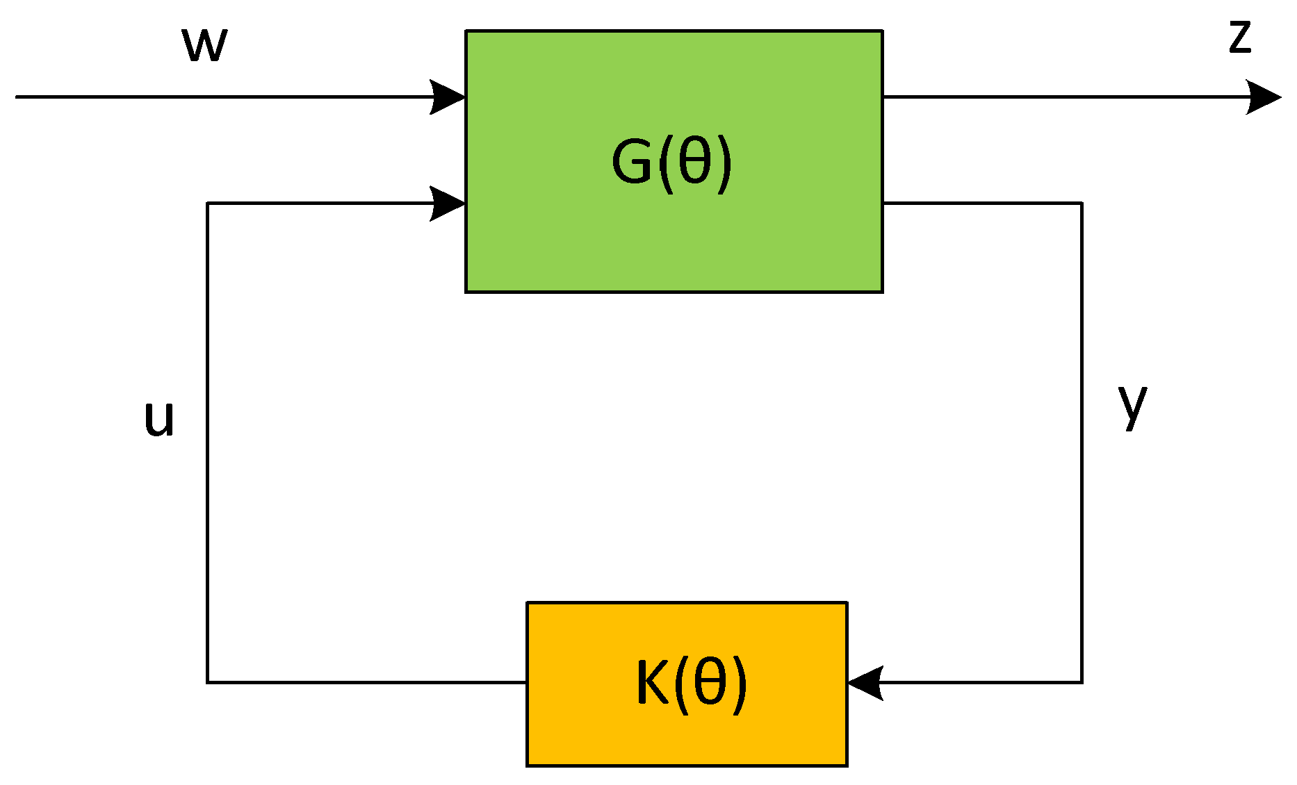
Figure 1 is a diagram of robust LPV control systems. The Induced ${ℒ}_2$ performance of the closed-loop LPV system (5) can be defined by (6).

$$\underset{\theta \in \mathrm{\Theta },w\in {ℒ}_2,{\Vert w\Vert }_2\ne 0}{sup}\frac{{\Vert z\Vert }_2}{{\Vert w\Vert }_2}\le \gamma$$

(6)

Then, the parameter-dependent quadratic LPV $\gamma$–performance problem [13] using PDLF is given by the following Lemma.

Lemma 1. 

For an LPV system (1) with scheduling variables satisfying (2) and (3), the parameter-dependent closed-loop LPV system (5) is stabilized by LPV controller (4) and acquires the induced ${ℒ}_2$ performance level $\gamma$ if there exists a matrix $P\left(\theta \right)\in {\mathbb{S}}_{+}^n$, such that the following LMI conditions are satisfied for any allowable parameter trajectories $\left(\theta ,\dot{\theta }\right)\in \mathrm{\Theta }\times {\mathrm{\Theta }}_d$.

$$P\left(\theta \right)>0,\forall \theta \in \mathrm{\Theta }$$

(7)

$${\mathbb{F}}_{BRL}\left(P\left(\theta \right),\gamma \right)<0$$

(8)

where

$${\mathbb{F}}_{BRL}\left(P\left(\theta \right),\gamma \right)=\left[\begin{array}{ccc}P\left(\theta \right)A_{cl}^T\left(\theta \right)+A_{cl}\left(\theta \right)P\left(\theta \right)-{\displaystyle \sum _{i=1}^s\left(\left\{{\underset{\_}{v}}_i, {\overline{v}}_i\right\}\frac{\partial P\left(\theta \right)}{\partial {\theta }_i}\right)}& B_{cl}\left(\theta \right)& P\left(\theta \right)C_{cl}^T\left(\theta \right)\\ B_{cl}^T\left(\theta \right)& -\gamma I_{n_w}& D_{cl}^T\left(\theta \right)\\ C_{cl}\left(\theta \right)P\left(\theta \right)& D_{cl}\left(\theta \right)& -\gamma I_{n_z}\end{array}\right]$$

(9)

Remark 1. 

Lemma 1 is the extended version of the famous Bounded Real Lemma (BRL). The notation ${\displaystyle \sum _{i=1}^s\left(\left\{{\underset{\_}{v}}_i, {\overline{v}}_i\right\}\frac{\partial P\left(\theta \right)}{\partial {\theta }_i}\right)}$ in LMI (9) means that every combination of ${\underset{\_}{v}}_i\frac{\partial P\left(\theta \right)}{\partial {\theta }_i}$ and ${\overline{v}}_i\frac{\partial P\left(\theta \right)}{\partial {\theta }_i}$ should be included.

3. LPV Modeling for Aircraft Engines

Before developing the LPV controller, it is necessary to first establish a model of the aircraft engine. Unlike other controlled plants, the dynamic behavior of aircraft engines cannot be represented accurately by an analytical expression. For research on aircraft engine control, the mainstream approach is to establish a nonlinear component level model (CLM) that accurately describes the steady-state and transient behavior of aircraft engines throughout a full operating envelope and then linearize the CLM to obtain the linearized engine model that is convenient for control law design.

As depicted in Figure 2, the commercial dual-shaft turbofan engine with a high bypass ratio, whose major components include the inlet, fan, low-pressure compressor (LPC), high-pressure compressor (HPC), combustor, high-pressure turbine (HPT), low-pressure turbine (LPT), and exhaust nozzle, is studied in this paper. By establishing the steady-state model of each engine component and utilizing the flow continuity, pressure, and energy balance conditions of each section of the engine, the final CLM can be obtained [26,27]. It is assumed that the CLM can be expressed as

$$\begin{array}{l}\dot{x}=f\left(x,u\right)\\ y=g\left(x,u\right)\end{array}$$

(10)

The engine dynamics are represented by the nonlinear functions $f(\cdot )$ and $g(\cdot )$. The linear engine model of the equilibrium point $\left(x_0, u_0,y_0\right)$ can be obtained as Equation (11) by the Jacobian linearization method.

$$\begin{array}{l}\mathrm{\Delta }\dot{x}=A\mathrm{\Delta }x+B\mathrm{\Delta }u\\ \mathrm{\Delta }y=C\mathrm{\Delta }x+D\mathrm{\Delta }u\end{array}$$

(11)

The symbol $\mathrm{\Delta }$ denotes the difference between the transient value and the design point value of the variable. For example, $\mathrm{\Delta }x=x-x_0$, and the definitions of $\mathrm{\Delta }u$ and $\mathrm{\Delta }y$ are similar. $x^T=\left[n_L,n_H\right]$, $u=W_f$, and $y^T=\left[n_L,n_H\right]$ represent the state variable, control variable, and output variable, respectively. $W_f$, $n_H$, and $n_L$ denote the fuel flow of the engine, high-pressure shaft speed, and low-pressure shaft speed, respectively. In reference [28], the coefficient matrices $\left(A,B,C,D\right)$ of state space Equation (11) at an operating point $\left(x_0, u_0,y_0\right)$ are calculated by the Jacobian linearization method. However, the results calculated by this method are not accurate, so the fitting method [26] is adopted in this paper. The fitting method assumes that the output responses of the small deviation linear model and CLM are equal if the same small step disturbance input signal $\mathrm{\Delta }u$ is applied to the system. Then, the coefficient matrices can be calculated by optimizing Equations (12)–(16) using the least squares method. $y_{lin}$ and $y_{non}$ represent the output response of the linear engine model and CLM to the same input at the same steady-state point, respectively. The solving process of Equations (12)–(16) can be performed using some nonlinear optimization algorithms, such as the fmincon function in the Matlab optimization toolbox.

$$min J={\displaystyle \sum {\left[\mathrm{\Delta }{y}_{non}-\mathrm{\Delta }{y}_{lin}\right]}^T\left[\mathrm{\Delta }{y}_{non}-\mathrm{\Delta }{y}_{lin}\right]}$$

(12)

$$\begin{array}{ll}\mathrm{\Delta }{y}_{lin}& =C\mathrm{\Delta }x+D\mathrm{\Delta }u\\ & =C\left[\begin{array}{l}\mathrm{\Delta }{n}_L\\ \mathrm{\Delta }{n}_H\end{array}\right]+D\mathrm{\Delta }{W}_f\end{array}$$

(13)

$$\mathrm{\Delta }{n}_L=\mathrm{\Delta }{W}_f\left[\frac{\left(s_1-a_{22}\right)b_1+a_{12}{b}_2}{s_1\left(s_1-s_2\right)}{e}^{s_{1}t}+\frac{\left(s_2-a_{22}\right)b_1+a_{12}{b}_2}{s_2\left(s_2-s_1\right)}{e}^{s_{2}t}+\frac{a_{12}{b}_2-a_{22}{b}_1}{s_1{s}_2}\right]$$

(14)

$$\mathrm{\Delta }{n}_H=\mathrm{\Delta }{W}_f\left[\frac{\left(s_1-a_{11}\right)b_2+a_{21}{b}_1}{s_1\left(s_1-s_2\right)}{e}^{s_{1}t}+\frac{\left(s_2-a_{11}\right)b_2+a_{21}{b}_1}{s_2\left(s_2-s_1\right)}{e}^{s_{2}t}+\frac{a_{21}{b}_1-a_{11}{b}_2}{s_1{s}_2}\right]$$

(15)

$$\{\begin{array}{l}{s}_1+s_2=a_{11}+a_{22}\\ s_1{s}_2=a_{11}{a}_{22}-a_{12}{a}_{21}\end{array}$$

(16)

$s_1$ and $s_2$ in Equations (14)–(16) are the eigenvalues of the matrix $A$. And $A=\left[\begin{array}{cc}{a}_{11}& a_{12}\\ a_{21}& a_{22}\end{array}\right]$, $B=\left[\begin{array}{c}{b}_1\\ b_2\end{array}\right]$.

The brief derivation process of Equations (14)–(16) is given below.

For the system $\mathrm{\Delta }\dot{x}=A\mathrm{\Delta }x+B\mathrm{\Delta }u$, $x\left(0\right)=0$, take the Laplace transform on both sides of the system to obtain

$$\begin{array}{c}\mathrm{\Delta }\mathcal{X}\left(s\right)={\left(sI-\mathbf{A}\right)}^{-1}B\mathrm{\Delta }\mathcal{U}\left(s\right)\\ ={\left[\begin{array}{cc}s-a_{11}& -a_{12}\\ -a_{21}& s-a_{22}\end{array}\right]}^{-1}\left[\begin{array}{c}{b}_1\\ b_2\end{array}\right]\mathrm{\Delta }\mathcal{U}\left(s\right)\\ =\frac{1}{\left(s-a_{11}\right)\left(s-a_{22}\right)-a_{12}{a}_{21}}\left[\begin{array}{c}\left(s-a_{22}\right)b_1+a_{12}{b}_2\\ a_{21}{b}_1+\left(s-a_{11}\right)b_2\end{array}\right]\mathrm{\Delta }\mathcal{U}\left(s\right)\end{array}$$

where $\mathcal{X}\left(s\right)$ and $\mathcal{U}\left(s\right)$ are the Laplace transforms of $x\left(t\right)$ and $u\left(t\right)$, respectively.

Define

$$\begin{array}{ll}\left(s-s_1\right)\left(s-s_2\right)& =\left(s-a_{11}\right)\left(s-a_{22}\right)-a_{12}{a}_{21}\\ & =s^2-\left(a_{11}+a_{22}\right)s+a_{11}{a}_{22}-a_{12}{a}_{21}\end{array}$$

so we can obtain Equation (16).

If the input signal is a step signal $u\left(t\right)=u_{r}h\left(t\right)$, where $u_r$ is a scalar and h(t) is the unit step signal, the Laplace transform of $u\left(t\right)$ is $\mathcal{U}\left(s\right)=u_r\frac{1}{s}$.

And we can obtain

$$\mathrm{\Delta }\mathcal{X}\left(s\right)=\frac{1}{\left(s-s_1\right)\left(s-s_2\right)}\left[\begin{array}{c}\left(s-a_{22}\right)b_1+a_{12}{b}_2\\ a_{21}{b}_1+\left(s-a_{11}\right)b_2\end{array}\right]u_r\frac{1}{s}$$

The above term of $\mathrm{\Delta }\mathcal{X}\left(s\right)$ can be decomposed into

$$\frac{\left(s-a_{22}\right)b_1+a_{12}{b}_2}{\left(s-s_1\right)\left(s-s_2\right)}\cdot \frac{1}{s}\cdot u_r=\left(\frac{{\lambda }_{11}}{s-s_1}+\frac{{\lambda }_{12}}{s-s_2}+\frac{{\lambda }_{13}}{s}\right)\cdot u_r$$

where ${\lambda }_{11}=\frac{\left(s_1-a_{22}\right)b_1+a_{12}{b}_2}{s_1\left(s_1-s_2\right)}$, ${\lambda }_{12}=\frac{\left(s_2-a_{22}\right)b_1+a_{12}{b}_2}{s_2\left(s_2-s_1\right)}$, and ${\lambda }_{13}=\frac{a_{12}{b}_2-a_{22}{b}_1}{s_1{s}_2}$.

By applying the inverse Laplace transform to the above equation, Equation (14) can be obtained. Similarly, the term of $\mathrm{\Delta }\mathcal{X}\left(s\right)$ shown below can be decomposed into

$$\frac{\left(s-a_{11}\right)b_2+a_{21}{b}_1}{\left(s-s_1\right)\left(s-s_2\right)}\cdot \frac{1}{s}\cdot u_r=\left(\frac{{\lambda }_{21}}{s-s_1}+\frac{{\lambda }_{22}}{s-s_2}+\frac{{\lambda }_{23}}{s}\right)\cdot u_r$$

where ${\lambda }_{21}=\frac{\left(s_1-a_{11}\right)b_2+a_{21}{b}_1}{s_1\left(s_1-s_2\right)}$, ${\lambda }_{22}=\frac{\left(s_2-a_{11}\right)b_2+a_{21}{b}_1}{s_2\left(s_2-s_1\right)}$, and ${\lambda }_{23}=\frac{a_{21}{b}_1-a_{11}{b}_2}{s_1{s}_2}$.

By applying the inverse Laplace transform to the above equation, Equation (15) can be obtained.

Under fixed flight conditions, a family of linear engine models can be derived based on different engine power values. Then, a polynomial LPV model (17) under fixed flight conditions can be obtained by curve fitting a family of linear models. Note that the symbol $\mathrm{\Delta }$ is omitted in Equation (17) for simplicity. $\theta \left(t\right)\in \left[0,1\right]$ represents the normalized fan speed $n_f$, namely, the scheduling parameter.

$$\begin{array}{l}\dot{x}=A\left(\theta \right)\mathrm{\Delta }x+B\left(\theta \right)u\\ y=C\mathrm{\Delta }x\end{array}$$

(17)

$$\theta \left(t\right)=\frac{n_f-n_{f_{min}}}{n_{f_{max}}-n_{f_{min}}}$$

(18)

The coefficient matrices of the LPV model are parameter-dependent, i.e., $A\left(\theta \right)={\displaystyle \sum _{k=0}^{N_p}{A}_k{\theta }^k}$ and $B\left(\theta \right)={\displaystyle \sum _{k=0}^{N_p}{B}_k{\theta }^k}$. $N_p$ represents the highest number of coefficient matrix elements in the LPV mode (17). Increasing the value of $N_p$ will make the fitted LPV model closer to the CLM, thus resulting in a better LPV controller. But a larger $N_p$ value means a greater computational complexity required to solve the LPV controller. In order to compromise between LPV model accuracy and computational complexity, the value of $N_p$ is set to three in the paper. The maximum and minimum values of the actual fan speed of an aircraft engine vary under different flight conditions. However, in order to facilitate data normalization, the maximum value of the fan speed under all flight conditions is used as $n_{f_{max}}$, and the minimum value is used as $n_{f_{min}}$. Therefore, $n_{f_{max}}$ and $n_{f_{min}}$ are constant values in Equation (18).

The model of aircraft engines across the whole flight envelope is very complex, which requires at least three scheduling parameters to describe. In fact, the dynamic characteristics of aircraft engines are similar when flight conditions are very close. Therefore, we divide the flight envelope into several rectangular sub-regions in this paper, and the dynamic behavior in each sub-region can be approximated by the LPV model at the midpoint in that region. The partitioning method can reduce the difficulty of full envelope LPV modeling and achieve good control performance across the entire flight envelope by designing multiple sub-LPV controllers, which will be explained in Section 4 and Section 5.

4. Design of a Sub-Region LPV Controller

To avoid having too many scheduling parameters for the LPV model in the sub-region, we separate the scheduling parameters $\theta$, i.e., $\theta =\left[{\theta }^{\left(c\right)};{\theta }^{\left(m\right)}\right]$. The superscript $\left(c\right)$ means “common”, that is, ${\theta }^{\left(c\right)}$ represents the common scheduling parameters. ${\theta }^{\left(m\right)}$ denotes the scheduling parameters that will be divided into multiple sub-partitions and ${\mathrm{\Theta }}^{\left(m\right)\left[i\right]}$ means the i-th sub-partition. It should be noted that ${\theta }^{\left(m\right)}$ is only valid within the overlapping area of two adjacent sub-partitions. For aircraft engines, ${\theta }^{\left(c\right)}=n_f$ and ${\theta }^{\left(m\right)}=\left[H;Ma\right]$, where $H$ and $Ma$ represent the flight altitude and Mach number, respectively. A more specific division will be described in detail in Section 5. Next, we will design an LPV controller for the sub-region, which only relies on the common scheduling parameters ${\theta }^{\left(c\right)}$ and not on ${\theta }^{\left(m\right)}$.

For aircraft engines, although the LPV model described by (17) for a sub-region has been simplified, it still includes multiple design points. Using an SQLF for all design points will be rather conservative, especially when too many design points are selected for improving the modeling accuracy. Therefore, the PDLF method is used for LPV synthesis in the paper. It is assumed that the dynamic characteristics of the open loop LPV model within the sub-region only depend on the common scheduling parameters ${\theta }^{\left(c\right)}$, which means that the PDLF of the sub-region is only related to ${\theta }^{\left(c\right)}$. And a candidate Lyapunov function of the sub-region is specified as $V\left(x\right)=x_{cl}^{T}P\left({\theta }^{\left(c\right)}\right)x_{cl}$, where $x_{cl}^T=\left[x^T,x_K^T\right]$. $x$ and $x_K$ represent the state variables of the open loop LPV system and LPV controller, respectively.

In order to analyze the problem of the stability and induced ${ℒ}_2$ performance of LPV systems within a sub-region, as well as the design of sub-region LPV controllers, Theorem 1 will be given below.

Theorem 1. 

For an LPV system (1) with scheduling variables satisfying (2) and (3), the closed-loop LPV system (5) can be stabilized by the sub-LPV controller $K^{\left[i\right]}$ and acquire the induced ${ℒ}_2$ performance level $\gamma$ within the i-th sub-region ${\mathrm{\Theta }}^{\left(m\right)\left[i\right]}$ if there exists the matrices $X\left({\theta }^{\left(c\right)}\right)\in {\mathbb{S}}_{+}^n$, $Y\left({\theta }^{\left(c\right)}\right)\in {\mathbb{S}}_{+}^n$, ${\widehat{A}}_K\left({\theta }^{\left(c\right)}\right)\in {ℝ}^{n\times n}$, ${\widehat{B}}_K\left({\theta }^{\left(c\right)}\right)\in {ℝ}^{n\times n_y}$, ${\widehat{C}}_K\left({\theta }^{\left(c\right)}\right)\in {ℝ}^{n_u\times n}$, and ${\widehat{D}}_K\left({\theta }^{\left(c\right)}\right)\in {ℝ}^{n_u\times n_y}$, such that the following LMI conditions (19) and (20) (or conditions (21) and (22)) are satisfied for any allowable parameter trajectories $\left({\theta }^{\left(c\right)},{\dot{\theta }}^{\left(c\right)}\right)\in {\mathrm{\Theta }}^{\left(c\right)}\times {\mathrm{\Theta }}_d^{\left(c\right)}$.

$$\left[\begin{array}{cc}Y\left({\theta }^{\left(c\right)}\right)& I_n\\ I_n& X_0\end{array}\right]>0,\forall {\theta }^{\left(c\right)}\in {\mathrm{\Theta }}^{\left(c\right)}$$

(19)

$${\mathbb{F}}_{LPV}\left(X_0,Y\left({\theta }^{\left(c\right)}\right),\gamma \right)<0$$

(20)

or

$$\left[\begin{array}{cc}{Y}_0& I_n\\ I_n& X\left({\theta }^{\left(c\right)}\right)\end{array}\right]>0,\forall {\theta }^{\left(c\right)}\in {\mathrm{\Theta }}^{\left(c\right)}$$

(21)

$${\mathbb{F}}_{LPV}\left(X\left({\theta }^{\left(c\right)}\right),Y_0,\gamma \right)<0$$

(22)

where

$$\begin{array}{l}{\mathbb{F}}_{LPV}\left(X\left({\theta }^{\left(c\right)}\right),Y\left({\theta }^{\left(c\right)}\right),\gamma \right)=\\ \left[\begin{array}{cccc}-\dot{Y}+AY+B_2{\widehat{C}}_K+{\left(AY+B_2{\widehat{C}}_K\right)}^T& \star & \star & \star \\ {\widehat{A}}_K+{\left(A+B_2{\widehat{D}}_K{C}_2\right)}^T& \dot{X}+XA+{\widehat{B}}_K{C}_2+{\left(XA+{\widehat{B}}_K{C}_2\right)}^T& \star & \star \\ {\left(B_1+B_2{\widehat{D}}_K{D}_{21}\right)}^T& {\left(X{B}_1+{\widehat{B}}_K{D}_{21}\right)}^T& -\gamma I_{n_w}& \star \\ C_{1}Y+D_{12}{\widehat{C}}_K& C_1+D_{12}{\widehat{D}}_K{C}_2& D_{11}+D_{12}{\widehat{D}}_K{D}_{21}& -\gamma I_{n_z}\end{array}\right]\end{array}$$

(23)

In addition, the sub-LPV controller $K^{\left[i\right]}$ can be derived by

$$\left[\begin{array}{cc}{A}_K& B_K\\ C_K& D_K\end{array}\right]=\left[\begin{array}{cc}{R}^{-1}& -R^{-1}X{B}_2\\ 0& I_{n_u}\end{array}\right]\left[\begin{array}{cc}{\widehat{A}}_K-XAY& {\widehat{B}}_K\\ {\widehat{C}}_K& {\widehat{D}}_K\end{array}\right]\left[\begin{array}{cc}{L}^{-T}& 0\\ -C_{2}Y{L}^{-T}& I_{n_y}\end{array}\right]$$

(24)

According to the equation $I-XY=R{L}^T$, the matrices $R$ and $L$ can be solved through full rank decomposition of the matrix.

Proof. 

The main methods adopted here to prove Theorem 1 are similar to those in the literature [29], and only a brief proof and some special points are provided here for simplicity.

First, we prove the inequalities (19) and (20).

Define the following matrix variables:

$$P\left({\theta }^{\left(c\right)}\right)=\left[\begin{array}{cc}Y\left({\theta }^{\left(c\right)}\right)& L\left({\theta }^{\left(c\right)}\right)\\ L^T\left({\theta }^{\left(c\right)}\right)& N_1\left({\theta }^{\left(c\right)}\right)\end{array}\right], P^{-1}\left({\theta }^{\left(c\right)}\right)=\left[\begin{array}{cc}X\left({\theta }^{\left(c\right)}\right)& R\left({\theta }^{\left(c\right)}\right)\\ R^T\left({\theta }^{\left(c\right)}\right)& N_2\left({\theta }^{\left(c\right)}\right)\end{array}\right]$$

and

$${\Phi }_1\left({\theta }^{\left(c\right)}\right)=\left[\begin{array}{cc}I& X\left({\theta }^{\left(c\right)}\right)\\ 0& R^T\left({\theta }^{\left(c\right)}\right)\end{array}\right], {\Phi }_2\left({\theta }^{\left(c\right)}\right)=\left[\begin{array}{cc}Y\left({\theta }^{\left(c\right)}\right)& I\\ L^T\left({\theta }^{\left(c\right)}\right)& 0\end{array}\right]$$

From the above definition, the following equation is derived:

$${\Phi }_1^T\left({\theta }^{\left(c\right)}\right)P\left({\theta }^{\left(c\right)}\right) {\Phi }_1\left({\theta }^{\left(c\right)}\right)=\left[\begin{array}{cc}Y\left({\theta }^{\left(c\right)}\right)& I_n\\ I_n& X\left({\theta }^{\left(c\right)}\right)\end{array}\right]$$

In order to avoid the occurrence of matrix terms related to ${\dot{\theta }}^{\left(c\right)}$ in the LPV controller, the matrices $X\left({\theta }^{\left(c\right)}\right)$ and $R\left({\theta }^{\left(c\right)}\right)$ are parameter-independent, i.e., $X\left({\theta }^{\left(c\right)}\right)=X_0$ and $R\left({\theta }^{\left(c\right)}\right)=\alpha X_0$.

Due to $P\left({\theta }^{\left(c\right)}\right) >0$, $\left[\begin{array}{cc}Y\left({\theta }^{\left(c\right)}\right)& I_n\\ I_n& X\left({\theta }^{\left(c\right)}\right)\end{array}\right]>0$. Therefore, inequality (19) has been proven. Since $P^{-1}\left({\theta }^{\left(c\right)}\right)P\left({\theta }^{\left(c\right)}\right)=I$, $I-X\left({\theta }^{\left(c\right)}\right)Y\left({\theta }^{\left(c\right)}\right)=R\left({\theta }^{\left(c\right)}\right)L^T\left({\theta }^{\left(c\right)}\right)$ holds.

By Lemma 1, the closed-loop LPV system can be stabilized, obtaining the induced ${ℒ}_2$ performance $\gamma$ within the i-th sub-region ${\mathrm{\Theta }}^{\left(m\right)\left[i\right]}$ if the inequality condition (25) holds.

$${\mathbb{F}}_{BRL}\left(P\left({\theta }^{\left(c\right)}\right),\gamma \right)<0$$

(25)

Note that the definition of function ${\mathbb{F}}_{BRL}(\cdot )$ in Equation (25) comes from Lemma 1. Then, performing the congruence transformation with $diag\left\{{\Phi }_1\left({\theta }^{\left(c\right)}\right),I,I\right\}$ on the inequality (25) yields

$$diag{\left\{{\Phi }_1\left({\theta }^{\left(c\right)}\right),I,I\right\}}^T{\mathbb{F}}_{BRL}\left(P\left({\theta }^{\left(c\right)}\right),\gamma \right)diag\left\{{\Phi }_1\left({\theta }^{\left(c\right)}\right),I,I\right\}<0$$

Using the auxiliary controller matrices (26) for variable substitution, inequality (20) can be obtained.

$$\{\begin{array}{l}{\widehat{A}}_K=R{A}_K{L}^T+XAY+X{B}_2{\widehat{C}}_K+R{B}_K{C}_{2}Y\hfill \\ {\widehat{B}}_K=R{B}_K+X{B}_2{D}_K\hfill \\ {\widehat{C}}_K=C_K{L}^T+D_K{C}_{2}Y\hfill \\ {\widehat{D}}_K=D_K\hfill \end{array}$$

(26)

Similarly, inequalities (21) and (22) can be obtained by defining $Y\left({\theta }^{\left(c\right)}\right)=Y_0$ and $L\left({\theta }^{\left(c\right)}\right)=\alpha Y_0$.

Finally, we can derive the sub-LPV controller matrices (24) by inverting the auxiliary controller matrices (26), which concludes the proof of Theorem 1. □

Remark 2. 

It should be noted that all matrices in Equations (23), (24), and (26) are parameter-dependent. To avoid the matrix being too long, the dependence on ${\theta }^{\left(c\right)}$ has been omitted.

Remark 3. 

The final sub-LPV controller (24) obtained in Theorem 1 does not include the derivative term of scheduling parameters because of the parameter independence of the matrix $X\left({\theta }^{\left(c\right)}\right)=X_0$ (or $Y\left({\theta }^{\left(c\right)}\right)=Y_0$). However, for a specific control problem, it is unknown to determine which matrix is parameter-independent in advance in order to obtain a smaller induced ${ℒ}_2$ norm bound, which needs to be attempted by the user one by one.

Remark 4. 

Scalar $\alpha$ is introduced through $X\left({\theta }^{\left(c\right)}\right)=X_0$ and $R\left({\theta }^{\left(c\right)}\right)=\alpha X_0$ in Theorem 1. The impact of $\alpha$ on the LPV controller will be analyzed. Since both $X$ and $Y$ are symmetric matrices, $L=L^T={\alpha }^{-1}\left(X_0^{-1}-Y\right)$ can be obtained from $I-XY=R{L}^T$. $\alpha$ only appears in matrices $R$ and $L$. Since Equations (19) and (20) do not include matrices $R$ and $L$, the value of $\alpha$ does not affect the variables $X$, $Y$, ${\widehat{A}}_K$, ${\widehat{B}}_K$, ${\widehat{C}}_K$, ${\widehat{D}}_K$, and $\gamma$. Assuming that $R_1=X_0$ (i.e., $\alpha =1$, $L_1=L_1^T=X_0^{-1}-Y$), the corresponding LPV controller is $\left[\begin{array}{cc}{A}_{K1}& B_{K1}\\ C_{K1}& D_{K1}\end{array}\right]$. When $R_2=\alpha X_0$ (i.e., $L_2=L_2^T={\alpha }^{-1}\left(X_0^{-1}-Y\right)$), the corresponding LPV controller is $\left[\begin{array}{cc}{A}_{K2}& B_{K2}\\ C_{K2}& D_{K2}\end{array}\right]$. Substituting the matrices $X$, $Y$, ${\widehat{A}}_K$, ${\widehat{B}}_K$, ${\widehat{C}}_K$, ${\widehat{D}}_K$, $R_1$, $L_1$, $R_2$, and $L_2$ into Equation (24) yields

$$\left[\begin{array}{cc}{A}_{K1}& B_{K1}\\ C_{K1}& D_{K1}\end{array}\right]=\left[\begin{array}{cc}{R}_1^{-1}& -R_1^{-1}X{B}_2\\ 0& I_{n_u}\end{array}\right]\left[\begin{array}{cc}{\widehat{A}}_K-XAY& {\widehat{B}}_K\\ {\widehat{C}}_K& {\widehat{D}}_K\end{array}\right]\left[\begin{array}{cc}{L}_1^{-T}& 0\\ -C_{2}Y{L}_1^{-T}& I_{n_y}\end{array}\right]$$

$$\left[\begin{array}{cc}{A}_{K2}& B_{K2}\\ C_{K2}& D_{K2}\end{array}\right]=\left[\begin{array}{cc}{R}_2^{-1}& -R_2^{-1}X{B}_2\\ 0& I_{n_u}\end{array}\right]\left[\begin{array}{cc}{\widehat{A}}_K-XAY& {\widehat{B}}_K\\ {\widehat{C}}_K& {\widehat{D}}_K\end{array}\right]\left[\begin{array}{cc}{L}_2^{-T}& 0\\ -C_{2}Y{L}_2^{-T}& I_{n_y}\end{array}\right]$$

Due to $R_2=\alpha R_1$ and $L_2={\alpha }^{-1}{L}_1$, $\left[\begin{array}{cc}{A}_{K2}& B_{K2}\\ C_{K2}& D_{K2}\end{array}\right]=\left[\begin{array}{cc}{A}_{K1}& {\alpha }^{-1}{B}_{K1}\\ \alpha C_{K1}& D_{K1}\end{array}\right]$ can be obtained. It can be seen that the value of scalar $\alpha$ only affects the controller matrices ${\widehat{B}}_K$ and ${\widehat{C}}_K$ and does not affect the matrices ${\widehat{A}}_K$ and ${\widehat{D}}_K$.

Since $C_{K2}{\left(sI-A_{K2}\right)}^{-1}{B}_{K2}+D_{K2}=C_{K1}{\left(sI-A_{K1}\right)}^{-1}{B}_{K1}+D_{K1}$ holds, the value of scalar $\alpha$ has no effect on the control performance, which means that $\alpha$ can be any non-zero constant.

5. Design of an LPV Controller for the Overall Region

In this section, we will consider the problem of designing the LPV controller in the overall region. The scheduling parameters are separated, i.e., $\theta =\left[{\theta }^{\left(c\right)};{\theta }^{\left(m\right)}\right]$, where $\theta \in \mathrm{\Theta }$, ${\theta }^{\left(c\right)}\in {\mathrm{\Theta }}^{\left(c\right)}$, and ${\theta }^{\left(m\right)}\in {\mathrm{\Theta }}^{\left(m\right)}$. In addition, we divide the scheduling parameters region ${\mathrm{\Theta }}^{\left(m\right)}$ into two sub-regions with an overlapping region satisfying the following conditions:

(a)

${\mathrm{\Theta }}^{\left(m\right)}={\mathrm{\Theta }}^{\left(m\right)\left[1\right]}\cup {\mathrm{\Theta }}^{\left(m\right)\left[2\right]}$;

(b)

${\mathrm{\Theta }}^{\left(m\right)\left[1\right]}\cap {\mathrm{\Theta }}^{\left(m\right)\left[2\right]}\ne \varnothing$;

(c)

$\left({\mathrm{\Theta }}^{\left(m\right)}-{\mathrm{\Theta }}^{\left(m\right)\left[1\right]}\right)\cap \left({\mathrm{\Theta }}^{\left(m\right)}-{\mathrm{\Theta }}^{\left(m\right)\left[2\right]}\right)=\varnothing$.

Condition (b) indicates that the intersection of two adjacent sub-regions is not empty, which is used to ensure the stability of LPV systems when the parameter trajectory transitions from one sub-region to the adjacent sub-region. Sub-region 1, sub-region 2, and overlapping regions are represented as ${\mathrm{\Theta }}^{\left(m\right)\left[1\right]}$, ${\mathrm{\Theta }}^{\left(m\right)\left[2\right]}$, and ${\mathrm{\Theta }}^{\left(m\right)\left[1\cap 2\right]}$, respectively. We use the following representations:

$$\{\begin{array}{l}{\mathrm{\Theta }}^{\left(m\right)\left[1\cap 2\right]}={\mathrm{\Theta }}^{\left(m\right)\left[1\right]}\cap {\mathrm{\Theta }}^{\left(m\right)\left[2\right]}\\ {\mathrm{\Theta }}^{\left[1\cap 2\right]}=\left({\mathrm{\Theta }}^{\left(c\right)}\times {\mathrm{\Theta }}^{\left(m\right)\left[1\right]}\right)\cap \left({\mathrm{\Theta }}^{\left(c\right)}\times {\mathrm{\Theta }}^{\left(m\right)\left[2\right]}\right)\\ \mathrm{\Theta }=\left({\mathrm{\Theta }}^{\left(c\right)}\times {\mathrm{\Theta }}^{\left(m\right)\left[1\right]}\right)\cup \left({\mathrm{\Theta }}^{\left(c\right)}\times {\mathrm{\Theta }}^{\left(m\right)\left[2\right]}\right)\end{array}$$

(27)

In the i-th sub-region ${\mathrm{\Theta }}^{\left(c\right)}\times {\mathrm{\Theta }}^{\left(m\right)\left[i\right]}$, the existence of an LPV controller $K^{\left[i\right]}\left({\theta }^{\left(c\right)}\right)$ that only relies on the common scheduling parameters ${\theta }^{\left(c\right)}$ is assumed. Correspondingly, the LMI solution matrices $X^{\left[i\right]}\left({\theta }^{\left(c\right)}\right)$ and $Y^{\left[i\right]}\left({\theta }^{\left(c\right)}\right)$ only depend on ${\theta }^{\left(c\right)}$. Obviously, the sub-LPV controller $K^{\left[i\right]}\left({\theta }^{\left(c\right)}\right)$ can stabilize the LPV systems within the i-th sub region and obtain the induced ${ℒ}_2$ performance ${\gamma }^{\left[i\right]}$. When the parameter trajectories run into the overlapping region ${\mathrm{\Theta }}^{\left(1\cap 2\right)}$, the PDLF matrices $X\left({\theta }^{\left(c\right)},{\theta }^{\left(m\right)}\right)$ and $Y\left({\theta }^{\left(c\right)},{\theta }^{\left(m\right)}\right)$ below can be constructed by introducing a mixed scalar function.

$$X\left({\theta }^{\left(c\right)},{\theta }^{\left(m\right)}\right)=\phi \left({\theta }^{\left(m\right)}\right)X^{\left[1\right]}\left({\theta }^{\left(c\right)}\right)+\left[1-\phi \left({\theta }^{\left(m\right)}\right)\right]X^{\left[2\right]}\left({\theta }^{\left(c\right)}\right)$$

(28)

$$Y\left({\theta }^{\left(c\right)},{\theta }^{\left(m\right)}\right)=\phi \left({\theta }^{\left(m\right)}\right)Y^{\left[1\right]}\left({\theta }^{\left(c\right)}\right)+\left[1-\phi \left({\theta }^{\left(m\right)}\right)\right]Y^{\left[2\right]}\left({\theta }^{\left(c\right)}\right)$$

(29)

where $\phi \left({\theta }^{\left(m\right)}\right)$ represents the mixing scalar function. It should be noted that $\phi \left({\theta }^{\left(m\right)}\right)$ is only the function of parameter ${\theta }^{\left(m\right)}$ and is not related to ${\theta }^{\left(c\right)}$. Moreover, it is assumed that $\phi \left({\theta }^{\left(m\right)}\right)\in \left[0,1\right]$ and $\phi \left({\theta }^{\left(m\right)}\right)$ satisfy the following condition:

$$\phi \left({\theta }^{\left(m\right)}\right)=\{\begin{array}{c}1,\hspace{1em}\hspace{1em}if {\theta }^{\left(m\right)}\in {\mathrm{\Theta }}^{\left(m\right)\left[1\right]}-{\mathrm{\Theta }}^{\left(m\right)\left[1\cap 2\right]}\\ 0,\hspace{1em}\hspace{1em}if {\theta }^{\left(m\right)}\in {\mathrm{\Theta }}^{\left(m\right)\left[2\right]}-{\mathrm{\Theta }}^{\left(m\right)\left[1\cap 2\right]}\end{array}$$

(30)

Theorem 2. 

For an LPV system (1) with scheduling variables satisfying (2) and (3), the scheduling parameter regions are partitioned, satisfying conditions (a), (b), (c), and (27). Then, the parameter-dependent closed-loop LPV system (5) can be stabilized by the LPV controller (4) and acquire the induced ${ℒ}_2$ performance $\gamma \left(\theta \right)$ if there exist the matrices $P^{\left[1\right]}\left({\theta }^{\left(c\right)}\right)\in {\mathbb{S}}_{+}^n$ and $P^{\left[2\right]}\left({\theta }^{\left(c\right)}\right)\in {\mathbb{S}}_{+}^n$ and the three scalars ${\gamma }^{\left[1\right]}$, ${\gamma }^{\left[2\right]}$, and ${\gamma }^{\left[1\cap 2\right]}>0$ such that conditions (i), (ii), and (iii) are satisfied.

(i) 

In the first sub-region ${\mathrm{\Theta }}^{\left(c\right)}\times {\mathrm{\Theta }}^{\left(m\right)\left[1\right]}$, ${\mathbb{F}}_{BRL}\left(P^{\left[1\right]}\left({\theta }^{\left(c\right)}\right),{\gamma }^{\left[1\right]}\right)<0$ holds;

(ii) 

In the second sub-region ${\mathrm{\Theta }}^{\left(c\right)}\times {\mathrm{\Theta }}^{\left(m\right)\left[2\right]}$, ${\mathbb{F}}_{BRL}\left(P^{\left[2\right]}\left({\theta }^{\left(c\right)}\right),{\gamma }^{\left[2\right]}\right)<0$ holds;

(iii) 

In the overlapping region ${\mathrm{\Theta }}^{\left[1\cap 2\right]}$, ${\mathbb{F}}_{BRL}\left(P\left({\theta }^{\left(c\right)},{\theta }^{\left(m\right)}\right),{\gamma }^{\left[1\cap 2\right]}\right)<0$ holds, where

$$P\left({\theta }^{\left(c\right)},{\theta }^{\left(m\right)}\right)=\phi \left({\theta }^{\left(m\right)}\right)P^{\left[1\right]}\left({\theta }^{\left(c\right)}\right)+\left[1-\phi \left({\theta }^{\left(m\right)}\right)\right]P^{\left[2\right]}\left({\theta }^{\left(c\right)}\right)$$

(31)

$$\begin{array}{l}\frac{\partial P\left({\theta }^{\left(c\right)},{\theta }^{\left(m\right)}\right)}{\partial \theta }=\phi \left({\theta }^{\left(m\right)}\right)\frac{\partial P^{\left[1\right]}\left({\theta }^{\left(c\right)}\right)}{\partial {\theta }^{\left(c\right)}}+\left[1-\phi \left({\theta }^{\left(m\right)}\right)\right]\frac{\partial P^{\left[2\right]}\left({\theta }^{\left(c\right)}\right)}{\partial {\theta }^{\left(c\right)}}+\\ \frac{\partial \phi \left({\theta }^{\left(m\right)}\right)}{\partial {\theta }^{\left(m\right)}}\left[P^{\left[1\right]}\left({\theta }^{\left(c\right)}\right)-P^{\left[2\right]}\left({\theta }^{\left(c\right)}\right)\right]\end{array}$$

(32)

$$\gamma \left(\theta \right)=\{\begin{array}{ll}{\gamma }^{\left[1\right]},& \hspace{1em}if \theta \in {\mathrm{\Theta }}^{\left(c\right)}\times {\mathrm{\Theta }}^{\left(m\right)\left[1\right]}\\ {\gamma }^{\left[1\cap 2\right]},& \hspace{1em}if \theta \in {\mathrm{\Theta }}^{\left[1\cap 2\right]}\\ {\gamma }^{\left[2\right]},& \hspace{1em}if \theta \in {\mathrm{\Theta }}^{\left(c\right)}\times {\mathrm{\Theta }}^{\left(m\right)\left[2\right]}\end{array}$$

(33)

Proof. 

The proof of Theorem 2 is intuitive by using Lemma 1, because ${\mathbb{F}}_{BRL}\left(P\left({\theta }^{\left(c\right)},{\theta }^{\left(m\right)}\right),\gamma \left(\theta \right)\right)<0$ holds with the variables $P\left({\theta }^{\left(c\right)},{\theta }^{\left(m\right)}\right)$ and $\gamma \left(\theta \right)$ for any allowable parameter trajectories $\left(\theta ,\dot{\theta }\right)\in \mathrm{\Theta }\times {\mathrm{\Theta }}_d$. This completes the proof. □

Next, we will provide a solution method for the LPV controller within the entire scheduling parameter range.

Theorem 3. 

For an LPV system (1) with scheduling variables satisfying (2) and (3), the scheduling parameters region is partitioned, satisfying conditions (a), (b), (c), and (27). The solution steps for the LPV controllers of the overall region are:

Step (1): 

According to the specific situation of the controlled plant, choose an appropriate mixing scalar function $\phi \left({\theta }^{\left(m\right)}\right)$ satisfying the condition (30).

Step (2): 

Acquire the variables $X^{\left[1\right]}\left({\theta }^{\left(c\right)}\right)$, $Y^{\left[1\right]}\left({\theta }^{\left(c\right)}\right)$, and ${\gamma }^{\left[1\right]}$ by solving ${\mathbb{F}}_{LPV}\left(X^{\left[1\right]}\left({\theta }^{\left(c\right)}\right),Y^{\left[1\right]}\left({\theta }^{\left(c\right)}\right),{\gamma }^{\left[1\right]}\right)<0$ for sub-region ${\mathrm{\Theta }}^{\left(c\right)}\times {\mathrm{\Theta }}^{\left(m\right)\left[1\right]}$.

Step (3): 

Acquire the variables $X\left({\theta }^{\left(c\right)},{\theta }^{\left(m\right)}\right)$ and $Y\left({\theta }^{\left(c\right)},{\theta }^{\left(m\right)}\right)$ by substituting $X^{\left[1\right]}\left({\theta }^{\left(c\right)}\right)$, $Y^{\left[1\right]}\left({\theta }^{\left(c\right)}\right)$, and $\phi \left({\theta }^{\left(m\right)}\right)$ into (28)~(29). It should be noted that $X^{\left[2\right]}\left({\theta }^{\left(c\right)}\right)$ and $Y^{\left[2\right]}\left({\theta }^{\left(c\right)}\right)$ are still unknown variables so far.

Step (4): 

Acquire the variables $X^{\left[2\right]}\left({\theta }^{\left(c\right)}\right)$, $Y^{\left[2\right]}\left({\theta }^{\left(c\right)}\right)$, and ${\gamma }^{\left[2\right]}$ by solving ${\mathbb{F}}_{LPV}\left(X\left({\theta }^{\left(c\right)},{\theta }^{\left(m\right)}\right),Y\left({\theta }^{\left(c\right)},{\theta }^{\left(m\right)}\right),{\gamma }^{\left[2\right]}\right)<0$ for sub-region ${\mathrm{\Theta }}^{\left(c\right)}\times {\mathrm{\Theta }}^{\left(m\right)\left[2\right]}$. Therefore, the matrices $X\left({\theta }^{\left(c\right)},{\theta }^{\left(m\right)}\right)$ and $Y\left({\theta }^{\left(c\right)},{\theta }^{\left(m\right)}\right)$ are known.

Step (5): 

Acquire the auxiliary controller matrices ${\widehat{A}}_K\left({\theta }^{\left(c\right)}\right)$, ${\widehat{B}}_K\left({\theta }^{\left(c\right)}\right)$, ${\widehat{C}}_K\left({\theta }^{\left(c\right)}\right)$, and ${\widehat{D}}_K\left({\theta }^{\left(c\right)}\right)$ by solving ${\mathbb{F}}_{LPV}\left(X\left({\theta }^{\left(c\right)},{\theta }^{\left(m\right)}\right),Y\left({\theta }^{\left(c\right)},{\theta }^{\left(m\right)}\right),\gamma \left(\theta \right)\right)<0$ for the overall region ${\mathrm{\Theta }}^{\left(c\right)}\times {\mathrm{\Theta }}^{\left(m\right)}$. Then, the entire LPV controller matrices are calculated using (24).

Remark 5. 

The variables $X^{\left[1\right]}\left({\theta }^{\left(c\right)}\right)$ and $Y^{\left[1\right]}\left({\theta }^{\left(c\right)}\right)$ in step (2) of Theorem 3 are solved first in the first sub-region ${\mathrm{\Theta }}^{\left(c\right)}\times {\mathrm{\Theta }}^{\left(m\right)\left[1\right]}$, which can also be solved first in the second sub-region ${\mathrm{\Theta }}^{\left(c\right)}\times {\mathrm{\Theta }}^{\left(m\right)\left[2\right]}$. The order of solving, i.e., which sub-region to solve first, has an impact on the final LPV controller solution. However, we do not know which solving order yields better results. This can be tried separately in practice according to specific situations.

6. Simulation Analysis of the Nonlinear CLM of Aircraft Engines

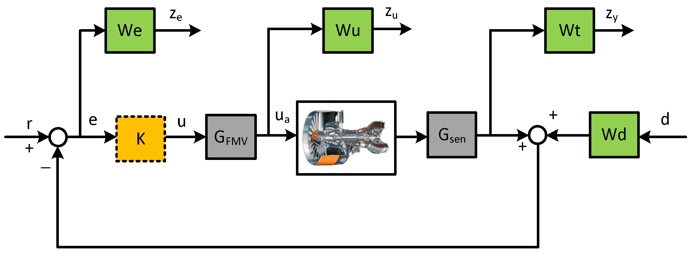
Next, the LPV controller will be designed based on the LPV model and simulated on the CLM of a dual-shaft turbofan engine. Figure 3 depicts the diagram of the interconnection structure of LPV control synthesis. $K$ denotes the controller. The dynamics of the fuel metering valve (FMV) are represented by $G_{FMV}$, which is the actuator of the aircraft engine. The dynamics of the low-pressure shaft speed sensor are denoted by $G_{sen}$. The actuator and sensor model are selected as first-order lag transfer functions with a unit gain and corresponding bandwidths of 20 rad/s and 50 rad/s, respectively. Signal d denotes the sensor noise and unmodeled dynamics of the aircraft engine. For the controller design of this simulation, the weighting functions are selected as $W_e=\frac{s/1000+1}{s/6+0.005}$, $W_t=\frac{1000s+8}{s+8000}$, and $W_d=\frac{s+0.3}{0.01s+20}$. In order to avoid an excessive order of the controller, we choose a constant control weighting $W_u=1$. Generally, the engine dynamics in Figure 3 are replaced by the CLM of a turbofan engine.

Due to the use of PDLF-based methods to solve LPV controllers in this paper, it is necessary for the designer to specify the basis functions for solving LMIs. Despite the importance of the basis function in solving LPV controllers, there is currently no systematic method for determining the basis functions. In this paper, we specify the basis functions as 1, $n_f$, and $n_f^2$. Furthermore, we set the upper and lower bound of the scheduling parameter derivative used by the PDLF method to ±700/s. And in this simulation, we choose the following two sub-regions in the flight envelope:

$$\begin{array}{l}{\mathrm{\Theta }}^{\left(c\right)}\times {\mathrm{\Theta }}^{\left(m\right)\left[1\right]}=\left\{0.42\le n_f\le 1\right\}\times \left\{Ma=0.4,1Km\le H\le 3Km\right\}\\ {\mathrm{\Theta }}^{\left(c\right)}\times {\mathrm{\Theta }}^{\left(m\right)\left[2\right]}=\left\{0.42\le n_f\le 1\right\}\times \left\{Ma=0.4,1.5Km\le H\le 3.5Km\right\}\end{array}$$

$\phi \left({\theta }^{\left(m\right)}\right)$, which, satisfying condition (30), is specified as

$$\phi \left({\theta }^{\left(m\right)}\right)=\{\begin{array}{ll}1,& \hspace{1em}1Km\le H\le 1.5Km\\ cos\frac{\pi \left(H-1.5\right)}{3},& \hspace{1em}1.5Km<H<3Km\\ 0,& \hspace{1em}3Km\le H\le 3.5Km\end{array}$$

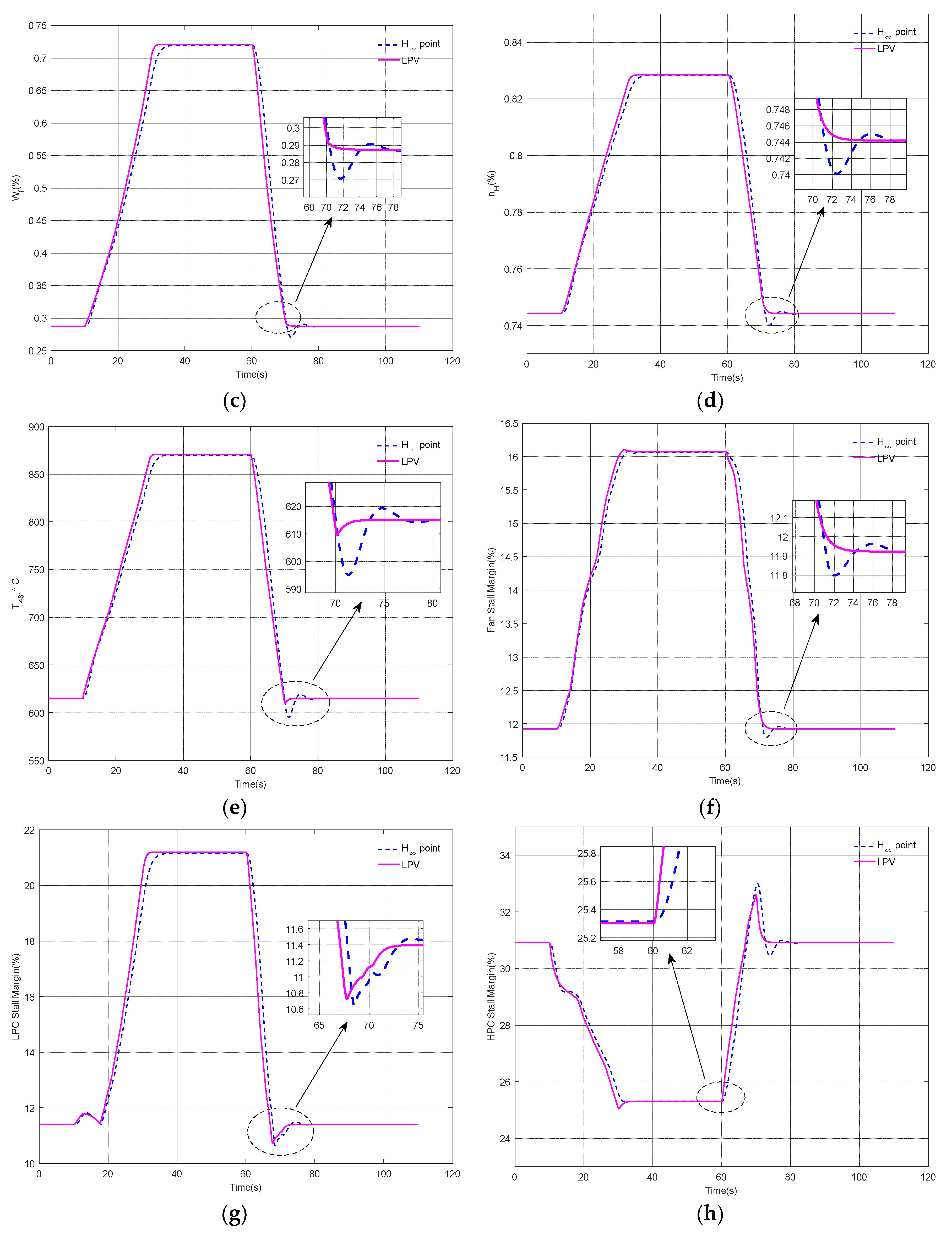
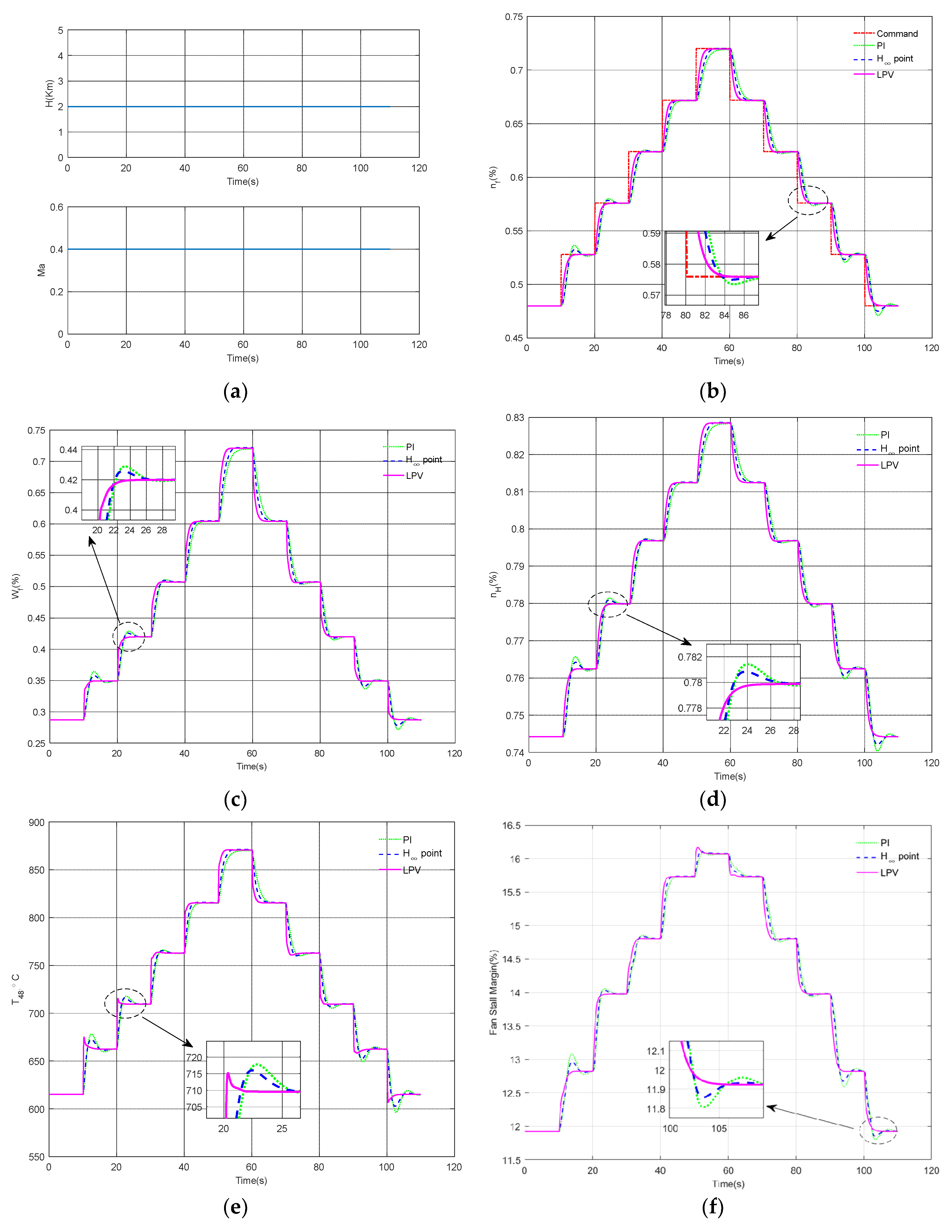
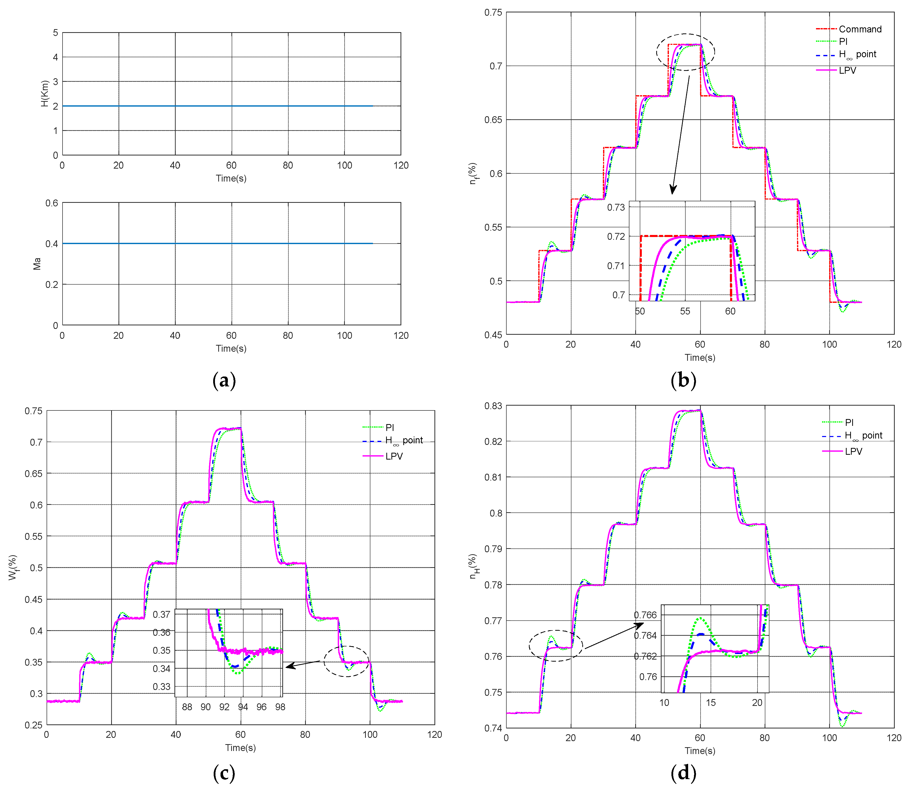
The simulation results are depicted in Figure 4, Figure 5, Figure 6 and Figure 7. Since the controlled variable used in this paper is the fan speed, it is necessary for $n_f$ to be specified as a command signal. In the CLM of aircraft engines, the flight altitude and Mach number are input parameters, and their values are specified by the designer. The transient characteristics of various engine variables for the stepped fan speed command under constant flight conditions are depicted in Figure 4. According to Figure 4a, the simulation of the engine is performed under flight conditions of H = 2 Km and Ma = 0.4. The simulation results of three control methods are compared, with green dotted lines, blue dashed lines, and magenta solid lines representing PI control, robust H_∞ point design, and LPV control methods, respectively. The red dash-dot line in Figure 4b represents the stepped fan speed command. As shown in Figure 4b, all three control methods can ensure that the given fan speed command can be tracked accurately and that the steady-state error is almost zero. However, compared to the other two methods, the transient characteristics of the fan speed using the LPV control method are smoother. In addition, locally enlarged Figure 4b,d verify that for frequently changing command signals, the dynamics of fan speed and high-pressure shaft speed using an LPV control design have a shorter rising time and no overshoot compared to the other two designs. In Figure 4e, although the total temperature response of the HPT outlet using the LPV control method shows overshoot, it is still smaller than the overshoot using the H_∞ point and PI control methods. And appropriately reducing the drastic temperature changes of engine turbine blades is helpful for extending the service life of the engine. Therefore, the LPV control method proposed in this paper can achieve a better transient performance than the H_∞ point design and PI design methods. The main reason is that more suitable engine inputs can be calculated by using the LPV control method; it can be seen in Figure 4c that the fuel flow transient by the LPV control design is smoother than that by the other two designs. Figure 4f–h provide the dynamic changes in the stall margin of three different components of the engine. For aircraft engine control, we hope that the stall margin of each component does not cross the stall boundary line during the acceleration or deceleration process of the engine to ensure safe operation. All three methods in Figure 4 can achieve this goal.

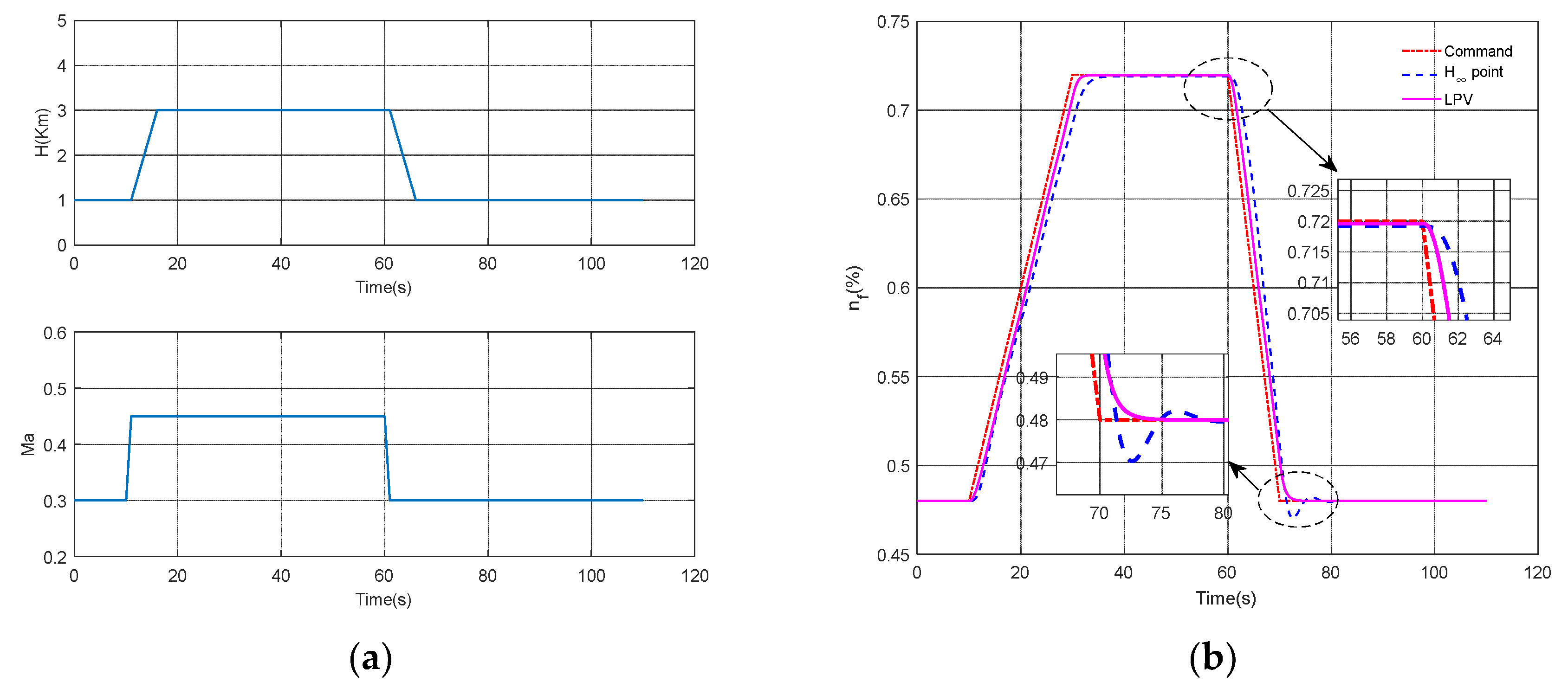
Figure 5 depicts the transient characteristics of various engine variables under varying flight conditions. The simulation of Figure 4 is performed under fixed flight conditions, and three design methods are compared. However, the simulation in Figure 5 is performed under variable flight conditions, and only the H_∞ point control and LPV control methods are compared. When flight conditions change, it is necessary to select more design points and repeatedly design a large number of PI controllers to achieve good control performance. In addition, the design of PI controllers also requires repeated parameter adjustments, which is very troublesome and greatly increases the workload. Therefore, the PI control design method is not used in the simulation of Figure 5. The changes in flight conditions are depicted in Figure 5a. Figure 5b indicates that the dynamic response speed of the fan speed using the LPV control method is faster than that using the H_∞ point control method in both the acceleration and deceleration stages. Moreover, Figure 5b–e show that compared to the H_∞ point control method, the response curve of the engine using the LPV control method does not have undershoot during the deceleration phase. The simulation in Figure 5 indicates that even for varying flight conditions, the LPV control method proposed in this paper can still provide a good transient performance while avoiding the cumbersome design of the H_∞ point control method.

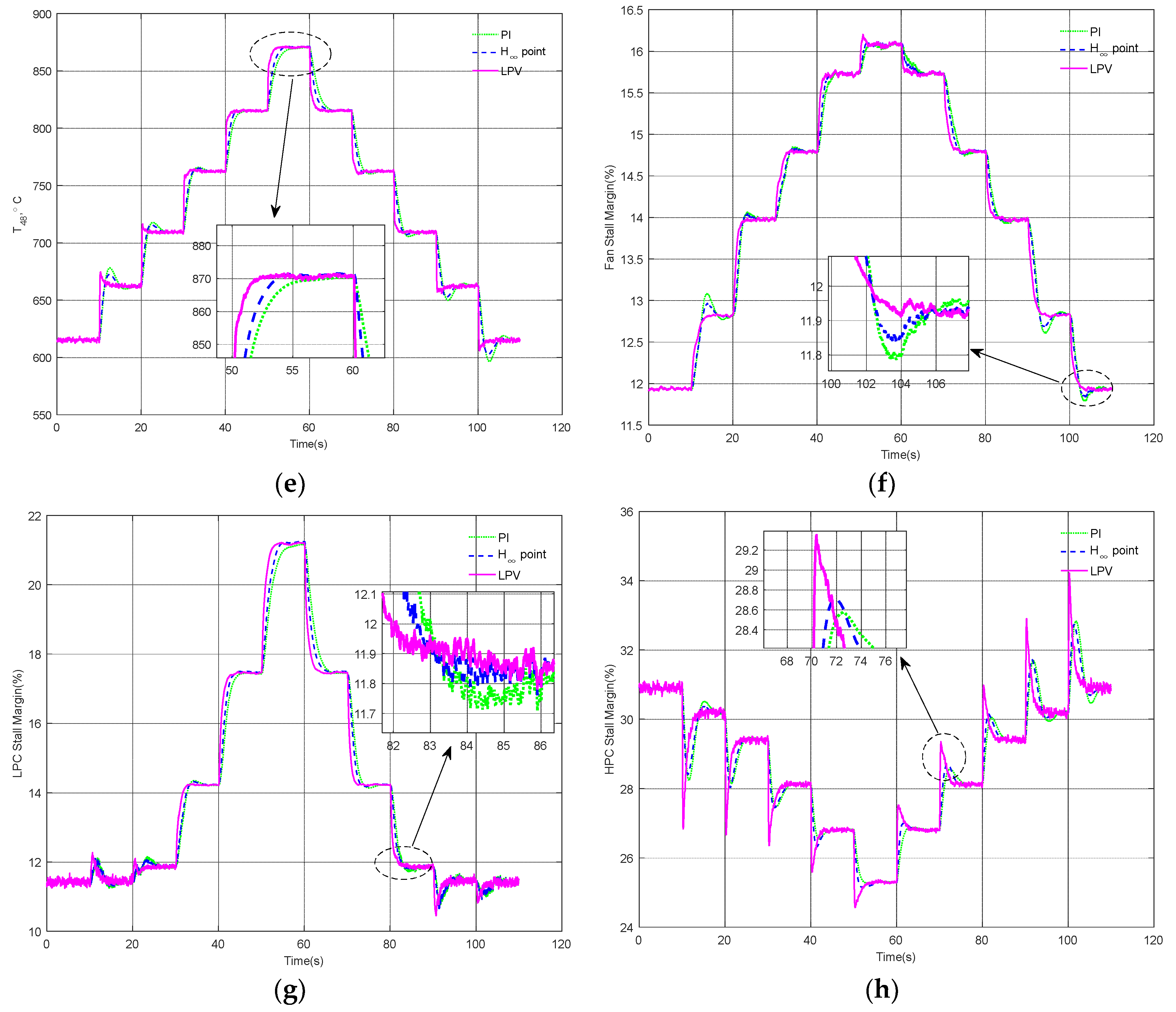
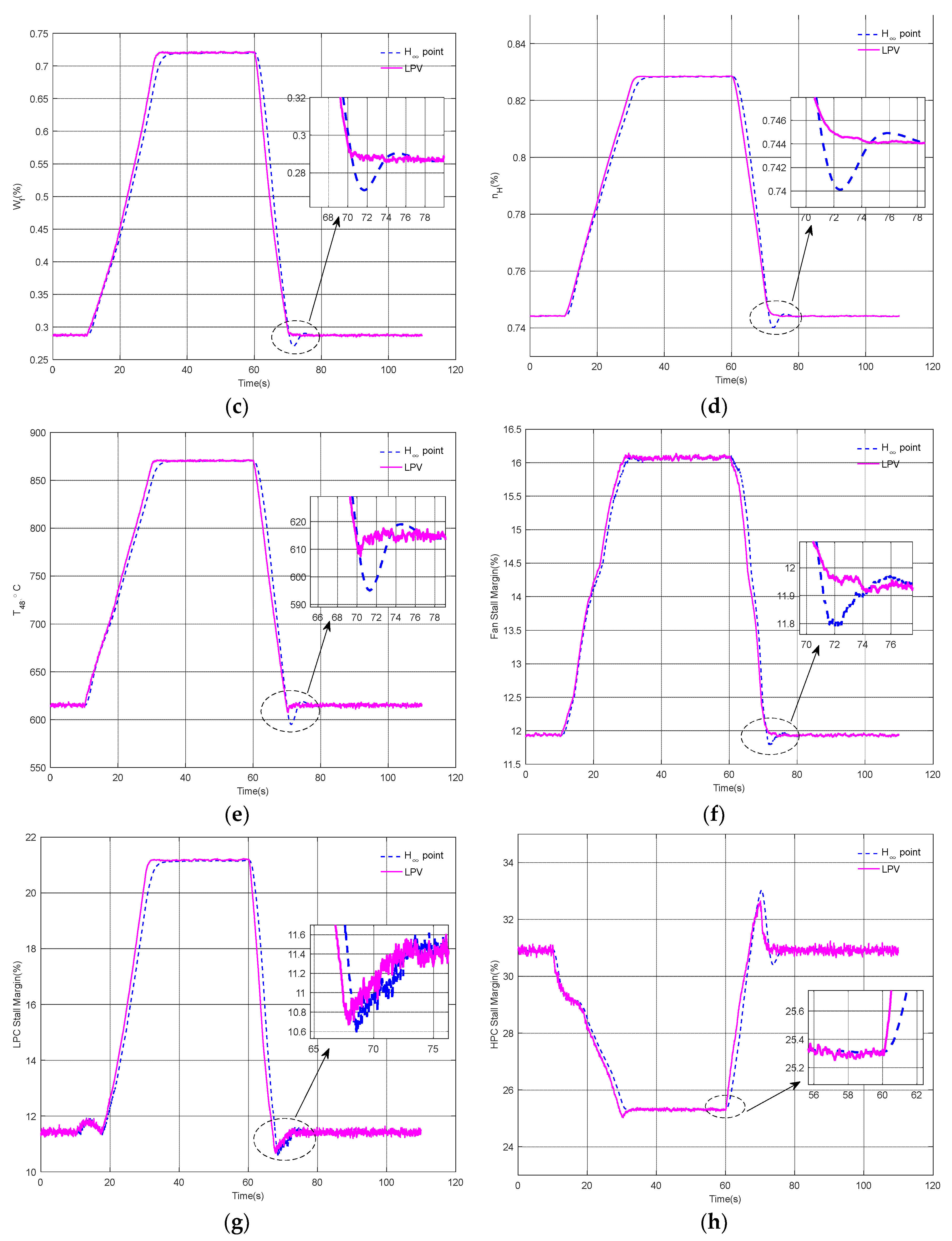
Next, the control performance of the system under sensor noise conditions will be verified. When the system is added to approximately 15% sensor noise, the simulation results of the engine under constant and variable flight conditions are described in Figure 6 and Figure 7, respectively. It is well known that the main goals of aircraft engine control include: accurate tracking of the fan speed with the reference command, no over-temperature of turbine blades, and no stall of three components (Fan, LPC, and HPC). In Figure 6 and Figure 7, all three methods can achieve these goals. The transient processes of Figure 6b,d and Figure 7b,d indicate that the responses of the fan speed and high-pressure shaft speed are insensitive to the sensor noise. From the locally enlarged Figure 6b,d and Figure 7b,d, it can be seen that the dynamic changes in the fan speed and high-pressure shaft speed using the LPV control method are smoother than those using other methods, including a faster response speed and smaller overshoot. This indicates that the LPV control method proposed in this paper is still effective even under sensor noise conditions. Figure 6c,e and Figure 7c,e indicate that, compared to other methods, although the fuel flow rate and HPT outlet total temperature using the LPV control method are slightly affected by the sensor noise, they still have a shorter settling time and smaller overshoot. Moreover, the total temperature response of the HPT outlet using all three methods did not show over-temperature. Figure 6f–h and Figure 7f–h verify that sensor noise has a large effect on the transient variations in the stall margin of the three engine components, especially the stall margin of LPC and HPC. Figure 6f,g and Figure 7f,g indicate that, compared to other methods, the transient responses of the stall margin of the fan and LPC using the LPV control method are slightly better. Although the transient responses of the HPC stall margin using the LPV control method in Figure 6h and Figure 7h are more affected by sensor noise compared to other methods, the HPC did not experience stall. In fact, the stall margin of the fan, LPC, and HPC are all unmeasurable variables, which are indirectly calculated through intermediate variables of the engine. The transient changes in the stall margin of the three components are insignificant as long as no stall occurs. Although all three methods in Figure 6 and Figure 7 can achieve the engine control objectives, compared to the other two methods, the LPV control method can provide better transient responses of the fan speed without the need for tedious and repetitive designs.

7. Conclusions

A full envelope LPV control method for aircraft engines has been proposed in this paper. By partitioning the scheduling parameter space, sub-region LPV controllers and overall region LPV controllers are designed, respectively. Three control methods, including LPV design, H_∞ point design, and PI design, have been used to compare the simulation of aircraft engine CLMs. The simulation results show that, using the proposed LPV control method, the dynamic characteristics of various engine variables have a better transient performance, including a shorter rise time and smaller overshoot. Even for varying flight conditions, the proposed method can still provide good control performance without the need for tedious and repetitive designs. In addition, the LPV control method proposed in this paper remains effective when approximately 15% of the sensor noise is added to the system.