Goodness–of–Fit Tests for Bivariate Time Series of Counts

Abstract

This article considers goodness-of-fit tests for bivariate INAR and bivariate Poisson autoregression models. The test statistics are based on an L2-type distance between two estimators of the probability generating function of the observations: one being entirely nonparametric and the second one being semiparametric computed under the corresponding null hypothesis. The asymptotic distribution of the proposed tests statistics both under the null hypotheses as well as under alternatives is derived and consistency is proved. The case of testing bivariate generalized Poisson autoregression and extension of the methods to dimension higher than two are also discussed. The finite-sample performance of a parametric bootstrap version of the tests is illustrated via a series of Monte Carlo experiments. The article concludes with applications on real data sets and discussion.

1. Introduction

Time series of counts enjoy numerous applications in such diverse fields as business, economics, engineering, and epidemiology, and corresponding inferential procedures have been intensively studied in recent years. The reader is referred to the earlier work of McKenzie (2003), as well as to the much updated full-book treatment of Davis et al. (2015) and Weiss (2018a) for an overview of the subject. Among the most popular models for count-time series are the integer autoregression (INAR) model and the Poisson autoregressive (PAR) model, also termed Poisson INARCH model. The INAR and PAR models, originally conceived for univariate counts, have been extended in order to accommodate bivariate, and more generally multivariate counts; see Latour (1997) and Liu (2012), respectively. One of the basic parametric elements of these generalizations involves moving from a univariate to a bivariate distribution, and eventually to a multivariate one.

In this connection, when confronted with a vectorial data-set of time series of counts, and since one is presented with a choice of several possible candidate models, it is extremely important to check model-adequacy via some goodness-of-fit (GOF) test. Otherwise a poorly fitted model might yield misleading inference. Various such procedures have been proposed in the literature for univariate series of counts. A brief overview of these approaches is provided in Section 2.

Inspired by the univariate test criteria, we propose GOF tests for bivariate INAR and PAR models. Our tests mainly target the (by far most popular) Poisson specification of these models, but also involve other structural aspects, such as order and functional specification of the underlying model. The suggested test statistic is constructed as a contrast between an estimator of the probability generating function (PGF) which is entirely model-free and a semiparametric counterpart that “respects” the model under test. Hence each new test may be viewed as a bivariate extension of the earlier PGF-based procedure suggested by Meintanis and Karlis (2014), Hudecová et al. (2015) and Schweer (2016).

The remainder of this work unfolds as follows. Section 2 provides a review of the models considered and of goodness-of-fit testing for univariate time series of counts. In Section 3 and Section 4 we introduce the bivariate models and the new test criteria. In Section 5 the asymptotic properties of the methods are investigated and resampling versions of the tests are proposed. An extension of one the tests to a more complicated model is discussed in Section 6. The finite-sample properties of the new criteria are studied by means of Monte Carlo methods in Section 7. Applications to real data sets are included in Section 8 while our final thoughts regarding the news methods and potential extensions thereof are summarized in Section 9. Proofs of asymptotics are provided in Appendix A.

2. Goodness-of-Fit Methods for Univariate Time Series of Counts

Many of the models for time series of low counts assume that conditionally on the past, the distribution of the current variable is fully specified by a family of laws indexed by a certain parameter. An important example is a class of integer autoregressive conditionally heteroscedastic (INGARCH) models, covering PAR models as special cases. Different models are based on the thinning operator see Steutel and van Harn (1979), with the INAR model being the most popular one. In the following, a count distribution refers to a discrete distribution on ${\mathbb{N}}_0=\mathbb{N}\cup \left\{0\right\}$ and a count variable is a random variable with such distribution.

Let $\left\{Y_t\right\}=\{Y_t,t\in \mathbb{Z}\}$ be a univariate time series and let ${\mathcal{F}}_t=\sigma \{Y_s,s\le t\}$ is the information known up to time t. An integer GARCH model, abbreviated as nonlinear INGARCH($p,q$), is defined as

$$Y_t|{\mathcal{F}}_{t-1}\sim F\left({\lambda }_t\right),{\lambda }_t=r(Y_{t-1},\cdots ,Y_{t-p},{\lambda }_{t-1},\cdots ,{\lambda }_{t-q},\mathit{\eta }),$$

(1)

where $F\left(\lambda \right)$ is some count distribution with mean $\lambda$, and the regression function $r:{[0,\infty )}^{p+q}\times \mathsf{\Theta }$ belongs to some specific parametric family of functions $\mathcal{R}=\{r(·,\mathit{\eta }):\mathit{\eta }\in \mathsf{\Theta }\subset {\mathbb{R}}^k\}$ for some $k\ge 1$. If F is Poisson and $\mathcal{R}$ is a family of linear functions then this model is referred to as Poisson (linear) INGARCH, see Ferland et al. (2006). Some authors also use the name Poisson autoregression for cases where F is Poisson and r could be nonlinear, see, e.g., Fokianos and Tjøstheim (2009), Fokianos and Tjøstheim (2012), Fokianos (2012), for the case $p=q=1$. If $q=0$ then the model has a purely autoregressive structure and is abbreviated as INARCH$\left(p\right)$. In the following the acronym PAR(p) is used for INARCH(p) with F Poisson and r linear. It has been shown that if $p=q=1$ and r is linear, i.e., $r(\mathbf{x},\mathit{\eta })={\eta }_1+{\eta }_2{x}_1+{\eta }_3{x}_2$, and if ${\eta }_i\ge 0$ and ${\eta }_2+{\eta }_3<1$ and F belongs to the single-parameter exponential family of distributions (that includes the Poisson distribution as a special case), then there exists a strictly stationary and ergodic solution of (1), see Davis and Liu (2016). For an overview of conditions for strict stationarity and ergodicity for other choices of F see e.g., (Ahmad and Francq 2016, Section 3).

A different class of models consists of integer autoregressive moving average (INARMA) models. These models arise from the same structure as the classical ARMA time series models, but the multiplication sign is replaced by the Steutel and van Harn’s thinning operator ∘. If Y is a count random variable and $\alpha \in (0,1)$ then

$$\alpha \circ Y:=\sum _{i=1}^Y{U}_i,$$

(2)

where $\left\{U_i\right\}$ are iid Bernoulli variables with $\alpha =𝖯(U_i=1)=1-𝖯(U_i=0)$, which are independent of Y, with the convention that an empty sum (the case $Y=0$) equals 0. Let $\left\{{\epsilon }_t\right\}$ be a sequence of iid count random variables with distribution G with a finite variance, and let ${\alpha }_i,{\beta }_j\in (0,1)$ for $i=1,\cdots ,p$, $j=1,\cdots ,q$. The INARMA$(p,q)$ model is defined as

$$Y_t=\sum _{i=1}^p{\alpha }_i\circ Y_{t-i}+{\epsilon }_t+\sum _{j=1}^q{\beta }_j\circ {\epsilon }_{t-j},$$

(3)

where the Bernoulli variables involved in all the thinning operations are independent and independent of $\left\{{\epsilon }_t\right\}$. If $p=1,q=0$ then the model (3) corresponds to the INAR(1) model introduced in McKenzie (1985) and Al-Osh and Alzaid (1987), taking the following form

$$Y_t=\alpha \circ Y_{t-1}+{\epsilon }_t=\sum _{i=1}^{Y_{t-1}}{U}_{t,i}+{\epsilon }_t.$$

(4)

For $\alpha \in (0,1)$ there exists a strictly stationary solution of (4) and the law of the innovations $\left\{{\epsilon }_t\right\}$ uniquely determines the marginal distribution of $Y_t$ as well as the conditional distribution $Y_t|{\mathcal{F}}_{t-1}$. In particular, if $\left\{{\epsilon }_t\right\}$ are iid Poisson then $Y_t$ has Poisson distribution as well, and this special case has been considered in many applications. Model (3) with $p>1$, $q=0$, was introduced and studied by Du and Li (1991) and since then, many authors have considered variants of model (3), various extensions and modifications, see Scotto et al. (2015) for a comprehensive review.

Various GOF tests have been suggested in the literature for the aforementioned two classes of models. Neumann (2011) and Fokianos and Neumann (2013) considered GOF tests for the regression function r in a Poisson INGARCH(1,1); see model (1) with $p=q=1$ and Poisson F. A slightly less formal assessment of model adequacy is explored in Aleksandrov and Weiss (2020) for a PAR(1) model as well as for a Poisson INAR(1). GOF tests based on the sample index of dispersion were considered in Schweer and Weiss (2014) and Weiss et al. (2019) for a Poisson INAR(1), and by Weiss and Schweer (2015) for a PAR(1). A test based on the classical Pearson’s ${\chi }^2$ statistic for the marginal distribution specified by the null hypothesis is proposed by Weiss (2018b) for a Poisson INAR(p).

A different approach to GOF testing for time series of counts is based on the probability generating function (PGF). Recall that if Y is a nonnegative discrete random variable then its PGF is defined as $g_Y\left(u\right)=\mathsf{E}{u}^Y$ for all u for which the expectation is finite, which is always the case for $u\in [0,1]$. The distribution of Y can be easily obtained from $g_Y^{\left(k\right)}\left(0\right)$ and thus the PGF uniquely determines the distribution of Y. If $\mathbf{Y}={(Y_1,Y_2)}^{\top }$ is a count random vector then its PGF is defined as $g_{\mathbf{Y}}\left(\mathbf{u}\right)=\mathsf{E}\left(u_1^{Y_1}{u}_2^{Y_2}\right)$ and exists for all $\mathbf{u}={(u_1,u_2)}^{\top }\in {[0,1]}^2$. Test criteria involving the estimates of the PGF of ${(Y_t,Y_{t-1})}^{\top }$ have proved as useful not only for assessing the specification of F in (1) or G in (4), but also for determination the model itself, see Meintanis and Karlis (2014) for INAR(1) and Schweer (2016) for a more general setup involving INAR(1) and PAR(1) as special cases. In both mentioned articles the considered test statistic is an integrated $L_2$ distance between the empirical PGF of ${(Y_t,Y_{t-1})}^{\top }$ and the parametric estimate of $g_{{(Y_t,Y_{t-1})}^{\top }}$ under the null hypothesis. Hudecová et al. (2015) also consider tests based on PGF, but instead of the estimator $g_{{(Y_t,Y_{t-1})}^{\top }}$, their criteria are constructed as an integrated $L_2$ distance between the nonparametric estimate ${\widehat{g}}_n\left(u\right)=n^{-1}{\sum }_{t=1}^n{u}^{Y_t}$ of the marginal PGF $g_Y$ and a semiparametric estimate of $g_Y$, which is model-specific. In the following sections we extend this approach from the univariate to the bivariate setup.

3. Bivariate Models for Time Series of Counts

The bivariate INAR and PAR models considered in this paper are based on the following bivariate distribution: We say that $\mathbf{Y}={(Y_1,Y_2)}^{\top }$ follows a bivariate Poisson distribution, see Kocherlakota and Kocherlakota (1992), denoted as $\mathsf{BP}({\lambda }_1,{\lambda }_2,\varphi )$, if its PGF is

$$g_{\mathbf{Y}}\left(\mathbf{u}\right)=exp\{{\lambda }_1(u_1-1)+{\lambda }_2(u_2-1)+\varphi (u_1-1)(u_2-1)\},\mathbf{u}\in {[0,1]}^2,$$

(5)

where ${\lambda }_1-\varphi >0,{\lambda }_2-\varphi >0,\varphi >0$. This distribution arises via the trivariate reduction method, i.e., $Y_1=U_1+U_2$, $Y_2=U_1+U_3$, where $U_1,U_2,U_3$ are independent with Poisson distribution with mean $\varphi ,{\lambda }_1-\varphi$, ${\lambda }_2-\varphi$ respectively.

The models based on this kind of bivariate Poisson distribution seem to be the most popular in the literature despite some of their limitations. Please note that a different construction of a bivariate distribution with Poisson marginals is considered in Lakshminarayana et al. (1999).

3.1. Bivariate INAR Model

Suppose that we have a time series $\left\{{\mathbf{Y}}_t\right\}$ composed by a pair of counts, i.e., ${\mathbf{Y}}_t:={(Y_{t,1},Y_{t,2})}^{\top }$. Following Latour (1997) we say that $\left\{{\mathbf{Y}}_t\right\}$ follows a bivariate INAR model of the first order, in the following referred to as BINAR, if

$${\mathbf{Y}}_t=\mathbf{A}\circ {\mathbf{Y}}_{t-1}+{\mathit{\epsilon }}_t,$$

(6)

where ${\mathit{\epsilon }}_t={({\epsilon }_{t,1},{\epsilon }_{t,2})}^{\top }$ are iid bivariate count random vectors with finite covariance matrix, $\mathbf{A}$ denotes a $2\times 2$ matrix with elements $a_{ij}$, $i,j=1,2$, and the operator ∘ is a multivariate generalization of (2). Namely the operator ∘ from (6) acts on a count random vector $\mathbf{Y}$ of dimension two by means of the equation

$$\mathbf{A}\circ \mathbf{Y}=\left(\begin{array}{c}{a}_{11}\circ Y_1+a_{12}\circ Y_2\\ a_{21}\circ Y_1+a_{22}\circ Y_2\end{array}\right),$$

where the univariate thinning operators was defined in (2).

Latour (1997) showed that if the spectral radius (the absolute value of the largest eigenvalue) of $\mathbf{A}$ is smaller than 1 and ${\mathit{\epsilon }}_t$ has a finite covariance matrix then there exists a strictly stationary and ergodic process satisfying (6). Furthermore, the conditional least squares (CLS) estimate is shown to be consistent and asymptotically normal. Maximum likelihood estimation is considered in Pedeli and Karlis (2011) and Pedeli and Karlis (2013c), with a special emphasis on the Poisson specification for ${\mathit{\epsilon }}_t$. For estimation of BINAR with negative Binomial innovations the reader is referred to Mamode Khan et al. (2019) and references therein.

3.2. Bivariate PAR Model

Let ${\mathcal{F}}_t=\sigma \{{\mathbf{Y}}_s,s\le t\}$. We say that $\left\{{\mathbf{Y}}_t\right\}$ follows a bivariate Poisson autoregression model of the first order, referred to as BPAR, model if,

$${\mathbf{Y}}_t|{\mathcal{F}}_{t-1}\sim \mathsf{BP}({\lambda }_{t,1},{\lambda }_{t,2},\varphi ),{\mathit{\lambda }}_t=\left(\begin{array}{c}{\lambda }_{t,1}\\ {\lambda }_{t,2}\end{array}\right)=\underset{\alpha }{\underbrace{\left(\begin{array}{c}{\alpha }_1\\ {\alpha }_2\end{array}\right)}}+\underset{\mathbf{B}}{\underbrace{\left(\begin{array}{cc}{b}_{11}& b_{12}\\ b_{21}& b_{22}\end{array}\right)}}\left(\begin{array}{c}{Y}_{t-1,1}\\ Y_{t-1,2}\end{array}\right),$$

(7)

where ${\alpha }_1,{\alpha }_2\ge 0$ and the matrix $\mathbf{B}$ has non-negative entries and is of full-rank. This model is sometimes referred to as a bivariate Poisson INARCH(1) model, e.g., Lee et al. (2018). Liu (2012) proved that if $2^{1-1/p}{\parallel \mathbf{B}\parallel }_p<1$ for some $1\le p\le \infty$ then $\{{\mathbf{Y}}_t,{\mathit{\lambda }}_t\}$ is strictly stationary and ergodic, with ${\parallel \mathbf{B}\parallel }_p={sup}_{\mathbf{x}\ne 0,\mathbf{x}\in {\mathbb{C}}^2}{\parallel \mathbf{B}\mathbf{x}\parallel }_p/{\parallel \mathbf{x}\parallel }_p.$ Strong consistency of the conditional maximum likelihood estimator (CMLE) of parameters was proved by Andreassen (2013) under the extra assumption $\varphi <min\{{\alpha }_1,{\alpha }_2\}$, while Lee et al. (2018) further showed that the CMLE has an asymptotic normal distribution.

4. Goodness-of-Fit Tests

Assume that we have observations ${\mathbf{Y}}_1,\cdots ,{\mathbf{Y}}_n$, which come from a stationary bivariate time series of counts and we would like to perform a GOF test to a particular model for this data, with the model being fixed apart from finite-dimensional parameters. Let $\upsilon (·,·)$ be a non-negative weight function which will be further specified below. We propose as test statistic the weighted distance measure

$$S_{n,\upsilon }=n{\int }_0^1{\int }_0^1{[{\widehat{g}}_n(u_1,u_2)-{\widehat{g}}_{n,0}(u_1,u_2)]}^2\upsilon (u_1,u_2)\mathrm{d}{u}_1\mathrm{d}{u}_2,$$

(8)

where ${\widehat{g}}_n(u_1,u_2)$ is a non-parametric estimate of $g_{\mathbf{Y}}(u_1,u_2)$ based on ${\mathbf{Y}}_1,\cdots ,{\mathbf{Y}}_n$, given by ${\widehat{g}}_n(u_1,u_2)=n^{-1}{\sum }_{t=1}^n{u}_1^{Y_{t,1}}{u}_2^{Y_{t,2}}$ and where ${\widehat{g}}_{n,0}(u_1,u_2)$ is a semi-parametric estimate of the PGF $g_{\mathbf{Y}}(u_1,u_2)$ of $\mathbf{Y}$, which is constructed specifically under the model being tested. The null hypothesis is rejected for large values of $S_{n,\upsilon }$.

By analogy to most, if not all, of the previously published work we consider $\mathbf{u}\in {[0,1]}^2$ as our working interval, despite the fact that uniqueness of PGFs and corresponding consistency of the test might require working on a region of $\mathbf{u}$ containing the origin. Nevertheless we further investigate this aspect of our tests by simulations. See Esquível (2008) for a recent account of uniqueness of PGFs.

Although the idea of the proposed test statistics is analogous as for the univariate models mentioned in Section 2, the extension to a bivariate case is not straightforward, neither in terms of asymptotics nor on computational grounds as the multivariate nature of the data brings in some elevated technical difficulties. We state the necessary assumptions and provide a formal proof for the asymptotics of the suggested test statistic. In addition, extension of our GOF tests to more complex models is briefly discussed. In fact, and although here we only treat the bivariate case, extension to higher dimension also comes completely natural with our methods.

4.1. Tests for the BINAR Model

Let $\mathcal{G}=\{g_{\epsilon }(·;\mathit{\theta }):\mathit{\theta }\in \mathsf{\Theta }\}$ denote a parametric family of PGFs indexed by a parameter $\theta \in \mathsf{\Theta }$, with $\mathsf{\Theta }$ being a compact subset of ${\mathbb{R}}^k$, $k\in \mathbb{N}$. We would like to test the null hypothesis

$$\begin{array}{cc}\hfill {\mathcal{H}}_0:& \left\{{\mathbf{Y}}_t\right\}\mathrm{follows}\mathrm{model}\left(6\right)\mathrm{for}\mathrm{some}\mathrm{sequence}{\mathit{\epsilon }}_t\mathrm{with}\mathrm{PGF}\mathrm{in}\mathcal{G}.\hfill \end{array}$$

Assume that $\left\{{\mathbf{Y}}_t\right\}$ is strictly stationary with PGF $g_{\mathbf{Y}}$. Then it follows from the properties of BINAR that

$$\begin{array}{cc}\hfill g_{\mathbf{Y}}(u_1,u_2)& =\mathsf{E}\left(u_1^{Y_{t,1}}{u}_2^{Y_{t,2}}\right)=\mathsf{E}\left(\mathsf{E}\left(u_1^{Y_{t,1}}{u}_2^{Y_{t,2}}|{\mathcal{F}}_{t-1}\right)\right)\hfill \\ \hfill & =g_{\mathit{\epsilon }}(u_1,u_2;\mathit{\theta })·g_{\mathbf{Y}}(w_{11}{w}_{21},w_{12}{w}_{22}),\hfill \end{array}$$

(9)

where

$$w_{ij}=w_{ij}(\mathbf{u},\mathbf{a})=1+a_{ij}(u_i-1),$$

and $\mathbf{a}:=\mathsf{vec}\left(\mathbf{A}\right)={(a_{11},a_{21},a_{12},a_{22})}^{\top }$ denotes the vectorized version of $\mathbf{A}$.

Here we used the fact that for a Binomial distribution with parameters $(m,p)$ the PGF is ${(1+p(u-1))}^m$, so that if additionally $\widehat{\mathbf{a}}$ and $\widehat{\mathit{\theta }}$ are suitable estimators of the unknown parameters, then (9) yields a semi-parametric estimate of $g_{\mathbf{Y}}$ under model (6) as

$${\widehat{g}}_{n,0}(u_1,u_2)=g_{\epsilon }(\mathbf{u},\widehat{\mathit{\theta }}){\widehat{g}}_n({\widehat{w}}_{11}{\widehat{w}}_{21},{\widehat{w}}_{12}{\widehat{w}}_{22}),$$

(10)

where ${\widehat{w}}_{ij}=w_{ij}(\mathbf{u},\widehat{\mathbf{a}})$.

We will consider a GOF test for the null hypothesis ${\mathcal{H}}_0$ with $\mathcal{G}$ being the family of bivariate Poisson distributions with unspecified parameters. Interest in testing ${\mathcal{H}}_0$ lies in the fact that while this distribution is by far the most popular in the univariate as well as in the multivariate context, alternative specifications have also been employed such as models with innovations following a bivariate negative Binomial distribution; see for instance Pedeli and Karlis (2013a), Popović et al. (2018), and Kim and Lee (2017). Also BPAR models (see next section) may be considered to be alternative models of interest.

4.2. Tests for the BPAR Model

The corresponding null hypothesis for the BPAR model is formulated as

$${\tilde{\mathcal{H}}}_0:\left\{{\mathbf{Y}}_t\right\}\mathrm{follows}\mathrm{model}\left(7\right).$$

If $\left\{{\mathbf{Y}}_t\right\}$ is strictly stationary, then it follows from the properties of the model that the PGF of ${\mathbf{Y}}_t$ is given by

$$\begin{array}{cc}\hfill g_{\mathbf{Y}}(u_1,u_2)=& \mathsf{E}\left(u_1^{Y_{t,1}}{u}_2^{Y_{t,2}}\right)=\mathsf{E}\left(\mathsf{E}\left(u_1^{Y_{t,1}}{u}_2^{Y_{t,2}}\right|{\mathcal{F}}_{t-1})\right)\hfill \\ \hfill & =\mathsf{E}\left(exp\{{\lambda }_{t,1}(u_1-1)+{\lambda }_{t,2}(u_2-1)+\varphi (u_1-1)(u_2-1)\}\right)\hfill \\ \hfill & ={\mathrm{e}}^{\varphi (u_1-1)(u_2-1)+{\alpha }_1(u_1-1)+{\alpha }_2(u_2-1)}\hfill \\ \hfill & \times \mathsf{E}\left({\mathrm{e}}^{Y_{t-1,1}[b_{11}(u_1-1)+b_{12}(u_2-1)]}{\mathrm{e}}^{Y_{t-1,2}[b_{21}(u_1-1)+b_{22}(u_2-1)]}\right)\hfill \end{array}$$

(11)

$$\begin{array}{cc}\hfill & ={\mathrm{e}}^{\varphi (u_1-1)(u_2-1)+{\alpha }_1(u_1-1)+{\alpha }_2(u_2-1)}{g}_{\mathbf{Y}}(w_1,w_2),\hfill \end{array}$$

(12)

where

$$w_i={\mathrm{e}}^{b_{1i}(u_1-1)+b_{2i}(u_2-1)},i=1,2.$$

(13)

Thus, if we have an appropriate estimator $\widehat{\mathit{\theta }}$ of the parameter $\mathit{\theta }:={({\mathit{\alpha }}^{\top },\mathsf{vec}\left(\mathbf{B}\right),\varphi )}^{\top }={({\alpha }_1,{\alpha }_2,b_{11},b_{21},b_{12},b_{22},\varphi )}^{\top }$, then in view of (11) we may define a semi-parametric estimate of $g_{\mathbf{Y}}$ as

$$\begin{array}{c}\hfill {\widehat{g}}_{n,0}(u_1,u_2)=e^{\widehat{\varphi }(u_1-1)(u_2-1)+{\widehat{\alpha }}_1(u_1-1)+{\widehat{\alpha }}_2(u_2-1)}{\widehat{g}}_n({\widehat{w}}_1,{\widehat{w}}_2):=c(\mathbf{u},\widehat{\mathit{\theta }}){\widehat{g}}_n({\widehat{w}}_1,{\widehat{w}}_2),\end{array}$$

(14)

where

$${\widehat{w}}_i=e^{{\widehat{b}}_{1i}(u_1-1)+{\widehat{b}}_{2i}(u_2-1)},$$

and

$$c(\mathbf{u},\mathit{\theta })=e^{\varphi (u_1-1)(u_2-1)+{\alpha }_1(u_1-1)+{\alpha }_2(u_2-1)}.$$

(15)

Deviations from the null hypothesis ${\tilde{\mathcal{H}}}_0$ include non-Poisson conditionals (see Heinen and Rengifo (2007)) as well as model violations towards more general specifications.

Remark 1.

We should remark that the tests proposed in this article are not for BINAR or BPAR models per se. Specifically the test criterion for BINAR is for bivariate counts for which the PGF satisfies Equation (9), and analogously the test criterion for BPAR is for bivariate counts for which the PGF satisfies Equation (12). In the context of time series of counts however, BINAR and BPAR models are framed by Equations (9) and (12), respectively, to such an extend that for all practical purposes these equations may be regarded as characterizing equations for the models themselves. Thus, our tests could be viewed as being on an equal footing with universally consistent methods such as those suggested by Fokianos and Neumann (2013), Jiménez-Gamero et al. (2020), and Leucht et al. (2015).

4.3. Computations

From (8) and by means of (10) and (14), we have after straightforward algebra

$$S_{n,\upsilon }=\frac{1}{n}\sum _{i=1}^n\sum _{j=1}^n{\Delta }_{i,j},$$

where ${\Delta }_{i,j}=\Delta ({\mathbf{Y}}_i,{\mathbf{Y}}_j)$ with

$$\begin{array}{c}\hfill {\Delta }_{i,j}={\int }_0^1{\int }_0^1{D}_i(u_1,u_2)D_j(u_1,u_2)\upsilon (u_1,u_2)\mathrm{d}{u}_1\mathrm{d}{u}_2\end{array}$$

(16)

where

$$D_i(u_1,u_2)=u_1^{Y_{i,1}}{u}_2^{Y_{i,2}}-g_{\epsilon }(u_1,u_2;\widehat{\theta }){\left({\widehat{w}}_{11}{\widehat{w}}_{21}\right)}^{Y_{i,1}}{\left({\widehat{w}}_{12}{\widehat{w}}_{22}\right)}^{Y_{i,2}},$$

for the BINAR model, and

$$D_i(u_1,u_2)=u_1^{Y_{i,1}}{u}_2^{Y_{i,2}}-c(\mathbf{u},\widehat{\mathit{\theta }}){\widehat{w}}_1^{Y_{i,1}}{\widehat{w}}_2^{Y_{i,2}},$$

for the BPAR model.

The integral figuring in Equation (16) with weight function $\upsilon (u_1,u_2)=u_1^{\gamma }{u}_2^{\gamma },\gamma \ge 0$, may be expressed in more elementary terms. However the final fully reduced explicit forms, which are available from the authors upon request, are not convenient from the computational point of view. Thus, the tests were implemented by numerical evaluation of the corresponding integrals.

5. Asymptotics

In this section, we study the asymptotic distribution of the test statistic $S_{n,\upsilon }$ under the null hypothesis of a BINAR model as well as the corresponding limit null distribution under a BPAR model. Results for the behavior under fixed alternatives are also provided and show that in both cases the test is consistent against certain fixed alternatives. Finally resampling versions are proposed that circumvent the problem of unknown components in the aforementioned limit null distributions. Please note that under the standing assumptions these results are valid for general innovation distribution and weight function as well as for arbitrary parameter-estimates.

5.1. Asymptotics of the Test Statistic: BINAR Case

Assume the test statistic $S_{n,\upsilon }$ (8) is constructed for testing ${\mathcal{H}}_0$ with specified $\mathcal{G}=\{g_{\epsilon }(·;\mathit{\theta }):\mathit{\theta }\in \mathsf{\Theta }\}$, for a compact $\mathsf{\Theta }$, i.e., the semi-parametric estimate ${\widehat{g}}_{n,0}$ is constructed by (10). Consider the following assumptions:

(A.1)

Let $\upsilon (·,·)$ be a non-negative function satisfying $0<{\int }_0^1{\int }_0^1\upsilon (u_1,u_2)\mathrm{d}{u}_1\mathrm{d}{u}_2<\infty$.

(A.2)

Let $\left\{{\mathbf{Y}}_t\right\}$ follow model (6), where the spectral radius of $\mathbf{A}$ is smaller than 1.

(A.3)

Let $\mathcal{G}$ correspond to distributions with finite second moment. Furthermore, let the second partial derivatives of $g_{\mathit{\epsilon }}$ with respect to $\mathit{\theta }$ exist and be continuous in $\theta$ and suppose that

$$\begin{array}{cc}\hfill \underset{\mathbf{u}\in {[0,1]}^2,\mathit{\theta }\in \mathsf{\Theta }}{sup}\left|\frac{\partial g_{\mathit{\epsilon }}}{\partial {\theta }_i}(\mathbf{u},\mathit{\theta })\right|& <\infty ,\hfill \\ \hfill \underset{\mathbf{u}\in {[0,1]}^2,\mathit{\theta }\in \mathsf{\Theta }}{sup}\left|\frac{\partial }{\partial u_i}\frac{\partial g_{\mathit{\epsilon }}}{\partial {\theta }_j}(\mathbf{u},\mathit{\theta })\right|& <\infty ,\hfill \\ \hfill {\int }_{{[0,1]}^2}\left|\frac{{\partial }^2{g}_{\epsilon }}{\partial {\theta }_i\partial {\theta }_j}(\mathbf{u},\mathit{\theta })\right|\upsilon \left(\mathbf{u}\right)\mathrm{d}\mathbf{u}& <\infty \hfill \end{array}$$

hold true for all $\mathit{\theta }\in \mathsf{\Theta }$ and $i,j\in \{1,\cdots ,k\}$, where (recall) that k is the dimension of $\mathit{\theta }$.

(A.4)

Let $\widehat{\mathit{\zeta }}:={({\widehat{\mathit{\theta }}}^{\top },{\widehat{\mathbf{a}}}^{\top })}^{\top }$ be an estimator of $\mathit{\zeta }:={({\mathit{\theta }}^{\top },{\mathbf{a}}^{\top })}^{\top }$ such that for some $q\ge 1$

$$\sqrt{n}(\widehat{\mathit{\zeta }}-\mathit{\zeta })=\frac{1}{\sqrt{n}}\sum _{t=q+1}^n\mathbf{l}({\mathbf{Y}}_t,{\mathbf{Y}}_{t-1},\cdots ,{\mathbf{Y}}_{t-q},\zeta )+o_P\left(1\right),$$

where ${\mathbf{l}}_t=\mathbf{l}({\mathbf{Y}}_t,{\mathbf{Y}}_{t-1},\cdots ,{\mathbf{Y}}_{t-q},\mathit{\zeta })={({\mathbf{l}}_{t,1}^{\top },{\mathbf{l}}_{t,2}^{\top })}^{\top }$ form a strictly stationary and ergodic sequence of martingale differences with finite variance. Here, ${\mathbf{l}}_{t,1}$ is of the same dimension as $\mathit{\theta }$ and ${\mathbf{l}}_{t,2}$ has the dimension of $\mathsf{vec}\left(\mathbf{A}\right)$, i.e., four.

Under (A.2) and (A.3), $\left\{{\mathbf{Y}}_t\right\}$ is strictly stationary and ergodic with finite second order moments, see Franke and Rao (1995). Regarding possible estimators $\widehat{\mathit{\zeta }}$ in (A.4), Franke and Rao (1995) considered the CMLE and proved its asymptotic normality under a set of regularity conditions. These conditions involve the finiteness of $\mathsf{E}\left(\parallel {\mathit{\epsilon }}_t{\parallel }^3\right)$ and some further assumptions on the distribution of ${\mathit{\epsilon }}_t$.

Theorem 1.

Under (A.1)–(A.4) and as $n\to \infty$, the limit distribution of $S_{n,\upsilon }$ under the null hypothesis ${\mathcal{H}}_0$ is the same as the distribution of

$${\int }_{{[0,1]}^2}{Q}^2(\mathbf{u},\mathit{\zeta })\upsilon \left(\mathbf{u}\right)\mathrm{d}\mathbf{u},$$

where $\{Q(\mathbf{u},\mathit{\zeta }),\mathbf{u}\in {[0,1]}^2\}$ is a Gaussian random field with zero mean and covariance structure

$$\begin{array}{cc}\hfill \mathsf{E}\left(Q\right(\mathbf{u},\mathit{\zeta })& Q(\mathbf{v},\mathit{\zeta }))\hfill \\ \hfill =& \mathsf{E}\left(\right[u_1^{Y_{q+1,1}}{u}_2^{Y_{q+1,2}}-g_{\mathit{\epsilon }}(\mathbf{u},\mathit{\theta })W_q(\mathbf{u},\mathbf{a})-{\mathbf{l}}_{q+1,1}{\left(\mathit{\zeta }\right)}^{\top }{h}_2(\mathbf{u},\mathit{\zeta })-{\mathbf{l}}_{q+1,2}{\left(\mathit{\zeta }\right)}^{\top }{h}_3(\mathbf{u},\mathit{\zeta })]\hfill \\ \hfill & \times [v_1^{Y_{q+1,1}}{v}_2^{Y_{q+1,2}}-g_{\mathit{\epsilon }}(\mathbf{v},\mathit{\theta })W_q(\mathbf{v},\mathbf{a})-{\mathbf{l}}_{q+1,1}{\left(\mathit{\zeta }\right)}^{\top }{h}_2(\mathbf{v},\mathit{\zeta })-{\mathbf{l}}_{q+1,2}{\left(\mathit{\zeta }\right)}^{\top }{h}_3(\mathbf{v},\mathit{\zeta })]),\hfill \end{array}$$

where ${\mathbf{l}}_{q+1,1}$ and ${\mathbf{l}}_{q+1,2}$ are from assumption (A.4) and

$$\begin{array}{cc}\hfill W_t(\mathbf{u},\mathbf{a})& =\prod _{i,j=1}^2{w}_{ij}{(\mathbf{u},\mathbf{a})}^{Y_{t,j}},\hfill \\ \hfill h_2(\mathbf{u},\mathit{\zeta })& ={\nabla }_{\theta }{g}_{\mathit{\epsilon }}(\mathbf{u},\mathit{\theta })g_{\mathbf{Y}}(w_{11}{w}_{21},w_{12}{w}_{22}),\hfill \\ \hfill h_3(\mathbf{u},\zeta )& =g_{\mathit{\epsilon }}(\mathbf{u},\mathit{\theta })\mathsf{E}\left({\nabla }_{\mathbf{a}}{W}_1(\mathbf{u},\mathbf{a})\right).\hfill \end{array}$$

The proof of the assertion is postponed to the Appendix A.

The asymptotic distribution of the test statistic $S_{n,\upsilon }$ depends on several unknown quantities. One possibility is to generate the Gaussian random field figuring in Theorem 1 with the theoretical quantities replaced by some consistent estimators and then compute the critical values. Another possibility is the parametric bootstrap, which is quite natural here. The justification of the bootstrap approximation under the null hypothesis proceeds along similar lines as the proof of Theorem 1, conducted conditionally on the observed data ${\mathbf{Y}}_1,\cdots ,{\mathbf{Y}}_n$ and with the help of assertions for triangular arrays and sums of martingale difference arrays.

Write $S_n:=S_n({\mathbf{Y}}_1,\cdots ,{\mathbf{Y}}_n;\widehat{\mathbf{\zeta }})$ for the test statistic based on the original observations ${\mathbf{Y}}_1,\cdots ,{\mathbf{Y}}_n$, and the resulting parameter estimate $\widehat{\mathbf{\zeta }}$. (Here for simplicity we suppress the dependence of $S_{n,\upsilon }$ on the weight function $\upsilon (·,·)$).

• Generate ${\mathit{\epsilon }}_t^{\ast },t=1,\dots n$, where ${\mathit{\epsilon }}_t^{\ast }$ are iid and follow the distribution with PGF $g_{\mathit{\epsilon }}(u,\widehat{\mathit{\theta }})$.
• Compute pseudo-observations ${\mathbf{Y}}_t^{\ast },t=1,\dots n$, using Equation (6) with ${\mathit{\epsilon }}_t$ replaced by ${\mathit{\epsilon }}_t^{\ast },t=1,\dots n$, and $\mathbf{A}$ replaced by $\widehat{\mathbf{A}}$.
• Fit the model (6) using ${\mathbf{Y}}_1^{\ast },\cdots ,{\mathbf{Y}}_n^{\ast }$, and compute the bootstrap estimator ${\widehat{\mathit{\zeta }}}^{\ast }$ of $\mathit{\zeta }$.
• Compute the corresponding test statistic $S_n^{\ast }:=S_n({\mathbf{Y}}_1^{\ast },\cdots ,{\mathbf{Y}}_n^{\ast };{\widehat{\mathit{\zeta }}}^{\ast })$.
• Repeat steps 1–4 several times, say B, and obtain the sequence of test statistics, $S_{1,n}^{\ast },\cdots ,S_{\mathrm{B},n}^{\ast }$.
• Compute the p-value as $(\#b:S_{b,n}^{\ast }\ge S_n)/\left(\mathrm{B}+1\right)$.

Next we shortly discuss the limit behavior of the test statistic under alternatives of type $g_{\mathit{\epsilon }}\notin \mathcal{G}$. We assume that model (6) holds true but $g_{\mathit{\epsilon }}$ in the null hypothesis ${\mathcal{H}}_0$ does not belong to $\mathcal{G}$. Moreover suppose that the estimators ${({\widehat{\mathit{\theta }}}^{\top },{\widehat{\mathbf{a}}}^{\top })}^{\top }$ satisfy

$${({\widehat{\theta }}^{\top },{\widehat{\mathbf{a}}}^{\top })}^{\top }\stackrel{𝖯}{\to }{({\theta }_{\mathbf{A}}^{\top },{\mathbf{a}}_{\mathbf{A}}^{\top })}^{\top },$$

(17)

for some ${\mathit{\theta }}_{\mathbf{A}}\in \mathsf{\Theta }$ and some ${\mathbf{a}}_{\mathbf{A}}$ such that the largest eigenvalue of the respective matrix ${\mathbf{A}}_{\mathbf{A}}$ is in absolute value smaller then 1.

Theorem 2.

Let $\left\{{\mathit{Y}}_t\right\}$ be strictly stationary with PGF $g_A(u_1,u_2)$ that is continuous in $(u_1,u_2)\in {[0,1]}^2$ and let $g_{\epsilon }(\mathit{u},\mathit{\theta })$ be continuous in θ. Let (A.1) and (17) be satisfied. Then, as $n\to \infty$,

$$\frac{S_{n,v}}{n}\stackrel{𝖯}{\to }{\int }_{{[0,1]}^2}{\left\{g_A\left(\mathbf{u}\right)-g_{\epsilon }(\mathbf{u},{\mathit{\theta }}_A)g_A(w_{11,A}{w}_{21,A},w_{12,A}{w}_{22,A})\right\}}^{2}v\left(\mathbf{u}\right)d\mathbf{u},$$

(18)

where $w_{ij,A}=w_{ij}(\mathbf{u},{\mathbf{a}}_A),i,j=1,2$.

The proof is omitted since it suffices to follow the line of proof of Theorem 1 and use stationarity and ergodicity of $\left\{{\mathbf{Y}}_t\right\}$.

The right-hand side of (18) is strictly positive unless the true PGF $g_{\epsilon }(·)$ coincides with the PGF $g_{\epsilon }(·;{\mathit{\theta }}_{\mathbf{a}})$ from the null hypothesis ${\mathcal{H}}_0$. This fact and the uniqueness of the PGF implies the consistency of the test which rejects the null hypothesis ${\mathcal{H}}_0$ for large values of the test statistic $S_{n,v}$ under such fixed alternatives. The test is also consistent for other types of fixed alternatives, e.g., against model violation. This feature of the test is further illustrated by Monte Carlo simulations in Section 7.

Please note that the test even has (non-negligible) power for some local alternatives, i.e., when the difference $g_{\epsilon }\left(u\right)-g_{\epsilon }(\mathit{u};{\mathit{\theta }}_{\mathbf{a}})$ tends to 0 not too fast as $n\to \infty$ and $g_{\mathit{\epsilon }}\left(\mathbf{u}\right)$ depends on n. However, a rigorous proof of this result is quite technical, and therefore it is not discussed here any further.

5.2. Asymptotics of the Test Statistic: BPAR Case

This section considers the problem of testing the BPAR model. Recall that $\mathit{\theta }={({\alpha }_1,{\alpha }_2,b_{11},\cdots ,b_{22},\varphi )}^{\top }$ stands for the vector of the parameters of the model (7), and suppose that:

(B.1)

The series $\left\{{\mathbf{Y}}_t\right\}$ is strictly stationary solution of (7) with parameters $\mathit{\theta }\in \mathsf{\Theta }$ such that $\varphi <min\{{\alpha }_1,{\alpha }_2\}$ and $\mathsf{\Theta }$ is compact.

(B.2)

The estimator $\widehat{\mathit{\theta }}$ of the parameter $\mathit{\theta }$ is such that

$$\sqrt{n}(\widehat{\mathit{\theta }}-\mathit{\theta })=\frac{1}{\sqrt{n}}\sum _{t=q+1}^n\mathbf{l}({\mathbf{Y}}_t,{\mathbf{Y}}_{t-1},\cdots ,{\mathbf{Y}}_{t-q},\mathit{\theta })+o_P\left(1\right),$$

where ${\mathbf{l}}_t=\mathbf{l}({\mathbf{Y}}_t,{\mathbf{Y}}_{t-1},\cdots ,{\mathbf{Y}}_{t-q},\mathit{\theta })={(l_{t,1},\cdots ,l_{t,7})}^{\top }$ form a strictly stationary and ergodic sequence of martingale differences with finite variances.

An estimator $\widehat{\mathit{\theta }}$ that satisfies (B.2) is for instance the CMLE; see Lee et al. (2018).

Theorem 3.

Under (A.1),(B.1)–(B.2) the limit distribution of $S_{n,\upsilon }$ as $n\to \infty$ is the same as the distribution of

$${\int }_{{[0,1]}^2}{Q}^2(\mathbf{u},\mathit{\theta })\upsilon \left(\mathbf{u}\right)\mathrm{d}\mathbf{u},$$

where $\{Q(\mathbf{u},\mathit{\theta }),\mathbf{u}\in {[0,1]}^2\}$ is a Gaussian random field with zero mean and covariance structure

$$\begin{array}{cc}\hfill \mathsf{E}\left(Q(\mathbf{u},\mathit{\theta })Q(\mathbf{v},\mathit{\theta })\right)=& \mathsf{E}\left(\right[u_1^{Y_{t,1}}{u}_2^{Y_{t,2}}-c(\mathbf{u},\mathit{\theta })w_1{\left(\mathbf{u}\right)}^{Y_{t,1}}{w}_2{\left(\mathbf{u}\right)}^{Y_{t,2}}+{\mathbf{l}}_t^{\top }\mathbf{d}(\mathit{\theta },\mathbf{u})]\hfill \\ \hfill & \times [v_1^{Y_{t,1}}{v}_2^{Y_{t,2}}-c(\mathbf{v},\mathit{\theta })w_1{\left(\mathbf{v}\right)}^{Y_{t,1}}{w}_2{\left(\mathbf{v}\right)}^{Y_{t,2}}+{\mathbf{l}}_t^{\top }\mathbf{d}(\mathit{\theta },\mathbf{v})]),\hfill \end{array}$$

with ${\mathbf{l}}_t$ defined in assumption (B.2), $c(\mathbf{u},\mathit{\theta })$ defined in (15),

$$w_i\left(\mathbf{u}\right)=e^{{\beta }_{i1}(u_1-1)+{\beta }_{i2}(u_2-1)},i=1,2,$$

$$\mathbf{d}(\mathit{\theta },\mathbf{u})=c(\mathbf{u},\mathit{\theta })\mathsf{E}\left({\mathbf{D}}_1\left(\mathbf{u}\right)w_1^{Y_{1,1}}{w}_2^{Y_{1,2}}\right)$$

and

$${\mathbf{D}}_t\left(\mathbf{u}\right)={(u_1-1,u_2-1,(u_1-1)Y_{t,1},(u_1-1)Y_{t,2},(u_2-1)Y_{t,1},(u_2-1)Y_{t,2},(u_1-1)(u_2-1))}^{\top }.$$

Similarly as for the BINAR model, the parametric bootstrap can be carried out in a very natural way and is recommended for practical use. The justification of the bootstrap approximation would again proceed along similar lines as the proof of Theorem 3.

The following theorem is analogous to Theorem 2 and describes the behavior of the test statistic under some alternatives.

Theorem 4.

Let $\left\{{\mathbf{Y}}_t\right\}$ be strictly stationary with PGF, ${\tilde{g}}_A(u_1,u_2)$ that is continuous in $(u_1,u_2)\in {[0,1]}^2$ and let the estimator $\widehat{\mathit{\theta }}$ of $\mathit{\theta }={({\mathit{\alpha }}^{\top },\mathsf{vec}{\left(\mathbf{B}\right)}^{\top },\varphi )}^{\top }$ satisfy $\widehat{\mathit{\theta }}{\to }^P{\mathit{\theta }}_A$ for some ${\mathit{\theta }}_A\in \mathsf{\Theta }$. Let (A.1) be satisfied. Then, as $n\to \infty$,

$$\frac{S_{n,v}}{n}\stackrel{}{\to }{\int }_{{[0,1]}^2}\{{\left({\tilde{g}}_A\left(\mathbf{u}\right)-c(\mathbf{u},{\mathit{\theta }}_A){\tilde{g}}_A(w_{1,A},w_{2,A})\right\}}^2\upsilon \left(\mathbf{u}\right)d\mathbf{u},$$

where $w_{1,A},w_{2,A}$ are defined by (13) with $b_{ij}$ replaced by $b_{ij,A}$, and $c(\mathbf{u},\mathit{\theta })$ is defined in (15).

The proof is omitted since it suffices to follow the line of the proof of Theorem 3 and to use stationarity and ergodicity of $\left\{{\mathbf{Y}}_t\right\}$. Possible comments for this theorem are quite parallel to Theorem 1 and therefore are omitted.

6. Extension to Generalized BPAR Model

Extension of the proposed test to arbitrary higher order or dimension will be discussed in Section 9. In this section we aim at a new PGF-based GOF test for a relatively mild, yet very important, generalization of the BPAR model. Specifically consider the following model for $\left\{{\mathbf{Y}}_t\right\}$:

$${\mathbf{Y}}_t|{\mathcal{F}}_{t-1}\sim \mathsf{BP}({\lambda }_{t,1},{\lambda }_{t,2},\varphi ),{\mathit{\lambda }}_t=\mathit{\alpha }+\mathbf{A}{\mathit{\lambda }}_{t-1}+\mathbf{B}{\mathbf{Y}}_{t-1},$$

(19)

where $\mathit{\alpha }={({\alpha }_1,{\alpha }_2)}^{\top }$ with ${\alpha }_1,{\alpha }_2\ge 0$, $\mathbf{A},\mathbf{B}$ are matrices of non-negative entries and $\mathbf{B}$ is of full rank. (Please note that if $\mathbf{A}$ is replaced by the zero matrix, then model (19) reduces to the BPAR model defined in (7)). Model (19) was studied, e.g., in Andreassen (2013), Liu (2012), and Lee et al. (2018), with the acronym INGARCH(1,1). If ${\parallel \mathbf{A}\parallel }_p+2^{1-1/p}{\parallel \mathbf{B}\parallel }_p<1$ for some $1\le p\le \infty$, then $\{{\mathbf{Y}}_t,{\lambda }_t\}$ is strictly stationary and ergodic, see Liu (2012), and if $\varphi <min\{a_1,a_2\}$, where ${(a_1,a_2)}^{\top }={(\mathbf{I}-\mathbf{A})}^{-1}\mathit{\alpha }$, then the CMLE is consistent and asymptotically normal, see Andreassen (2013), Lee et al. (2018).

Assume that $\left\{{\mathbf{Y}}_t\right\}$ follows a stationary model (19). Following analogous arguments as in Section 4.2 we have that the PGF of $\mathbf{Y}$ under this model is given by,

$$\begin{array}{cc}\hfill g_{\mathbf{Y}}(u_1,u_2)=& \mathsf{E}\left(u_1^{Y_{t,1}}{u}_2^{Y_{t,2}}\right)=\mathsf{E}\left(\mathsf{E}\left(u_1^{Y_{t,1}}{u}_2^{Y_{t,2}}|{\mathcal{F}}_{t-1}\right)\right)\hfill \\ \hfill & =\mathsf{E}\left(exp\{{\lambda }_{t,1}(u_1-1)+{\lambda }_{t,2}(u_2-1)+\varphi (u_1-1)(u_2-1)\}\right)\hfill \\ \hfill & ={\mathrm{e}}^{{\alpha }_1(u_1-1)+{\alpha }_2(u_2-1)+\varphi (u_1-1)(u_2-1)}\mathsf{E}\left(w_{1,b}^{Y_{t-1,1}}{w}_{2,b}^{Y_{t-1,2}}{w}_{1,a}^{{\lambda }_{t-1,1}}{w}_{2,a}^{{\lambda }_{t-1,2}}\right)\hfill \\ \hfill & ={\mathrm{e}}^{{\alpha }_1(u_1-1)+{\alpha }_2(u_2-1)+\varphi (u_1-1)(u_2-1)}{h}_{\mathbf{Y},\lambda }(w_{1,b},w_{2,b},w_{1,a},w_{2,a}),\hfill \end{array}$$

(20)

where

$$w_{i,a}={\mathrm{e}}^{a_{1i}(u_1-1)+a_{2i}(u_2-1)},w_{i,b}={\mathrm{e}}^{b_{1i}(u_1-1)+b_{2i}(u_2-1)},i=1,2,$$

(21)

with the joint PGF of the vector ${({\mathbf{Y}}^{\top },{\mathit{\lambda }}^{\top })}^{\top }$ defined by

$$h_{\mathbf{Y},\mathit{\lambda }}(u_1,u_2,v_1,v_2):=\mathsf{E}\left(u_1^{Y_{t,1}}{u}_2^{Y_{t,2}}{v}_1^{{\lambda }_{t,1}}{v}_2^{{\lambda }_{t,2}}\right).$$

It is straightforward to device a test for the model (19) by using Equation (20) and proceeding analogously as with Equation (8). However the asymptotics of such a test as well as its actual implementation require a separate investigation. In this connection preliminary Monte Carlo results showed some promise but there were also problems, and therefore we decide not to pursue this extension any further here.

7. Simulations

The finite sample behavior of the suggested bootstrap test is investigated in the following simulation study. We consider the null hypotheses ${\mathcal{H}}_0$ of Poisson BINAR and $\widetilde{{\mathcal{H}}_0}$ of BPAR model and investigate the size of the test under the null hypothesis and the power for various alternatives.

The unknown parameters of the BINAR model are estimated using the CLS method, and $\varphi$ is estimated using the moment method, see Pedeli and Karlis (2013b). The parameters of BPAR model are estimated by the CMLE method. For simplicity the weight function is set to $\upsilon (·,·)\equiv 1$, i.e., we take $\gamma =0$ in $\upsilon (u_1,u_2)=u_1^{\gamma }{u}_2^{\gamma }$. The simulations were conducted in the R-computing environment R Core Team (2019) and by employing the warp-speed bootstrap of Giacomini et al. (2013) for $M=1000$ repetitions. When using this method, B=1 bootstrap samples are generated for each Monte Carlo repetition and the resulting p-value is computed from the overall bootstrap sample of M replicas.

Our results are for sample size $n=100,200$ and $n=500$ at level of significance $\alpha =0.01,0.05$ and $0.1$ for both ${\mathcal{H}}_0$ and $\widetilde{{\mathcal{H}}_0}$. For the BINAR model, a reasonable alternative might be BPAR model or model (6) with innovations ${\mathit{\epsilon }}_t$ following a distribution other than the bivariate Poisson. Such a popular alternative is a bivariate distribution with negative Binomial marginals. There are several possibilities as to how to generate such variables. Here we consider the bivariate negative Binomial distribution $\mathsf{BNB}({\lambda }_1,{\lambda }_2,r)$ of Dunn (1967), whereby ${(U_1,U_2)}^{\top }\sim \mathsf{BNB}({\lambda }_1,{\lambda }_2,r)$, with $U_i$, $i=1,2$, being marginally negative Binomial with mean ${\lambda }_i$ and variance ${\lambda }_i(1+{\lambda }_i/r)$ and $\mathsf{cov}(U_1,U_2)={\lambda }_1{\lambda }_2/r.$ This bivariate negative Binomial distribution is also used in an alternative considered to a BPAR model. Namely a model of form (7) with conditional distribution $\mathsf{BNB}({\lambda }_{t1},{\lambda }_{t2},r)$ instead of bivariate Poisson is considered, with the dependence of ${\lambda }_{ti}$ on ${\mathcal{F}}_{t-1}$ the same as specified in Equation (7). We will refer to this model as the negative Binomial BINARCH. Finally, we also explored the power of the test when testing $\widetilde{{\mathcal{H}}_0}$ and the data follow BINAR model and vice versa.

The results for the size of the two tests are summarized in Table 1 and for the BINAR model were obtained by using either $\mathbf{A}={\mathbf{A}}_1$ or $\mathbf{A}={\mathbf{A}}_2$, where

$${\mathbf{A}}_1=\left(\begin{array}{cc}0.3& 0.1\\ 0.2& 0.2\end{array}\right),{\mathbf{A}}_2=\left(\begin{array}{cc}0.6& 0.0\\ 0.0& 0.7\end{array}\right),$$

and ${\epsilon }_t$ following a $\mathsf{BP}(6,4,3)$ distribution. For BPAR, we set $\mathit{\alpha }={(6,4)}^{\top }$, $\varphi =3$, and again $\mathbf{B}$ equal either to ${\mathbf{A}}_1$ or ${\mathbf{A}}_2$. As it may be seen from Table 1, the tests are conservative if the matrix ${\mathbf{A}}_1$ is used in the data generating process. On the other hand, the size slightly exceeds the nominal size $\alpha$ if ${\mathbf{A}}_2$ is used in the data generating process Please note that a similar phenomenon was already observed for the univariate series in Hudecová et al. (2015): The test may be slightly conservative for certain parametric settings of the model at hand, while it can be slightly anticonservative for other settings. Recall also that the unknown parameters are estimated by a CLS method for BINAR models whereas CMLE is used for BPAR models, which might also partly explain the different behaviour observed in Table 1. In either case however, the observed size approaches the prescribed significance level as the sample size increases.

Table 1. Size of the test for testing Poisson BINAR in ${\mathcal{H}}_0$ and BPAR in $\widetilde{{\mathcal{H}}_0}$.

	Poisson BINAR						BPAR
	$\mathbf{A}={\mathbf{A}}_{\mathbf{1}}$			$\mathbf{A}={\mathbf{A}}_{\mathbf{2}}$			$\mathbf{B}={\mathbf{A}}_{\mathbf{1}}$			$\mathbf{B}={\mathbf{A}}_{\mathbf{2}}$
$\mathit{n}\setminus \mathit{\alpha }$	0.01	0.05	0.10	0.01	0.05	0.10	0.01	0.05	0.10	0.01	0.05	0.10
100	0.000	0.010	0.030	0.011	0.039	0.104	0.002	0.029	0.075	0.013	0.077	0.145
200	0.001	0.010	0.048	0.017	0.065	0.114	0.006	0.040	0.076	0.028	0.094	0.168
500	0.002	0.025	0.069	0.005	0.049	0.105	0.005	0.050	0.094	0.014	0.053	0.127

In this connection, the rather poor small sample behavior observed in the left part of Table 1 for the BINAR model parameterised by the matrix ${\mathbf{A}}_1$, can be improved by considering a modified test statistic for which integration in Equation (8) is carried over ${[-1,1]}^2$ rather than over ${[0,1]}^2$; see the corresponding discussion at the end of Section 4. Specifically this approach (performed on the same simulated data) and for nominal size $\alpha =0.05$ leads to empirical size equal to 0.033, 0.039 and 0.052, for $n=100,200$, and 500, respectively. For all other settings however, the results for the modified test statistic (available from the authors upon a request) are very similar and hence we only present here results for the original test statistic $S_{n,\upsilon }$ defined by Equation (8).

The power of the test for ${\mathcal{H}}_0$ with data from a BINAR model with negative Binomial innovations is provided in Table 2. The considered bivariate negative Binomial distribution is $\mathsf{BNB}(6,4,r)$ for $r=5,10$. Please note that for larger r, the $\mathsf{BNB}$ distribution is closer to a bivariate Poisson distribution, and this fact is also reflected in the power of the test, which is lower for $r=10$. For example, a sample size $n=100$ seems to be insufficient for distinguishing between Poisson and negative binomial INAR for this larger r. However, as the sample size n growths, the test performs very well even for $r=10$ irrespective of the matrix $\mathbf{A}$ being used to simulate the model.

Table 2. Power of the test for ${\mathcal{H}}_0$ for data from BINAR model with negative Binomial marginals.

	$\mathbf{A}={\mathbf{A}}_1$						$\mathbf{A}={\mathbf{A}}_2$
	$\mathit{r}=\mathbf{5}$			$\mathit{r}=\mathbf{10}$			$\mathit{r}=\mathbf{5}$			$\mathit{r}=\mathbf{10}$
$\mathit{n}\setminus \mathit{\alpha }$	0.01	0.05	0.10	0.01	0.05	0.10	0.01	0.05	0.10	0.01	0.05	0.10
100	0.005	0.139	0.328	0.004	0.065	0.135	0.357	0.581	0.694	0.080	0.196	0.296
200	0.120	0.639	0.902	0.009	0.119	0.331	0.715	0.897	0.955	0.167	0.432	0.540
500	0.951	1.000	1.000	0.132	0.884	0.984	1.000	1.000	1.000	0.637	0.861	0.920

A similar observation also holds for the results in Table 3 which correspond to the null hypothesis $\widetilde{{\mathcal{H}}_0}$ with data from a negative Binomial BINARCH. These results were obtained with the same values of $\alpha$ and $\mathbf{B}$ used for the null hypothesis, and $r=30,50$.

Table 3. Power of the test for $\widetilde{{\mathcal{H}}_0}$ with data generated by a negative Binomial BINARCH model.

	$\mathbf{B}={\mathbf{A}}_1$						$\mathbf{B}={\mathbf{A}}_2$
	$\mathit{r}=\mathbf{30}$			$\mathit{r}=\mathbf{50}$			$\mathit{r}=\mathbf{30}$			$\mathit{r}=\mathbf{50}$
$\mathit{n}\setminus \mathit{\alpha }$	0.01	0.05	0.10	0.01	0.05	0.10	0.01	0.05	0.10	0.01	0.05	0.10
100	0.085	0.357	0.469	0.060	0.169	0.265	0.347	0.672	0.821	0.124	0.350	0.526
200	0.446	0.740	0.833	0.143	0.345	0.460	0.448	0.871	0.956	0.203	0.568	0.746
500	0.942	0.989	0.994	0.502	0.701	0.797	0.810	0.996	1.000	0.524	0.874	0.957

On the other hand, Table 4 reports the power of the test for ${\mathcal{H}}_0$ with data following a BPAR model and the power of the test for ${\tilde{\mathcal{H}}}_0$ with data from a Poisson BINAR model. The results in Table 4 show that if the matrix $\mathbf{B}$ in the BPAR model equals ${\mathbf{A}}_1$ then the test for ${\mathcal{H}}_0$ fails to distinguish between the two models for sample sizes up to $n=500$. In contrast, if the matrix $\mathbf{B}$ is equal to ${\mathbf{A}}_2$ in BPAR and we test for Poisson BINAR then the power is satisfactory even for $n=200$. The same observation holds for the opposite situation when one tests for BPAR and the data come from a Poisson BINAR.

Table 4. Power of the test of Poisson BINAR in ${\mathcal{H}}_0$ for data following BPAR and vice versa.

	Test ${\mathcal{H}}_0$ for Data from BPAR						Test $\widetilde{{\mathcal{H}}_0}$ for Data from BINAR(1)
	$\mathbf{B}={\mathbf{A}}_{\mathbf{1}}$			$\mathbf{B}={\mathbf{A}}_{\mathbf{2}}$			$\mathbf{A}={\mathbf{A}}_{\mathbf{1}}$			$\mathbf{A}={\mathbf{A}}_{\mathbf{2}}$
$\mathit{n}\setminus \mathit{\alpha }$	0.01	0.05	0.10	0.01	0.05	0.10	0.01	0.05	0.10	0.01	0.05	0.10
100	0.003	0.022	0.061	0.613	0.791	0.852	0.003	0.024	0.082	0.011	0.244	0.626
200	0.006	0.027	0.102	0.955	0.988	0.994	0.004	0.058	0.168	0.109	0.810	0.942
500	0.009	0.136	0.278	1.000	1.000	1.000	0.030	0.151	0.346	0.724	0.980	0.995

8. Real-Data Application

Joint modelling of count observations finds important applications in the insurance industry, see for instance Partrat (1994), and Vernic (1997). In this connection, it is a common practice for insurance companies to split the reported claims into several types. Typically, it is reasonable to expect that aggregate amounts (daily or monthly) of these different types of claims to be dependent, see, e.g., Shi et al. (2016). If the mean size of claims counts is high, then classical models for continuous variables could be applied. On the other hand, if the observed counts of claims are formed by small integers it is appropriate to treat the data as genuine counts, and, consequently, engage models and methods specifically tailored for count time series.

We illustrate this kind of application on real data sets on the monthly number of claims of short-term disability benefits made by injured workers to the British Columbia Workers Compensation Board. The time period is from January 1985 to December 1994. The original data set from Freeland (1998) contains five time series corresponding to five different injury categories: burn injuries, soft tissue injuries, cuts, dermatitis and dislocations. These five time series have been previously analyzed by several authors, and separate univariate models were fitted. It has been found that the Poisson INAR is appropriate for all five series, except for series $\#3$ (cuts), for which this model is not appropriate, see e.g., Freeland (1998), Zhu and Joe (2006), Hudecová et al. (2015). In particular, Freeland and McCabe (2004) and Zhu and Joe (2006) suggest to model the time series of cuts claims using an extension of INAR(1) model with a seasonal component. On the other hand, Biswas and Song (2009) argue that the ACF and PACF do not indicate a significant seasonal effect.

We first consider a bivariate series of soft tissue injuries claims and dermatitis claims; see Figure 1 (left panel). Possible dependence among these two series may be due to the fact that a major accident causes several injuries, often of different types. Previous analyses in Freeland (1998) or Hudecová et al. (2015) reveal that the marginal INAR(1) models might be appropriate for these two series. Hence, we consider a Poisson BINAR model with a diagonal matrix $\mathbf{A}$ and estimate the parameters using the conditional least squares method (note that if a general, i.e., non-diagonal, matrix $\mathbf{A}$ is considered, then the estimates of the off-diagonal entries are very close to zero). Estimators of parameters were obtained by the methods used in the simulations of the previous section. The matrix $\mathbf{A}$ is estimated as $\widehat{\mathbf{A}}=\mathrm{diag}(0.452,0.293)$, and the parameters of the bivariate Poisson distribution of the innovations ${\mathit{\epsilon }}_t$ are estimated as $\widehat{\mathit{\lambda }}={(5.376,0.202)}^{\top }$, $\widehat{\varphi }=0.109$. The resulting GOF test applied with $\upsilon \equiv 1$ and B $=999$ bootstrap samples leads to $S_{n,\upsilon }=8.618·{10}^{-4}$ with p-value $0.327$. Thus, one may conclude that the Poisson BINAR model with a diagonal matrix $\mathbf{A}$ seems to fit the data well.

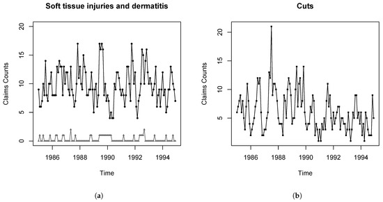
Figure 1. Monthly number of claims. (a) Soft tissue injuries claims (black dots) and dermatitis claims (gray triangles). (b) Cuts claims.

On the other hand, if one considers a bivariate series of soft tissue injuries claims and cuts claims, see Figure 1 (right panel), and tests the GOF for a Poisson BINAR model with a diagonal matrix $\mathbf{A}$ (which corresponds to univariate INAR models for the two series), the null hypothesis is rejected with p-value $0.0370$. A Poisson BINAR with a general matrix $\mathbf{A}$ is rejected as well (p-value $0.002$). This is in accordance with the findings of previous papers mentioned above. However, the hypothesis of BPAR is not rejected with p-value $0.277$. The MLEs in this model are $\widehat{\mathit{\alpha }}={(5.144,2.944)}^{\top }$, $\widehat{\varphi }=0.721$ and $\widehat{\mathbf{B}}$ is such that $\mathsf{vec}\left(\widehat{\mathbf{B}}\right)={(0.455,0.004,0.043,0.521)}^{\top }$. One could further scrutinize this data set by postulating an extended (nonstationary) BPAR model with a seasonal component. This might improve the models’ predictions compared to the fitted stationary model, but such a model lies outside the scope of this paper.

9. Concluding Remarks

We suggest consistent goodness-of-fit tests for bivariate INAR and bivariate Poisson autoregressive models, estimated by least squares and maximum likelihood, respectively, with well defined limit null distributions. Since these limit distributions are complicated we suggest parametric bootstrap resampling which engages distributional assumptions featuring in the null hypothesis in order to actually carry out the tests. Monte Carlo results show that this bootstrap version of the new tests is generally reasonably sized and has good power against certain popular alternative configurations. Our real-data applications are in the direction of further scrutiny and better understanding of the mechanisms generating the data at hand.

At this point, we wish to discuss potential extension of the tests to models of higher order or dimension, such as the multivariate INAR type processes studied by Franke and Rao (1995), Latour (1997), Pedeli and Karlis (2011), Pedeli and Karlis (2013c), and Pedeli and Karlis (2013a), and corresponding extensions of PAR type models considered by Liu (2012), Andreassen (2013), Lee et al. (2018), Ciu and Zhu (2018) and Ciu et al. (2020). In this connection, and while it is conceptually straightforward to extend the tests for INAR or PAR models of higher order, see also Section 6 of Hudecová et al. (2015), we wish to emphasize the fact that a certain order and/or dimension increase brings about serious challenges in estimation as well as on the actual implementation of the methods due to the potentially great number of new parameters introduced.

Finally, before we close, we wish to point out that while this paper deals solely with stationary time series models, certain real world phenomena, including time series of counts, often exhibit deterministic trends or seasonal patterns, and thus GOF tests for non-stationary models would be of great practical interest. However, despite the fact that univariate INAR and PAR models with deterministic components have been extensively studied in the literature, multivariate extensions of such nonstationary models are rather scarce; we refer to Santos et al. (2019) for some recent works.

Appendix A.1. Proof of Theorem 1

Proof. 

Denote as $\mathcal{A}\subset {[0,1]}^4$ such that if $\mathbf{a}\in \mathcal{A}$ then $\mathbf{A}$ has the largest eigenvalue smaller than 1. The test statistic $S_{n,\upsilon }$ is of the form

$$\begin{array}{cc}\hfill S_{n,\upsilon }& ={\int }_{{[0,1]}^2}{\left[\frac{1}{\sqrt{n}}\sum _{t=1}^n\left(u_1^{Y_{t,1}}{u}_2^{Y_{t,2}}-g_{\epsilon }(\mathbf{u},\widehat{\mathit{\theta }})W_t(\mathbf{u},\widehat{\mathbf{a}})\right)\right]}^2\upsilon \left(\mathbf{u}\right)\mathrm{d}\mathbf{u}\hfill \\ \hfill & ={\int }_{{[0,1]}^2}{\left[\frac{1}{\sqrt{n}}\sum _{t=2}^n\left(u_1^{Y_{t,1}}{u}_2^{Y_{t,2}}-g_{\epsilon }(\mathbf{u},\widehat{\mathit{\theta }})W_{t-1}(\mathbf{u},\widehat{\mathbf{a}})\right)\right]}^2\upsilon \left(\mathbf{u}\right)\mathrm{d}\mathbf{u}+o_P\left(1\right).\hfill \end{array}$$

Let $A_t=A_t(\mathit{\theta },\mathbf{a})=g_{\epsilon }(\mathbf{u},\mathit{\theta })W_t(\mathbf{u},\mathbf{a}).$ In the following, we omit for a moment the argument $\mathbf{u}$ in all the considered functions. Namely we consider $W_t=W_t\left(\mathbf{a}\right)$ as a function of the argument $\mathbf{a}$ alone, i.e., $\nabla W_t$ is a differential of $W_t$ with respect to $\mathbf{a}$, $\nabla W_t={\nabla }_{\mathbf{a}}{W}_t={(\partial W/\partial a_{11},\partial W/\partial a_{12},\partial W/\partial a_{21},\partial W/\partial a_{22})}^{\top }$. Likewise, $\nabla g_{\epsilon }={\nabla }_{\theta }{g}_{\epsilon }$ is a differential of $g_{\epsilon }$ with respect to $\mathit{\theta }$. Then a Taylor expansion gives:

$$A_t(\widehat{\mathit{\theta }},\widehat{\mathbf{a}})=A_t(\mathit{\theta },\mathbf{a})+{\left(\begin{array}{c}\widehat{\mathit{\theta }}-\mathit{\theta }\\ \widehat{\mathbf{a}}-\mathbf{a}\end{array}\right)}^{\top }\left(\begin{array}{c}{W}_t\left(\mathbf{a}\right)\nabla g_{\mathit{\epsilon }}\left(\mathit{\theta }\right)\\ g_{\mathit{\epsilon }}\left(\mathit{\theta }\right)\nabla W_t\left(\mathbf{a}\right)\end{array}\right)+R_t,$$

where

$$R_t=\frac{1}{2}{\left(\begin{array}{c}\widehat{\mathit{\theta }}-\mathit{\theta }\\ \widehat{\mathbf{a}}-\mathbf{a}\end{array}\right)}^{\top }\left(\begin{array}{cc}{W}_t\left({\mathbf{a}}^{\ast }\right)H_{g_{\epsilon }}\left({\mathit{\theta }}^{\ast }\right)& \nabla g_{\mathit{\epsilon }}\left({\mathit{\theta }}^{\ast }\right)\nabla W_t{\left({\mathbf{a}}^{\ast }\right)}^{\top }\\ \nabla W_t\left({\mathbf{a}}^{\ast }\right)\nabla g_{\mathit{\epsilon }}{\left({\mathit{\theta }}^{\ast }\right)}^{\top }& g_{\mathit{\epsilon }}\left({\mathit{\theta }}^{\ast }\right)H_{W_t}\left({\mathbf{a}}^{\ast }\right)\end{array}\right)\left(\begin{array}{c}\widehat{\mathit{\theta }}-\mathit{\theta }\\ \widehat{\mathbf{a}}-\mathbf{a}\end{array}\right),$$

with ${\mathbf{a}}^{\ast }=\widehat{\mathbf{a}}+c(\mathbf{a}-\widehat{\mathbf{a}})$ and ${\mathit{\theta }}^{\ast }=\widehat{\mathit{\theta }}+d(\mathit{\theta }-\widehat{\mathit{\theta }})$ for some $c,d\in (0,1)$ and where $H_{g_{\epsilon }}={\left({\partial }^2{g}_{\mathit{\epsilon }}/\left(\partial {\theta }_k\partial {\theta }_l\right)\right)}_{k,l}$ is the $k\times k$ matrix of second partial derivatives of $g_{\mathit{\epsilon }}$ with respect to $\mathit{\theta }$. Similarly, $H_{W_t}$ is the $4\times 4$ matrix of second partial derivatives of $W_t$ with respect to $\mathbf{a}$. For $\nabla W_t$ we have

$$\frac{\partial W_t}{\partial a_{ij}}=\frac{W_t}{w_{ij}^{Y_{t,j}}}{Y}_{t-1,j}{w}_{ij}^{Y_{t,j}-1}(u_i-1)=W_t\frac{Y_{t,j}}{w_{ij}}(u_i-1),$$

and clearly $\left|\partial W_t/\partial a_{ij}\right|\le Y_{tj}$ for all $\mathbf{u}\in {[0,1]}^2$ and $\mathbf{a}\in \mathcal{A}$. Furthermore,

$$\frac{{\partial }^2{W}_t}{\partial a_{ij}\partial a_{kl}}=\left\{\begin{array}{cc}{W}_t{\displaystyle \frac{Y_{t-1,j}{Y}_{t-1,l}}{w_{ij}{w}_{kl}}}(u_i-1)(u_k-1),\hfill & (i,j)\ne (k,l),\hfill \\ W_t{\displaystyle \frac{Y_{t-1,j}(Y_{t-1,j}-1)}{w_{ij}^2}}{(u_i-1)}^2\hfill & (i,j)=(k,l),\hfill \end{array}\right.$$

and thus, $\left|{\partial }^2{W}_t/(\partial a_{ij}\partial a_{kl})\right|\le Y_{t-1,j}{Y}_{t-1,l}$ for all $\mathbf{u}\in {[0,1]}^2$ and all $\mathbf{a}\in \mathcal{A}$.

Due to the finite second order moments of $\left\{{\mathbf{Y}}_t\right\}$ and Assumption (A.2) we have

$$\left|\frac{1}{\sqrt{n}}\sum _{t=2}^n{R}_t\right|\le K_1\sqrt{n}\parallel \widehat{\mathit{\theta }}{-\mathit{\theta }\parallel }^2+\sqrt{n}{\parallel \widehat{\mathbf{a}}-\mathbf{a}\parallel }^2{K}_2+K_3\sqrt{n}{(\widehat{\mathit{\theta }}-\mathit{\theta })}^{\top }{\mathbf{1}}_{k\times 4}(\widehat{\mathbf{a}}-\mathbf{a}),$$

where $K_i$ are constants and ${\mathbf{1}}_{k\times 4}$ is a matrix of 1’s of dimension $k\times 4$. Hence, it follows from the Cauchy–Schwartz inequality that ${\int }_{{[0,1]}^2}{\left|\frac{1}{\sqrt{n}}{\sum }_{t=2}^n{R}_t\right|}^2\upsilon \left(\mathbf{u}\right)\mathrm{d}\mathbf{u}\stackrel{𝖯}{\to }0,$ as $n\to \infty$, and thus the asymptotic distribution of $S_{n,\upsilon }$ is the same as the asymptotic distribution of

$${\int }_{{[0,1]}^2}{\left[J_{1n}(\mathit{\theta },\mathbf{a},\mathbf{u})+J_{2n}(\mathit{\theta },\mathbf{a},\mathbf{u})+J_{3n}(\mathit{\theta },\mathbf{a},\mathbf{u})\right]}^2\upsilon \left(\mathbf{u}\right)\mathrm{d}\mathbf{u},$$

where

$$\begin{array}{cc}\hfill J_{1n}(\mathit{\theta },\mathbf{a},\mathbf{u})& =\frac{1}{\sqrt{n}}\left(\sum _{t=2}^n{u}_1^{Y_{t,1}}{u}_2^{Y_{t,2}}-g_{\mathit{\epsilon }}(\mathbf{u},\mathit{\epsilon })W_{t-1}(\mathbf{u},\mathbf{a})\right),\hfill \\ \hfill J_{2n}(\mathit{\theta },\mathbf{a},\mathbf{u})& =-\sqrt{n}{(\widehat{\mathit{\theta }}-\mathit{\theta })}^{\top }\nabla g_{\mathit{\epsilon }}(\mathbf{u},\mathit{\theta })\frac{1}{n}\sum _{t=2}^n{W}_{t-1}(\mathbf{u},\mathbf{a}),\hfill \\ \hfill J_{3n}(\mathit{\theta },\mathbf{a},\mathbf{u})& =-g_{\mathit{\epsilon }}(\mathbf{u},\mathit{\theta })\sqrt{n}{(\widehat{\mathbf{a}}-\mathbf{a})}^{\top }\frac{1}{n}\sum _{t=2}^n{\nabla }_{\mathbf{a}}{W}_{t-1}(\mathbf{u},\mathbf{a}).\hfill \end{array}$$

Regarding the behavior of $J_{2n}$, notice that $|W_t\left(\mathbf{a}\right)|\le 1$ and thus, for a given $\mathbf{a}$ and as $n\to \infty$

$$\frac{1}{n}\sum _{t=2}^n{W}_{t-1}\left(\mathbf{a}\right)\stackrel{}{\to }\mathsf{E}{W}_1(\mathbf{u},\mathbf{a})=\mathsf{E}\prod _{i,j=1}^2{w}_{ij}^{Y_{1,j}}=g_{\mathbf{Y}}(w_{11}{w}_{21},w_{12}{w}_{22}),$$

uniformly in $\mathbf{u}\in {[0,1]}^2$ due to the uniform ergodicity theorem. Now define

$$J_{2n0}(\mathit{\theta },\mathbf{a},\mathbf{u})=-{\left[\frac{1}{\sqrt{n}}\sum _{t=q+1}^n{\mathbf{l}}_{t1}\right]}^{\top }{h}_2(\mathit{\theta },\mathbf{a},\mathbf{u}),$$

where $h_2(\mathit{\theta },\mathbf{a},\mathbf{u})={\nabla }_{\mathit{\theta }}{g}_{\mathit{\epsilon }}(\mathit{\theta },\mathbf{u})g_{\mathbf{Y}}(w_{11}{w}_{21},w_{12}{w}_{22}).$ Due to (A.2), it follows that ${\int }_{{[0,1]}^2}{[J_{2n}(\mathit{\theta },\mathbf{a},\mathbf{u})-J_{2n0}(\mathit{\theta },\mathbf{a},\mathbf{u})]}^2\upsilon \left(\mathbf{u}\right)\mathrm{d}\mathbf{u}=o_P\left(1\right)$ as $n\to \infty$. Similarly, in view of the form of $\nabla W_{t-1}\left(\mathbf{a}\right)$ given above and the finiteness of $\mathsf{E}{Y}_{1j}$, we get from the uniform ergodicity theorem that as $n\to \infty$

$$g_{\mathit{\epsilon }}(\mathit{\theta },\mathbf{a})\frac{1}{n}\sum _{t=2}^n\nabla W_{t-1}(\mathbf{u},\mathbf{a})\stackrel{𝖯}{\to }{g}_{\mathit{\epsilon }}(\mathbf{u},\mathit{\theta })\mathsf{E}\nabla W_1(\mathbf{u},\mathbf{a})=:h_3(\mathit{\theta },\mathbf{a},\mathbf{u})$$

uniformly in $\mathbf{u}\in {[0,1]}^2$. Define

$$J_{3n0}(\mathit{\theta },\mathbf{a},\mathbf{u})=-g_{\mathit{\epsilon }}(\mathit{\theta },\mathbf{u}){\left[\frac{1}{\sqrt{n}}\sum _{t=q+1}^n{\mathbf{l}}_{t2}\right]}^{\top }{h}_3(\mathit{\theta },\mathbf{a},\mathbf{u}).$$

As $|h_3(\mathit{\theta },\mathbf{a},\mathbf{u})|\le {max}_{j=1,2}\mathsf{E}{Y}_{1,j}$ then ${\int }_{{[0,1]}^2}{[J_{3n}(\mathit{\theta },\mathbf{a},\mathbf{u})-J_{3n0}(\mathit{\theta },\mathbf{a},\mathbf{u})]}^2\upsilon \left(\mathbf{u}\right)\mathrm{d}\mathbf{u}=o_P\left(1\right).$ Hence, it suffices to study the asymptotic behavior of ${\int }_{{[0,1]}^2}{Q}_n^2(\mathbf{u},\mathit{\theta },\mathbf{a})\upsilon \left(\mathbf{u}\right)\mathrm{d}\mathbf{u}$, where

$$Q_n(\mathbf{u},\mathit{\theta },\mathbf{a})=J_{1n0}(\mathit{\theta },\mathbf{a},\mathbf{u})+J_{2n0}(\mathit{\theta },\mathbf{a},\mathbf{u})+J_{3n0}(\mathit{\theta },\mathbf{a},\mathbf{u})$$

with $J_{1n0}(\mathit{\theta },\mathbf{a},\mathbf{u})=\frac{1}{\sqrt{n}}\left({\sum }_{t=q+1}^n{u}_1^{Y_{t,1}}{u}_2^{Y_{t,2}}-g_{\mathit{\epsilon }}(\mathbf{u},\mathit{\epsilon })W_{t-1}(\mathbf{u},\mathbf{a})\right)$. We will make use Theorem 22 from Ibragimov and Chasminskij (1981) and the subsequent remark in order to show that the integral ${\int }_{{[0,1]}^2}{Q}_n^2(\mathbf{u},\mathit{\theta },\mathbf{a})\upsilon \left(\mathbf{u}\right)d\mathbf{u}$ converges in distribution to ${\int }_{{[0,1]}^2}{Q}^2(\mathbf{u},\mathit{\theta },\mathbf{a})\upsilon \left(\mathbf{u}\right)d\mathbf{u}$, where Q is a Gaussian random field specified in the statement of the theorem. To this end, we need to verify that

• ${sup}_{n,\mathbf{u},\mathit{\theta },\mathbf{a}}\mathsf{E}{Q}_n^2(\mathbf{u},\mathit{\theta },\mathbf{a})<\infty .$
• There exist constants $\alpha >0$ and $H>0$ such that

  $$\underset{n,\mathit{\theta },\mathbf{a}}{sup}\mathsf{E}|Q_n(\mathbf{u},\mathit{\theta },\mathbf{a})-Q_n{(\mathbf{v},\mathit{\theta },\mathbf{a})|}^2\le H{\parallel \mathbf{u}-\mathbf{v}\parallel }^{\alpha }.$$
• The marginal distributions of $Q_n$ converge to the marginal distributions of Q uniformly in $\mathit{\theta }$ and $\mathbf{a}$.

First, notice that $Q_n$ is of a form $\frac{1}{\sqrt{n}}{\sum }_{t=q+1}^n{L}_t$, where $\left\{L_t\right\}$ is a martingale difference sequence $L_t=u_1^{Y_{t1}}{u}_2^{Y_{t2}}-g_{\epsilon }(\mathit{\theta },\mathbf{u})W_{t-1}(\mathbf{u},\mathbf{a})-{\mathbf{l}}_{t1}{(\mathit{\theta },\mathbf{a})}^{\top }{h}_2(\mathit{\theta },\mathbf{a},\mathbf{u})-{\mathbf{l}}_{t2}{(\mathit{\theta },\mathbf{a})}^{\top }{h}_3(\mathit{\theta },\mathbf{a},\mathbf{u})$. Thus $\mathsf{E}{Q}_n^2\le \frac{1}{n}{\sum }_{t=q+1}^n\mathsf{E}|L_t{|}^2\le 4(1+g_{\mathit{\epsilon }}^2+\parallel h_2{\parallel }^2\mathsf{E}\parallel l_{11}{\parallel }^2+\parallel h_3{\parallel }^2\mathsf{E}\parallel l_{12}{\parallel }^2).$ Since we assume finite variances of ${\mathbf{l}}_{t,j}$ and thus $\parallel h_j{\parallel }^2$ are bounded (due to finiteness of $\mathsf{E}{Y}_{t,j}$ and assumption A.2), condition I. directly follows. Condition III. follows from the central limit theorem for martingale difference sequences on $L_t$.

In order to prove condition II., we will show that $\mathsf{E}|J_{jn0}(\mathit{\theta },\mathbf{a},\mathbf{u})-J_{jn0}{(\mathit{\theta },\mathbf{a},\mathbf{v})|}^2\le D{\parallel \mathbf{u}-\mathbf{v}\parallel }^{\alpha }$ for $j=1,2,3$, for some $D>0$ and $\alpha >0$. In the following K is a generic constant. For $j=1$ we have

$$\begin{array}{cc}\hfill \mathsf{E}& |J_{1n0}(\mathit{\theta },\mathbf{a},\mathbf{u})-J_{1n0}{(\mathit{\theta },\mathbf{a},\mathbf{v})|}^2\hfill \\ \hfill & =\frac{1}{n}\mathsf{E}{\left\{\sum _{t=q+1}^n{u}_1^{Y_{t,1}}{u}_2^{Y_{t,2}}-v_1^{Y_{t,1}}{v}_2^{Y_{t,2}}-g_{\mathit{\epsilon }}\left(\mathbf{u}\right)W_{t-1}\left(\mathbf{u}\right)+g_{\mathit{\epsilon }}(\mathbf{v},\mathit{\theta })W_{t-1}(\mathbf{v},\mathbf{a})\right\}}^2\hfill \\ \hfill & \le K\{\mathsf{E}{[u_1^{Y_{t,1}}{u}_2^{Y_{t,2}}-v_1^{Y_{t,1}}{v}_2^{Y_{t,2}}]}^2+g_{\mathit{\epsilon }}{(\mathbf{u},\mathit{\theta })}^2\mathsf{E}{[W_1(\mathbf{u},\mathbf{a})-W_1(\mathbf{v},\mathbf{a})]}^2\hfill \\ \hfill & +{(g_{\mathit{\epsilon }}(\mathbf{u},\mathit{\theta })-g_{\mathit{\epsilon }}(\mathbf{v},\mathit{\theta }))}^2\mathsf{E}{\left|W_1(\mathbf{u},\mathbf{a})\right|}^2\}.\hfill \end{array}$$

By the mean value theorem applied on the function $f(x,y)=x^a{y}^b$ and due to the fact that $\mathsf{E}|Y_{t,j}|$ is finite, we get that $\mathsf{E}{[u_1^{Y_{t,1}}{u}_2^{Y_{t,2}}-v_1^{Y_{t,1}}{v}_2^{Y_{t,2}}]}^2\le K{\parallel \mathbf{u}-\mathbf{v}\parallel }^2.$ Next, $|g_{\mathit{\epsilon }}|\le 1$ and the partial derivatives $|\partial W_1/\partial u_j|$ are bounded by $|Y_{1,1}+Y_{1,2}|$, which has finite expectation. This implies that $g_{\mathit{\epsilon }}{(\mathbf{u},\mathit{\theta })}^2\mathsf{E}{[W_1(\mathbf{u},\mathbf{a})-W_1(\mathbf{v},\mathbf{a})]}^2\le K{\parallel \mathbf{u}-\mathbf{v}\parallel }^2.$ Finally, it follows from the definition of $g_{\mathit{\epsilon }}$ as a PGF that it is Lipschitz. Furthermore, $\mathsf{E}|W_1{(\mathbf{u},\mathbf{a})|}^2\le 1$, which implies ${(g_{\mathit{\epsilon }}(\mathbf{u},\theta )-g_{\mathit{\epsilon }}(\mathbf{v},\theta ))}^2\mathsf{E}|W_1{(\mathbf{u},\mathbf{a})|}^2\le K{\parallel \mathbf{u}-\mathbf{v}\parallel }^2.$ Together, we get $\mathsf{E}|J_{1n0}(\mathit{\theta },\mathbf{a},\mathbf{u})-J_{1n0}{(\mathit{\theta },\mathbf{a},\mathbf{v})|}^2\le K{\parallel \mathbf{u}-\mathbf{v}\parallel }^2.$ Similar arguments are used to show that the condition holds also for $j=3$. If we use the assumption that $l_t$ has finite variances, it remains to show that $\parallel h_j(\mathit{\theta },\mathbf{a},\mathbf{u})-h_j{(\mathit{\theta },\mathbf{a},\mathbf{v})\parallel }^2\le K{\parallel \mathbf{u}-\mathbf{v}\parallel }^{\alpha }.$ First, notice that the partial derivatives of $h_3$ with respect to $\mathbf{u}$ are continuous functions for $\mathbf{u}\in {[0,1]}^2$. Thus, they are bounded and we can apply the mean value theorem on the components of $h_3$, which implies that $\parallel h_3(\mathit{\theta },\mathbf{a},\mathbf{u})-h_3{(\mathit{\theta },\mathbf{a},\mathbf{v})\parallel }^2\le K{\parallel \mathbf{u}-\mathbf{v}\parallel }^2.$ Similarly, if the assumption (A.2) holds then the partial derivatives of $h_2$ are bounded and this implies that $\parallel h_2(\mathit{\theta },\mathbf{a},\mathbf{u})-h_2{(\mathit{\theta },\mathbf{a},\mathbf{v})\parallel }^2\le K{\parallel \mathbf{u}-\mathbf{v}\parallel }^2,$ which completes the proof of condition II., and thus the assertion of the theorem follows. □

Appendix A.2. Proof of Theorem 3

Proof. 

The proof proceeds along the same lines as the proof of Theorem 1. A Taylor expansion is used to show that

$$S_{n,\upsilon }={\int }_0^1{\int }_0^1{[J_0(\mathit{\theta },\mathbf{u})-J_1(\mathit{\theta },\mathbf{u})]}^2\upsilon \left(\mathbf{u}\right)\mathrm{d}\mathbf{u}+o_P\left(1\right),$$

where ${\mathbf{D}}_t\left(\mathbf{u}\right)$ are defined in the statement of the theorem,

$$\begin{array}{cc}\hfill J_0(\mathit{\theta },\mathbf{u})& =\frac{1}{\sqrt{n}}\sum _{t=2}^n\left[u_1^{Y_{t,1}}{u}_2^{Y_{t,2}}-f_{t-1}(\mathit{\theta },\mathbf{u})\right],\hfill \\ \hfill J_1(\mathit{\theta },\mathbf{u})& =n^{-1/2}\sum _{t=2}^n{f}_{t-1}(\mathit{\theta },\mathbf{u}){\mathbf{D}}_{t-1}{\left(\mathbf{u}\right)}^{\top }(\widehat{\mathit{\theta }}-\mathit{\theta }),\hfill \\ \hfill f_{t-1}(\mathit{\theta },\mathbf{u})& =c(\mathbf{u},\mathit{\theta })w_1{\left(\mathbf{u}\right)}^{Y_{t-1,1}}{w}_2{\left(\mathbf{u}\right)}^{Y_{t-1,2}}.\hfill \end{array}$$

The term $J_1(\mathit{\theta },\mathbf{u})$ can be replaced by $J_{10}(\mathit{\theta },\mathbf{u})=\left[\mathsf{E}{\mathbf{D}}_1{\left(\mathbf{u}\right)}^{\top }{f}_1(\mathit{\theta },\mathbf{u})\right]\left(n^{-1/2}{\sum }_{t=q}^n{\mathbf{l}}_t\right)$. Finally, the conditions I.–III. from Theorem 22 of Ibragimov and Chasminskij (1981) can be verified similarly as it is done for BINAR using the fact that the fourth moments of ${\mathbf{Y}}_t$ are finite and the parametric space $\mathsf{\Theta }$ is compact. □

References

- Ahmad, Ali, and Christian Francq. 2016. Poisson QMLE of count time series models. Journal of Time Series Analysis 37: 291–314. [Google Scholar] [CrossRef]
- Al-Osh, Mohamed A., and Abdulhamid A. Alzaid. 1987. First–order integer–valued autoregressive (INAR(1)) process. Journal of Time Series Analysis 8: 261–75. [Google Scholar] [CrossRef]
- Aleksandrov, Boris, and Christian H. Weiss. 2020. Testing the dispersion structure of count time series using Pearson residuals. AStA Advances in Statistical Analysis 104: 325–61. [Google Scholar] [CrossRef]
- Andreassen, Camilla Mondrup. 2013. Models and Inference for Correlated Count Data. Ph.D. thesis, Aarhus University, Aarhus, Denmark. [Google Scholar]
- Biswas, Atanu, and Peter Xue Kun Song. 2009. Discrete-valued ARMA processes. Statistics and Probability Letters 79: 1884–89. [Google Scholar] [CrossRef]
- Ciu, Yan, Qi Li, and Fukang Zhu. 2020. Flexible bivariate Poisson integer-valued GARCH model. Annals of the Institute of Statistical Mathematics 72: 1449–77. [Google Scholar]
- Ciu, Yan, and Fukang Zhu. 2018. A new bivariate integer-valued GARCH model allowing for negative cross-correlation. TEST 27: 428–52. [Google Scholar]
- Davis, Richard A., Scott H. Holan, Robert Lund, and Nalini Ravishanker. 2015. Handbook of Discrete-Valued Time Series. New York: Chapman and Hall/CRC. [Google Scholar]
- Davis, Richard A., and Heng Liu. 2016. Theory and inference for a class of nonlinear models with application to time series of counts. Statistica Sinica 26: 1673–707. [Google Scholar] [CrossRef][Green Version]
- Du, Jin-Guan, and Yuan Li. 1991. The integer-valued autoregressive (INAR(p)) model. Journal of Time Series Analysis 12: 129–42. [Google Scholar]
- Dunn, James E. 1967. Characterization of the bivariate negative binomial distribution. Journal of the Arkansas Academy of Science 21: 77–86. [Google Scholar]
- Esquível, Manuel L. 2008. Probability generating functions for discrete real–valued random variables. Theory of Probability and Its Applications 52: 40–57. [Google Scholar] [CrossRef]
- Ferland, René, Alain Latour, and Driss Oraichi. 2006. Integer-valued GARCH processes. Journal of Time Series Analysis 27: 923–42. [Google Scholar] [CrossRef]
- Fokianos, Konstantinos. 2012. Count time series. In Handbook of Statistics 30: Time Series—Methods and Applications. Edited by Tata Subba Rao, Suhasini Subba Rao and Calyampudi Radhakrishna Rao. Amsterdam: Elsevier, pp. 315–47. [Google Scholar]
- Fokianos, Konstantinos, and Michael H. Neumann. 2013. A goodness–of–fit tests for Poisson count processes. Electronic Journal of Statistics 7: 793–819. [Google Scholar] [CrossRef]
- Fokianos, Konstantinos, Andres Rahbek, and Dag Tjøstheim. 2009. Poisson autoregression. Journal of the American Statistical Association 104: 1430–39. [Google Scholar] [CrossRef]
- Fokianos, Konstantinos, and Dag Tjøstheim. 2012. Nonlinear Poisson autoregression. Annals of the Institute of Statistical Mathematics 64: 1205–25. [Google Scholar] [CrossRef]
- Franke, Jürgen, and T. Subba Rao. 1995. Multivariate First-Order Integer-Valued Autoregressions. Technical Report. Kaiserslautern: Universität Kaiserslautern. [Google Scholar]
- Freeland, R. Keith. 1998. Statistical Analysis of Discrete Time series with Application to the Analysis of Workers’ Compensation Claims Data. Ph.D. thesis, Management Science Division, Faculty of Commerce and Business Administration, University of British Columbia, Vancouver, BC, Canada. Available online: https://open.library.ubc.ca/cIRcle/collections/ubctheses (accessed on 25 February 2021).
- Freeland, R. Keith, and Brendan P. M. McCabe. 2004. Analysis of low count time series data by Poisson autoregression. Journal of Time Series Analysis 25: 701–22. [Google Scholar] [CrossRef]
- Giacomini, Raffaella, Dmitris Politis, and Halbert White. 2013. A warp-speed method for conducting Monte Carlo experiments involving bootstrap estimators. Econometric Theory 29: 567–89. [Google Scholar] [CrossRef]
- Heinen, Andréas, and Erick Rengifo. 2007. Multivariate autoregressive modeling of time series count data using copulas. Journal of Empirical Finance 14: 564–583. [Google Scholar] [CrossRef]
- Hudecová, Šárka, Marie Hušková, and Simos G. Meintanis. 2015. Tests for time series of counts based on the probability generating function. Statistics 49: 316–37. [Google Scholar] [CrossRef]
- Ibragimov, Il’dar Abdulovich, and Rafail Zalmonovich Chasminskij. 1981. Statistical Estimation, Asymptotic Theory. New York: Springer. [Google Scholar]
- Jiménez-Gamero, M. Dolores, Sangyeol Lee, and Simos G. Meintanis. 2020. Goodness-of-fit tests for parametric specifications of conditionally heteroscedastic models. TEST 29: 682–703. [Google Scholar] [CrossRef]
- Kim, Hanwool, and Sangyeol Lee. 2017. On first order integer-valued autoregressive process with Katz family innovations. Journal of Statistical Computation and Simulation 87: 546–62. [Google Scholar] [CrossRef]
- Kocherlakota, Subrahmaniam, and Kathleen Kocherlakota. 1992. Bivariate Discrete Distributions. New York: Marcel Dekker Inc. [Google Scholar]
- Lakshminarayana, J., S. N. Narahari Pandit, and K. Srinivasa Rao. 1999. On a bivariate Poisson distribution. Communications in Statistics—Theory and Methods 28: 267–76. [Google Scholar] [CrossRef]
- Latour, Alain. 1997. The multivariate GINAR(p) process. Advances in Applied Probability 29: 228–48. [Google Scholar] [CrossRef]
- Lee, Youngmi, Sangyeol Lee, and Dag Tjøstheim. 2018. Asymptotic normality and parameter change test for bivariate Poisson INGARCH models. TEST 27: 52–69. [Google Scholar] [CrossRef]
- Leucht, Anne, Jens-Peter Kreiss, and Michael H. Neumann. 2015. A model specification test for GARCH(1,1) processes. Scandinavian Journal of Statistics 42: 1167–93. [Google Scholar] [CrossRef]
- Liu, Heng. 2012. Some Models for Time Series of Counts. Ph.D. thesis, Columbia University, New York, NY, USA. [Google Scholar]
- Mamode Khan, Naushad Ali, Yuvraj Sunecher, Vandna Jowaheer, Miroslav M. Ristić, and Maleika Heenaye–Mamode Khan. 2019. Investigating GQL–based inferential approaches for non-stationary BINAR(1) model under different quantum of over-dispersion with application. Computational Statistics 34: 1275–313. [Google Scholar] [CrossRef]
- McKenzie, Eddie. 1985. Some simple models for discrete variate time series. Water Resources Bulletin 21: 645–50. [Google Scholar] [CrossRef]
- McKenzie, Eddie. 2003. Discrete variate time series. Stochastic Processes: Modelling and Simulation. In Handbook of Statistics. Amsterdam: Elsevier, vol. 21, pp. 573–606. [Google Scholar]
- Meintanis, Simos G., and Dimitris Karlis. 2014. Validation tests for the innovation distribution in INAR time series models. Computational Statistics 29: 1221–41. [Google Scholar] [CrossRef]
- Neumann, Michael H. 2011. Absolute regularity and ergodicity of Poisson count processes. Bernoulli 17: 1258–84. [Google Scholar] [CrossRef]
- Partrat, Christian. 1994. Compound model for two dependent kinds of claim. Insurance: Mathematics and Economics 15: 219–31. [Google Scholar] [CrossRef]
- Pedeli, Xanthi, and Dimitris Karlis. 2011. A bivariate INAR(1) process with application. Statistical Modelling 11: 325–49. [Google Scholar] [CrossRef]
- Pedeli, Xanthi, and Dimitris Karlis. 2013a. On composite likelihood estimation of a multivariate INAR(1) model. Journal of Time Series Analysis 34: 206–20. [Google Scholar] [CrossRef]
- Pedeli, Xanthi, and Dimitris Karlis. 2013b. On estimation of the bivariate Poisson INAR process. Communications in Statistics—Simulation and Computation 42: 514–33. [Google Scholar] [CrossRef]
- Pedeli, Xanthi, and Dimitris Karlis. 2013c. Some properties of multivariate INAR(1) processes. Computational Statistics & Data Analysis 67: 213–25. [Google Scholar]
- Popović, Predrag M., Aleksandar S. Nastić, and Miroslav M. Ristić. 2018. Residual analysis with bivariate INAR models. REVSTAT 16: 349–64. [Google Scholar]
- R Core Team. 2019. R: A Language and Environment for Statistical Computing. Vienna: R Foundation for Statistical Computing. [Google Scholar]
- Santos, Cláudia, Isabel Pereira, and Manuel G. Scotto. 2019. On the theory of periodic multivariate INAR processes. Statistical Papers. [Google Scholar] [CrossRef]
- Schweer, Sebastian. 2016. A goodness–of–fit test for integer valued autoregressive processes. Journal of Time Series Analysis 37: 77–98. [Google Scholar] [CrossRef]
- Schweer, Sebastian, and Christian H. Weiss. 2014. Compound Poisson INAR(1) processes: Stochastic properties and testing for overdispersion. Computational Statistics & Data Analysis 77: 267–84. [Google Scholar]
- Scotto, Manuel G., Christian H. Weiss, and Sónia Gouveia. 2015. Thinning-based models in the analysis of integer-valued time series: A review. Statistical Modelling 15: 590–618. [Google Scholar] [CrossRef]
- Shi, Peng, Xiaoping Feng, and Jean-Philippe Boucher. 2016. Multilevel modeling of insurance claims using copulas. The Annals of Applied Statistics 10: 834–36. [Google Scholar] [CrossRef]
- Steutel, Fred W., and Klaas van Harn. 1979. Discrete analogues of self-decomposability and stability. Annals of Probability 7: 893–99. [Google Scholar] [CrossRef]
- Vernic, Raluca. 1997. On the bivariate generalized poisson distribution. ASTIN Bulletin 27: 22–32. [Google Scholar] [CrossRef]
- Weiss, Christian H. 2018a. Discrete-Valued Time Series. Hoboken: John Wiley & Sons. [Google Scholar]
- Weiss, Christian H. 2018b. Goodness–of–fit testing of a count series’ marginal distribution. Metrika 81: 619–51. [Google Scholar] [CrossRef]
- Weiss, Christian H., Annika Homburg, and Pedro Puig. 2019. Testing for zero inflation and overdispersion in INAR(1) models. Statistical Papers 60: 473–98. [Google Scholar] [CrossRef]
- Weiss, Christian H., and Sebastian Schweer. 2015. Detecting overdispersion in INARCH(1) processes. Statistica Neerlandica 69: 281–97. [Google Scholar] [CrossRef]
- Zhu, Rong, and Harry Joe. 2006. Modelling count data time series with Markov processes based on binomial thinning. Journal of Time Series Analysis 27: 725–38. [Google Scholar] [CrossRef]
Publisher’s Note: MDPI stays neutral with regard to jurisdictional claims in published maps and institutional affiliations. |
© 2021 by the authors. Licensee MDPI, Basel, Switzerland. This article is an open access article distributed under the terms and conditions of the Creative Commons Attribution (CC BY) license (http://creativecommons.org/licenses/by/4.0/).