New York FED Staff Nowcasts and Reality: What Can We Learn about the Future, the Present, and the Past?  ^†

Abstract

We assess the forecasting performance of the nowcasting model developed at the New York FED. We show that the observation regarding a striking difference in the model’s predictive ability across business cycle phases made earlier in the literature also applies here. During expansions, the nowcasting model forecasts at best are at least as good as the historical mean model, whereas during the recessionary periods, there are very substantial gains corresponding in the reduction in MSFE of about 90% relative to the benchmark model. We show how the asymmetry in the relative forecasting performance can be verified by the use of such recursive measures of relative forecast accuracy as Cumulated Sum of Squared Forecast Error Difference (CSSFED) and Recursive Relative Mean Squared Forecast Error (based on Rearranged observations) (R²MSFE(+R)). Ignoring these asymmetries results in a biased judgement of the relative forecasting performance of the competing models over a sample as a whole, as well as during economic expansions, when the forecasting accuracy of a more sophisticated model relative to naive benchmark models tends to be overstated. Hence, care needs to be exercised when ranking several models by their forecasting performance without taking into consideration various states of the economy.

1. Introduction

The outbreak of the Great Financial Crisis about a decade ago significantly spurred the quest for reliable forecasting of economic conditions not only in the distant future, but also for reliable assessment of the current health of the economy. The forecasting academics and practitioners responded with developing of econometric models that specifically aim at forecasting GDP growth in the current or next quarter at most. This process of forecasting either the present or not that very distant past, or the future was naturally labelled as “nowcasting” (Banbura et al. 2011).

Among the recent contributions to the nowcasting literature, the project initiated and maintained at the Federal Reserve Bank of New York (FRBNY) is worth mentioning. The model described in the academic contribution of Bok et al. (2018) is promoted to the general public in a series of online blogs. The initial online announcement (Aarons et al. 2016) about the model and its regular nowcast releases made publicly available was made in 2016. The subsequent blog entry (Giannone et al. 2017) describes in the Q & A format—accessible to the general public—what nowcasting is and how the assessment of the current economic conditions is carried out by means of a pure data-driven approach. The model developers striving to achieve model transparency even went as far as putting the underlying code in the online code depository (Adams et al. 2018), such that anyone interested in nowcasting can go through the code and, if needed, adapt it for nowcasting of economic conditions in a country/region of their choice. More importantly, as initially announced, the nowcasts are regularly made public on the dedicated website in a forecast-as-you-go fashion since the inception of this project in 2016 (https://www.newyorkfed.org/research/policy/nowcast, accessed on 21 February 2021). In the most recent addition to the project, Adams et al. (2019) made the archive of nowcasts simulated backward for the period from 2002 to 2015 publicly available. As a result of this contribution, the sequence of nowcasts for every quarter since 2002 until the most recent one is available for analysis.

For our purposes, this most recent blog entry is important, as the sample for which nowcasts are available extends long enough in the past to include the Great Financial Crisis and it covers one complete business cycle period including both expansion and recession phases. In this study, we intend to verify the conclusions of Chauvet and Potter (2013) on asymmetric forecasting performance of the state-of-the-art macroeconometric models during expansionary and recessionary phases of the business cycle. This asymmetry displays itself in the fact that absolute forecasting errors during recessions tend to be larger than during expansions, i.e., the forecast accuracy, tend to decrease during economic downturns compared to economic upturns. Moreover, they find that during expansions, a simple univariate benchmark model that utilizes only its own past, delivers forecast accuracy that is comparable with that produced by very sophisticated models that draw information from various economic and financial indicators that are often available much earlier than official GDP releases. Since this aspect of the nowcasting performance of the model developed at the Federal Reserve Bank of New York is absent both in the online blog entries as well as in the published paper (Bok et al. 2018), it shapes the contribution of our study to the nowcasting literature. Namely, whether the conclusions of Chauvet and Potter (2013) reached for the other types of models can be generalized for the model in question.

Compared to the models utilized in Chauvet and Potter (2013), where for each quarter the accuracy of single one- and two-step ahead forecasts were evaluated, the output of the NY FRB Nowcasting model for each targeted quarter comprises a sequence of about 20 weekly nowcasts available for analysis. These weekly sequences of nowcasts provide us with additional information helping us to address the question of how far ahead in the future one can forecast using a weekly rather than a quarterly time scale definition.

Willingly or not, by making the historical record of model nowcasts publicly available, Adams et al. (2019) provide a benchmark that other forecasters may be tempted to use in order to compare nowcasting performance of their models, e.g., see Babii et al. (2019, p. 21) and Cimadomo et al. (2020). Interestingly enough, Bok et al. (2018) does not provide a formal comparison of the forecasting performance of their model with commonly used univariate benchmark models. This constitutes an additional motivation of our study, where we specifically evaluate the forecasting performance of the NY FED Nowcasting model relative to the univariate benchmark models for the full period and across business cycle phases. Our results can be informative for those studies that use NY FED Nowcasting model predictions of the US GDP growth as the benchmark. More generally, our research is related to such studies as Cai et al. (2019) and Alessi et al. (2014) where the actual forecasting experience at such policy-making institutions as ECB and FRBNY is scrutinized.

The rest of the paper is organized as follows. In Section 2, a review of the relevant literature is provided. The NY FED Nowcasting model and its output is detailed in Section 3. A description of benchmark models and forecast evaluation metrics used for model comparison is provided in Section 4 and Section 5, respectively. The accuracy of the nowcasting performance of the model against different releases of GDP data (advance, second, final, and latest) for the full sample as well as separately for the periods of the economic downturn (the Great Recession) and upturns is reported in Section 6. The final section concludes.

2. Literature Review

Instabilities in forecasting performance of macroeconometric models have been long acknowledged in the literature. For example, Rossi (2013) in a comprehensive review of the relevant literature points out at several stylized facts. First, the predictive strength of the variables substantially varies over time such that excellent predictive performance in the past does not warrant similar forecasting excellence in the near future, let alone the distant one. Second, model empirical validation, based on their performance in sample, often serves as a poor approximation of their forecasting ability out of sample.

While there are many potential reasons of unstable predictive ability of macroeconometric models, one explanation that seems obvious is the presence of the business cycles that at some more or less regular intervals shake up individual countries, whole regions, or even spread all over the globe. Naturally, the economic dynamics is completely different during recessions than expansions; hence, it is natural to expect that the forecasting performance varies with the state of the business cycle.

Rossi (2013) only briefly mentions business cycles as a possible explanation of forecasting instability, but a more thorough investigation of this topic is provided in Chauvet and Potter (2013). Chauvet and Potter (2013) specifically evaluated the predictive ability of several most widely used macroeconometric models using US GDP growth as an example. The list of these models includes the structural DSGE model, reduced-form VARs estimated using either Bayesian or frequentist approaches, the dynamic factor model with Markov–Switching mechanism, and the cumulative depth of recession model. The conclusions reached in Chauvet and Potter (2013) are surprisingly uniform across these very diverse models. First, the forecasting accuracy of the models worsened in recessions, i.e., on average, forecast errors tended to be larger in economic downturns than during upturns. Second, during expansions, the forecasting performance of highly sophisticated models was matched by that of a simple univariate autoregressive benchmark model.

Siliverstovs (2020a) extends the analysis of Chauvet and Potter (2013) to a different class of models, namely, models that combine data observed at the heterogeneous frequencies: quarterly GDP growth and several monthly economic and financial indicators, such as industry production, sentiment indices, labor-market and housing statistics, stock market index, and interest rates that are commonly used for assessing current economic conditions in the US. In particular, Siliverstovs (2020a) re-examines the forecasting performance of a multiple-indicator U-MIDAS-type model suggested in Carriero et al. (2015). The model generalises the Unrestricted MIDAS model suggested in Foroni et al. (2015) in several directions by allowing more than one skip-sampled explanatory variable, optional inclusion of stochastic volatility, and Bayesian estimation of model parameters. The adopted mixed-frequency setup allows to monitor changes in the forecast accuracy as more information can be incorporated in the forecasting model from one month to another, in contrast to Chauvet and Potter (2013), where forecasts were made once per quarter.

Siliverstovs (2020a) shows that, at first glance, the impressive reduction in the RMSFE over the benchmark AR(2) model up to 22% reported in Carriero et al. (2015), when evaluated over the whole forecast sample from 1985Q1 until 2011Q3, is mainly driven by a few observations during recessions, with the most prominent contribution being traced to those observations during the Great Recession. Evaluation of the model’s forecasting performance during NBER recessions and expansions indicates that, during expansions, the performance of this model is closely matched by that of the benchmark model, conforming with the conclusion of Chauvet and Potter (2013). At the same time, it is worthwhile pointing out that during recessions the improvement over the benchmark model is very dramatic—almost up to 60% in terms of the RMSFE. All in all, it seems that ignoring the asymmetry in the forecasting performance of a more sophisticated model over a benchmark model results in a biased assessment of the model forecasting performance. The predictive ability of the former model tends to be overstated during expansions that last longer than recessions, but at the same time, it is severely understated during rather rare recessions, when prevailing economic distress makes demands for accurate forecasts more acute.

The findings of Chauvet and Potter (2013) and Siliverstovs (2020a), reported for a single time series (US GDP growth), were extended in Siliverstovs and Wochner (2021) for each time series in the Stock–Watson dataset comprising more than 200 US macroeconomic variables. The aim of this exercise was to replicate the study of Stock and Watson (2002) on a more recent data vintage but evaluate the forecasting performance of the diffusion-index model separately for the NBER expansions and recessions in a similar way as done in Chauvet and Potter (2013).

Siliverstovs and Wochner (2021) confirm that there are systematic differences in forecasting accuracy across the business cycle phases both in absolute and relative terms with respect to the benchmark models. During expansions, both diffusion-index models and benchmark models generally display similar forecasting performance. However, the more sophisticated model tends to yield substantial forecasting gains around turning points relative to the benchmark models. Quite often, such forecasting gains of the complicated model outweigh its relative losses during economic upturns, such that when the models are judged on the basis of their average forecasting performance over the whole forecast evaluation period, the actual performance of more sophisticated models is overstated, making it appear better in normal times than it really is. The opposite side of the coin is that its performance during recessions tends to be understated.

3. Nowcasting Framework

3.1. Model

The NY FED Nowcasting model is similar to the one introduced in Giannone et al. (2008). This dynamic factor model conveniently accommodates features of the data that a forecaster faces when making forecasts in real time. These data features include mixed-frequency data, i.e., GDP data available at the quarterly frequency and auxiliary economic and financial data that often are released at the monthly or even higher frequency. A data set of the auxiliary indicators can be unbalanced both at the beginning of the sample as well as at the end of the sample. Missing data at the beginning of the sample arise most often due to the fact that some time series began earlier or later than others. Missing data at the current edge are due to differences in the release timing of different indicators during a month and because of different publication lags of these indicators. For example, indicators released at the end of the current month can have the latest available observation either for the current month, the previous month, or even for a month further back in the past. In fact, the nowcasting framework developed in Giannone et al. (2008) proved very robust to such challenges posed by the above characteristics of economic data. In case of nowcasting, the GDP growth in Switzerland, once coded at the end of 2009, it ran reliably without a single breakdown during weekly nowcasting exercises at the KOF Swiss Economic Institute (ETH Zurich). The model is described in Siliverstovs and Kholodilin (2012) and the track of its nowcasting performance in real time squared is documented in Siliverstovs (2012) and Siliverstovs (2017).

3.2. Timing

Since the nowcasting project of the NY FED goes on, we have to truncate the information flow to reflect the data availability at the time of writing. More specifically, we evaluate the accuracy of nowcasts using the period from 2002Q1 until 2020Q2. For every quarter in this sample, we collected sequence of 21 nowcasts released at a weekly frequency. For several quarters, the number of weekly nowcasts exceeds 21. We chose to concentrate on these 21 weekly forecasts because in this case we obtain an equal number of forecasts for each quarter. This makes our measures of forecasting accuracy which we compute at each forecast origin comparable. The limiting factor was that the sequence of nowcasts for quarter 2018Q1 started one week later than it was usually made for other quarters and it comprises exactly 21 weekly forecasts. The first nowcast in this sequence is released 20 weeks ahead of the week when advance GDP estimate for the targeted quarter is published. The second nowcast precedes the advance GDP release by 19 weeks, and so on. The release of the last nowcast for the targeted quarter coincides with the timing of the release of the advance GDP estimate for this quarter which typically takes place at the end of the first month following the end of the quarter in question. Given such weekly releases, we label nowcasts by their forecast origin measuring the distance by the number of weeks preceding the week when the final nowcast for each quarter was released.

For example, the sequence of nowcasts for quarter 2009Q3—the first quarter after the end of the Great Recession—is shown in Figure 1 together with the second estimate of GDP growth in this quarter. There are several GDP releases—advance, second, and final that are sequentially released at the end of the first, second and third months of the following quarter—they can be compared with the nowcasts. In addition, one can compare nowcasts with GDP growth estimates from the vintage (released on 30 September 2020) that was available to us at the time of writing this manuscript. In the main text, we describe the results with respect to the second estimates of GDP growth. In the Appendix A, we verify robustness of our results by evaluating forecast accuracy for other versions of GDP releases: advance, final and latest, see

Table A1. Forecast accuracy, 2002Q1–2019Q4/2002Q1–2020Q2.

	Advance GDP Release
	2002Q1–2019Q4									2002Q1–2020Q2
	Full Sample			Boom			Bust			Full Sample			Bust
Weeks	DFM	HMM	ARM	DFM	HMM	ARM	DFM	HMM	ARM	DFM	HMM	ARM	DFM	HMM	ARM
20	4.69	4.05	3.95	3.32	1.85	2.11	17.36	24.51	21.05	20.59	21.95	21.66	145.31	167.13	162.86
19	4.28	4.05	3.95	3.01	1.85	2.11	16.04	24.51	21.05	19.47	21.95	21.66	138.31	167.13	162.86
18	4.22	4.05	3.95	2.97	1.85	2.11	15.75	24.51	21.05	19.51	21.95	21.66	138.93	167.13	162.86
17	3.84	4.05	3.95	3.04	1.85	2.11	11.32	24.51	21.05	18.53	21.95	21.66	130.37	167.13	162.86
16	3.72	4.05	3.95	2.94	1.85	2.11	11.00	24.51	21.05	18.36	21.95	21.66	129.69	167.13	162.86
15	3.26	4.05	3.95	2.86	1.85	2.11	6.97	24.51	21.05	12.20	21.95	21.66	79.68	167.13	162.86
14	3.28	4.05	4.01	2.93	1.85	2.17	6.56	24.51	21.05	12.28	21.95	21.71	79.81	167.13	162.86
13	3.33	4.03	3.46	2.99	1.85	2.14	6.51	24.25	15.74	11.30	21.89	19.41	71.27	166.63	144.12
12	3.20	4.03	3.52	2.89	1.85	2.20	6.06	24.25	15.74	3.72	21.89	19.46	9.65	166.63	144.12
11	2.98	4.03	3.52	2.73	1.85	2.20	5.28	24.25	15.74	3.46	21.89	19.46	8.73	166.63	144.12
10	2.71	4.03	3.52	2.50	1.85	2.20	4.66	24.25	15.74	3.34	21.89	19.46	9.41	166.63	144.12
9	2.52	4.03	3.52	2.37	1.85	2.20	3.93	24.25	15.74	3.20	21.89	19.46	9.15	166.63	144.12
8	2.45	4.03	3.52	2.32	1.85	2.20	3.62	24.25	15.74	3.70	21.89	19.46	13.62	166.63	144.12
7	2.25	4.03	3.52	2.11	1.85	2.20	3.60	24.25	15.74	3.40	21.89	19.46	12.77	166.63	144.12
6	2.12	4.03	3.52	1.97	1.85	2.20	3.47	24.25	15.74	5.19	21.89	19.46	28.46	166.63	144.12
5	2.04	4.03	3.52	1.91	1.85	2.20	3.22	24.25	15.74	6.26	21.89	19.46	37.67	166.63	144.12
4	1.72	4.03	3.52	1.77	1.85	2.20	1.34	24.25	15.74	6.49	21.89	19.46	40.63	166.63	144.12
3	1.70	4.03	3.52	1.72	1.85	2.20	1.54	24.25	15.74	6.36	21.89	19.46	39.93	166.63	144.12
2	1.66	4.03	3.52	1.71	1.85	2.20	1.26	24.25	15.74	6.55	21.89	19.46	41.54	166.63	144.12
1	1.64	4.03	3.52	1.67	1.85	2.20	1.34	24.25	15.74	6.54	21.89	19.46	41.76	166.63	144.12
0	1.65	4.03	3.52	1.68	1.85	2.20	1.35	24.25	15.74	6.83	21.89	19.46	44.02	166.63	144.12

Note: The table entries are the MSFEs computed for the advance GDP release. The MSFEs are computed for each model in each forecast round measured in terms of the approximate number of weeks preceding the release of the advance GDP estimate. The left panel reports the results for the pre-COVID sample, whereas the right panel refers to the full sample available. The defined expansionary period (BOOM) covers 2002Q1–2007Q3 and 2009Q3–2019Q4, and, since they are identical for both the left and right panels, the corresponding results are reported only in the left panel.

,

Table A2. Relative forecast accuracy, 2002Q1–2019Q4/2002Q1–2020Q2.

	Advance GDP Release
	2002Q1–2019Q4						2002Q1–2020Q2
	Full Sample		Boom		Bust		Full Sample		Bust
Weeks (Columns)	DFM/HMM (1)	ARM/HMM (2)	DFM/HMM (3)	ARM/HMM (4)	DFM/HMM (5)	ARM/HMM (6)	DFM/HMM (7)	ARM/HMM (8)	DFM/HMM (9)	ARM/HMM (10)
20	0.157	−0.026	0.796	0.139	−0.292	−0.141	−0.062	−0.013	−0.131	−0.026
19	0.056	−0.026	0.629	0.139	−0.346	−0.141	−0.113	−0.013	−0.172	−0.026
18	0.041	−0.026	0.608	0.139	−0.357	−0.141	−0.111	−0.013	−0.169	−0.026
17	−0.052	−0.026	0.643	0.139	−0.538	−0.141	−0.156	−0.013	−0.220	−0.026
16	−0.081	−0.026	0.590	0.139	−0.551	−0.141	−0.164	−0.013	−0.224	−0.026
15	−0.196	−0.026	0.546	0.139	−0.716	−0.141	−0.444	−0.013	−0.523	−0.026
14	−0.191	−0.012	0.580	0.172	−0.732	−0.141	−0.441	−0.011	−0.522	−0.026
13	−0.172	−0.140	0.619	0.158	−0.732	−0.351	−0.484	−0.113	−0.572	−0.135
12	−0.205	−0.127	0.564	0.189	−0.750	−0.351	−0.830	−0.111	−0.942	−0.135
11	−0.260	−0.127	0.478	0.189	−0.782	−0.351	−0.842	−0.111	−0.948	−0.135
10	−0.327	−0.127	0.352	0.189	−0.808	−0.351	−0.847	−0.111	−0.944	−0.135
9	−0.373	−0.127	0.282	0.189	−0.838	−0.351	−0.854	−0.111	−0.945	−0.135
8	−0.392	−0.127	0.256	0.189	−0.851	−0.351	−0.831	−0.111	−0.918	−0.135
7	−0.441	−0.127	0.139	0.189	−0.851	−0.351	−0.845	−0.111	−0.923	−0.135
6	−0.475	−0.127	0.064	0.189	−0.857	−0.351	−0.763	−0.111	−0.829	−0.135
5	−0.495	−0.127	0.031	0.189	−0.867	−0.351	−0.714	−0.111	−0.774	−0.135
4	−0.572	−0.127	−0.046	0.189	−0.945	−0.351	−0.703	−0.111	−0.756	−0.135
3	−0.578	−0.127	−0.072	0.189	−0.936	−0.351	−0.709	−0.111	−0.760	−0.135
2	−0.587	−0.127	−0.078	0.189	−0.948	−0.351	−0.701	−0.111	−0.751	−0.135
1	−0.594	−0.127	−0.098	0.189	−0.945	−0.351	−0.701	−0.111	−0.749	−0.135
0	−0.591	−0.127	−0.092	0.189	−0.944	−0.351	−0.688	−0.111	−0.736	−0.135

Note: Table entries are rMSFE of the DFM or ARM with respect to the benchmark HMM computed for the advance GDP release. The rMSFEs are computed using the corresponding entries in Table A1. For additional information, please see the notes in that table.

,

Table A3. Forecast accuracy, 2002Q1–2019Q4/2002Q1–2020Q2.

	Final GDP ReleasE
	2002Q1–2019Q4									2002Q1–2020Q2
	Full Sample			Boom			Bust			Full Sample			Bust
Weeks	DFM	HMM	ARM	DFM	HMM	ARM	DFM	HMM	ARM	DFM	HMM	ARM	DFM	HMM	ARM
20	5.95	5.02	4.94	4.20	2.51	2.78	22.18	28.31	24.93	20.49	21.50	21.23	138.11	158.63	154.47
19	5.69	5.02	4.94	4.09	2.51	2.78	20.61	28.31	24.93	19.55	21.50	21.23	131.26	158.63	154.47
18	5.64	5.02	4.94	4.07	2.51	2.78	20.24	28.31	24.93	19.60	21.50	21.23	131.76	158.63	154.47
17	5.33	5.02	4.94	4.20	2.51	2.78	15.81	28.31	24.93	18.70	21.50	21.23	123.41	158.63	154.47
16	5.20	5.02	4.94	4.10	2.51	2.78	15.41	28.31	24.93	18.52	21.50	21.23	122.69	158.63	154.47
15	4.58	5.02	4.94	3.97	2.51	2.78	10.22	28.31	24.93	12.52	21.50	21.23	74.31	158.63	154.47
14	4.63	5.02	4.99	4.06	2.51	2.85	9.87	28.31	24.93	12.63	21.50	21.29	74.46	158.63	154.47
13	4.62	5.00	4.60	4.05	2.52	2.95	9.91	28.06	19.91	11.65	21.45	19.20	66.50	158.15	136.59
12	4.39	5.00	4.65	3.87	2.52	3.01	9.18	28.06	19.91	4.87	21.45	19.26	12.08	158.15	136.59
11	4.04	5.00	4.65	3.69	2.52	3.01	7.24	28.06	19.91	4.48	21.45	19.26	10.17	158.15	136.59
10	3.61	5.00	4.65	3.19	2.52	3.01	7.57	28.06	19.91	4.19	21.45	19.26	11.43	158.15	136.59
9	3.39	5.00	4.65	3.07	2.52	3.01	6.34	28.06	19.91	4.22	21.45	19.26	12.50	158.15	136.59
8	3.30	5.00	4.65	3.02	2.52	3.01	5.91	28.06	19.91	4.29	21.45	19.26	13.46	158.15	136.59
7	2.99	5.00	4.65	2.79	2.52	3.01	4.89	28.06	19.91	3.90	21.45	19.26	11.96	158.15	136.59
6	3.04	5.00	4.65	2.87	2.52	3.01	4.54	28.06	19.91	5.58	21.45	19.26	25.16	158.15	136.59
5	2.88	5.00	4.65	2.74	2.52	3.01	4.13	28.06	19.91	6.46	21.45	19.26	33.34	158.15	136.59
4	2.67	5.00	4.65	2.64	2.52	3.01	2.88	28.06	19.91	6.74	21.45	19.26	36.36	158.15	136.59
3	2.65	5.00	4.65	2.61	2.52	3.01	2.97	28.06	19.91	6.63	21.45	19.26	35.64	158.15	136.59
2	2.60	5.00	4.65	2.66	2.52	3.01	2.04	28.06	19.91	6.76	21.45	19.26	36.33	158.15	136.59
1	2.57	5.00	4.65	2.63	2.52	3.01	2.04	28.06	19.91	6.75	21.45	19.26	36.47	158.15	136.59
0	2.57	5.00	4.65	2.63	2.52	3.01	1.97	28.06	19.91	6.99	21.45	19.26	38.49	158.15	136.59

Note: The table entries are the MSFEs computed for the final GDP release. The MSFEs are computed for each model in each forecast round measured in terms of the approximate number of weeks preceding the release of the advance GDP estimate. The left panel reports the results for the pre-COVID sample, whereas the right panel refers to the full sample available. The defined expansionary period (BOOM) covers 2002Q1–2007Q3 and 2009Q3–2019Q4, and, since they are identical for both the left and right panels, the corresponding results are reported only in the left panel.

,

Table A4. Relative forecast accuracy, 2002Q1–2019Q4/2002Q1–2020Q2.

	Final GDP Release
	2002Q1–2019Q4						2002Q1–2020Q2
	Full Sample		Boom		Bust		Full Sample		Bust
Weeks (Columns)	DFM/HMM (1)	ARM/HMM (2)	DFM/HMM (3)	ARM/HMM (4)	DFM/HMM (5)	ARM/HMM (6)	DFM/HMM (7)	ARM/HMM (8)	DFM/HMM (9)	ARM/HMM (10)
20	0.185	−0.017	0.672	0.107	−0.216	−0.119	−0.047	−0.013	−0.129	−0.026
19	0.134	−0.017	0.626	0.107	−0.272	−0.119	−0.091	−0.013	−0.173	−0.026
18	0.123	−0.017	0.619	0.107	−0.285	−0.119	−0.088	−0.013	−0.169	−0.026
17	0.062	−0.017	0.672	0.107	−0.442	−0.119	−0.130	−0.013	−0.222	−0.026
16	0.035	−0.017	0.630	0.107	−0.455	−0.119	−0.139	−0.013	−0.227	−0.026
15	−0.089	−0.017	0.579	0.107	−0.639	−0.119	−0.417	−0.013	−0.532	−0.026
14	−0.079	−0.006	0.616	0.132	−0.651	−0.119	−0.413	−0.010	−0.531	−0.026
13	−0.075	−0.080	0.610	0.173	−0.647	−0.290	−0.457	−0.104	−0.579	−0.136
12	−0.123	−0.070	0.537	0.195	−0.673	−0.290	−0.773	−0.102	−0.924	−0.136
11	−0.193	−0.070	0.465	0.195	−0.742	−0.290	−0.791	−0.102	−0.936	−0.136
10	−0.278	−0.070	0.265	0.195	−0.730	−0.290	−0.805	−0.102	−0.928	−0.136
9	−0.323	−0.070	0.218	0.195	−0.774	−0.290	−0.803	−0.102	−0.921	−0.136
8	−0.341	−0.070	0.198	0.195	−0.789	−0.290	−0.800	−0.102	−0.915	−0.136
7	−0.402	−0.070	0.107	0.195	−0.826	−0.290	−0.818	−0.102	−0.924	−0.136
6	−0.393	−0.070	0.140	0.195	−0.838	−0.290	−0.740	−0.102	−0.841	−0.136
5	−0.425	−0.070	0.088	0.195	−0.853	−0.290	−0.699	−0.102	−0.789	−0.136
4	−0.467	−0.070	0.049	0.195	−0.897	−0.290	−0.686	−0.102	−0.770	−0.136
3	−0.471	−0.070	0.037	0.195	−0.894	−0.290	−0.691	−0.102	−0.775	−0.136
2	−0.480	−0.070	0.056	0.195	−0.927	−0.290	−0.685	−0.102	−0.770	−0.136
1	−0.486	−0.070	0.043	0.195	−0.927	−0.290	−0.686	−0.102	−0.769	−0.136
0	−0.487	−0.070	0.044	0.195	−0.930	−0.290	−0.674	−0.102	−0.757	−0.136

Note: Table entries are rMSFE of the DFM or ARM with respect to the benchmark HMM computed for the final GDP release. The rMSFEs are computed using the corresponding entries in Table A3. For additional information, please see the notes in that table.

,

Table A5. Forecast accuracy, 2002Q1–2019Q4/2002Q1–2020Q2.

	Latest GDP Release
	2002Q1–2019Q4									2002Q1–2020Q2
	Full Sample			Boom			Bust			Full Sample			Bust
Weeks	DFM	HMM	ARM	DFM	HMM	ARM	DFM	HMM	ARM	DFM	HMM	ARM	DFM	HMM	ARM
20	6.38	5.73	5.44	3.65	2.41	2.45	31.75	36.55	33.16	20.90	22.18	21.71	145.50	164.98	160.81
19	6.11	5.73	5.44	3.57	2.41	2.45	29.71	36.55	33.16	19.95	22.18	21.71	138.29	164.98	160.81
18	6.03	5.73	5.44	3.52	2.41	2.45	29.28	36.55	33.16	19.97	22.18	21.71	138.75	164.98	160.81
17	5.78	5.73	5.44	3.71	2.41	2.45	25.05	36.55	33.16	19.14	22.18	21.71	130.55	164.98	160.81
16	5.60	5.73	5.44	3.54	2.41	2.45	24.72	36.55	33.16	18.90	22.18	21.71	129.88	164.98	160.81
15	5.00	5.73	5.44	3.57	2.41	2.45	18.22	36.55	33.16	12.93	22.18	21.71	80.48	164.98	160.81
14	5.02	5.73	5.47	3.64	2.41	2.49	17.91	36.55	33.16	13.00	22.18	21.74	80.65	164.98	160.81
13	4.99	5.70	4.97	3.53	2.40	2.52	18.54	36.28	27.74	12.00	22.12	19.56	73.16	164.48	142.61
12	4.74	5.70	5.01	3.38	2.40	2.56	17.35	36.28	27.74	5.21	22.12	19.60	18.38	164.48	142.61
11	4.37	5.70	5.01	3.30	2.40	2.56	14.31	36.28	27.74	4.80	22.12	19.60	15.62	164.48	142.61
10	4.04	5.70	5.01	2.84	2.40	2.56	15.19	36.28	27.74	4.60	22.12	19.60	17.30	164.48	142.61
9	3.80	5.70	5.01	2.77	2.40	2.56	13.39	36.28	27.74	4.61	22.12	19.60	17.92	164.48	142.61
8	3.71	5.70	5.01	2.75	2.40	2.56	12.62	36.28	27.74	4.68	22.12	19.60	18.62	164.48	142.61
7	3.53	5.70	5.01	2.79	2.40	2.56	10.44	36.28	27.74	4.42	22.12	19.60	16.22	164.48	142.61
6	3.26	5.70	5.01	2.64	2.40	2.56	9.04	36.28	27.74	5.80	22.12	19.60	28.61	164.48	142.61
5	3.12	5.70	5.01	2.52	2.40	2.56	8.62	36.28	27.74	6.69	22.12	19.60	36.78	164.48	142.61
4	3.00	5.70	5.01	2.48	2.40	2.56	7.88	36.28	27.74	7.07	22.12	19.60	40.20	164.48	142.61
3	2.98	5.70	5.01	2.44	2.40	2.56	7.97	36.28	27.74	6.94	22.12	19.60	39.47	164.48	142.61
2	2.88	5.70	5.01	2.51	2.40	2.56	6.26	36.28	27.74	7.02	22.12	19.60	39.57	164.48	142.61
1	2.89	5.70	5.01	2.54	2.40	2.56	6.08	36.28	27.74	7.05	22.12	19.60	39.57	164.48	142.61
0	2.90	5.70	5.01	2.57	2.40	2.56	5.95	36.28	27.74	7.31	22.12	19.60	41.55	164.48	142.61

Note: The table entries are the MSFEs computed for the latest GDP release. The MSFEs are computed for each model in each forecast round measured in terms of the approximate number of weeks preceding the release of the advance GDP estimate. The left panel reports the results for the pre-COVID sample, whereas the right panel refers to the full sample available. The defined expansionary period (BOOM) covers 2002Q1–2007Q3 and 2009Q3–2019Q4, and, since they are identical for both the left and right panels, the corresponding results are reported only in the left panel.

and

Table A6. Relative forecast accuracy, 2002Q1–2019Q4/2002Q1–2020Q2.

	Latest GDP Release
	2002Q1–2019Q4						2002Q1–2020Q2
	Full Sample		Boom		Bust		Full Sample		Bust
Weeks (Columns)	DFM/HMM (1)	ARM/HMM (2)	DFM/HMM (3)	ARM/HMM (4)	DFM/HMM (5)	ARM/HMM (6)	DFM/HMM (7)	ARM/HMM (8)	DFM/HMM (9)	ARM/HMM (10)
20	0.114	−0.051	0.515	0.017	−0.131	−0.093	−0.058	−0.021	−0.118	−0.025
19	0.066	−0.051	0.481	0.017	−0.187	−0.093	−0.101	−0.021	−0.162	−0.025
18	0.052	−0.051	0.463	0.017	−0.199	−0.093	−0.100	−0.021	−0.159	−0.025
17	0.010	−0.051	0.541	0.017	−0.315	−0.093	−0.137	−0.021	−0.209	−0.025
16	−0.023	−0.051	0.468	0.017	−0.324	−0.093	−0.148	−0.021	−0.213	−0.025
15	−0.127	−0.051	0.484	0.017	−0.502	−0.093	−0.417	−0.021	−0.512	−0.025
14	−0.123	−0.044	0.511	0.034	−0.510	−0.093	−0.414	−0.020	−0.511	−0.025
13	−0.124	−0.128	0.471	0.047	−0.489	−0.236	−0.457	−0.116	−0.555	−0.133
12	−0.168	−0.121	0.408	0.066	−0.522	−0.236	−0.765	−0.114	−0.888	−0.133
11	−0.233	−0.121	0.374	0.066	−0.606	−0.236	−0.783	−0.114	−0.905	−0.133
10	−0.291	−0.121	0.180	0.066	−0.581	−0.236	−0.792	−0.114	−0.895	−0.133
9	−0.333	−0.121	0.151	0.066	−0.631	−0.236	−0.792	−0.114	−0.891	−0.133
8	−0.350	−0.121	0.142	0.066	−0.652	−0.236	−0.789	−0.114	−0.887	−0.133
7	−0.380	−0.121	0.160	0.066	−0.712	−0.236	−0.800	−0.114	−0.901	−0.133
6	−0.428	−0.121	0.097	0.066	−0.751	−0.236	−0.738	−0.114	−0.826	−0.133
5	−0.453	−0.121	0.049	0.066	−0.762	−0.236	−0.698	−0.114	−0.776	−0.133
4	−0.473	−0.121	0.031	0.066	−0.783	−0.236	−0.681	−0.114	−0.756	−0.133
3	−0.478	−0.121	0.015	0.066	−0.780	−0.236	−0.686	−0.114	−0.760	−0.133
2	−0.495	−0.121	0.046	0.066	−0.828	−0.236	−0.683	−0.114	−0.759	−0.133
1	−0.493	−0.121	0.058	0.066	−0.833	−0.236	−0.681	−0.114	−0.759	−0.133
0	−0.492	−0.121	0.068	0.066	−0.836	−0.236	−0.670	−0.114	−0.747	−0.133

Note: Table entries are rMSFE of the DFM or ARM with respect to the benchmark HMM computed for the latest GDP release. The rMSFEs are computed using the corresponding entries in Table A5. For additional information, please see the notes in that table.

.) This sequence of weekly nowcasts very well illustrates the benefits of nowcasting. We can observe gradual improvement in outlook as more data become incorporated in the nowcasting model. Starting from a rather pessimistic nowcast of −1.76% released on 29 May 2009, each subsequent week brings largely positive news pushing up nowcasts until the final nowcast of 5.1% was made on 30 October 2009.

In the course of 2020, the unfolding COVID-19 pandemic brought about new challenges for the world economy and also for forecast practitioners that were forced to forecast unprecedented swings in GDP growth. In Figure 2, we present the nowcast sequence generated by the NY FED nowcasting model. As can be seen, the earliest nowcasts made at the beginning of March 2020 did not signal a severe recession for the US economy. It is only since the middle of April and in the course of May, when the enforced restrictions crippled the economy, that the model has sent a strong negative signal that turned out very close to the GDP estimates published much later. For example, according to the second GDP release on 31 July 2020, the US economy shrank by −31.7% at the annualized rate. Starting from the end of May, the model continuously signaled an improving outlook for the US economy.

When assessing the model predictive accuracy, we group nowcasts by their forecast origin. In doing so, we can track how nowcast precision evolves as more information about the relevant quarter becomes available in the course of time. Tracking nowcast accuracy also makes it possible to determine how far ahead in the future one can forecast more accurately using extraneous information from various economic and financial indicators than, for example, naive benchmark models that use exact information from past GDP data only.

We further group each weekly forecast origin by forecast horizon. We distinguish between two forecast horizons, h = 1 and h = 2, depending on the distance in quarters between a targeted quarter and the quarter for which an official estimation of GDP growth already was released. For example, recall the sequence of forecasts displayed in Figure 1. Please note that for the forecast made on 29 May for 2009Q3, the GDP growth estimate for 2009Q1 was already available. Hence, this forecast is labelled as a two-step ahead forecast (h = 2). Meanwhile, for the forecast made on 4 September for the same quarter 2009Q3, the advance GDP estimate for 2009Q2 was already available. Hence, this nowcast is labelled as a one-step ahead forecast (h = 1). Similarly, in Figure 2, we distinguish between two- and one-step ahead forecasts made before and after the release of advance GDP estimate for 2020Q1 on 29 April 2020.

Such breakdown of nowcasts into one- and two-step ahead forecasts is helpful when we compare their forecasting accuracy with that of the benchmark models, discussed in the next section. Forecasts from benchmark models are made only once per quarter, whenever a release of advance GDP assessment takes place. For example, a two-step ahead forecast for 2009Q3 from a benchmark model was made on 29 April, when the data for 2009Q1 were released. Consequently, a one-step ahead forecast for 2009Q3 from a benchmark model was made on 31 July, when the data for 2009Q2 were released.

In order to put a perspective by the challenges posed by the COVID-19 pandemic, we show GDP growth outturns (second estimates) as well as model forecasts at the selected three forecast origins, i.e., 20, 10, and 0 weeks preceding advance GDP releases in Figure 3. The shaded areas indicate the recessionary periods in our sample. The first one is the Great Financial Crisis (2007Q4–2009Q2) and the second recessionary period spans the last two quarters in our sample 2020Q1 and 2020Q2, with reported negative GDP growth. The expansionary period is correspondingly defined 2002Q1–2007Q3 and 2009Q3–2019Q4.

4. Benchmark Models

In this section, we will discuss the choice of a benchmark model against which one can compare the predictive accuracy of the factor model. A standard model that is routinely used as a benchmark model in the forecasting exercises of US GDP is an autoregressive model of order two, AR(2)

$${\mathrm{y}}_{\mathrm{t}}={\mathsf{\alpha }}_0+{\mathsf{\alpha }}_1{\mathrm{y}}_{\mathrm{t}-1}+{\mathsf{\alpha }}_1{\mathrm{y}}_{\mathrm{t}-2}+{\mathsf{\epsilon }}_{\mathrm{t}}.$$

(1)

For example, this benchmark model was used in Chauvet and Potter (2013) and Carriero et al. (2015). An alternative benchmark model is a historical-mean model (HMM)

$${\mathrm{y}}_{\mathrm{t}}={\mathsf{\alpha }}_0+{\mathsf{\epsilon }}_{\mathrm{t}}$$

(2)

which uses the average GDP growth rate as the forecast for the upcoming two quarters. As argued in Siliverstovs (2020a), this very simple model provides forecasts of US GDP growth that during NBER expansions match the predictive accuracy not only of an autoregressive model, but also of the mixed-frequency model of Carriero et al. (2015).

Both benchmark models are estimated using recursively expanding windows that start in 1970Q1. At each forecast origin, one- and two-step ahead forecasts from the benchmark models are made using the real-time GDP vintage that was historically available. Please note that two-step ahead forecasts from the AR(2) model are obtained iteratively. For the sake of brevity, we refer to the autoregressive and historical-mean models as ARM and HMM, respectively, and the NY FED Nowcasting model as DFM.

5. Forecast Accuracy Evaluation Metrics

In this section, we present such traditional measures of relative forecasting performance as (Root) Mean Squared Forecast Error ((R)MSFE) and its relative counterparts that deliver point estimates, as well as a more recent measure of relative forecasting performance of Welch and Goyal (2008) that allows one to determine influential observations that contribute most to relative forecast accuracy referred to as the Cumulated Sum of Squared Forecast Error Difference (CSSFED). Finally, we base our analysis on an innovative measure of relative forecasting accuracy based on rearranged observations, suggested in Siliverstovs (2020b). Siliverstovs (2020b) proposes to use this metrics in order to gauge the leverage of influential observations directly on relative (R)MSFE in a similar way as the CSSFED allows one to sort out the effect of influential observations on difference in (Root) Mean Squared Forecast Error metrics. In order to distinguish the newly introduced and traditional measures of relative forecast accuracy, we label those based on the rearranged observations as R²MSFE(+R) and R³MSFE(+R), denoting Recursive Relative MSFE and Recursive Relative Root MSFE both (based on rearranged observations) respectively.

By complementing our analysis with these recursive measures of forecast accuracy, we address the main shortcoming of such measures as the (Root) Mean Squared Forecast Error. In terms of this metric, the model ranking is based on comparing average values of squared forecast errors that are not informative about whether one model should be preferred because it systematically produces lower (squared) forecast errors and therefore it is genuinely better than its competitor, or results are driven by a limited number of observations that artificially boosts the difference in the reported (Root) Mean Squared Forecast Errors.

5.1. Traditional Measures of Point Forecast Accuracy

Models’ predictive accuracy is evaluated using the following accuracy measures of point forecasts: the Mean Squared Forecast Error (MSFE)

$$\mathrm{MSFE}=\frac{{{\displaystyle \sum }}_{\mathrm{t}=1}^{\mathrm{T}}{\left({\mathrm{y}}_{\mathrm{t}}-{\hat{\mathrm{y}}}_{\mathrm{t}}\right)}^2}{\mathrm{T}}$$

(3)

with T standing for the number of observations in the forecast evaluation period and the relative MSFE (rMSFE)

$${\mathrm{rMSFE}}_{1/2}=\frac{{\mathrm{MSFE}}_1}{{\mathrm{MSFE}}_2}-1$$

(4)

and the Cumulative Sum of Squared Forecast Errors (CSSFED)

$${\mathrm{CSSFED}}_{[\underset{\_}{\mathsf{\tau }},\overline{\mathsf{\tau }}]}={\displaystyle \sum }_{\mathrm{t}=\underset{\_}{\mathsf{\tau }}}^{\overline{\mathsf{\tau }}}\left[{\hat{\mathrm{e}}}_{1,\mathrm{t}}^2-{\hat{\mathrm{e}}}_{2,\mathrm{t}}^2\right].$$

(5)

The MSFE and rMSFE are point estimates of forecast accuracy and represent a typical yardstick to compare models’ predictive accuracy in terms of average squared forecast errors. In contrast, the CSSFED, introduced in Welch and Goyal (2008), is a cumulative sequence of the differential of squared forecast errors that allows to dissect the models’ relative forecasting performance observation by observation.

There is a number of interesting patterns that this sequence can take, and these patterns can reveal the nature of how and when one model dominates another in terms of forecasting accuracy. For example, a continuous upward or downward trend indicates that the first model tends to produce systematically larger or smaller (squared) forecast errors respectively than the second model does. Hovering around some horizontal line indicates that none of the models produces smaller forecast errors in a systematic way. Naturally, breaks in the trend slope, i.e., situations when an initially positive slope changes to negative, indicates reversals in the relative forecasting performance or instabilities in the forecasting performance, thoroughly discussed in Rossi (2013). Finally, jumps in the CSSFED sequence indicate an unusually large discrepancy in (squared) forecast errors in a given period, which can have a disproportionately large leverage on the calculated RMSFE for one model or relative ranking of two models based on their MSFEs or rMSFEs.

In the Bayesian econometrics, there is a natural counterpart of the CSSFED referred to as the Cumulated Sum of Logarithmic Score Difference (CSLSD) or the Cumulative Log Predictive Bayesian Factors. The significance of using such recursive metrics as the CSLSD for model comparison was emphasized in Geweke and Amisano (2010) stating that this metrics “… shows how individual observations contribute to the evidence in favour of one model over another. For example, it may show that a few observations are pivotal in the evidence strongly favouring one model over another.” This conclusion also naturally extends to the CSSFED.

5.2. R²MSFE(+R)/R³MSFE(+R)

The R²MSFE(+R) and R³MSFE(+R) is as an extension of the CSSFED metrics to recursive estimation of the relative MSFE and it can be straightforwardly derived as follows from

$$\mathrm{rMSFE}=\frac{{\mathrm{MSFE}}_1}{{\mathrm{MSFE}}_2}-1=\frac{{\mathrm{MSFE}}_1-{\mathrm{MSFE}}_2}{{\mathrm{MSFE}}_2}$$

(6)

Opening the MSFE and cancelling the number of observations T results in

$$\mathrm{rMSFE}=\frac{{{\displaystyle \sum }}_{\mathrm{t}=1}^{\mathrm{T}}{\mathrm{e}}_{1,\mathrm{t}}^2-{{\displaystyle \sum }}_{\mathrm{t}=1}^{\mathrm{T}}{\mathrm{e}}_{2,\mathrm{t}}^2}{{{\displaystyle \sum }}_{\mathrm{t}=1}^{\mathrm{T}}{\mathrm{e}}_{2,\mathrm{t}}^2}=\frac{{{\displaystyle \sum }}_{\mathrm{t}=1}^{\mathrm{T}}\left[{\mathrm{e}}_{1,\mathrm{t}}^2-{\mathrm{e}}_{2,\mathrm{t}}^2\right]}{{{\displaystyle \sum }}_{\mathrm{t}=1}^{\mathrm{T}}{\mathrm{e}}_{2,\mathrm{t}}^2}$$

(7)

Please note that that expression in the numerator corresponds to the cumulated sum of squared forecast error difference (CSSFED) introduced in Welch and Goyal (2008), see Equation (5).

As it stands, the rMSFE is a point estimate of the models’ relative forecasting performance computed over the whole forecast evaluation sample. However, as argued above, the relative forecasting performance may change over time and the point estimates like rMSFE are not informative about these changes. Hence, in order to gauge how the relative forecasting performance depends on separate observations, one needs to come up with a recursive version, similarly to the CSSFED measure of individual observation contributions to wedges in the forecast accuracy of the competing models.

To this end, Siliverstovs (2020b) suggests a recursively computed relative MSFE that exposes leverage of individual observations on the relative MSFE. This can be computed recursively using a rearranged sequence of observations in an ascending order according to the absolute value of the squared forecast error difference, |e²_1,j − e²_2,j| with j_i < j_k whenever |e²_1,ji − e²_2,ji| < |e²_1,jk − e²_2,jk|.

$${\mathrm{R}}^2{\mathrm{MSFE}}_{\left[{\mathrm{j}}_1,\dots ,{\mathrm{j}}_{\mathrm{i}},\dots ,{\mathrm{j}}_{\mathrm{T}}\right]}=\frac{{{\displaystyle \sum }}_{\mathrm{j}={\mathrm{j}}_1}^{{\mathrm{j}}_{\mathrm{T}}}\left[{\mathrm{e}}_{1,\mathrm{j}}^2-{\mathrm{e}}_{2,\mathrm{j}}^2\right]}{{{\displaystyle \sum }}_{\mathrm{j}={\mathrm{j}}_1}^{{\mathrm{j}}_{\mathrm{T}}}{\mathrm{e}}_{2,\mathrm{j}}^2}=\frac{{{\displaystyle \sum }}_{\mathrm{j}={\mathrm{j}}_1}^{{\mathrm{j}}_{\mathrm{T}}}{\mathrm{e}}_{1,\mathrm{j}}^2}{{{\displaystyle \sum }}_{\mathrm{j}={\mathrm{j}}_1}^{{\mathrm{j}}_{\mathrm{T}}}{\mathrm{e}}_{2,\mathrm{j}}^2}-1$$

(8)

Analogously, the R³ MSFE($+$R) is defined as

$${\mathrm{R}}^3{\mathrm{MSFE}}_{\left[{\mathrm{j}}_1,\dots ,{\mathrm{j}}_{\mathrm{i}},\dots ,{\mathrm{j}}_{\mathrm{T}}\right]}=\frac{\sqrt{{{\displaystyle \sum }}_{\mathrm{j}={\mathrm{j}}_1}^{{\mathrm{j}}_{\mathrm{T}}}{\mathrm{e}}_{1,\mathrm{j}}^2}}{\sqrt{{{\displaystyle \sum }}_{\mathrm{j}={\mathrm{j}}_1}^{{\mathrm{j}}_{\mathrm{T}}}{\mathrm{e}}_{2,\mathrm{j}}^2}}-1$$

(9)

that also can be recursively computed using squared forecast errors arranged by absolute values of the squared forecast error difference, $\left|{\mathrm{e}}_{1,\mathrm{j}}^2-{\mathrm{e}}_{2,\mathrm{j}}^2\right|$.

6. Results

In this section, results of the forecasting competition between the nowcasting model developed at the NY FED and simple benchmark models are presented. In the main text, we report the results based on second GDP releases. We verify the robustness of the conclusions using such alternative GDP releases as advance, final, and the latest ones, which are reported in the Appendix A. This section is divided in two parts. The first part discusses the predictive ability of the models in terms of the traditional measures based on squared forecast errors averaged over the full evaluation sample or its recessionary and expansionary sub-samples. The second part applies the recursive measures of the forecast accuracy dissecting differences in the predictive ability observation by observation.

6.1. Point Estimates of the Relative Forecasting Accuracy

The point estimates of the forecast accuracy (MSFE and relative MSFE) are reported in

Table 1. Forecast accuracy, 2002Q1–2019Q4/2002Q1–2020Q2.

	2002Q1–2019Q4									2002Q1–2020Q2
	Full Sample			Boom			Bust			Full Sample			Bust
Weeks	DFM	HMM	ARM	DFM	HMM	ARM	DFM	HMM	ARM	DFM	HMM	ARM	DFM	HMM	ARM
20	5.6	4.8	4.71	3.79	2.21	2.48	22.34	28.92	25.45	20.44	21.6	21.32	140.63	161.66	157.42
19	5.23	4.8	4.71	3.55	2.21	2.48	20.84	28.92	25.45	19.39	21.6	21.32	133.79	161.66	157.42
18	5.17	4.8	4.71	3.52	2.21	2.48	20.46	28.92	25.45	19.42	21.6	21.32	134.29	161.66	157.42
17	4.79	4.8	4.71	3.61	2.21	2.48	15.75	28.92	25.45	18.46	21.6	21.32	125.67	161.66	157.42
16	4.66	4.8	4.71	3.51	2.21	2.48	15.35	28.92	25.45	18.28	21.6	21.32	124.94	161.66	157.42
15	4.06	4.8	4.71	3.4	2.21	2.48	10.21	28.92	25.45	12.24	21.6	21.32	76.08	161.66	157.42
14	4.12	4.81	4.76	3.49	2.21	2.54	9.9	28.92	25.45	12.34	21.6	21.37	76.26	161.66	157.42
13	4.18	4.78	4.29	3.56	2.21	2.57	9.96	28.66	20.22	11.42	21.54	19.19	68.21	161.17	139.23
12	3.98	4.78	4.35	3.41	2.21	2.64	9.27	28.66	20.22	4.49	21.54	19.25	12.25	161.17	139.23
11	3.62	4.78	4.35	3.2	2.21	2.64	7.56	28.66	20.22	4.09	21.54	19.25	10.53	161.17	139.23
10	3.31	4.78	4.35	2.83	2.21	2.64	7.77	28.66	20.22	3.92	21.54	19.25	11.75	161.17	139.23
9	3.09	4.78	4.35	2.71	2.21	2.64	6.62	28.66	20.22	3.91	21.54	19.25	12.52	161.17	139.23
8	3.02	4.78	4.35	2.67	2.21	2.64	6.21	28.66	20.22	4.08	21.54	19.25	14.21	161.17	139.23
7	2.71	4.78	4.35	2.44	2.21	2.64	5.22	28.66	20.22	3.68	21.54	19.25	12.7	161.17	139.23
6	2.71	4.78	4.35	2.47	2.21	2.64	4.97	28.66	20.22	5.39	21.54	19.25	26.46	161.17	139.23
5	2.57	4.78	4.35	2.36	2.21	2.64	4.5	28.66	20.22	6.31	21.54	19.25	34.8	161.17	139.23
4	2.31	4.78	4.35	2.22	2.21	2.64	3.08	28.66	20.22	6.55	21.54	19.25	37.77	161.17	139.23
3	2.3	4.78	4.35	2.2	2.21	2.64	3.2	28.66	20.22	6.44	21.54	19.25	37.06	161.17	139.23
2	2.2	4.78	4.35	2.2	2.21	2.64	2.29	28.66	20.22	6.53	21.54	19.25	37.81	161.17	139.23
1	2.18	4.78	4.35	2.17	2.21	2.64	2.31	28.66	20.22	6.52	21.54	19.25	37.97	161.17	139.23
0	2.17	4.78	4.35	2.16	2.21	2.64	2.24	28.66	20.22	6.77	21.54	19.25	40.03	161.17	139.23

Note: The table entries are the MSFEs computed for the second GDP release. The MSFEs are computed for each model in each forecast round measured in terms of the approximate number of weeks preceding the release of the advance GDP estimate. The left panel reports the results for the pre-COVID sample, whereas the right panel refers to the full sample available. The defined expansionary period (BOOM) covers 2002Q1–2007Q3 and 2009Q3–2019Q4, and, since they are identical for both the left and right panels, the corresponding results are reported only in the left panel.

and

Table 2. Relative forecast accuracy, 2002Q1–2019Q4/2002Q1–2020Q2.

	2002Q1–2019Q4						2002Q1–2020Q2
	Full Sample		Boom		Bust		Full Sample		Bust
Weeks (Columns)	DFM/HMM (1)	ARM/HMM (2)	DFM/HMM (3)	ARM/HMM (4)	DFM/HMM (5)	ARM/HMM (6)	DFM/HMM (7)	ARM/HMM (8)	DFM/HMM (9)	ARM/HMM (10)
20	0.165	−0.019	0.718	0.123	−0.227	−0.120	−0.054	−0.013	−0.130	−0.026
19	0.089	−0.019	0.608	0.123	−0.279	−0.120	−0.102	−0.013	−0.172	−0.026
18	0.075	−0.019	0.594	0.123	−0.293	−0.120	−0.101	−0.013	−0.169	−0.026
17	−0.002	−0.019	0.637	0.123	−0.455	−0.120	−0.145	−0.013	−0.223	−0.026
16	−0.030	−0.019	0.590	0.123	−0.469	−0.120	−0.154	−0.013	−0.227	−0.026
15	−0.155	−0.019	0.539	0.123	−0.647	−0.120	−0.434	−0.013	−0.529	−0.026
14	−0.144	−0.009	0.581	0.148	−0.658	−0.120	−0.429	−0.011	−0.528	−0.026
13	−0.126	−0.103	0.610	0.164	−0.652	−0.295	−0.470	−0.109	−0.577	−0.136
12	−0.167	−0.091	0.543	0.194	−0.676	−0.295	−0.792	−0.106	−0.924	−0.136
11	−0.242	−0.091	0.447	0.194	−0.736	−0.295	−0.810	−0.106	−0.935	−0.136
10	−0.308	−0.091	0.280	0.194	−0.729	−0.295	−0.818	−0.106	−0.927	−0.136
9	−0.353	−0.091	0.227	0.194	−0.769	−0.295	−0.819	−0.106	−0.922	−0.136
8	−0.369	−0.091	0.208	0.194	−0.783	−0.295	−0.811	−0.106	−0.912	−0.136
7	−0.434	−0.091	0.101	0.194	−0.818	−0.295	−0.829	−0.106	−0.921	−0.136
6	−0.433	−0.091	0.116	0.194	−0.827	−0.295	−0.750	−0.106	−0.836	−0.136
5	−0.463	−0.091	0.067	0.194	−0.843	−0.295	−0.707	−0.106	−0.784	−0.136
4	−0.518	−0.091	0.006	0.194	−0.893	−0.295	−0.696	−0.106	−0.766	−0.136
3	−0.519	−0.091	−0.003	0.194	−0.889	−0.295	−0.701	−0.106	−0.770	−0.136
2	−0.539	−0.091	−0.007	0.194	−0.920	−0.295	−0.697	−0.106	−0.765	−0.136
1	−0.544	−0.091	−0.020	0.194	−0.920	−0.295	−0.697	−0.106	−0.764	−0.136
0	−0.546	−0.091	−0.022	0.194	−0.922	−0.295	−0.686	−0.106	−0.752	−0.136

Note: Table entries are rMSFE of the DFM or ARM with respect to the benchmark HMM computed for the second GDP release. The rMSFEs are computed using the corresponding entries in Table 1. For additional information, please see the notes in that table.

, respectively. These two tables are organized in the following way. The left panel reports the measures of the forecasting accuracy for the pre-COVID period, 2002Q1–2019Q4. In the left panel of Table 1, we report the MSFE for the full sample as well as separately for the expansionary period (2002Q1–2007Q3 and 2009Q3–2019Q4) and the period of the Great Financial Crisis (2007Q4–2009Q2). The left panel of Table 2 correspondingly contains the derived relative MSFEs of the DFM and ARM with respect to the benchmark HMM model. The right panel of each table contains the nominal and relative MSFEs for the full sample at our disposal (2002Q1–2020Q2) and the two recessionary periods (2007Q4–2009Q2 and 2020Q1–2020Q2). Since the expansionary period for the full sample is the same as for the pre-COVID sample, the relevant column was omitted from the right panel in Table 1 and Table 2.

The results presented in this way allow us to disentangle the effect of extending the forecasting exercise with the two COVID quarters on the nominal and relative forecast accuracy measures reported for the full sample, i.e., averaging across expansionary and recessionary quarters, as well as for the case when one is interested in differences in the models’ predictive ability across the expansionary and recessionary phases.

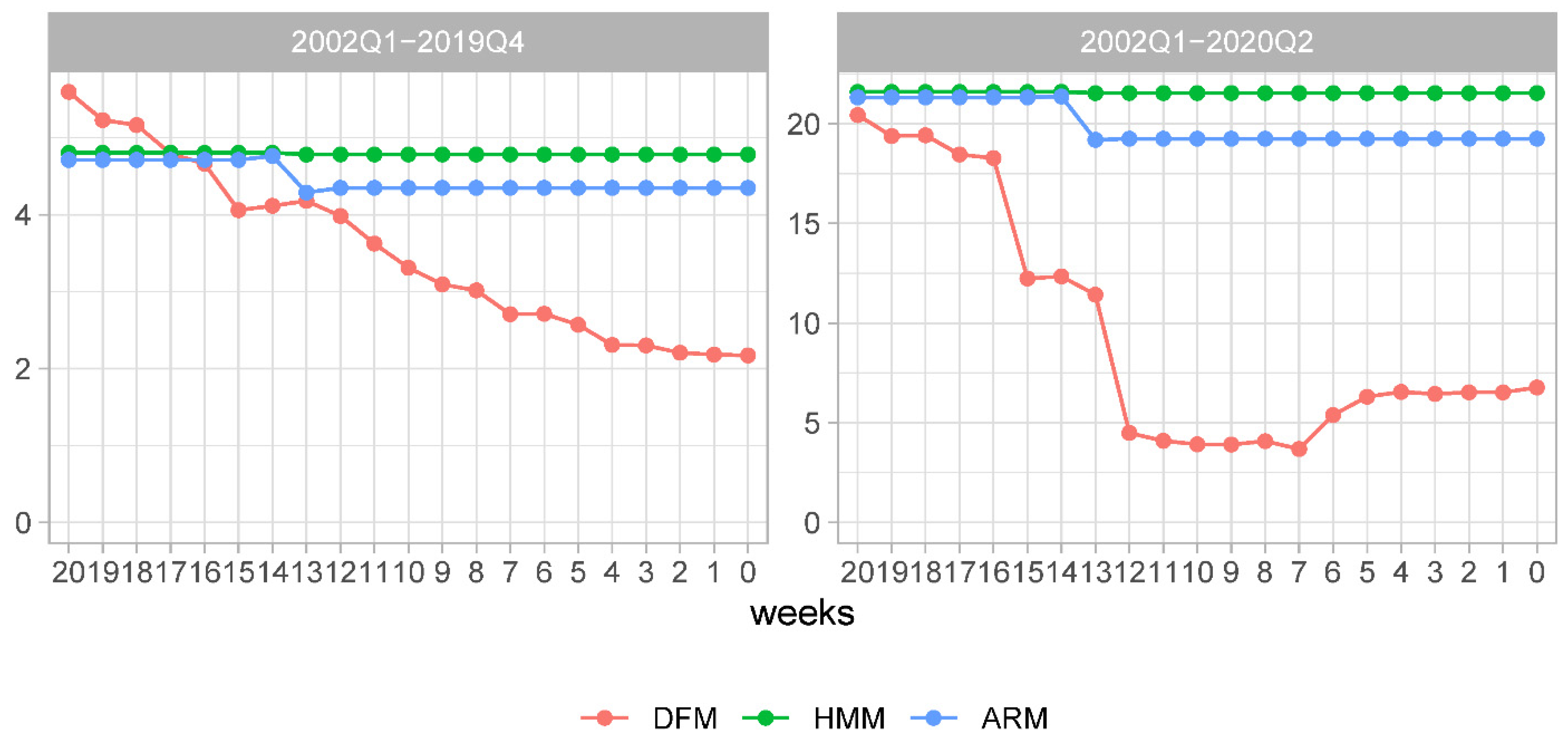
First, we address differences in MSFEs brought about by extending the sample by the COVID recessionary period. The evolution of MSFE at each forecast origin for each of the three models under scrutiny is shown for the pre-COVID and full samples in the left and right panels in Figure 4, respectively. Upon comparing these two plots, it becomes evident that the average squared forecast error substantially increased at every forecast origin and for every model. We also observe that at the earlier forecast origins the relative model ranking has changed. In the pre-COVID period, the univariate benchmark models were characterized by lower MSFE than the NY FED model. In the full sample, this advantage in forecast accuracy of the benchmark models disappeared.

One more detail deserves attention. In the pre-COVID period, the MSFE of the DFM showed a clear downward trending behavior, implying increasing forecast accuracy as more information was incorporated into the model. In the full sample, this pattern is no longer observed. In fact, the most accurate predictions are made for the forecasts made about 7–12 weeks before advance GDP releases. Forecasts made at shorter forecast horizons are characterized by increasing MSFE values. 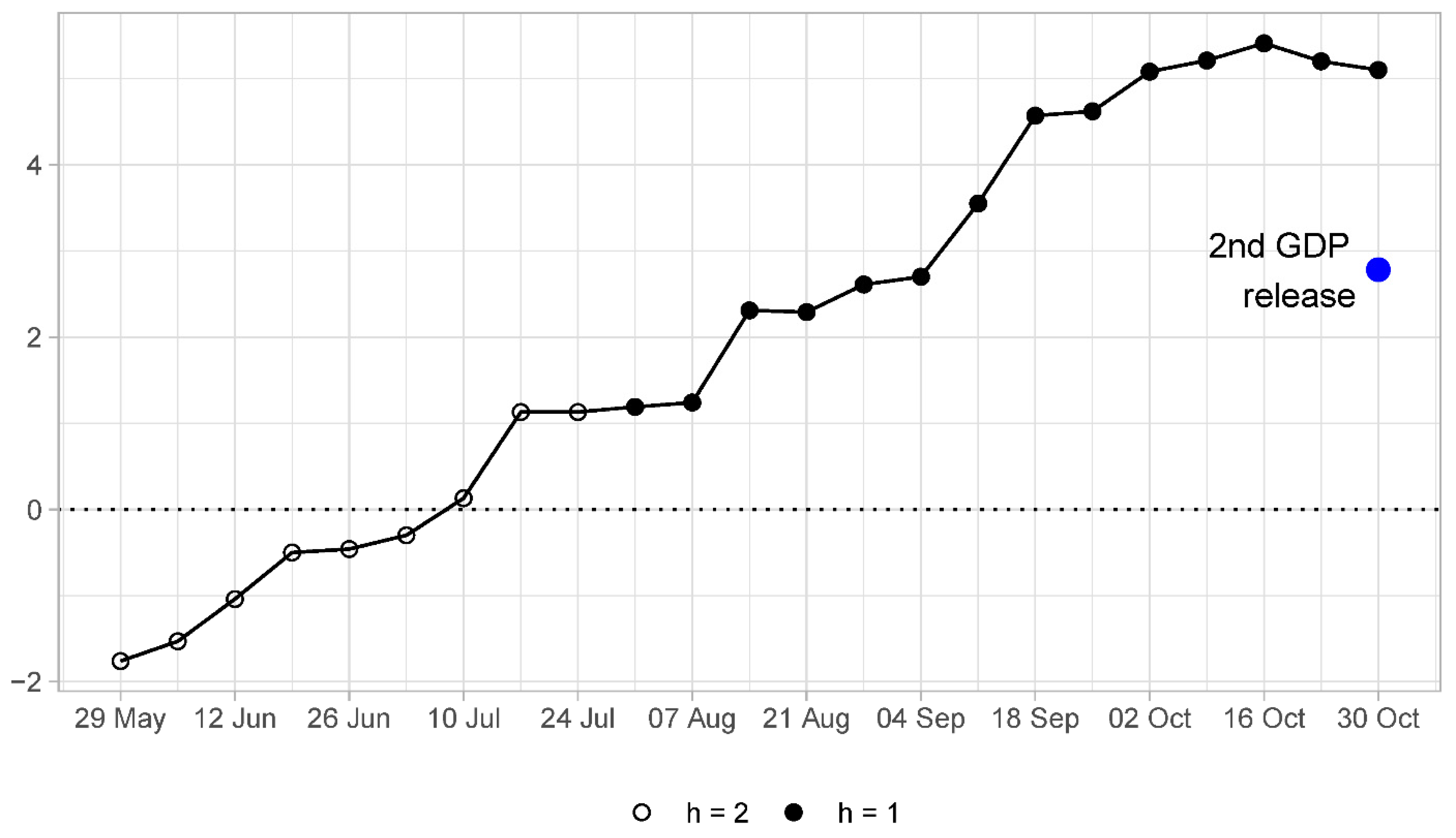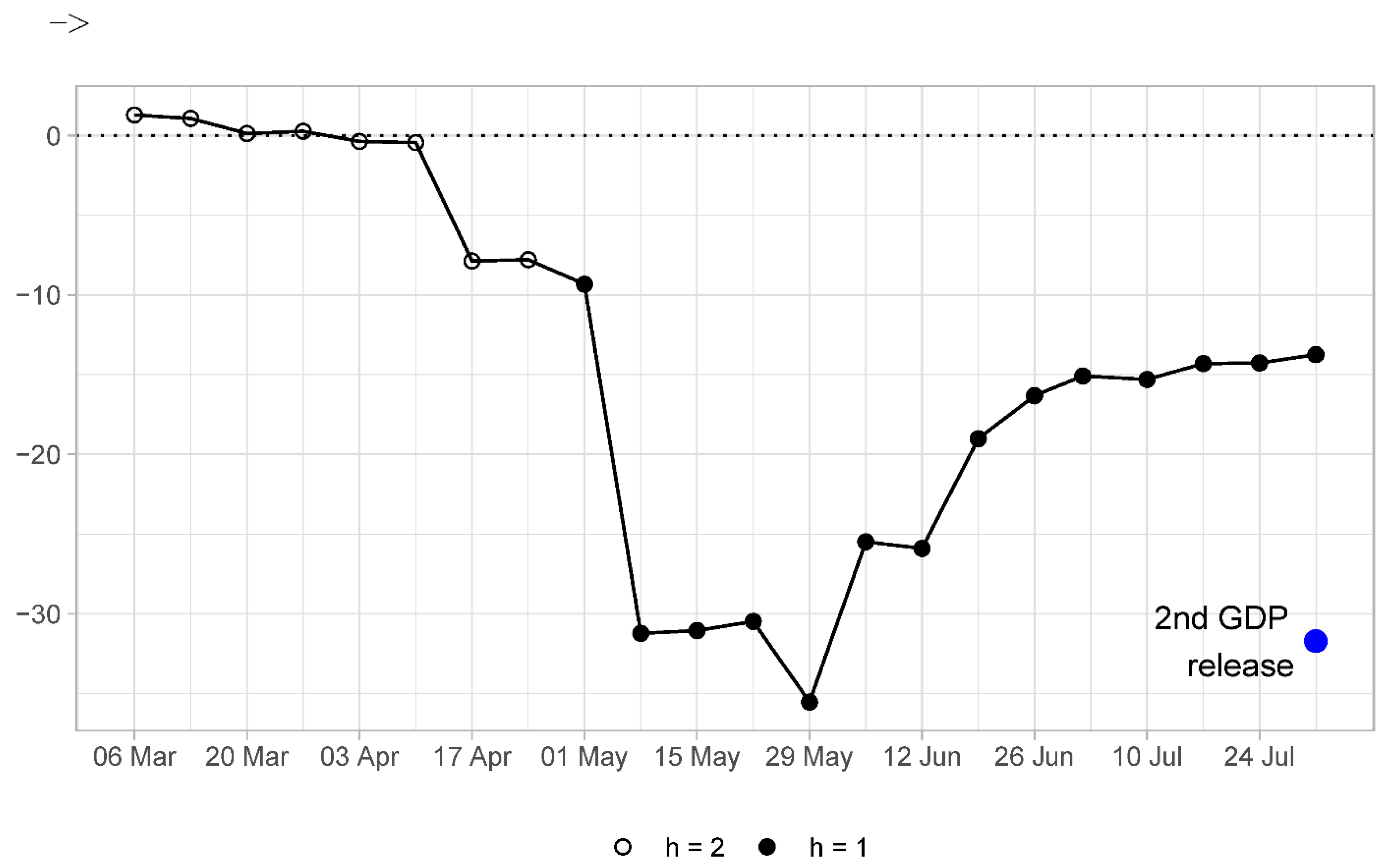An explanation for such observation can be found in Figure 2 where the sequence of nowcasts for 2020Q2 is presented. One can observe that, at the forecast origins of 7–12 weeks, the nowcasts are very close to the GDP outturn, whereas this is not the case for nowcasts made either earlier or later than that. In short, this example illustrates that a single data point can have a rather large influence on the measures of forecast accuracy based on averages of squared forecast errors.

Comparative forecasting performance of the benchmark models deserves a special mention. As can be seen in Figure 4, when evaluated for the full sample (either with or without the COVID period), the ARM produces lower MSFE values than the HMM. At first glance, this observation should support the choice of the autoregressive model as the harder-to-beat benchmark model. However, when one examines the relative MSFE_ARM/HMM reported in Table 2, it becomes evident that during the expansionary phase the MSFE values of the ARM are up to 20% higher than those of the HMM. It is only during recessions when losses in forecast accuracy during expansions relative to the historical mean model are overcompensated by the respective gains for the autoregressive model. This implies that the HMM is a harder-to-beat benchmark during the expansions that take a lion’s share of observations in our sample. This is actually the main reason why the relative measures of forecast accuracy are reported with respect to the historical mean model in this study.

Motivated by this conclusion, we present evolution rMSFE DFM/HMM for the samples without and with COVID observations in Figure 5. The overall conclusion that can be tentatively made is very comforting for the NY FED nowcasting model. The reduction in MSFEs, when compared to that of the HMM, is up to 55% for the pre-COVID forecast evaluation sample and about 80% for the full sample under scrutiny.

Another dimension for the analysis of the predictive ability of the NY FED nowcasting model is to compare the MSFE values for the expansionary and recessionary periods. Chauvet and Potter (2013) observe that during recessions it is harder to make forecasts in the sense that forecast errors tend to be larger than those observed during expansions. The corresponding MSFE values are shown in Figure 6. In the left panel of the figure, we report the evolution of the MSFE for expansionary (2002Q1–2007Q3 and 2009Q3–2019Q4) and recessionary samples (2007Q4–2009Q2) in the pre-COVID period. In the right panel of the figure, we report the evolution of the MSFE for the expansionary (2002Q1–2007Q3 and 2009Q3–2019Q4) and recessionary samples (2007Q4–2009Q2 and 2020Q1–2020Q2) in the full period.

For the pre-COVID sample, one can observe the pattern that largely conforms to the observation made by Chauvet and Potter (2013). At the earlier forecast origins, the forecasts are less precise during the GFC than during the expansionary phases. At the same time, for the forecasts made less than three weeks ahead of the advance GDP estimate releases, the forecasting accuracy during the GFC and expansions is very similar. However, the latter observation can no longer be confirmed when one compares the MSFEs computed for both the GFC and COVID recessionary periods with the MSFE computed for the expansionary period. As can be seen from the right panel of Figure 6, at all forecast origins, forecasts of GDP growth during the recessions are less precise than those during the expansions.

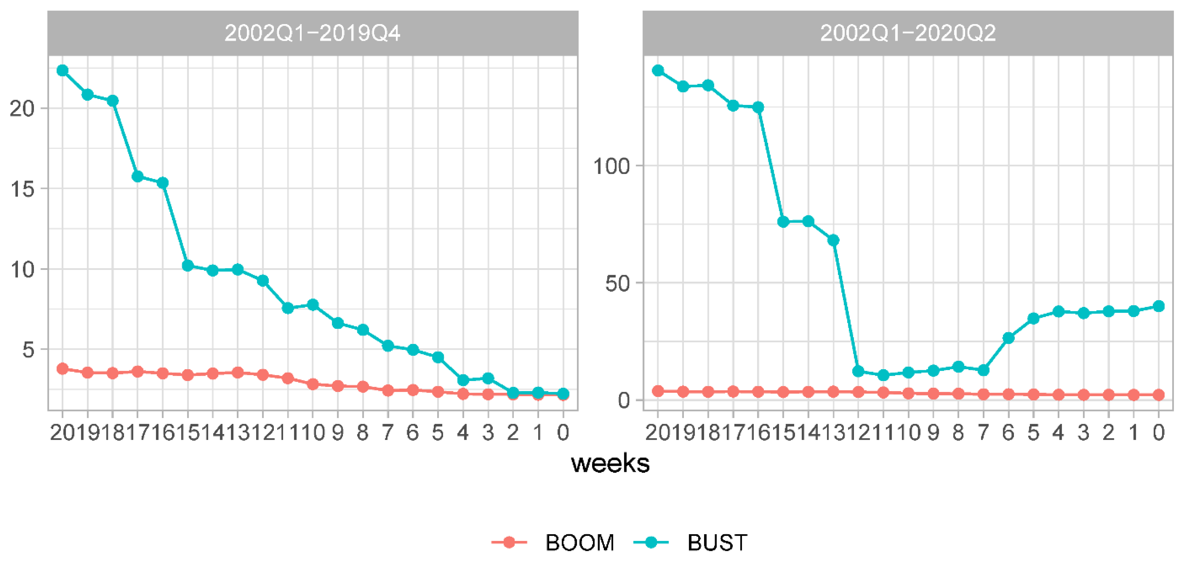
More importantly, given such large differences in nominal measures of forecast accuracy during recessions and expansions, it is worthwhile verifying whether there are noticeable differences in the relative measures. In Figure 7, we plot the evolution of the relative MSFE of the NY FED model and the historical mean model rMSFE_DFM/HMM separately for the recessionary and expansionary periods. The left panel shows the results for the pre-COVID sample and the right panel—for the sample extended with the COVID recessionary period.

In both panels of Figure 7, one can observe a very pronounced asymmetry in the relative forecast accuracy between the DFM and HMM. During expansions, the HMM model produces more precise forecasts made at forecast origins longer than four weeks ahead of advance GDP releases. Only where forecasts are made less than four weeks ahead of advance GDP releases, the forecast accuracy of both models becomes very similar. Given the timing of a typical advance GDP release, this corresponds to the forecast origins at the end of the last month of a targeted quarter and during the weeks of the first month after the end of the targeted quarter. This observation is consistent with that made by Chauvet and Potter (2013), i.e., simple univariate models are robust forecasting devices during expansions; see also Siliverstovs (2020a) for an assessment of the predictive ability of the model of Carriero et al. (2015) for US GDP growth during expansions and recessions. At the same time, during economic crisis periods, the NY FED nowcasting model produces much more accurate forecasts than the historical mean model.

At this point, it is instructive to compare rMSFE_DFM/HMM shown in Figure 5 for the full sample (excluding or including the COVID recession) with the above values of rMSFE_DFM/HMM shown in Figure 7. As can be seen, the advantages of the more sophisticated model over the very simple benchmark model reported for the full sample are brought about by rather few observations during economic crises, be it only the Great Financial Crisis or both the GFC and COVID pandemic. Hence, when one ignores this asymmetry in the forecasting performance of the models during business cycles, the forecasting ability of a more sophisticated model tends to be severely overstated during expansions. In this sense, recessions serve as the breadwinner for forecasters devoted to developing evolved models—a point that was made by Siliverstovs and Wochner (2021)/Siliverstovs and Wochner (2019) after a comprehensive and systematic evaluation of forecastability of more than 200 US time series during expansions and recessions.

6.2. Recursive Estimates of the Relative Forecasting Accuracy

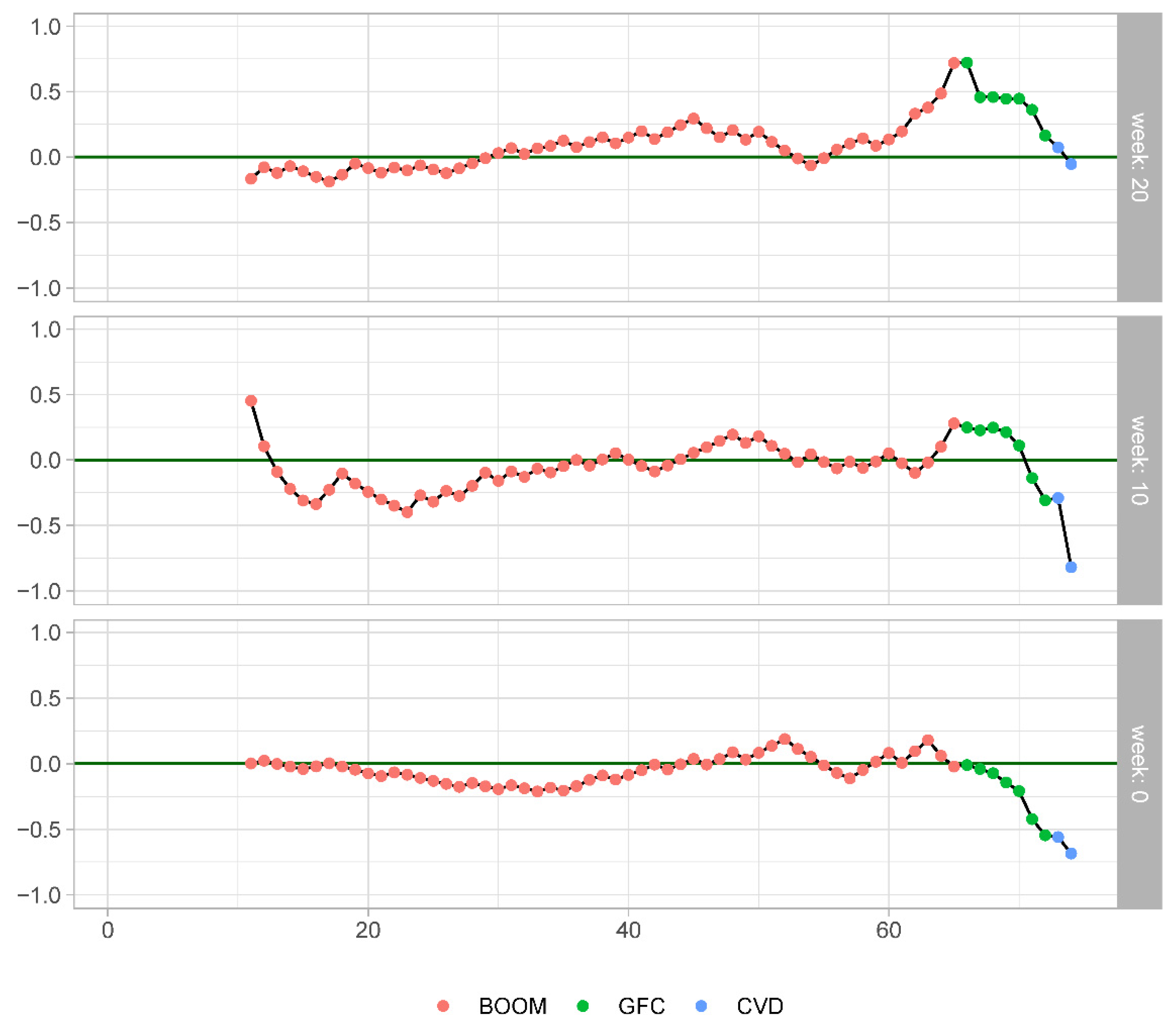
In this section, we present an analysis of the relative forecasting accuracy of the NY FED dynamic factor model (DFM) and the historical mean model (HMM). The main focus of our analysis is centered around Figures 9 and 11 representing CSSFED DFM/HMM and R²MSFE(+R) recursive measures. The auxiliary plots depicting SFED DFM/HMM in its natural temporal ordering and rearranged by its absolute value within each sub-period (expansionary, GFC, and CVD) are represented in Figures 8 and 10, respectively.

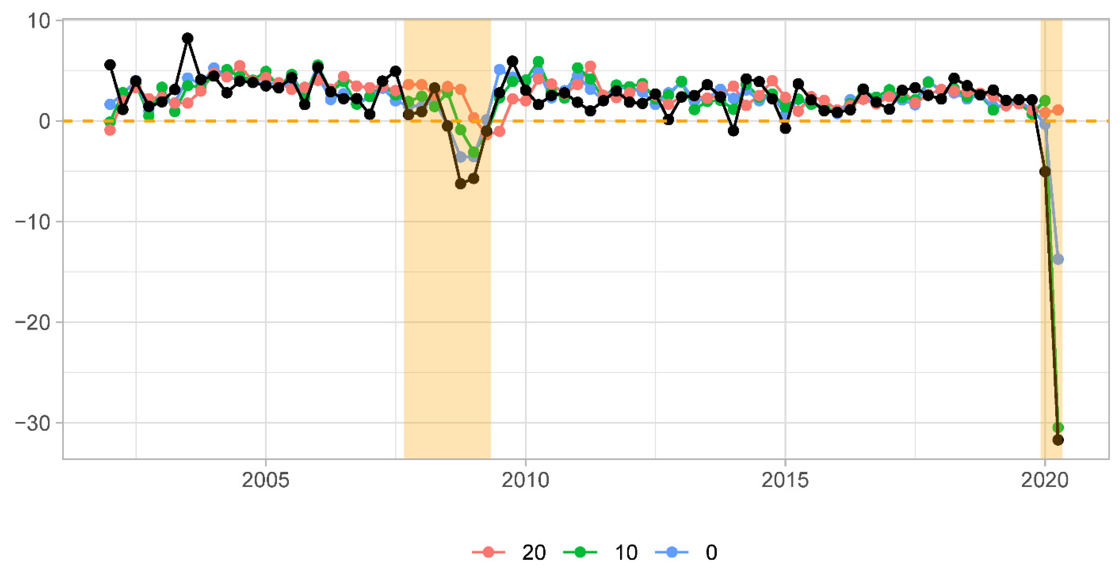
For the sake of brevity and without loss of generalization, we will concentrate on the forecasts made at the three selected forecast origins, namely 20, 10, and 0 weeks ahead of advance GDP estimate releases. Figure 8 depicts the SFED DFM/HMM computed for each out-of-sample forecast evaluation period. As can be seen, there are rather few observations for which we observe substantial differences in the forecast accuracy at the 20-week forecast origin. Less so at the other two forecast origins. Please note that during the COVID pandemic in 2020Q2 there is the largest SFED in our sample. As expected during the GFC, we also observe substantial differences in forecast accuracy between these two models.

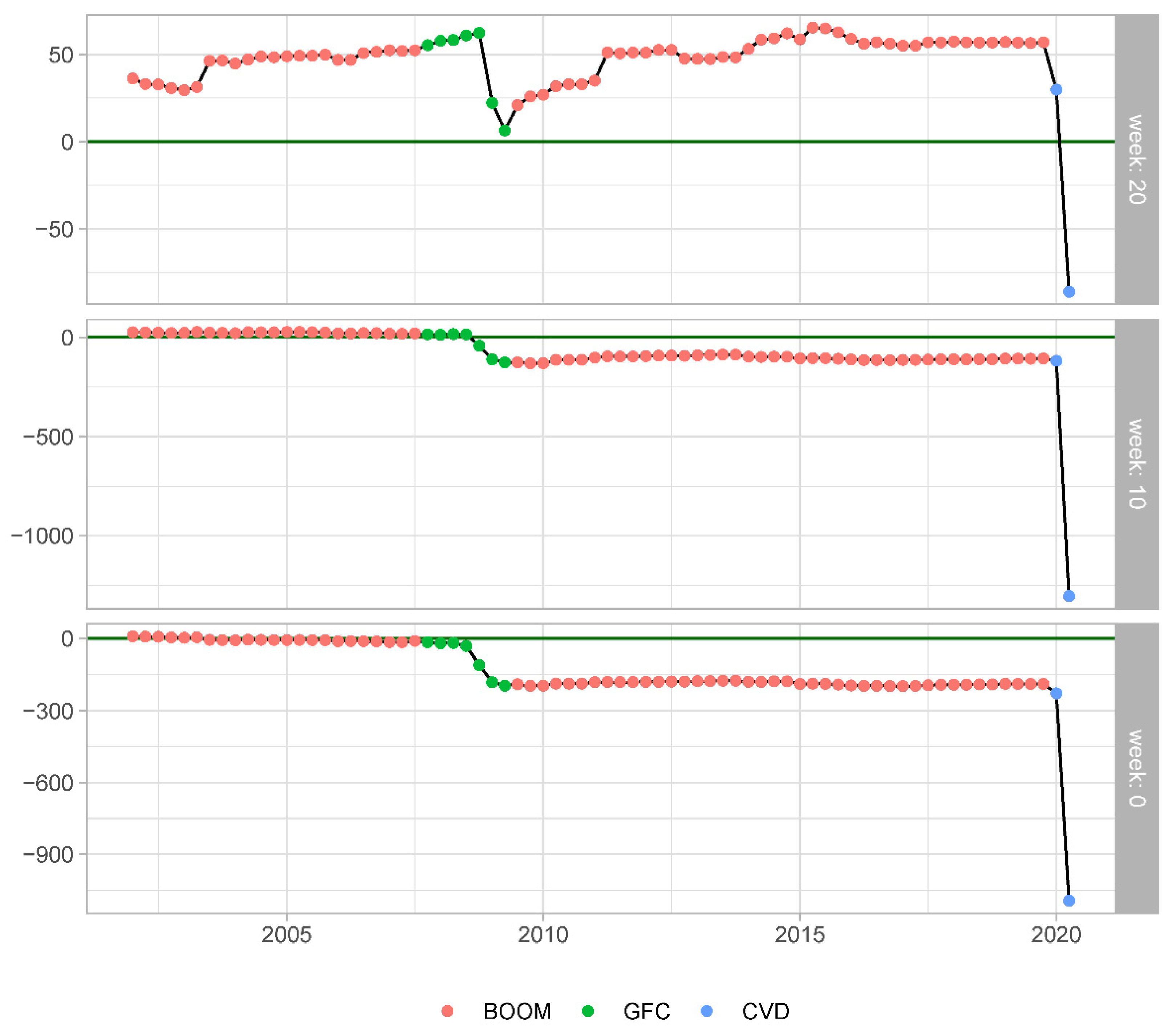
The raw plots of SFED DFM/HMM are informative in pointing out that the models’ forecasting accuracy varies from observation to observation and it tends to be more pronounced during periods of economic distress. However, a simple operation makes these differences informative about changes in the relative ranking of the models, based on their forecasting performance. The resulting cumulative sums of these SFED DFM/HMM are shown in the respective panels of Figure 9. Points above the zero line indicate that up until this observation the DFM produced on average higher squared forecast errors than the HMM. Points below the zero line indicate the opposite.

As for the forecasts made at the 20-week origin (see the upper panel of Figure 9), we can conclude that, based on the evidence from all but one observation (2020Q2), the forecast accuracy produced by the HMM was superior to that of the DFM. It was only the latest observation in our forecast evaluation sample that was the game changer reversing the conclusion in favour of the DFM over the HMM. This is a good example when one observation leads to complete overhaul of the models’ relative ranking based on their average forecasting performance. From the middle panel of Figure 9, we can infer that the conclusion on the superior average forecasting ability of the HMM over DFM reversed much earlier, i.e., during the GFC period. In any case, for the 10- and 0-week forecast origins, the observation in 2020Q2 strongly reinforces the evidence of the superior average forecasting accuracy of the NY FED nowcasting model that first surfaced during the GFC.

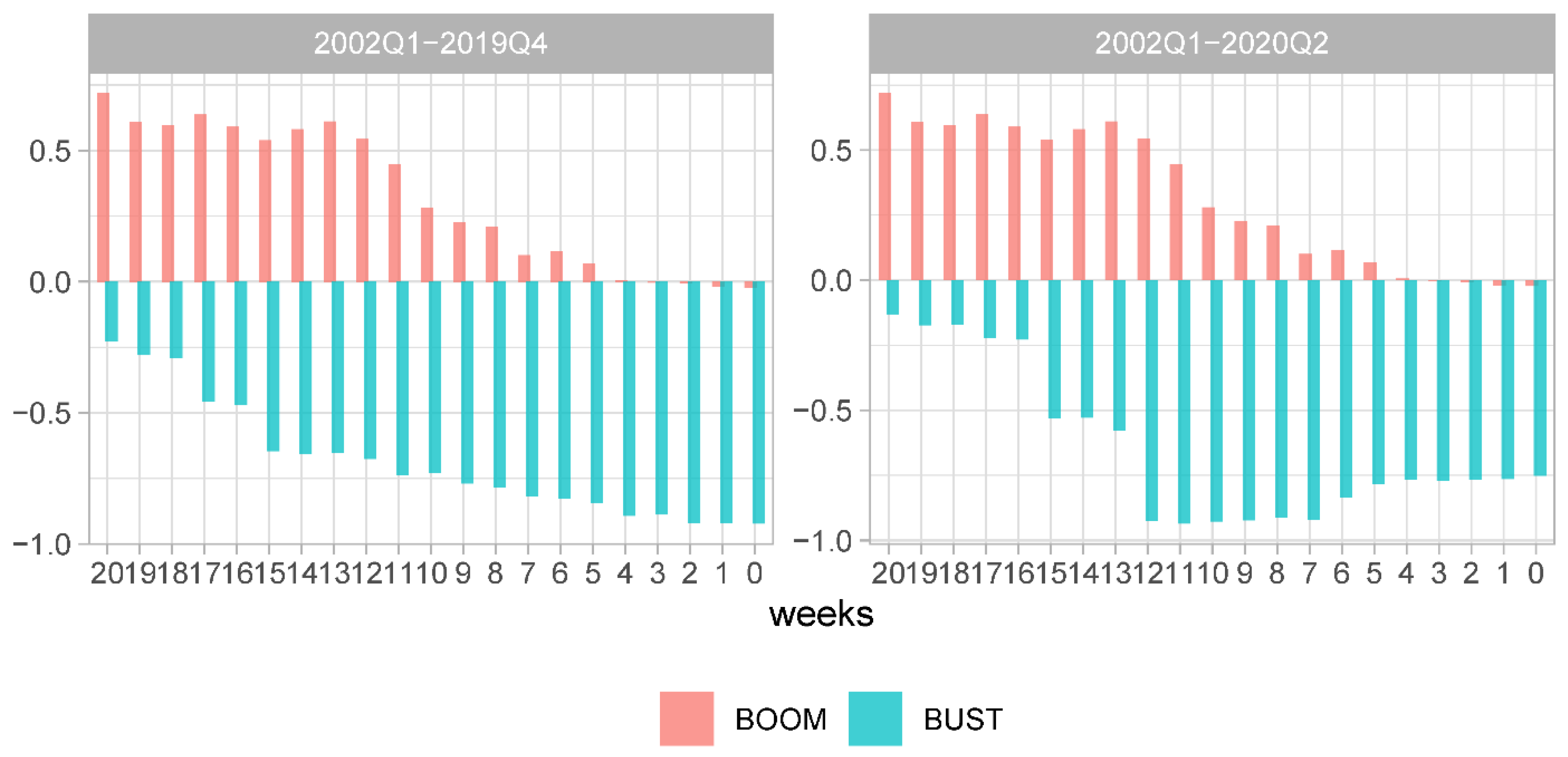
Last but not least, we conclude the analysis of relative predictive ability using the R²MSFE(+R) of Siliverstovs (2020b). The R²MSFE(+R) allows to directly track the evolution of the rMSFE DFM/HMM, as for its computation one adds more and more observations of increasing intensity that is measured in terms of absolute values of SFED, |SFED_t|. One option is to report R²MSFE(+R) based on the reordered observations purely by the magnitude of |SFED_t| in the ascending order. We, however, apply a slight modification in rearranging the observations capitalising on the knowledge of the expansionary and recessionary phases of the business cycle in our data. We present the R²MSFE(+R) in Figure 10 that is based on the observations rearranged by the magnitude of |SFED_t| in ascending order within each of the three sub-samples: the expansions (2002Q1–2007Q3 and2009Q3–2019Q4), the GFC period (2007Q4–2009Q2), and the COVID period (2020Q1–2020Q2). 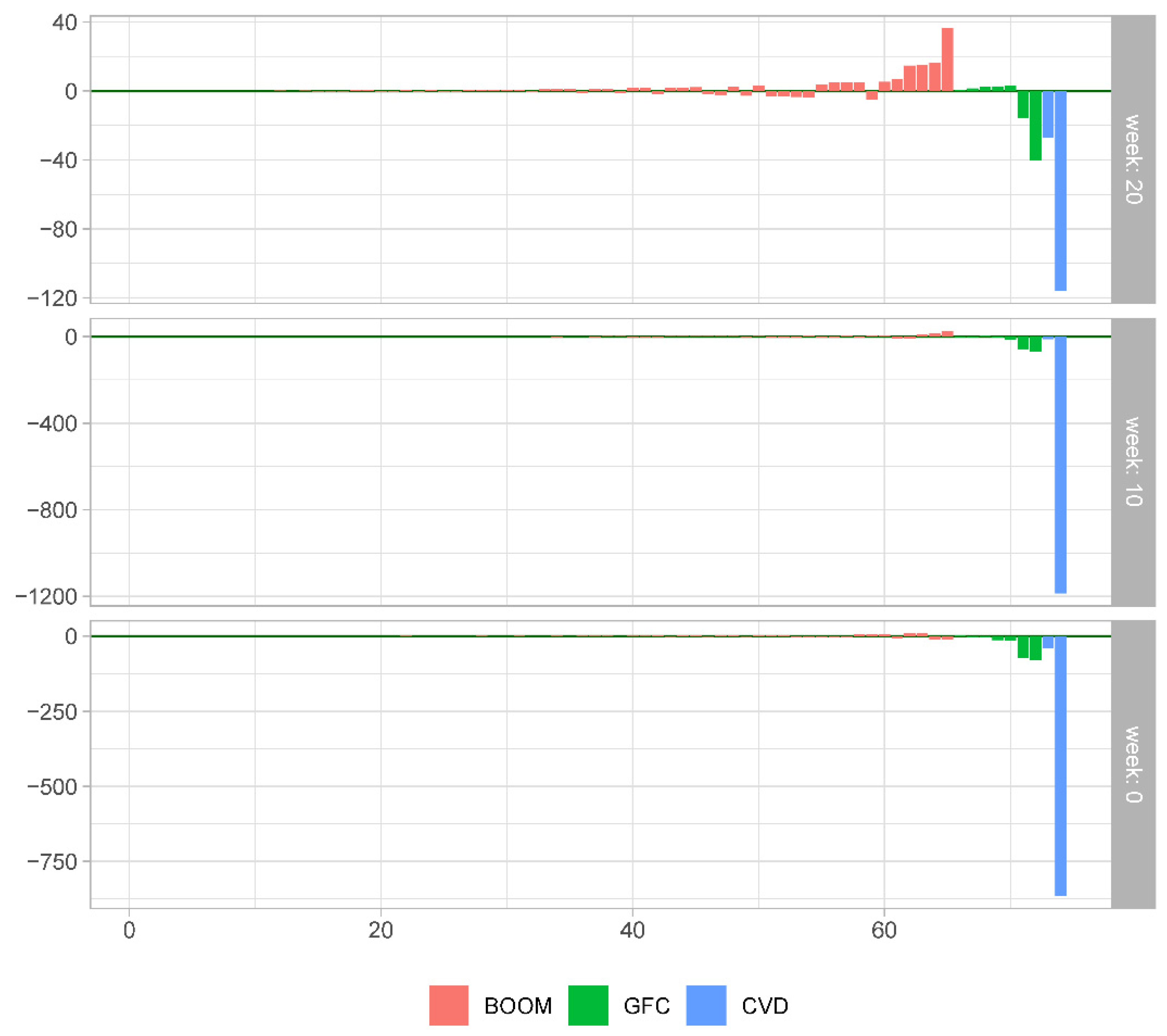The main advantage of visually presenting the results in this way is that they are directly comparable to the numerical results reported in Table 2. The underlying SFEDs, rearranged in the ascending order according to its modulus within the three sub-periods (expansionary, the GFC, and COVID periods), are shown in Figure 11.

The R²MSFE(+R) calculated using the forecasts for the three selected forecast origins are shown in Figure 10. These sequences visually display asymmetry in the relative forecasting ability of the dynamic factor and historical mean models during different sub-samples. As for the expansionary period, we can clearly observe that the HMM, on average, produces lower squared forecast errors than its sophisticated counterpart at the forecast origins that are 20- and 10-weeks ahead of advance GDP releases. The last point in the red sequence in the upper and middle panels of the figures corresponds to the rMSFE reported in Column (3) of Table 2. These values indicate that the MSFE of the DFM model is 71.8% and 28.0% higher than that of the HMM for the forecasts made 20 and 10 weeks before the releases of advance GDP estimates. We can infer from the lower panel of the figure that the rMSFE_DFM/HMM is very close to zero for the forecasts released during the same week when advance GDP estimates are published. In fact, the corresponding entry of −0.022 in Table 2 indicates that the MSFE_DFM is only about 2% lower than the MSFE_HMM during expansions.

The sequence of the green dots shows how the relative MSFE changes if we add observations from the GFC period. The last green dot corresponds to the value of rMSFE reported in Column (1) in Table 2. For the 20-week-ahead forecasts, we can read off the corresponding value of 0.165 which indicates that the HMM average forecast accuracy is superior to that of the DFM, even when the observations from the GFC are taken into account. However, for the shorter forecast horizon of 10 weeks, the corresponding entry is −0.308 indicating changes in the models’ relative ranking brought about by the observations during the GFC period. This perfectly illustrates how excessive gains in the forecasting ability during the Great Recession, accrued by the more sophisticated model, can overcompensate for the forecast accuracy losses during much longer periods of economic expansion. As for the forecasts released during the same week as advance GDP releases, the relevant value of −0.546 in Table 2 signals a reduction of about 55% in MSFE brought about by the DFM.

Finally, the blue dots indicate how rMSFE_DFM/HMM changes if the two remaining observations (2020Q1–2020Q2) are added to the sample. The last dots in these sequences correspond to the entries in Column (7) of Table 2 for the DFM model. As discussed above, addition of these observations changes the relative ranking of the models for 20-week-ahead forecasts, now indicating a reduction of about 5.4% in MSFE brought about by the DFM, and substantially lowers the relative MSFE for the forecasts made at shorter forecast horizons. The corresponding reductions in MSFE are 81.8% and 68.6% relative to those of the HMM.

7. Conclusions

In this study, we analyze the predictive performance of the dynamic factor model (DFM) developed and maintained at the NY FED. In contrast to many forecasting exercises that were carried out on the past historical data vintages, this project publishes forecasts in a do-it-as-you-go manner and, therefore, is void of data snooping biases. This fact allows us to evaluate the genuine forecasting ability of the econometric model in question, not the least, during the unfolding COVID-19 pandemic when the uncertainty about the current economic conditions is substantially elevated compared to the tranquil times and the demand for accurate assessment of the current state of the economy is especially acute.

The dataset that we analyze comprises US GDP quarterly growth forecasts made in real time squared since 2016 and forecasts calculated backwards during 2002–2015 using historical data vintages. We summarize the nominal and relative accuracy of the DFM forecasts made at 21 weekly forecast origins. The earliest forecast origin precedes releases of advance GDP estimates by 20 weeks, next forecast origin—by 19 weeks, and so on until the week when the advance GDP estimate is released for the targeted quarter. The DFM forecast accuracy is compared with that of two benchmark models: a historical mean model (HMM) and autoregressive model of order (2), ARM.

The main contribution to the forecasting literature is that we analyze the DFM predictive performance during the whole period as well as separately during its expansionary and recessionary sub-periods. The recessionary sub-period includes two distinct periods: the Great Financial Crisis (2007Q4–2009Q2) and the first two quarters of the unfolding COVID-19 pandemic (2020Q1–2020Q2). In doing so, we intend to verify whether the conclusions of Chauvet and Potter (2013) on the asymmetric predictive ability of a wide range of modern macroeconometric models also applies to the NY FED nowcasting model.

Our main conclusion is that we indeed observe a very strong variation in the forecasting ability of the DFM across the business cycle phases. This conclusion is supported when one compares the predictive performance during the pre-COVID period, where there is only one recessionary period (GFC) in our sample, and it is even further reinforced when the latest observations from the COVID pandemic period are included in the analysis. As for the expansionary period, we find that at longer forecast horizons accuracy of the DFM predictions is inferior to that of the historical mean model. It is only at the forecast origins less than 4 weeks ahead of advance GDP releases where both the sophisticated and the naive benchmark models deliver similar forecasting accuracy. On the contrary, the DFM delivers superior forecast accuracy during the recessionary quarters.

Our analysis also demonstrates that the widespread practice of reporting the measures of forecast accuracy, based on average squared forecast errors (and their differences) over longer periods that include both expansionary and recessionary phases of business cycles, are prone to deliver a biased assessment of the models’ nominal and relative forecasting ability. Typically, since the relative gains in the forecasting accuracy of a more sophisticated model during recessions significantly outweigh the relative losses during expansions, the results of averaging across both expansions and recessions tend to artificially exaggerate the predictive ability of a more sophisticated model relative to naive benchmarks both for the period as a whole and during its expansionary sub-sample.

In order to avoid such misrepresentation of the results of a forecasting exercise, it is advisable to complement the measures of forecasting ability reported for the whole sample with results reported for more homogeneous sub-samples, e.g., expansions and recessions. Additional information regarding the models’ relative forecasting ability can be provided by recursive measures of forecasting accuracy such as CSSFED of Welch and Goyal (2008) and R²MSFE(+R) of Siliverstovs (2020b). The recursive measures dissect the relative predictive performance of the competing models’ observation by observation and alleviate the gauging leverage of one or more observations on the models’ relative ranking.

References

1. Aarons, Grant, Daniele Caratelli, Domenico Giannone, Argia Sbordone, and Andrea Tambalotti. 2016. Just Released: Introducing the New York Fed Staff Nowcast. Federal Reserve Bank of New York Liberty Street Economics (blog). Available online: https://libertystreeteconomics.newyorkfed.org/2016/04/just-released-introducing-the-frbny-nowcast.html (accessed on 21 February 2021).
2. Adams, Patrick, Brandyn Bok, Daniele Caratelli, Domenico Giannone, Eric Qian, Argia Sbordone, Camilla Schneier, and Andrea Tambalotti. 2018. Opening the Toolbox: Computer Code for the Nowcast. Federal Reserve Bank of New York, Liberty Street Economics. Available online: http://libertystreeteconomics.newyorkfed.org/2018/08/opening-the-toolbox-the-nowcasting-code-on-github.html (accessed on 21 February 2021).
3. Adams, Patrick, Domenico Giannone, Eric Qian, and Argia Sbordone. 2019. Just Released: Historical Reconstruction of the New York Fed Staff Nowcast, 2002-15. Federal Reserve Bank of New York, Liberty Street Economics. Available online: https://libertystreeteconomics.newyorkfed.org/2019/07/just-released-historical-reconstruction-of-the-new-york-fed-staff-nowcast-2002-15.html (accessed on 21 February 2021).
4. Alessi, Lucia, Eric Ghysels, Luca Onorante, Richard Peach, and Simon Potter. 2014. Central Bank Macroeconomic Forecasting During the Global Financial Crisis: The European Central Bank and Federal Reserve Bank of New York Experiences. Journal of Business & Economic Statistics 32: 483–500. [Google Scholar]
5. Babii, Andrii, Eric Ghysels, and Jonas Striaukas. 2019. Machine Learning Time Series Regressions with an Application to Nowcasting. Available online: https://papers.ssrn.com/sol3/papers.cfm?abstract_id=3503191 (accessed on 21 February 2021).
6. Banbura, Marta, Domenico Giannone, and Lucrezia Reichlin. 2011. Nowcasting. In Oxford Handbook on Economic Forecasting. Edited by M. P. Clements and D. F. Hendry. Amsterdam: Elsevier, Chp. 7. pp. 193–224. [Google Scholar]
7. Bok, Brandyn, Daniele Caratelli, Domenico Giannone, Argia Sbordone, and Andrea Tambalotti. 2018. Macroeconomic Nowcasting and Forecasting with Big Data. Annual Review of Economics 10: 615–43. [Google Scholar] [CrossRef] [Green Version]
8. Cai, Michael, Marco Del Negro, Marc. P. Giannoni, Abhi Gupta, Pearl Li, and Erica Moszkowski. 2019. DSGE forecasts of the lost recovery. International Journal of Forecasting 35: 1770–89. [Google Scholar] [CrossRef] [Green Version]
9. Carriero, Andrea, Todd E. Clark, and Massimiliano Marcellino. 2015. Realtime nowcasting with a bayesian mixed frequency model with stochastic volatility. Journal of the Royal Statistical Society: Series A (Statistics in Society) 178: 837–62. [Google Scholar] [CrossRef] [PubMed]
10. Chauvet, Marcelle, and Simon Potter. 2013. Forecasting output. In Handbook of Forecasting. Edited by G. Elliott and A. Timmermann. Amsterdam: North Holland, vol. 2, pp. 1–56. [Google Scholar]
11. Cimadomo, Jacopo, Domenico Giannone, Michele Lenza, Andrej Sokol, and Francesca Monti. 2020. Nowcasting with Large Bayesian Vector Autoregressions. Working Paper Series 2453; Frankfurt: European Central Bank. [Google Scholar]
12. Foroni, Claudia, Massimiliano Marcellino, and Christian Schumacher. 2015. Unrestricted mixed data sampling (midas): Midas regressions with unrestricted lag polynomials. Journal of the Royal Statistical Society: Series A (Statistics in Society) 178: 57–82. [Google Scholar] [CrossRef]
13. Geweke, John, and Gianni Amisano. 2010. Comparing and evaluating Bayesian predictive distributions of asset returns. International Journal of Forecasting 26: 216–30. [Google Scholar] [CrossRef]
14. Giannone, Domenico, Argia Sbordone, and Andrea Tambalotti. 2017. Hey, Economist! How Do You Forecast the Present? New York: Federal Reserve Bank of New York Liberty, Available online: http://libertystreeteconomics.newyorkfed.org/2017/06/hey-economist-how-do-you-forecast-the-present.html (accessed on 21 February 2021).
15. Giannone, Domenico, Lucrezia Reichlin, and David Small. 2008. Nowcasting: The real-time informational content of macroeconomic data. Journal of Monetary Economics 55: 665–76. [Google Scholar] [CrossRef]
16. R Core Team. 2012. R: A Language and Environment for Statistical Computing. Vienna: R Foundation for Statistical Computing, ISBN 3-900051-07-0. [Google Scholar]
17. Rossi, Barbara. 2013. Advances in Forecasting under Instability. Amsterdam: Elsevier, vol. 2, chp. 21. pp. 1203–324. [Google Scholar]
18. Siliverstovs, Boriss. 2012. Keeping a Finger on the Pulse of the Economy: Nowcasting Swiss GDP in Real-Time Squared. KOF Working Papers 12-302. Zürich: KOF Swiss Economic Institute, ETH Zurich. [Google Scholar]
19. Siliverstovs, Boriss. 2017. Dissecting models’ forecasting performance. Economic Modelling 67: 294–99. [Google Scholar] [CrossRef] [Green Version]
20. Siliverstovs, Boriss. 2020a. Assessing nowcast accuracy of US GDP growth in real time: The role of booms and busts. Empirical Economics 58: 7–27. [Google Scholar] [CrossRef]
21. Siliverstovs, Boriss. 2020b. Gauging the Effect of Influential Observations on Measures of Relative Forecast Accuracy in Post-COVID-19 era: An Application to Nowcasting Euro Area GDP Growth. Unpublished Manuscript. [Google Scholar]
22. Siliverstovs, Boriss, and Daniel Wochner. 2021. State-dependent evaluation of predictive ability. Journal of Forecasting 40: 547–74. [Google Scholar] [CrossRef]
23. Siliverstovs, Boriss, and Daniel Wochner. 2019. Recessions as Breadwinner for Forecasters State-Dependent Evaluation of Predictive Ability: Evidence from Big Macroeconomic US Data. KOF Working Papers 19-463. Zürich: KOF Swiss Economic Institute, ETH Zurich. [Google Scholar]
24. Siliverstovs, Boriss, and Konstantin. A. Kholodilin. 2012. Assessing the real-time informational content of macroeconomic data releases for now-/forecasting GDP: Evidence for Switzerland. Jahrbücher für Nationalökonomie und Statistik 232: 429–44. [Google Scholar]
25. Stock, James H., and Mark W. Watson. 2002. Macroeconomic forecasting using diffusion indexes. Journal of Business and Economic Statistics 20: 147–62. [Google Scholar] [CrossRef] [Green Version]
26. Welch, Ivo, and Amit Goyal. 2008. A comprehensive look at the empirical performance of equity premium prediction. Review of Financial Studies 21: 1455–508. [Google Scholar] [CrossRef]
Figure 1. Sequence of weekly nowcasts for 2009Q3.
Econometrics 09 00011 g001
Figure 2. Sequence of weekly nowcasts for 2020Q2.
Econometrics 09 00011 g002
Figure 3. GDP growth: Actual (second release) and forecasts. Forecasts at selected forecast origins are shown. In the legend, 20 and 10 indicate the number of weeks ahead of releases of advance GDP estimates. The remaining forecast sequence, labelled as 0, corresponds to the forecasts made during the same week when advance GDP estimates were published.
Econometrics 09 00011 g003
Figure 4. MSFEs reported for the pre-COVID and full samples.
Econometrics 09 00011 g004
Figure 5. Relative MSFEs (DFM/HMM) reported for the pre-COVID and full samples.
Econometrics 09 00011 g005
Figure 6. MSFEs (DFM) in expansions/recessions, reported for the pre-COVID and full samples.
Econometrics 09 00011 g006
Figure 7. rMSFEs (DFM/HMM) in expansions/recessions, reported for the pre-COVID and full samples.
Econometrics 09 00011 g007
Figure 8. SFEDDFM/HMM computed for selected forecast origins, 20, 10, and 0 weeks ahead of advance GDP estimate releases.
Econometrics 09 00011 g008
Figure 9. CSSFEDDFM/HMM computed for selected forecast origins, 20, 10, and 0 weeks ahead of advance GDP estimate releases.
Econometrics 09 00011 g009
Figure 10. R2MSFE(+R)DFM/HMM computed for selected forecast origins, 20, 10, and 0 weeks ahead of advance GDP estimate releases.
Econometrics 09 00011 g010
Figure 11. SFEDDFM/HMM rearranged by its modulus computed for selected forecast origins, 20, 10, and 0 weeks ahead of advance GDP estimate releases.
Econometrics 09 00011 g011