Using the SARIMA Model to Forecast the Fourth Global Wave of Cumulative Deaths from COVID-19: Evidence from 12 Hard-Hit Big Countries

Abstract

The COVID-19 pandemic is a serious threat to all of us. It has caused an unprecedented shock to the world’s economy, and it has interrupted the lives and livelihood of millions of people. In the last two years, a large body of literature has attempted to forecast the main dimensions of the COVID-19 outbreak using a wide set of models. In this paper, I forecast the short- to mid-term cumulative deaths from COVID-19 in 12 hard-hit big countries around the world as of 20 August 2021. The data used in the analysis were extracted from the Our World in Data COVID-19 dataset. Both non-seasonal and seasonal autoregressive integrated moving averages (ARIMA and SARIMA) were estimated. The analysis showed that: (i) ARIMA/SARIMA forecasts were sufficiently accurate in both the training and test set by always outperforming the simple alternative forecasting techniques chosen as benchmarks (Mean, Naïve, and Seasonal Naïve); (ii) SARIMA models outperformed ARIMA models in 46 out 48 metrics (in forecasting future values), i.e., on 95.8% of all the considered forecast accuracy measures (mean absolute error [MAE], mean absolute percentage error [MAPE], mean absolute scaled error [MASE], and the root mean squared error [RMSE]), suggesting a clear seasonal pattern in the data; and (iii) the forecasted values from SARIMA models fitted very well the observed (real-time) data for the period 21 August 2021–19 September 2021 for almost all the countries analyzed. This article shows that SARIMA can be safely used for both the short- and medium-term predictions of COVID-19 deaths. Thus, this approach can help government authorities to monitor and manage the huge pressure that COVID-19 is exerting on national healthcare systems.

1. Introduction

The COVID-19 pandemic is one of the most severe and dangerous challenges that the world has faced. As a result, the human and socio-economic costs of the COVID-19 pandemic have been dramatically high. As of 20 August 2021, the global death toll from COVID-19 had reached more than 4.4 million people, and several countries had effectively entered the fourth wave of the pandemic (Worldometer 2021). In fact, the virus that caused COVID-19 has mutated multiple times, resulting in highly alarming and contagious variants, such as Alpha, Beta, Delta, and Gamma, which first appeared in the UK, South Africa, Brazil (and Japan), and India, respectively (Centers for Disease Control and Prevention [CDC] 2021).

In such a situation, it becomes crucial to provide reliable forecasts of the patterns of the pandemic so healthcare facilities and personnel can be managed better. Thus, in the last two years, a wide body of studies has attempted to forecast the main dimensions of the COVID-19 pandemic, such as the number of confirmed cases, deaths, hospitalizations, recovered, and vaccinated.

The most used prediction techniques were the seasonal and non-seasonal autoregressive integrated moving average (SARIMA and ARIMA) models (Alzahrani et al. 2020; Kufel 2020; Sahai et al. 2020; ArunKumar et al. 2021; Katoch and Sidhu 2021; Malki et al. 2021; Roy et al. 2021; Satpathy et al. 2021), machine learning algorithm (Ardabili et al. 2020; Sujatha et al. 2020; Tuli et al. 2020; Wang et al. 2020; Ahmad et al. 2021; Kwekha-Rashid et al. 2021), susceptible-exposed-infectious-recovered (SEIR) approach (Annas et al. 2020; Carcione et al. 2020; Piovella 2020; Engbert et al. 2021; Korolev 2021; Viguerie et al. 2021), and hybrid approaches (Hasan 2020; Pinter et al. 2020; Zheng et al. 2020; Castillo Ossa et al. 2021; Safi and Sanusi 2021; Talkhi et al. 2021).

The aim of this paper is to predict the cumulative deaths related to COVID-19 in 12 hard-hit big countries from 21 August 2021 to 19 September 2021 (that is 30 days), using ARIMA and SARIMA models. The choice of the time window is not random. In fact, even if the ARIMA/SARIMA approach is especially used for short-term predictions, it proved to be suitable and sufficiently accurate also for COVID-19 mid-term forecasts (Khan and Gupta 2020; Alabdulrazzaq et al. 2021; Al-Turaiki et al. 2021; ArunKumar et al. 2021). Thus, a 30-day ahead forecast of COVID-19 deaths seems to be a good balance and allows me to closely link my analysis to the recent literature.

The 12 countries chosen for the analysis are very heterogenous, and they come from four continents (Africa, Asia, and North and South America): Argentina, Bangladesh, Brazil, India, Iran, Mexico, the Philippines, Russia, South Africa, Thailand, the United States (US), and Vietnam.

The rest of this paper is organized as follows. In Section 2, I provide a brief review of the related literature. In Section 3, I present the data used for the forecasting analysis. In Section 4, I discuss the methodology. In Section 5, I present and discuss the results. Finally, in Section 6, I provide some conclusive considerations.

2. Brief Review of the Literature

The ARIMA model, also known as the Box–Jenkins method (Box and Jenkins 1976), is one of the most widely used statistical methods for forecasting stationary time series. It has been extensively employed in many areas of research, including environmental pollution (Sen et al. 2016; Zhang et al. 2018), meteorological factors (Valipour 2015; Liu et al. 2021), financial markets (Chung et al. 2009; Adebiyi et al. 2014), and especially for predicting trends and patterns of infectious disease (Earnest et al. 2005; Gaudart et al. 2009; Li et al. 2012; Kane et al. 2014; Liu et al. 2016; Wang et al. 2018; Singh et al. 2020; Ala’raj et al. 2021). The ARIMA model has very good properties. It is easy to fit and manage, and it is understandable even for non-professional users. It can deal with many common practical situations and complex patterns such as calendar variation, cyclicity, seasonality, trends, external or exogenous interventions, outliers, randomness caused by other factors and/or diseases, and other relevant real aspects of time series (Pack 1990; Barnett and Dobson 2010). Moreover, it does not assume any knowledge of underlying models or structure as do some other forecasting methods (Adebiyi et al. 2014). It simply allows the prediction of a given time series by considering its own lags, i.e., the previous values of the observed time series and the lagged forecast errors.

Table 1 lists 32 studies that used an ARIMA/SARIMA framework to forecast the patterns of infectious diseases over the last 16 years.

Table 1. Thirty-two selected studies on infectious disease forecasting, which used non-seasonal and seasonal ARIMA model.

Authors	Disease	Methodological Approach	Investigated Area
Earnest et al. (2005)	SARS	ARIMA	Singapore
Gaudart et al. (2009)	Malaria	ARIMA, SIRS	Mali
Liu et al. (2011)	HFRS	ARIMA	China
Li et al. (2012)	HFRS	SARIMA	China
Ren et al. (2013)	Hepatitis E	ARIMA, BPNN	Shanghai, China
Kane et al. (2014)	H5N1	ARIMA and RANDOM FOREST	Egypt
Zheng et al. (2015)	Tuberculosis	SARIMA	Xinjiang, China
Wei et al. (2016)	Hepatitis A	SARIMA, GRNN, and SARIMA-GRNN	Heng County, China
Zeng et al. (2016)	Pertussis	SARIMA, ETS	China
Xu et al. (2017)	Mumps	SARIMA	Zibo, China
He and Tao (2018)	Influenza	ARIMA	Wuhan, China
Wang et al. (2018)	Hepatitis B	SARIMA, GM (1,1)	China
Cong et al. (2019)	Influenza	SARIMA	Mainland China
Wang et al. (2019)	Human Brucellosis	ARIMA	Jinzhou, China
Alzahrani et al. (2020)	COVID-19	ARIMA	Saudi Arabia
Cao et al. (2020)	Human Brucellosis	SARIMA	Hebei, China
Ceylan (2020)	COVID-19	ARIMA	France, Italy, Spain
Chintalapudi et al. (2020)	COVID-19	ARIMA	Italy
Hossain et al. (2020)	Dengue fever	ARIMA	Dhaka, Bangladesh
Perone (2020)	COVID-19	ARIMA	Italy
Polwiang (2020)	Dengue fever	ANN, ARIMA, MPR	Bangkok, Thailand
Singh et al. (2020)	COVID-19	ARIMA	15 countries
Tran et al. (2020)	COVID-19	ARIMA	Iran
Yousaf et al. (2020)	COVID-19	ARIMA	Pakistan
Ala’raj et al. (2021)	COVID-19	SEIRD-ARIMA	US
ArunKumar et al. (2021)	COVID-19	ARIMA and SARIMA	16 countries
Li et al. (2021)	Tuberculosis	EEMD-ARIMA-NANN	Tibet
Malki et al. (2021)	COVID-19	SARIMA	20 countries
Perone (2021b)	COVID-19	ETS, NARNN, SARIMA, TBATS, and hybrid models	Italy
Qiu et al. (2021)	Mumps	SARIMA	Chongqing, China
Roy et al. (2021)	COVID-19	ARIMA	India
Satrio et al. (2021)	COVID-19	ARIMA and PROPHET	Indonesia

Notes: ARIMA, autoregressive integrated moving average; ANN, artificial neuron network, BPNN, back propagation neural network; EEMD, ensemble empirical mode decomposition; ETS, exponential smoothing model; GM (1,1), gray model; GRNN, generalized regression neural network, HFRS, hemorrhagic fever with renal syndrome; GM (1, 1), H5N1, highly pathogenic avian influenza; MPR, multivariate Poisson regression; NARNN, nonlinear autoregressive artificial neural network; SARIMA, seasonal autoregressive integrated moving average; SEIRD, susceptible-exposed-infectious-recovered-deceased; SIRS, susceptible-infectious-recovered-susceptible.

3. Data

The data used to forecast the cumulative deaths from COVID-19 in the 12 selected countries were extracted from the Our World in Data COVID-19 dataset (https://ourworldindata.org/coronavirus, accessed on 25 September 2021), which relies on data collected by The Johns Hopkins University (JHU). Table 2 reports for each country the start date, the end date, and the number of observations. As suggested by several authors (Box and Tiao 1975; McCleary et al. 1980; Box et al. 1994), a reasonable ARIMA model requires at least 40–50 observations. Since the time series for this paper range from a minimum of 386 observations (Vietnam) to a maximum of 549 (Iran), this condition is met. All the time series are plotted in Figure 1, and they suggest an upward trend in the cumulative deaths from COVID-19 in all 12 countries. The COVID-19 daily deaths—obtained by first-differencing each time series—show that 10 of the countries experienced multiple waves, and Thailand and Vietnam are undergoing the first severe wave of COVID-19 (Figure 2). This seems to suggest the presence of complex patterns and seasonality in the dynamics of deaths from COVID-19. Figure 3 shows plots of the numbers of cumulative deaths from COVID-19 per 100,000 inhabitants. As of 20 August 2021, Argentina, Brazil, and Mexico had reached the highest values, with 269.81, 242.57, and 195.51 deaths per 100,000 inhabitants, respectively. By contrast, Vietnam, Thailand, and Bangladesh had the lowest values, with 7.75, 12.65, and 15.19 deaths per inhabitant, respectively. This is a matter of concern, especially for American countries.

Table 2. Data used in this study.

Countries	Start Date	End Date	Observations
Argentina	8 March 2020	20 August 2021	531
Bangladesh	18 March 2020	20 August 2021	521
Brazil	17 March 2020	20 August 2021	522
India	11 March 2020	20 August 2021	528
Iran	19 February 2020	20 August 2021	549
Mexico	19 March 2020	20 August 2021	520
Philippines	11 March 2020	20 August 2021	528
Russia	19 March 2020	20 August 2021	520
South Africa	27 March 2020	20 August 2021	512
Thailand	23 March 2020	20 August 2021	516
US	29 February 2020	20 August 2021	539
Vietnam	31 July 2020	20 August 2021	386

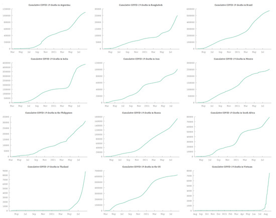
Figure 1. Cumulative deaths from COVID-19 for the 12 selected countries from 19 February 2020 to 20 August 2021. Source: Our World in Data (2021).

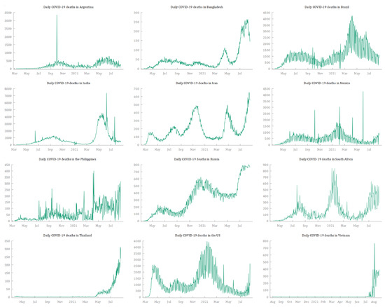
Figure 2. Daily deaths from COVID-19 for the 12 selected countries from 19 February 2020 to 20 August 2021. Source: Our World in Data (2021).

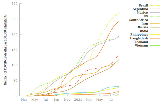
Figure 3. The number of deaths from COVID-19 per 100,000 inhabitants in 12 hard-hit big countries from 19 February 2020 to 20 August 2021. Source: Author’s elaborations on Source: Our World in Data (2021) and World Bank (2021).

4. Methodology

4.1. ARIMA and SARIMA Models

The non-seasonal ARIMA model is classified as “ARIMA(p,d,q)”, where: p is the order of the autoregressive (AR) process, d is the order of differencing required by the time series to get stationary, and q is the order of the moving average (MA) process. By multiplying the seasonal terms by the non-seasonal terms in the ARIMA model, it is possible to get a seasonal ARIMA (SARIMA) model. It assumes the notation “SARIMA (p,d,q)(P,D,Q)_m”, where: m is the frequency of data, and the lowercase and uppercase notations refer to the non-seasonal and seasonal components of the model, respectively.

The analysis used the following steps:

• First, I split the original dataset into training and test sets, and I ran the model with the training set. Its output was compared with the target, i.e., the test set. In particular, the training set was used to predict the last 20 observations of the original dataset.1 The best ARIMA and SARIMA2 models were identified using the “auto.arima( )” function included in the package “forecast” (in the R software), developed by Hyndman and Khandakar (2008).3 This function follows sequential steps to identify the best model to fit. It finds the best model by using the unit root test to assess the non-seasonal and seasonal degrees of difference necessary to make the time series stationary4 and by looking at the minimization of the Akaike’s information criterion (AIC) and the maximum likelihood estimation (MLE).5 This procedure was used to prevent issues of overfitting and underfitting and to evaluate the overall performance of the model, i.e., its ability to predict unseen data. In addition, as suggested by Hyndman and Athanasopoulos (2021, sct. 5.2), I also compared my preferred methods to three simple forecasting methods, i.e., Mean, Naïve, and Seasonal Naïve approaches.6 To assess the suitability of each model, I used the mean absolute percentage error (MAPE) metric. In fact, it is the most widely used error metric (Kim and Kim 2016; Hyndman and Athanasopoulos 2018, sct. 3.4), and it is not scale-dependent. Thus, it is easily comparable, immediately giving a good approximation of the accuracy of the models.7
• Second, I forecasted the time window of specific interest, from 21 August 2021 to 19 September 2021, and I compared the best ARIMA and SARIMA models on the minimization of AIC and four common measures of the accuracy of models: the mean absolute error (MAE), MAPE, mean absolute scaled error (MASE) and the root mean squared error (RMSE). After identifying the best models with the “auto.arima( )” function, I fitted the SARIMA models with Gretl-2021-c software, using the exact MLE approach and standard errors of parameters based on the Hessian matrix.
• Then, I investigated the autocorrelation function (ACF) and the partial autocorrelation function (PACF) of the residuals for the first 14 lags to establish if the residuals described a white noise process. If signs of autocorrelation were present, as suggested by Hyndman and Athanasopoulos (2018, sct. 8.7), I graphically investigated ACF and PACF of the original time series (after differencing), and I added enough parameters until the residuals showed to be randomly distributed. This iterative process was based on the minimization of AIC and four common measures of the accuracy of models: MAE, MAPE, MASE, and RMSE.8
• Finally, I compared 30-day forecasts, from 21 August 2021 to 19 September 2021, with the actual trends (real-time data) to assess the overall reliability of the models by looking at the MAPE between them.

The steps of this procedure are summarized in Figure 4. The estimated baseline equation for the ARIMA models with (p,d,q) non-seasonal order terms was the following (Davidson 2000)9:

$${\mathsf{\Delta }}_{y_t}^d={\varphi }_1{\mathsf{\Delta }}_{y_{t-1}}^d+\dots {\varphi }_p{\mathsf{\Delta }}_{y_{t-p}}^d+{\gamma }_1{\epsilon }_{t-1}+\dots {\gamma }_q{\epsilon }_{t-q}+{\epsilon }_t,$$

(1)

where ${\mathsf{\Delta }}^d$ is the difference operator,10 $y_t$ means the forecasted values, $p$ is the lag order of the AR process, $\varphi$ is the coefficient of each parameter $p$, $q$ is the order of the MA process, $\gamma$ is the coefficient of each parameter $q$, and ${\epsilon }_t$ denotes the residuals of the errors at time $t$.

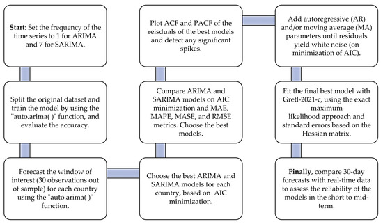
Figure 4. Nine sequential steps to identify and evaluate the best forecasting models for cumulative deaths from COVID-19.

The estimated basic equation for the SARIMA models with (p,d,q) non-seasonal order terms and (P,D,Q) seasonal order terms was the following (Chatfield 2000; Clarke and Clarke 2018):

$${\varphi }_P\left(B\right){\Phi }_P\left(B^s\right)(1-B){}^d(1-B^s){}^D{Y}_t={\theta }_q\left(B\right){\mathsf{\Theta }}_q\left(B^s\right){\epsilon }_t$$

(2)

where:

$${\varphi }_p\left(B\right)=(1-{\varphi }_{1}B-\dots -{\varphi }_p{B}^p)$$

(3)

$${\theta }_q\left(B\right)=(1-{\theta }_{1}B-\dots -{\theta }_q{B}^q)$$

(4)

$${\Phi }_P\left(B^s\right)=(1-{\Phi }_1{B}^s-\dots -{\Phi }_P{B}^{sP})$$

(5)

$${\mathsf{\Theta }}_Q\left(B^s\right)=(1-{\mathsf{\Theta }}_1{B}^s-\dots -{\mathsf{\Theta }}_Q{B}^{sQ})$$

(6)

where d is the order of non-seasonal differencing, D is the order of seasonal differencing, s is the number of seasons per year, $B$ is the backshift operator, ${\varphi }_p\left(B\right)$ and ${\theta }_q\left(B\right)$ denote the non-seasonal polynomials of order $p$ and $q$ in $B$, ${\Phi }_P\left(B^S\right)$ and ${\mathsf{\Theta }}_Q\left(B^S\right)$ denote the seasonal polynomials of order $P$ and $Q$ in $B^S$, and ${\epsilon }_t$ denotes the residuals of the errors at time $t$.

4.2. Evaluation Metrics

I used four common metrics—MAE, MAPE, MASE, and RMSE—to evaluate the overall accuracy of the forecasted models. In fact, since each of these error measures has specific characteristics and criticalities, I safely considered them jointly in the analysis (omitted reference). The formulae used to calculate each of these metrics were:

$$\mathrm{MAE}=\frac{1}{\mathrm{n}}{{\displaystyle \sum }}_{\mathrm{i}=1}^{\mathrm{n}}\left|y_i-{\widehat{\mathrm{y}}}_{\mathrm{i}}\right|$$

(7)

$$\mathrm{MAPE}=\frac{1}{\mathrm{n}}{\displaystyle \sum }_{\mathrm{i}=1}^{\mathrm{n}}\frac{\left|y_i-{\widehat{\mathrm{y}}}_{\mathrm{i}}\right|}{y_i}\ast 100\%$$

(8)

$$\mathrm{MASE}=\frac{1}{\mathrm{n}}{{\displaystyle \sum }}_{\mathrm{i}=1}^{\mathrm{n}}\left(\frac{\left|{\mathrm{y}}_{\mathrm{i}}-{\widehat{\mathrm{y}}}_{\mathrm{i}}\right|}{\frac{1}{\mathrm{n}-1}{{\displaystyle \sum }}_{\mathrm{i}=2}^{\mathrm{n}}\left|{\mathrm{y}}_{\mathrm{i}}-{\widehat{\mathrm{y}}}_{\mathrm{i}}-1\right|}\right)$$

(9)

$$\mathrm{RMSE}=\sqrt{\frac{1}{\mathrm{n}}{{\displaystyle \sum }}_{\mathrm{i}=1}^{\mathrm{n}}\left({\mathrm{y}}_{\mathrm{i}}-{\widehat{\mathrm{y}}}_{\mathrm{i}}\right)²}$$

(10)

where n represents the number of observations, ${\mathrm{y}}_{\mathrm{i}}$ denotes the actual values, and $\widehat{{\mathrm{y}}_{\mathrm{i}}}$ indicates the forecasted values.

5. Results and Discussion

Figure 5 and Figure 6 show the results of the training and test sets for each country by fitting ARIMA and SARIMA models, respectively. The training set and the test set exhibited, in most cases, very low and similar MAPE for ARIMA and SARIMA models. The only exception was the ARIMA model for Vietnam, where MAPE for the test set was 15 times larger than MAPE for the training set. In this case, MAPE for the test set was definitively greater than that for the training set, suggesting overfitting issues. However, this is not particularly worrying because the SARIMA model for Vietnam exhibited much better performance than the ARIMA model. Moreover, SARIMA outperformed both ARIMA models and the simple forecasting methods used as benchmarks, i.e., Mean, Naïve, and Seasonal Naïve (Table 3). Notably, MAPE for SARIMA models was always lower or very close to 1%, except for Vietnam. This could be deemed a satisfying output considering that many factors were not included in the forecasting process, such as climate and environmental conditions, the efficiency and capacity of the health systems, non-pharmaceutical interventions (lockdowns, physical distancing, quarantine), the age structure of the population, and vaccination campaigns.11 Thus, the models seem able to learn from previous data, and they can be effective in predicting unseen observations.

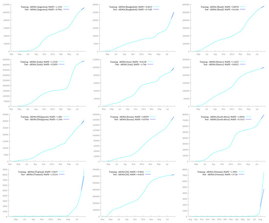
Figure 5. ARIMA forecasting models built on the training set over the period 1 August 2021–20 August 2021, in Argentina, Bangladesh, Brazil, India, Iran, Mexico, the Philippines, Russia, South Africa, Thailand, the US, and Vietnam.

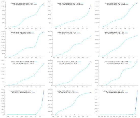
Figure 6. SARIMA forecasts on the training set over the period 1 August 2021–20 August 2021, in Argentina, Bangladesh, Brazil, India, Iran, Mexico, the Philippines, Russia, South Africa, Thailand, the US, and Vietnam.

Table 3. Comparing ARIMA and SARIMA approaches to three simple statistical methods (Mean, Naïve, and Seasonal Naïve).

Methods		AR	BD	BR	IN	IR	MX
Mean	Training	72,976.46	9848.56	77,102.94	165,478.16	15,028.63	80,758.69
	Test	65.428	71.1171	64.6042	68.3176	58.2728	53.0982
Naïve	Training	2.1205	1.8492	2.3508	2.4336	1.8627	2.285
	Test	2.1855	10.3307	1.5637	1.1819	5.0682	2.0799
Seasonal Naïve	Training	12.6593	10.3185	10.959	12.9676	9.0316	11.3767
	Test	3.1073	13.4784	2.1704	1.6031	6.0435	2.6464
ARIMA	Training	1.1251	0.8419	0.8078	1.1925	0.4128	1.1023
	Test	0.7961	0.7185	0.4104	0.2059	1.746	0.6032
SARIMA	Training	1.0683	0.8141	0.4796	1.1867	0.364	1.026
	Test	0.7081	0.4334	0.1098	0.6559	1.4504	0.5796
Methods		PH	RU	ZA	TH	US	VN
Mean	Training	4911.19	83,559.78	27,054.27	627.5129	173,294.91	92.761
	Test	68.9418	67.2429	61.9092	94.129	49.7039	98.1843
Naïve	Training	1.8171	2.1524	2.0984	1.5583	2.2007	1.5119
	Test	5.1284	4.8805	4.7421	25.8882	0.9331	60.9863
Seasonal Naïve	Training	9.4063	11.8052	11.6468	7.9684	9.8018	7.1452
	Test	6.5852	6.3732	6.3233	33.0028	1.1509	79.0645
ARIMA	Training	1.001	0.8599	1.0944	0.837	0.9601	1.7891
	Test	1.344	0.0784	0.1913	2.3214	0.4333	27.36
SARIMA	Training	0.9768	0.5512	0.7008	0.8679	0.606	1.5797
	Test	1.0353	0.0782	0.4488	0.2977	0.3122	7.98

Countries: AR, Argentina; BD, Bangladesh; BR, Brazil; IN, India; IR, Iran; MX, Mexico; PH, the Philippines; RU, Russia; ZA, South Africa; TH, Thailand; US, the United States; VN, Vietnam.

In Table 4, I present the ARIMA models for forecasting the cumulative deaths from COVID-19 for each country in the period from 21 August 2021 to 19 September 2021, chosen by using the “auto.arima( )” function. Adding the seasonal effect in the “auto.arima( )” algorithm, I attained the SARIMA models for each country. However, looking at the plots of the ACF and PACF for lags up to 14, it seems that there is structure left in the residuals of the SARIMA fitted models for Bangladesh, Brazil, Iran, the Philippines, Russia, South Africa, Thailand, the US, and Vietnam (Figure S1, in Supplementary Materials S1). Therefore, I adjusted model parameters until I attained a white noise process.12 The final optimal SARIMA models are reported in Table 5.13

Table 4. Forecast accuracy measures for ARIMA models performed on cumulative deaths from COVID-19.

Countries	Parameters	AIC	MAE	MAPE	MASE	RMSE
Argentina	(3,2,2)	6881.541	66.581	1.0787	0.3196	159.55
Bangladesh	(3,2,2)	3812.116	6.7566	0.8228	0.1378	9.3994
Brazil	(3,2,2)	7664.725	265.97	0.7199	0.2541	378.57
India	(0,2,1)	7655.07	126.01	1.152	0.1524	348.46
Iran	(1,2,4)	5023.525	16.479	0.4051	0.0893	23.59
Mexico	(2,2,2)	7508.783	190.91	1.0532	0.3924	336.16
Philippines	(4,2,1)	5489.394	26.527	0.9718	0.4464	44.104
Russia	(3,2,2)	5217.116	27.871	0.9781	0.0764	36.772
South Africa	(2,2,3)	5776.75	44.677	1.0602	0.288	68.688
Thailand	(1,2,4)	3760.553	3.2342	0.9101	0.188	9.255
US	(5,2,0)	7751.229	212.06	0.9297	0.181	325.17
Vietnam	(1,2,4)	3945.154	8.2099	1.9751	0.4174	40.251

Table 5. Forecast accuracy measures for SARIMA models performed on cumulative deaths from COVID-19.

Countries	Parameters	AIC	MAE	MAPE	MASE	RMSE
Argentina	(0,2,1)(2,0,2)7	6851.536	58.478	1.0298	0.0399	154.55
Bangladesh	(3,1,3)(1,1,2)7	3745.92	6.425	0.5554	0.0192	8.9982
Brazil	(1,1,8)(0,1,1)7	7190.918	162.06	0.4563	0.021	256.97
India	(0,2,1)(2,0,2)7	7652.34	126	1.1499	0.0216	344.51
Iran	(6,2,2)(2,0,1)7	4944.182	15.442	0.3413	0.0122	21.571
Mexico	(0,2,1)(4,0,0)7	7438.09	156.18	0.9417	0.0456	312.81
Philippines	(6,2,4)(3,0,4)7	5456.546	24.988	0.9385	0.9385	41.113
Russia	(4,2,4)(4,0,3)7	4826.443	17.983	0.6797	0.0079	24.422
South Africa	(5,1,8)(4,1,4)7	5665.571	41.036	0.6862	0.0373	62.244
Thailand	(4,2,10)(4,0,2)7	3536.975	2.8601	0.9368	0.0261	7.0336
US	(6,1,1)(0,1,1)7	7446.294	172.95	0.5977	0.0208	263.14
Vietnam	(5,2,4)(0,0,1)7	3903.771	7.8076	1.9188	0.0651	37.599

In Table 6, I compare the ARIMA and SARIMA models on the minimization of AIC and on common accuracy metrics (MAE, MAPE, MASE, and RMSE). The outcomes show that SARIMA models outperformed ARIMA models in 46 out 48 metrics, i.e., on 95.8% of all the forecast accuracy measures, except for MASE in the Philippines and MAPE in Thailand. Since AIC is always lower for SARIMA models, adding seasonal terms seems to be justified. Specifically, SARIMA models minimize AIC from 0.04% for India to 7.49% for Russia, MAE from 0.01% for India to 39.07% for Brazil, MAPE from 0.18% for India to 36.62% for Brazil, MASE from 84.4% for Vietnam to 91.74% for Brazil, and RMSE from 1.13% for India to 33.59% for Russia.

Table 6. Comparison between ARIMA and SARIMA models, considering the minimization of AIC, MAE, MAPE, MASE, and RMSE metrics (in percentage), for cumulative deaths from COVID-19.

Countries	AIC	MAE	MAPE	MASE	RMSE
Argentina	−0.44	−12.17	−4.53	−87.52	−3.13
Bangladesh	−1.74	−4.91	−32.5	−86.07	−4.27
Brazil	−6.18	−39.07	−36.62	−91.74	−32.12
India	−0.036	−0.008	−0.18	−85.83	−1.13
Iran	−1.58	−6.29	−15.75	−86.34	−8.56
Mexico	−0.94	−18.19	−10.59	−88.38	−6.95
Philippines	−0.598	−5.8	−3.43	110.24	−6.78
Russia	−7.49	−35.48	−30.51	−89.66	−33.59
South Africa	−1.92	−8.15	−35.28	−87.05	−9.38
Thailand	−5.95	−11.57	2.93	−86.12	−24
US	−3.93	−18.44	−35.71	−88.51	−19.08
Vietnam	−1.05	−4.9	−2.85	−84.4	−6.59

Notes: negative (positive) values show the percentage efficiency gain (loss) from using SARIMA models. Roman values indicate that SARIMA models were better, while italic values indicate that ARIMA models were better.

Therefore, the optimal number of parameters for predicting cumulative the deaths from COVID-19 for each country were the following (Table 5): Argentina (0,2,1)(2,0,2)₇, Bangladesh (3,1,3)(1,1,2)₇, Brazil (1,1,8)(0,1,1)₇, India (0,2,1)(2,0,2)₇, Iran (6,2,2)(2,0,1)₇, Mexico (0,2,1)(4,0,0)₇, the Philippines (6,2,4)(3,0,4)₇, Russia (4,2,4)(4,0,3)₇, South Africa (5,1,8)(4,1,4)₇, Thailand (4,2,10)(4,0,2)₇, the US (6,1,1)(0,1,1)₇, and Vietnam (5,2,4)(0,0,1)₇.

Since MASE was always much lower than 1, the actual forecast performance is much better than the naïve method (Table 5).14 In other words, the proposed method yields smaller errors than one-step errors from the average naïve method (Hyndman and Koehler 2006). According to Lewis (1982), the results of MAPE indicated that SARIMA models had very high accuracy. In fact, the MAPE difference between the observed and fitted data was much smaller than 10%, ranging from 0.34% for Iran to 1.92% for Vietnam. Notably, except for Argentina, India, and Vietnam, the remaining countries had a MAPE smaller than 1% (Table 5). The excellent goodness of fit is confirmed by the analysis of ACF and PACF of the models (Figure 7). In fact, both functions did not show any significant spike, suggesting that residuals were not correlated in all the countries analyzed. That is, the fitted data described a white noise process.

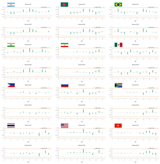
Figure 7. ACF and PACF plot of the residuals of the best SARIMA models (reported in Table 5).

In Figure 8 and Figure 9, I graphically represent the optimal SARIMA models for forecasting cumulative deaths from COVID-19 in the 12 hard-hit big countries in the next 30 days, from 21 August 2021 to 19 September 2021. The light blue area identifies the prediction interval at a 95% level of confidence. The red dashed line represents the forecasted values, and the light green continuous line identifies the original time series until 20 August 2021.

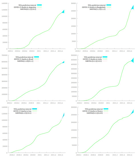
Figure 8. SARIMA models for forecasting the dynamics of cumulative deaths from COVID-19 over the period 21 August 2021–19 September 2021, in Argentina, Bangladesh, Brazil, India, Iran, and Mexico.

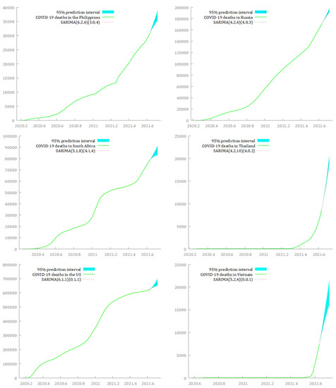
Figure 9. SARIMA models for forecasting the dynamics of cumulative deaths from COVID-19 over the period 21 August 2021–19 September 2021, in the Philippines, Russia, South Africa, Thailand, the US, and Vietnam.

Although the predictions seem to stress a common upward trend for cumulative deaths from COVID-19 in the next 30 days for all the countries, the fitted curves of the forecasted values exhibit different slopes. A slowdown in the growth curve of the deaths from COVID-19 seems to be possible in Argentina, Bangladesh, Brazil, and India. In this respect, the predicted values underline the likelihood of a flattening in the curves of cumulative deaths from COVID-19 around the end of September 2021. On the contrary, Iran, Mexico, the Philippines, South Africa, Russia, Thailand, the US, and Vietnam appear to be characterized by sustained growth of the total deaths from COVID-19 in the next 30 days. Among them, Thailand and Vietnam show a possible explosive growth in the number of deaths from COVID-19 in the same period.

Notably, Brazil, Iran, the Philippines, Russia, Thailand, and the US had the smallest prediction intervals, suggesting a low uncertainty in estimating deaths from COVID-19 at the 95% level of confidence, while Argentina, Bangladesh, India, and Vietnam had the largest prediction intervals.

Finally, in Figure 10 and Figure 11, I compare the estimated models to the real-time data over the period 21 August 2021 to 19 September 2021. The predictions from the SARIMA models seemed to fit very well with the observed data over that time window. The only exception was Thailand, whose forecasts—although also increasing—overestimated the real trend.15

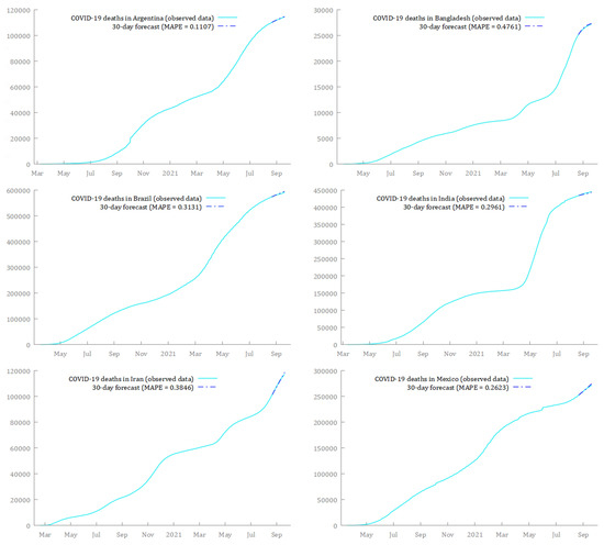
Figure 10. Comparison between forecasts and real data during the period 21 August 2021–19 September 2021, for cumulative deaths from COVID-19, in Argentina, Bangladesh, Brazil, India, Iran, and Mexico.

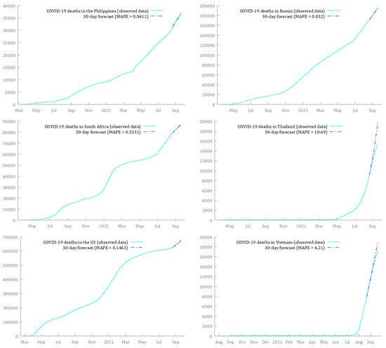
Figure 11. Comparison between forecasts and real data during the period 21 August 2021–19 September 2021, for cumulative deaths from COVID-19, in the Philippines, Russia, South Africa, Thailand, the US, and Vietnam.

Table 7 shows that MAPE difference between forecasted and observed data tended, on average, to grow in all countries. However, this is not particularly worrying because the absolute values of MAPE generally remained low over the whole forecasting window. On 19 September 2021 (i.e., after 30 days), MAPE was lower than 1% for ten out of twelve countries, that is, 83.33% of the sample (Table 7). The highest values were reached by Vietnam and Thailand, with a MAPE of 4.21% and 10.69%, respectively. Russia, Argentina, and the US showed the lowest MAPE after 30 days, with average differences between forecasted and observed data of 0.03%, 0.11%, and 0.15%, respectively. Thus, the models proved to be not only accurate but also reliable enough in short- to mid-term. This is consistent with the recent literature (Khan and Gupta 2020; Alabdulrazzaq et al. 2021; Al-Turaiki et al. 2021; ArunKumar et al. 2021) and suggests the suitability of the SARIMA models to predict the trend of cumulative deaths from COVID-19 around the world.

Table 7. Comparison of forecasted values and real-time data over the period 21 August 2021–19 September 2021, considering the MAPE difference between them.

Countries	Values	Values	Values	Values
	Until 25 August 2021	Until 30 August 2021	Until 9 September 2021	Until 19 September 2021
Argentina	0.057	0.061	0.09	0.1107
Bangladesh	0.1955	0.3179	0.4651	0.4761
Brazil	0.0271	0.0588	0.1691	0.3131
India	0.0479	0.1376	0.2671	0.2961
Iran	0.0981	0.2209	0.2975	0.3846
Mexico	0.0515	0.0642	0.0808	0.2623
Philippines	0.6835	0.6182	0.5423	0.8411
Russia	0.0076	0.011	0.014	0.032
South Africa	0.0558	0.092	0.132	0.3331
Thailand	1.2301	2.4151	5.6266	10.6897
US	0.0848	0.1124	0.1458	0.1463
Vietnam	1.2779	1.4391	2.6018	4.2089

6. Conclusions

In this paper, I attempted to forecast the cumulative deaths from COVID-19 in 12 hard-hit big countries for the period 21 August 2021–19 September 2021. The results showed that: (i) the implemented forecasting procedures proved to have a good prediction accuracy both in the training and the test set, by outperforming the simple alternative methods (Mean, Naïve, and Seasonal Naïve); (ii) SARIMA models outperformed ARIMA models (in predicting future values) on AIC and almost all the considered forecast accuracy measures (MAE, MAPE, MASE, and RMSE), suggesting the existence of strong seasonal patterns in the time series; and (iii) the 30-day forecasts from the SARIMA models fitted very well the observed data over the period 21 August 2021–19 September 2021 in almost all the countries analyzed.

Thus, SARIMA models were shown to be accurate and reliable tools for forecasting cumulative deaths from COVID-19. They adapted very well to the implemented data, even with complex patterns and seasonality. This is consistent with the extensive and successful use of this approach in the recent literature for predicting the outcomes of the COVID-19 disease (ArunKumar et al. 2021; Malki et al. 2021; Satpathy et al. 2021). Although predictions beyond 15 or 20 days should be taken with some caution, the models estimated in this article may give a reliable approximation of the pattern of growth of the main dimensions of the COVID-19 pandemic and other similar diseases. In particular, SARIMA models proved that they could be safely used for both the short- and mid-term. Therefore, these predictions can help the government authorities to monitor and manage the huge pressure that COVID-19 is exerting on national healthcare systems.

References

- Adebiyi, Ariyo A., Aderemi O. Adewumi, and Charles K. Ayo. 2014. Comparison of ARIMA and artificial neural networks models for stock price prediction. Journal of Applied Mathematics 2014: 614342. [Google Scholar] [CrossRef] [Green Version]
- Ahmad, Amir, Sunita Garhwal, Santosh K. Ray, Gagan Kumar, Sharaf J. Malebary, and Omar M. Barukab. 2021. The number of confirmed cases of covid-19 by using machine learning: Methods and challenges. Archives of Computational Methods in Engineering 28: 2645–53. [Google Scholar] [CrossRef] [PubMed]
- Ala’raj, Maher, Munir Majdalawieh, and Nishara Nizamuddin. 2021. Modeling and forecasting of COVID-19 using a hybrid dynamic model based on SEIRD with ARIMA corrections. Infectious Disease Modelling 6: 98–111. [Google Scholar] [CrossRef] [PubMed]
- Alabdulrazzaq, Haneen, Mohammed N. Alenezi, Yasmeen Rawajfih, Bareeq A. Alghannam, Abeer A. Al-Hassan, and Fawaz S. Al-Anzi. 2021. On the accuracy of ARIMA based prediction of COVID-19 spread. Results in Physics 27: 104509. [Google Scholar] [CrossRef]
- Al-Turaiki, Isra, Fahad Almutlaq, Hend Alrasheed, and Norah Alballa. 2021. Empirical evaluation of alternative time-series models for covid-19 forecasting in Saudi Arabia. International Journal of Environmental Research and Public Health 18: 8660. [Google Scholar] [CrossRef]
- Alzahrani, Saleh I., Ibrahim A. Aljamaan, and Ebrahim A. Al-Fakih. 2020. Forecasting the spread of the COVID-19 pandemic in Saudi Arabia using ARIMA prediction model under current public health interventions. Journal of Infection and Public Health 13: 914–19. [Google Scholar] [CrossRef]
- Annas, Suwardi, Muh I. Pratama, Muh Rifandi, Wahidah Sanusi, and Syafruddin Side. 2020. Stability analysis and numerical simulation of SEIR model for pandemic COVID-19 spread in Indonesia. Chaos, Solitons & Fractals 139: 110072. [Google Scholar]
- Ardabili, Sina F., Amir Mosavi, Pedram Ghamisi, Filip Ferdinand, Annamaria R. Varkonyi-Koczy, Uwe Reuter, Timon Rabczuk, and Peter M. Atkinson. 2020. Covid-19 outbreak prediction with machine learning. Algorithms 13: 249. [Google Scholar] [CrossRef]
- ArunKumar, K. E., Dinesh V. Kalaga, Ch. Mohan S. Kumar, Govinda Chilkoor, Masahiro Kawaji, and Timothy M. Brenza. 2021. Forecasting the dynamics of cumulative COVID-19 cases (confirmed, recovered and deaths) for top-16 countries using statistical machine learning models: Auto-Regressive Integrated Moving Average (ARIMA) and Seasonal Auto-Regressive Integrated Moving Average (SARIMA). Applied Soft Computing 103: 107161. [Google Scholar]
- Barnett, Adrian G., and Annette J. Dobson. 2010. Analysing Seasonal Health Data. Berlin: Springer. [Google Scholar]
- Box, George E. P., and George C. Tiao. 1975. Intervention analysis with applications to economic and environmental problems. Journal of the American Statistical Association 70: 70–79. [Google Scholar] [CrossRef]
- Box, George E. P., and Gwilym M. Jenkins. 1976. Time Series Analysis: Forecasting and Control. San Francisco: Holden-Day. [Google Scholar]
- Box, George E. P., Gwilym M. Jenkins, and Gregory C. Reinsel. 1994. Time Series Analysis: Forecasting and Control, 3rd ed. Prentice Hall: Englewood Cliff. [Google Scholar]
- Cao, Long-Ting, Hong-Hui Liu, Juan Li, Xiao-Dong Yin, Yu Duan, and Jing Wang. 2020. Relationship of meteorological factors and human brucellosis in Hebei province, China. Science of the Total Environment 703: 135491. [Google Scholar] [CrossRef] [PubMed]
- Carcione, José M., Juan E. Santos, Claudio Bagaini, and Jing Ba. 2020. A simulation of a COVID-19 epidemic based on a deterministic SEIR model. Frontiers in Public Health 8: 230. [Google Scholar] [CrossRef] [PubMed]
- Castillo Ossa, Luis F., Pablo Chamoso, Jeferson Arango-López, Francisco Pinto-Santos, Gustavo A. Isaza, Cristina Santa-Cruz-González, Alejandro Ceballos-Marquez, Guillermo Hernández, and Juan M. Corchado. 2021. A Hybrid Model for COVID-19 Monitoring and Prediction. Electronics 10: 799. [Google Scholar] [CrossRef]
- Centers for Disease Control and Prevention [CDC]. 2021. What You Need to Know about Variants. Updated on 6 August 2021. Available online: https://www.cdc.gov/coronavirus/2019-ncov/variants/variant.html (accessed on 23 August 2021).
- Ceylan, Zeynep. 2020. Estimation of COVID-19 prevalence in Italy, Spain, and France. Science of the Total Environment 729: 138817. [Google Scholar] [CrossRef] [PubMed]
- Chatfield, Chris. 2000. Time-Series Forecasting, 1st ed. Boca Raton: Chapman and Hall/CRC. [Google Scholar]
- Chintalapudi, Nalini, Gopi Battineni, and Francesco Amenta. 2020. COVID-19 virus outbreak forecasting of registered and recovered cases after sixty day lockdown in Italy: A data driven model approach. Journal of Microbiology, Immunology and Infection 53: 396–403. [Google Scholar] [CrossRef] [PubMed]
- Chung, Roy C., Andrew W. H. Ip, and Sian L. Chan. 2009. An ARIMA-intervention analysis model for the financial crisis in China’s manufacturing industry. International Journal of Engineering Business Management 1: 15–18. [Google Scholar] [CrossRef] [Green Version]
- Clarke, Bertrand S., and Jennifer L. Clarke. 2018. Predictive Statistics: Analysis and Inference Beyond Models. Cambridge: Cambridge University Press, vol. 46. [Google Scholar]
- Cong, Jing, Mengmeng Ren, Shuyang Xie, and Pingyu Wang. 2019. Predicting Seasonal Influenza Based on SARIMA Model, in Mainland China from 2005 to 2018. International Journal of Environmental Research and Public Health 16: 4760. [Google Scholar] [CrossRef] [PubMed] [Green Version]
- Conyon, Martin J., Lerong He, and Steen Thomsen. 2020. Lockdowns and COVID-19 Deaths in Scandinavia. Covid Economics 26: 17–42. [Google Scholar] [CrossRef]
- Davidson, James. 2000. Econometric Theory. Hoboken: Wiley Blackwell, p. 528. [Google Scholar]
- Dickey, David A., and Wayne A. Fuller. 1979. Distribution of the estimators for autoregressive time series with a unit root. Journal of the American Statistical Association 74: 427–31. [Google Scholar]
- Earnest, Arul, Mark I. Chen, Donald Ng, and Leo Y. Sin. 2005. Using autoregressive integrated moving average (ARIMA) models to predict and monitor the number of beds occupied during a SARS outbreak in a tertiary hospital in Singapore. BMC Health Services Research 5: 1–8. [Google Scholar] [CrossRef] [Green Version]
- Engbert, Ralf, Maximilian M. Rabe, Reinhold Kliegl, and Sebastian Reich. 2021. Sequential data assimilation of the stochastic SEIR epidemic model for regional COVID-19 dynamics. Bulletin of Mathematical Biology 83: 1–16. [Google Scholar] [CrossRef] [PubMed]
- Gaudart, Jean, Ousmane Touré, Nadine Dessay, lassane A. Dicko, Stéphane Ranque, Loic Forest, Jacques Demongeot, and Ogobara K. Doumbo. 2009. Modelling malaria incidence with environmental dependency in a locality of Sudanese savannah area, Mali. Malaria Journal 8: 1–12. [Google Scholar] [CrossRef] [PubMed]
- Hasan, Najmul. 2020. A methodological approach for predicting COVID-19 epidemic using EEMD-ANN hybrid model. Internet of Things 11: 100228. [Google Scholar] [CrossRef]
- He, Zhirui, and Hongbing Tao. 2018. Epidemiology and ARIMA model of positive-rate of influenza viruses among children in Wuhan, China: A nine-year retrospective study. International Journal of Infectious Diseases 74: 61–70. [Google Scholar] [CrossRef] [Green Version]
- Hossain, Mohammad S., Mahbubul H. Siddiqee, Umme R. Siddiqi, Enayetur Raheem, Rokeya Akter, and Wenbiao Hu. 2020. Dengue in a crowded megacity: Lessons learnt from 2019 outbreak in Dhaka, Bangladesh. PLoS Neglected Tropical Diseases 14: e0008349. [Google Scholar] [CrossRef]
- Hyndman, Rob J. 2013. 2013 Forecasting with Daily Data, 13 September 2013. Available online: https://robjhyndman.com/hyndsight/dailydata/ (accessed on 5 October 2021).
- Hyndman, Rob J. 2014. Unit Root Tests and ARIMA Models. 12 March 2014. Available online: https://robjhyndman.com/hyndsight/unit-root-tests/ (accessed on 5 October 2021).
- Hyndman, Rob J., and Yeasmin Khandakar. 2008. Automatic time series forecasting: The forecast package for R. Journal of Statistical Software 27: 1–22. [Google Scholar] [CrossRef] [Green Version]
- Hyndman, Rob J., and Anne B. Koehler. 2006. Another look at measures of forecast accuracy. International Journal of Forecasting 22: 679–88. [Google Scholar] [CrossRef] [Green Version]
- Hyndman, Rob J., and George Athanasopoulos. 2018. Forecasting: Principles and Practice, 2nd ed. Melbourne: Monash University, Available online: https://otexts.com/fpp2/ (accessed on 10 August 2021).
- Hyndman, Rob J., and George Athanasopoulos. 2021. Forecasting: Principles and Practice, 3rd ed. Melbourne: Monash University, Available online: https://otexts.com/fpp3/ (accessed on 12 March 2022).
- Kane, Michael J., Natalie Price, Matthew Scotch, and Peter Rabinowitz. 2014. Comparison of ARIMA and Random Forest time series models for prediction of avian influenza H5N1 outbreaks. BMC Bioinformatics 15: 276. [Google Scholar] [CrossRef]
- Katoch, Rupinder, and Arpit Sidhu. 2021. An Application of ARIMA Model to Forecast the Dynamics of COVID-19 Epidemic in India. Global Business Review. [Google Scholar] [CrossRef]
- Khan, Farhan M., and Rajiv Gupta. 2020. ARIMA and NAR based prediction model for time series analysis of COVID-19 cases in India. Journal of Safety Science and Resilience 1: 12–18. [Google Scholar] [CrossRef]
- Kim, Sungil, and Heeyoung Kim. 2016. A new metric of absolute percentage error for intermittent demand forecasts. International Journal of Forecasting 32: 669–79. [Google Scholar] [CrossRef]
- Korolev, Ivan. 2021. Identification and estimation of the SEIRD epidemic model for COVID-19. Journal of Econometrics 220: 63–85. [Google Scholar] [CrossRef] [PubMed]
- Kufel, Tadeusz. 2020. ARIMA-based forecasting of the dynamics of confirmed Covid-19 cases for selected European countries. Equilibrium. Quarterly Journal of Economics and Economic Policy 15: 181–204. [Google Scholar]
- Kwekha-Rashid, Ameer S., Heamn N. Abduljabbar, and Bilal Alhayani. 2021. Coronavirus disease (COVID-19) cases analysis using machine-learning applications. Applied Nanoscience, 1–13. [Google Scholar] [CrossRef]
- Kwiatkowski, Denis, Peter C. B. Phillips, Peter Schmidt, and Yongcheol Shin. 1992. Testing the null hypothesis of stationarity against the alternative of a unit root: How sure are we that economic time series have a unit root? Journal of Econometrics 54: 159–78. [Google Scholar] [CrossRef]
- Lewis, Colin D. 1982. Industrial and Business Forecasting Methods: A Practical Guide to Exponential Smoothing and Curve Fitting. Boston and London: Butterworth Scientific. [Google Scholar]
- Li, Jizhen, Yuhong Li, Ming Ye, Sanqiao Yao, Chongchong Yu, Lei Wang, Weidong Wu, and Yongbin Wang. 2021. Forecasting the Tuberculosis Incidence Using a Novel Ensemble Empirical Mode Decomposition-Based Data-Driven Hybrid Model in Tibet, China. Infection and Drug Resistance 14: 1941. [Google Scholar] [CrossRef]
- Li, Qi, Na-Na Guo, Zhan-Ying Han, Yan-Bo Zhang, Shun-Xiang Qi, Yong-Gang Xu, Ya-Mei Wei, Xu Han, and Ying-Ying Liu. 2012. Application of an autoregressive integrated moving average model for predicting the incidence of hemorrhagic fever with renal syndrome. The American Journal of Tropical Medicine and Hygiene 87: 364. [Google Scholar] [CrossRef]
- Liu, X., Z. Lin, and Z. Feng. 2021. Short-term offshore wind speed forecast by seasonal ARIMA-A comparison against GRU and LSTM. Energy 227: 120492. [Google Scholar] [CrossRef]
- Liu, Lei, R. S. Luan, F. Yin, X. P. Zhu, and Q. Lü. 2016. Predicting the incidence of hand, foot and mouth disease in Sichuan province, China using the ARIMA model. Epidemiology & Infection 144: 144–51. [Google Scholar]
- Liu, Qiyong, Xiaodong Liu, Baofa Jiang, and Weizhong Yang. 2011. Forecasting incidence of hemorrhagic fever with renal syndrome in China using ARIMA model. BMC Infectious Diseases 11: 218. [Google Scholar] [CrossRef] [Green Version]
- Malki, Zohair, El-Sayed Atlam, Ashraf Ewis, Guesh Dagnew, Ahmad R. Alzighaibi, Ghada ELmarhomy, Mostafa A. Elhosseini, Aboul E. Hassanien, and Ibrahim Gad. 2021. ARIMA models for predicting the end of COVID-19 pandemic and the risk of second rebound. Neural Computing and Applications 33: 2929–48. [Google Scholar] [CrossRef] [PubMed]
- McCleary, Richard, Richard A. Hay, Errol E. Meidinger, and David McDowall. 1980. Applied Time Series Analysis for the Social Sciences. Beverly Hills: Sage Publications. [Google Scholar]
- Our World in Data. 2021. Our World in Data COVID-19 Dataset. Available online: https://ourworldindata.org/coronavirus (accessed on 25 September 2021).
- Pack, David J. 1990. In defense of ARIMA modeling. International Journal of Forecasting 6: 211–18. [Google Scholar] [CrossRef]
- Perone, Gaetano. 2020. An ARIMA Model to Forecast the Spread and the Final Size of COVID-2019 Epidemic in Italy. No. 20/07. HEDG-Health Econometrics and Data Group Working Paper Series. York: University of York. [Google Scholar]
- Perone, Gaetano. 2021a. The determinants of COVID-19 case fatality rate (CFR) in the Italian regions and provinces: An analysis of environmental, demographic, and healthcare factors. Science of the Total Environment 755: 142523. [Google Scholar] [CrossRef]
- Perone, Gaetano. 2021b. Comparison of ARIMA, ETS, NNAR, TBATS and hybrid models to forecast the second wave of COVID-19 hospitalizations in Italy. The European Journal of Health Economics, 1–24. [Google Scholar] [CrossRef]
- Phillips, Peter C., and Pierre Perron. 1988. Testing for a unit root in time series regression. Biometrika 75: 335–46. [Google Scholar] [CrossRef]
- Pinter, Gergo, Imre Felde, Amir Mosavi, Pedram Ghamisi, and Richard Gloaguen. 2020. COVID-19 pandemic prediction for Hungary; a hybrid machine learning approach. Mathematics 8: 890. [Google Scholar] [CrossRef]
- Piovella, Nicola. 2020. Analytical solution of SEIR model describing the free spread of the COVID-19 pandemic. Chaos, Solitons & Fractals 140: 110243. [Google Scholar] [CrossRef]
- Polwiang, Sittisede. 2020. The time series seasonal patterns of dengue fever and associated weather variables in Bangkok (2003–2017). BMC Infectious Diseases 20: 1–10. [Google Scholar] [CrossRef] [Green Version]
- Qiu, Hongfang, Han Zhao, Haiyan Xiang, Rong Ou, Jing Yi, Ling Hu, Hua Zhu, and Mengliang Ye. 2021. Forecasting the incidence of mumps in Chongqing based on a SARIMA model. BMC Public Health 21: 1–12. [Google Scholar] [CrossRef]
- Ren, Hong, Jian Li, Zheng-An Yuan, Jia-Yu Hu, Yan Yu, and Yi-Han Lu. 2013. The development of a combined mathematical model to forecast the incidence of hepatitis E in Shanghai, China. BMC Infectious Diseases 13: 421. [Google Scholar] [CrossRef] [Green Version]
- Roy, Santanu, Gouri S. Bhunia, and Pravat K. Shit. 2021. Spatial prediction of COVID-19 epidemic using ARIMA techniques in India. Modeling Earth Systems and Environment 7: 1385–91. [Google Scholar] [CrossRef] [PubMed]
- Safi, Samir K., and Olajide I. Sanusi. 2021. A hybrid of artificial neural network, exponential smoothing, and ARIMA models for COVID-19 time series forecasting. Model Assisted Statistics and Applications 16: 25–35. [Google Scholar] [CrossRef]
- Sahai, Alok K., Namita Rath, Vishal Sood, and Manvendra P. Singh. 2020. ARIMA modelling & forecasting of COVID-19 in top five affected countries. Diabetes & Metabolic Syndrome: Clinical Research & Reviews 14: 1419–27. [Google Scholar]
- Sarkodie, Samuel A., and Phebe A. Owusu. 2020. Impact of meteorological factors on COVID-19 pandemic: Evidence from top 20 countries with confirmed cases. Environmental Research 191: 110101. [Google Scholar] [CrossRef]
- Satpathy, Suneeta, Monika Mangla, Nonita Sharma, Hardik Deshmukh, and Sachinandan Mohanty. 2021. Predicting mortality rate and associated risks in COVID-19 patients. Spatial Information Research 29: 455–464. [Google Scholar] [CrossRef]
- Satrio, Christophorus. B. A., William Darmawan, Bellatasya U. Nadia, and Novita Hanafiah. 2021. Time series analysis and forecasting of coronavirus disease in Indonesia using ARIMA model and PROPHET. Procedia Computer Science 179: 524–32. [Google Scholar] [CrossRef]
- Sen, Parag, Mousumi Roy, and Parimal Pal. 2016. Application of ARIMA for forecasting energy consumption and GHG emission: A case study of an Indian pig iron manufacturing organization. Energy 116: 1031–38. [Google Scholar] [CrossRef]
- Singh, Sarbjit, Kulwinder S. Parmar, Jatinder Kumar, and Sidhu J. S. Makkhan. 2020. Development of new hybrid model of discrete wavelet decomposition and autoregressive integrated moving average (ARIMA) models in application to one month forecast the casualties cases of COVID-19. Chaos, Solitons & Fractals 135: 109866. [Google Scholar]
- Sujatha, R., Jyotir M. Chatterjee, and Aboul E. Hassanien. 2020. A machine learning forecasting model for COVID-19 pandemic in India. Stochastic Environmental Research and Risk Assessment 34: 959–72. [Google Scholar] [CrossRef]
- Talkhi, Nasrin, Narges A. Fatemi, Zahra Ataei, and Mehdi J. Nooghabi. 2021. Modeling and forecasting number of confirmed and death caused COVID-19 in IRAN: A comparison of time series forecasting methods. Biomedical Signal Processing and Control 66: 102494. [Google Scholar] [CrossRef]
- Tuli, Shreshth, Shikhar Tuli, Rakesh Tuli, and Sukhpal S. Gill. 2020. Predicting the growth and trend of COVID-19 pandemic using machine learning and cloud computing. Internet of Things 11: 100222. [Google Scholar] [CrossRef]
- Tran, Thai T., Thanh-Luu Pham, and Ngo X. Quang. 2020. Forecasting epidemic spread of SARS-CoV-2 using ARIMA model (Case study: Iran). Global Journal of Environmental Science and Management 6: 1–10. [Google Scholar]
- Valipour, Mohammad. 2015. Long-term runoff study using SARIMA and ARIMA models in the United States. Meteorological Applications 22: 592–98. [Google Scholar] [CrossRef]
- Viguerie, Alex, Guillermo Lorenzo, Ferdinando Auricchio, Davide Baroli, Thomas J. Hughes, Alessia Patton, Alessandro Reali, Thomas E. Yankeelov, and Alessandro Veneziani. 2021. Simulating the spread of COVID-19 via a spatially-resolved susceptible–exposed–infected–recovered–deceased (SEIRD) model with heterogeneous diffusion. Applied Mathematics Letters 111: 106617. [Google Scholar] [CrossRef]
- Wang, Lulu, Chen Liang, Wei Wu, Shengwen Wu, Jinghua Yang, Xiaobo Lu, Yuan Cai, and Cuihong Jin. 2019. Epidemic Situation of Brucellosis in Jinzhou City of China and Prediction Using the ARIMA Model. Canadian Journal of Infectious Diseases and Medical Microbiology 2019: 1429462. [Google Scholar] [CrossRef] [Green Version]
- Wang, Peipei, Xinqi Zheng, Jiayang Li, and Bangren Zhu. 2020. Prediction of epidemic trends in COVID-19 with logistic model and machine learning technics. Chaos, Solitons & Fractals 139: 110058. [Google Scholar]
- Wang, Xiaozhe, Kate A. Smith, and Rob J. Hyndman. 2006. Characteristic-based clustering for time series data. Data Mining and Knowledge Discovery 13: 335–64. [Google Scholar] [CrossRef]
- Wang, Ya-Wen, Zhong-Zhou Shen, and Yu Jiang. 2018. Comparison of ARIMA and GM (1, 1) models for prediction of hepatitis B in China. PLoS ONE 13: e0201987. [Google Scholar] [CrossRef]
- Wei, Wudi, Junjun Jiang, Hao Liang, Lian Gao, Bingyu Liang, Jiegang Huang, Ning Zang, Yanyan Liao, Jun Yu, Jingzhen Lai, and et al. 2016. Application of a Combined Model with Autoregressive Integrated Moving Average (ARIMA) and Generalized Regression Neural Network (GRNN) in Forecasting Hepatitis Incidence in Heng County, China. PLoS ONE 11: e0156768. [Google Scholar] [CrossRef]
- World Bank. 2021. World Bank Open Data. Available online: https://data.worldbank.org (accessed on 30 August 2021).
- Worldometer. 2021. Available online: https://www.worldometers.info/coronavirus/ (accessed on 30 August 2021).
- Xu, Qinqin, Runzi Li, Yafei Liu, Cheng Luo, Aiqiang Xu, Fuzhong Xue, Qing Xu, and Xiujun Li. 2017. Forecasting the incidence of mumps in Zibo City based on a SARIMA model. International Journal of Environmental Research and Public Health 14: 925. [Google Scholar] [CrossRef] [Green Version]
- Yousaf, Muhammad, Samiha Zahir, Muhammad Riaz, Sardar M. Hussain, and Kamal Shah. 2020. Statistical analysis of forecasting COVID-19 for upcoming month in Pakistan. Chaos, Solitons & Fractals 138: 109926. [Google Scholar]
- Zeng, Qianglin, Dandan Li, Gui Huang, Jin Xia, Xiaoming Wang, Yamei Zhang, Wanping Tang, and Hui Zhou. 2016. Time series analysis of temporal trends in the pertussis incidence in Mainland China from 2005 to 2016. Scientific Reports 6: 1–8. [Google Scholar] [CrossRef] [PubMed]
- Zhang, Lanyi, Jane Lin, Rongzu Qiu, Xisheng Hu, Huihui Zhang, Qingyao Chen, Huamei Tan, Danting Lin, and Jiankai Wang. 2018. Trend analysis and forecast of PM2. 5 in Fuzhou, China using the ARIMA model. Ecological Indicators 95: 702–10. [Google Scholar] [CrossRef]
- Zheng, Nanning, Shaoyi Du, Jianji Wang, He Zhang, Wenting Cui, Zijian Kang, Tao Yang, Bin Lou, Yuting Chi, Hong Long, and et al. 2020. Predicting COVID-19 in China using hybrid AI model. IEEE Transactions on Cybernetics 50: 2891–904. [Google Scholar] [CrossRef]
- Zheng, Yan-Ling, Li-Ping Zhang, Xue-Liang Zhang, Kai Wang, and Yu-Jian Zheng. 2015. Forecast model analysis for the morbidity of tuberculosis in Xinjiang, China. PLoS ONE 10: e0116832. [Google Scholar] [CrossRef]
Publisher’s Note: MDPI stays neutral with regard to jurisdictional claims in published maps and institutional affiliations. |
© 2022 by the author. Licensee MDPI, Basel, Switzerland. This article is an open access article distributed under the terms and conditions of the Creative Commons Attribution (CC BY) license (https://creativecommons.org/licenses/by/4.0/).