Abstract
The relationships between environmental characteristics and species richness in the grasslands of the Colombian Orinoquia are presented and analyzed using an ordinal logistic regression model. Ordinal and scale covariates were included, and their bivariate significance was assessed using Spearman’s rho and Kendall’s Tau-b. The covariates that showed statistical significance with the weighted richness thresholds (WRT) and defined the model were the soil depth and the soil moisture regime, both of which had positive correlations. In contrast, the percentage of bare soil and the monthly minimum temperature showed negative correlations. This contribution highlights the relevance of articulating and combining the floristic and phytosociological characterization of grassland vegetation to advance the predictive studies aimed at defining and understanding the potential divergent relationships between the vegetation and the basic attributes of the natural environment, along with their implications for conservation.
1. Introduction
The Neotropical savannas cover an area of approximately 2.5 million hectares. South of the Amazon, they include regions such as Beni (Bolivia), Cerrado (Brazil), and the Chaco (Paraguay); to the north lies the Orinoquia region, shared by Colombia and Venezuela [1,2,3,4,5]. Their ecological attributes are far from being extensively homogeneous, as there are clear geological, geomorphological, hydrological, climatic, topographic, and edaphic singularities that contribute to a biotic complexity of high conservation value [6,7,8,9,10,11,12,13,14].
Among the key contributions on the influence of habitat-defining factors on the richness and diversity of their plant communities is that of Bourlière and Hadley [15], who established relationships between vegetation structure and soil moisture, concluding that soil nutrients are a subordinate factor to climatic seasonality. Additionally, Sarmiento [16] documented the relationships between climatic seasonality, topography, and moisture regimes.
In the Brazilian cerrado, Goodland [17], Goodland and Pollard [18] and Lopes and Cox [19] documented the relationships between soil fertility gradients, leaf consistency, and the floristic composition of plant communities. They concluded that soil fertility is a decisive factor in explaining variations in species richness and floristic composition in these savannas. Pereira et al. [20] assessed the relationships between soil properties, species density, and species richness in savanna formations, concluding that soil characteristics (fertility, texture, and moisture) determine the geographic extent of vegetation formations, species abundance, and physiognomy. Menegat et al. [21] concluded that local edaphic and climatic variations, even within geographically proximate areas, significantly influence species richness and turnover in continuous vegetation formations. In the Beni savannas of Bolivia, Haase [22,23] concluded that precipitation regimes, soil moisture, and texture are the primary determinants of variations in species richness, structure, and floristic composition. Medina and Motta [24] identified the hydric gradient as the main factor explaining species richness and floristic composition. Van Donselaar [2] considered soil texture and moisture to be the most significant determinants of species richness and floristic composition in the Surinamese savannas. In the Venezuelan savannas, according to Sarmiento and Monasterio [25], geomorphology, parent material, soil depth, and drainage conditions showed the highest correlation with vegetation richness and diversity. Frost et al. [26] concluded that soil moisture and nutrient availability are the key factors in explaining species richness and floristic composition, with human activities identified as external modifying agents. Sarmiento and Pinillos [27] and Sarmiento et al. [28] established the relationship between geomorphology and hydrology with species richness and floristic composition. According to Chacón-Moreno et al. [29], soil fertility is not a determining factor, but water dynamics and water retention capacity are the principal determinants of species richness and distribution. Baruch [9] attributed the highest correlation with species richness to moisture and fertility indices, establishing that precipitation amounts and distribution, nutrient availability, and edaphic factors are the environmental determinants most influential in species richness, physiognomy, and levels of association in seasonal savannas.
Regarding the species richness and floristic composition of the Colombian Orinoquian grasslands, data indicate the presence of approximately 4800 species (Rangel-Ch. et al., in prep.). The phytosociological characterization encompasses one (1) class, three (3) orders, nineteen (19) alliances, and sixty-three (63) associations. In the high plains, the associations are composed, on average, of twenty-eight (28) characteristic/differential species, with notable contrasts in richness values, such as Desmodio barbati-Sipanetum pratensis (49 species) and Panico pilosi-Schizachyrietum brevifoli (13 spp.). In the alluvial plains, associations consist of an average of 38 species, with Ludwigio erectae-Axonopodetum purpusi (64 spp.) and Axonopodo ancepitis-Curatelletum americanae (22 spp.) standing out [5,30,31,32].
In contrast, the relationships between species richness expression in these vegetation types and the basic attributes of the natural environment have been scarcely addressed at the local scale and even less at the regional level. Beard [33] highlighted the influence of nutrient availability on species richness and structure. Other studies [1,32,34,35,36,37,38,39,40,41,42,43,44,45,46,47,48] provide a partial overview of the influence of edaphic conditions, flooding, and waterlogging on richness and diversity values.
Despite prior studies, there is no consensus regarding which set of ecological factors holds the greatest relevance for the floristic richness of the Colombian Orinoquian grasslands. The role of climatic and edaphic factors in shaping floristic richness and composition remains unclear. It is proposed that species richness in the grasslands of the Orinoco region is significantly influenced by climatic and edaphic factors. Specifically, temperature, precipitation, and soil characteristics such as texture, moisture, and aluminum content interact to shape species richness. Variations in these factors are expected to explain patterns of distribution and richness, demonstrating that certain combinations of climatic and edaphic conditions promote greater biodiversity expression in grasslands.
Therefore, it is necessary to conduct a more in-depth analysis of these factors to understand their impact on the floristic significance of the region. Thus, the primary objective of this manuscript is to propose a model for the phytocoenoses described in the Colombian Llanos, with the goal of addressing: (i) which set of ecological factors is most relevant to their floristic richness? and (ii) how do these attributes interact, and what is their influence on species richness values?
To address these questions, this study proposes the following hypothesis based on the 292 vegetation plots in the Colombian Orinoquian grasslands: climate and soil factors are the primary environmental attributes, and play different roles in shaping their floristic composition. These models are essential for deepening the understanding of the region, as they allow for a detailed description of its environmental and biotic singularities. Furthermore, they provide key inputs for the development of thematic maps and delineation of strategic (ecogeographic or biogeographic) areas for biodiversity conservation, such as national parks and newly protected areas, among others.
2. Results
Table 1 shows the frequencies of the dependent variable, corresponding to the weighted richness category, those considered as factors (nominal variables), and covariates (ordinal variables with their respective ordinal numerical reclassification). Table 2 presents the descriptive statistics of the scale covariates.

Table 1.
Frequencies of nominal and ordinal variables considered in the Colombian Orinoquian grassland’s floristic richness analysis.
Table 2.
Descriptive statistics of the ecological scalar variables in the Colombian Orinoquian grassland’s floristic richness analysis.
According to the bivariate exploratory analysis, the statistically significant covariates exhibited an inverse correlation with the weighted richness, with the exception of soil depth. Based on the magnitude of the statistically significant correlations, the percentage of bare soil showed the highest correlation with weighted richness, followed by minimum monthly precipitation, minimum monthly temperature, soil depth, maximum monthly temperature, annual mean precipitation, and soil moisture regime, respectively (Table 3).
Table 3.
Statistics from the ecological bivariate exploratory analysis in the Colombian Orinoquian grassland’s floristic richness.
In the bivariate Wald statistics, all values, except for minimum monthly temperature, were greater than two, indicating statistical significance; these results align with the significant associations in Table 3. Regarding VIF analysis, annual mean temperature and maximum monthly precipitation were removed due to their strong collinearity with maximum monthly temperature and annual mean precipitation, respectively. These exclusions ensured that the retained variables provided unique and independent contributions to the model, minimizing redundancy. By addressing multicollinearity, this step also improved the precision of estimated coefficients and the overall reliability of the ordinal regression models, enabling a clearer understanding of how climatic and edaphic factors are related to species richness. In the multivariate model, three of the Wald values are not significant, implying that in both the bivariate and multivariate exploratory analyses, the covariates of maximum monthly temperature, minimum monthly temperature, and annual mean precipitation do not contribute to the regression. Therefore, these variables should be eliminated to achieve a more parsimonious model. According to the error values, the variables with significant Wald statistics show disparate coefficients in the multivariate model compared to the bivariate model. This suggests that the relationship of these variables with weighted richness is affected by an interaction or confounding effect, as the statistical results depend on the inclusion or exclusion of other variables from the model (Table 4).
Table 4.
Comparison of bivariate and multivariate exploratory regression in the Colombian Orinoquian grassland’s floristic richness analysis.
The initial and final model fits, represented by the values of −2 log-likelihood (−2LL) and a Chi-square test on their difference (statistic = 38.795; significance = 0.000), indicating that the regression provides a significant improvement with the variables included in the final model (−2LL = 523.243) compared to the baseline or intercept model with only the constant (−2LL = 562.037).
The Cox and Snell R2 for the ordinal regression was calculated at 0.129, suggesting that 12.9% of the variation in weighted richness is attributed to the included covariates. The Nagelkerke R2 represents a scale adjustment of the Cox and Snell R2. The calculated value for the ordinal regression was 0.143, estimating that 14.3% of the variation in the dependent variable can be explained by the predictor variables. Although the pseudo R2 values were modest, these statistics are indicative between similar models but not conclusive, as none of them explain variance analogously to the R2 coefficient of linear regressions. The multicollinearity test indicated that the assumption of equal coefficients for all response categories is not rejected, thereby validating the feasibility of the ordinal procedure.
Table 5 shows the parameter estimates that summarize the effects of each predictor included in the grassland analysis. The statistical significance (<0.05) of the covariates related to soil depth, percentage of bare soil, and minimum monthly temperature suggest that the effect observed on weighted richness is not attributable to chance. Conversely, the significance of the soil depth covariate contributes little to the model, although it is close to the established cutoff point; this could be considered a marginally significant variable and may warrant retention in the regression, as the effects of covariates are cumulative and provide useful information.
Table 5.
Statistics from the ordinal regression for weighted richness in the Colombian Orinoquian grassland’s floristic richness.
According to the regression slope coefficients, both the soil depth and the soil moisture regime exhibit positive values, indicating that as their magnitudes increase, the probability of being classified in a higher category of weighted richness also increases; in other words, greater depth and moisture levels are associated with a higher number of species. Conversely, the percentage of bare soil and the minimum monthly temperature show negative coefficients, suggesting that an increase in their magnitudes corresponds to a higher probability of being classified in a lower category of weighted richness; thus, a greater proportion of bare soil and a higher temperature during the hottest month are associated with a lower number of species.
The model estimates the cumulative probabilities for each category of weighted richness, which are utilized in selecting the most probable outcome for each case. The calculation of these probabilities is performed using the predictor values in the model equations and the inverse of the link function, defined as the negative log-log based on the definitions of the variables. The probabilities for the individual categories of weighted richness can be estimated by sequentially taking the differences of the cumulative probabilities; specifically, the probability for the first category corresponds to the first cumulative probability, the probability for the second category is derived by subtracting the first cumulative probability from the second, and so on.
In line with the above, and utilizing the parameters from the ordinal regression, it is feasible to establish the model equations, which facilitate the calculation of the probability of belonging to each of the four categories of weighted richness, based on the link function (negative log-log) and the three thresholds (Table 5), which are defined below.
Model
- WRT = 1:
−log(−log(WRT1)) = 0.333 − (SOIL_DEPTH*0.311) − (SOIL_MOIST*0.154) − (BARE_SOIL*−0.027) − (MIN_MONTH_TEMP* − 0.067).
- WRT = 2:
−log(−log(WRT2)) = 1.599 − (SOIL_DEPTH*0.311) − (SOIL_MOIST*0.154) − (BARE_SOIL*−0.027) − (MIN_MONTH_TEMP* − 0.067).
- WRT = 3:
−log(−log(WRT3)) = 4.297 − (SOIL_DEPTH*0.311) − (SOIL_MOIST*0.154) − (BARE_SOIL*−0.027) − (MIN_MONTH_TEMP* − 0.067).
3. Discussion
3.1. Importance of Predictive Richness Models
The floristic composition and species richness of grassland communities are governed by many ecological drivers such as climate, soil moisture, humidity, and nutrient availability [49]. The relationships among these processes, environmental factors, and biocenoses have been extensively examined through various ecological models, emphasizing that the variation within phytocenoses is a direct response to local singularities and subsequently to regional heterogeneity (see, among others, [49,50,51,52,53,54,55]). Predictive richness models applied in ecology and vegetation science primarily focus on resolving how the fundamental attributes of the natural environment are differentially and asymmetrically combined in ostensibly homogeneous areas. Additionally, these models aim at clarifying the set of processes that define the richness and diversity of plant communities. In the case of grasslands (primarily Asian and European), their applications are multiscale and widely utilized in studies concerning species distribution patterns, population and community ecology, ecological niche characterization, flora and vegetation mapping, carbon capture, functional ecology, among others [49,50,55,56,57,58,59,60,61,62,63].
The model proposed herein estimates the probability and addresses questions regarding the primary factors affecting the expression of floristic richness in Colombian Orinoco grasslands. This opens up possibilities for advancing predictive studies aimed at defining and understanding potential divergent relationships (positive, negative, or incipient) between vegetation (zonal, azonal, or extrazonal) and the fundamental attributes of the natural environment. According to the bivariate exploratory analysis, the covariables that exhibited statistical significance concerning the thresholds of weighted richness (WRT) were soil depth, soil moisture regime, percentage of bare soil, minimum monthly temperature, maximum monthly temperature, mean annual precipitation, and minimum monthly precipitation. In the statistical contrast of the bivariate and multivariate regressions, the covariables of minimum monthly temperature, maximum monthly temperature, and mean annual precipitation were excluded. In the ordinal regression, the covariables defining the richness model were soil depth and soil moisture regime, both of which showed positive correlations. Conversely, the percentage of bare soil and minimum monthly temperature demonstrated negative correlations.
Our analysis reveals that environmental characteristics, particularly soil conditions and climatic variables, significantly impact the species richness of the studied grasslands. Specifically, a higher percentage of bare soil and elevated minimum monthly temperature are associated with lower species richness, suggesting that these factors limit plant diversity. On the other hand, greater soil depth correlates positively with species richness, indicating that deeper soils provide more favorable conditions for the establishment and development of a larger number of species. Furthermore, this model allows for an understanding of how these factors interact in accordance with the ecological particularities that define the physiographic units of the region, and what their effects are on the richness values, floristic composition and ecogeographical extent of its phytocenoses.
3.2. Ecological Aspects
Climate serves as the primary ecological filter at the regional scale, while variations in soil composition represent a more specific filter operating at the local level. This binomial influences richness, floristic composition, vegetation structure, and the autoecology of its species. Seasonality, precipitation amounts, and their distribution impact edaphic conditions (texture, fertility, pH). Water runoff consolidates substrates of variable nature (deficiency or excess of water), forming physiological barriers [64,65]. These aspects have been discussed, among others [66,67,68,69], where precipitation over other environmental factors was emphasized as the principal element defining the physiognomy, structure, and expression of richness in savanna formations.
The model proposed herein aligns with the findings of Peng et al. [70] and Qian et al. [71], which underscore how monthly fluctuations in precipitation amounts, soil composition, and topographical characteristics are closely related to geographical variations in vegetation types and, subsequently, their richness. It also corresponds with the considerations of Toledo et al. [72], who detail how the richness of grasslands is affected in the following order: precipitation > temperature > soil fertility > soil texture. Additionally, it partially conforms to the contributions of Sarmiento [73,74], Hasse [22,23], Solbrig et al. [75], and Anadon et al. [76], who highlight the relationships among topography, soil texture, moisture, water retention capacity, nutrients, climate, and their impact on the expression and significance of richness in neotropical savannas.
When stochastic scenarios prevail, floristic composition, richness, and the structure of plant communities exhibit considerable variability [54,77,78]. Numerous studies assess the combined effects of climatic and hydric variations alongside anthropogenic disturbances, as well as their applications for delineating conservation areas [79,80]. Models serve as predictive alternatives regarding how biota differentially interacts according to the fundamental attributes of the natural environment; however, it is crucial to emphasize the importance of recognizing and delving into the highly complex temporal effects, stress agents, and intrinsic dynamics of natural systems, which significantly impact their interpretation [49,80,81,82].
4. Materials and Methods
4.1. Study Area
The Colombian Orinoquia spans areas within the departments of Arauca, Casanare, Meta, and Vichada, covering approximately 17 million hectares (ca. 30% of the national territory), with elevations ranging between 180 and 675 m above sea level, featuring a slight slope towards the Northeast [38,44,83,84]. The tectonic conditions that led to its formation are associated with the rise of the Eastern Cordillera during the mid-Tertiary (Oligocene-Miocene) in two main fronts: a longer one between the Duda and Upía rivers, and a shorter, yet equally intense one in the El Cocuy region, along with continuous sedimentation through a river system that descended from the new mountainous system [35,85].
This region originated from a large geosyncline of alluvial sedimentary origin, influenced by tectonic events, Quaternary climate, ancient erosive processes in the Guiana Shield, and recent erosion from the Andes [86,87,88,89,90]. Although topographic contrasts are minimal, a complex mosaic of soils and micro-reliefs prevails, resulting from differential processes in the origin, age of the parent material, sedimentation, and land dissection [83]. Despite being recognized as a relatively homogeneous territory, with gentle slopes and predominantly covered by grasses [91], its physiography is closely related to chronological criteria, the distance from the Eastern Cordillera, and the Meta River, which demarcates drainage conditions influencing the relief variations: the poorly drained Orinoquia to the north of the river, characterized by fans and alluvial and aeolian plains, and the well-drained Orinoquia to the south, featuring predominantly flat and undulating high plains, hills, and terraces [1,34,41,44]. The sedimentary materials, both from the Tertiary and Quaternary periods, were deposited on an ancient platform belonging to the Guiana Shield, composed of Precambrian rocks aged between 1 and 1.8 billion years, with outcrops prominently seen in La Macarena and the high plains, forming mountain ranges and isolated hills near the Guaviare and Orinoco rivers, known as the residual Altillanura [84,90,91,92].
The Orinoquia is characterized by climatic homogeneity, influenced by its flat topography and rainfall–temperature patterns. The rainfall distribution in the Colombian section follows a bi-seasonal unimodal regime with a brief transition. During the first and last quarters of the year, drought conditions prevail, while from April to October, maximum humidity levels are recorded, representing between 50.7% and 88.5% of the annual precipitation [93]. According to various climate classifications [94], the region is defined as follows: (i) according to Caldas-Lang, it has a warm–humid climate in the Piedmont and warm–semi-humid climate in the rest of the region; (ii) according to Martonne, La Macarena experiences a wet rainy climate without seasonal variations, while the Piedmont is wet and rainy, and the Altillanura and Inundable Plains are simply wet; (iii) Thornthwaite identifies a climatic gradient extending from the Piedmont towards Venezuela in a northeast direction, ranging from wet, moderately wet, slightly wet to semi-humid climates; (iv) Köeppen classifies the Piedmont as a tropical rainforest climate, the northeast as a tropical savanna climate, and the rest of the Orinoquia as a tropical rainforest climate. It is important to note that although these classifications are based on a systematic grouping of climatic elements and have proven effective in the contexts for which they were created, they have shown inconsistencies when applied to other regions [95].
In the Highplains, differential sedimentation processes, coupled with rainfall dynamics, have shaped environments with varying levels of dissection. Along the edges of the interfluves and on the less dissected terraces, extensive stretches of shrubs and grasslands emerge, connecting with forested areas. In well-drained zones with differing degrees of dissection, banks dominated by grassland–herbaceous formations extend to the bases of hills, where grasslands, herbaceous vegetation, and shrublands form transitional zones between waterlogged or flooded areas and the large dissected terraces, which are dominated by grasslands, savannas, and shrublands. In the alluvial plain, fluvial, fluviolacustrine, and alluvial processes have created environments significantly influenced by the seasonal dynamics of precipitation regimes. This has led to the presence of flood-prone grasslands (overflow “bajos or bajíos”) and waterlogged areas (phreatic “bajos or bajíos”), interspersed irregularly with seasonal, semi-seasonal, and permanent marshes and swamps, dominated by herbaceous vegetation and some low-growing shrubs [30,31,32] (Figure 1).
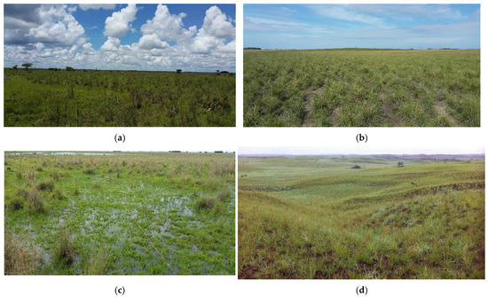
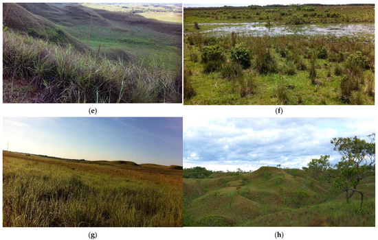
Figure 1.
Physiography in grasslands and meadows of the alliances: (a) Paspalion carinato—pectinati in High plain; (b) Steinchismo laxae—Andropogonion bicornis in Alluvial plain; (c) Rhynchosporo barbatae—Andropogonion virgarti in Alluvial plain; (d) Axonopodo aurei-Trachypogonion spicati in High plain; (e) Paspalo pectinati—Axonopodion aurei in High plain; (f) Andropogono virgati—Axonopodion ancepitis in Alluvial plain; (g) Hyptio brachiatae—Trachypogonion spicati in High plain; (h) Bowdichio virgilioidis—Curatellion americanae in High plain.
4.2. Dataset
For the construction of the model, 292 georeferenced grassland surveys were considered ([32,96]; Table A1). The categories of weighted richness were established according to [97] and based on the natural break classification of the number of species recorded in each survey, where the data were grouped according to their inherent characteristics to define intervals of similar values and maximize the differences between classes [98]. This approach, in addition to providing a more uniform structure to a set of surveys derived from various studies (floristic, geobotanical, phytosociological, ecological, etc.), allows for a preliminary understanding of how richness values vary and segregate hierarchically within syntaxonomic arrangements, without the variability in the number of surveys per physiographic unit significantly interfering with their interpretation at the regional scale.
Reclassifying numerical species richness into ordinal categories such as paucispecific, oligospecific, mesospecific, and polyspecific offers several advantages, particularly when working with small datasets and exploring ecological hypotheses. It simplifies the analysis by reducing noise and making models statistically more robust, especially for ordinal regression methods that are better suited for limited samples. Additionally, it enhances ecological interpretation by capturing qualitative shifts in biodiversity and linking them to specific climatic and edaphic thresholds. This approach also mitigates issues related to sparse data in certain richness ranges, enabling the detection of broader patterns. Finally, it facilitates communication of results, as the ordinal categories are more intuitive and actionable for conservation and management purposes.
Species richness was reclassified into ordinal categories using geometric intervals. It is justified from both statistical and ecological perspectives, especially when working with small datasets. Geometric intervals divide data proportionally on a scale that reflects the nonlinear patterns typical of ecological variables. This approach emphasizes relative differences at lower richness levels, where biodiversity changes have greater ecological significance, while smoothing variability at higher levels. It ensures a balanced distribution of categories, preventing overrepresentation of certain ranges, which is particularly important for small datasets. Additionally, geometric intervals provide a consistent and transparent method for classification, enhancing the interpretability and comparability of results.
The percentage of bare soil data was collected directly in the field, slope data were extracted from the processing of the Shuttle Radar Topography Mission (SRTM v.3) 30 m digital elevation model, climate data for temperature and precipitation were extracted from WorldClim bioclimatic models [99], and other data related to physiography, relief, and edaphic characteristics were obtained from Colombia’s geopedology map at a 1:100,000 scale [100].
4.3. Statistical Framework
As the response variable, plant species richness in the Orinoquia grasslands was used, classified into four alpha diversity categories: paucispecific, oligospecific, mesospecific, and polyspecific. Based on the structure of the ordinal dependent variable, the negative log−log (−log(−log(x))) link function was established, as it is typically applied when lower categories are more likely in the variable’s distribution [101]. The analysis included both ordinal and scale covariates. The ordinal covariates considered were soil depth, with categories ranging from shallow to deep; soil texture, from fine to coarse; soil moisture regime, from ustic to aquic; and three levels of aluminum content. The scale covariates included the percentage of bare soil, annual mean temperature, monthly maximum temperature, monthly minimum temperature, annual mean precipitation, monthly maximum precipitation, monthly minimum precipitation, and slope percentage [32].
A multivariate approach was employed for data analysis. Initially, a bivariate exploratory analysis was conducted using Spearman’s Rho to assess the correlation between scale covariates and weighted richness. For ordinal covariates, Kendall’s Tau-b was applied. Only those covariates with a two-tailed bivariate significance level of less than 0.05 were selected for multivariate analysis. Additional exploratory analyses were then performed through bivariate and multivariate ordinal logistic regressions. Before conducting the exploratory ordinal regressions, a Variance Inflation Factor (VIF) test was performed to evaluate multicollinearity among the predictor variables. High multicollinearity can inflate standard errors, reduce the statistical significance of predictors, and complicate the interpretation of regression coefficients, potentially leading to unreliable models. Variables with VIF values exceeding 10, a commonly used threshold indicating severe multicollinearity, were excluded to improve model stability and robustness.
In the multivariate regressions, variables showing statistical significance in the bivariate regressions were included. The final variable selection was based on Wald statistics. Covariates that did not contribute significantly to the regression were excluded from the final model. The final ordinal regression model included the selected covariates and was evaluated using −2 log likelihood (−2LL) and the Chi-square test, comparing the initial and final model fits. Cox and Snell’s R2 and Nagelkerke’s R2 values indicated the model’s validity in predicting variation in weighted richness. A two-tailed bivariate significance of <0.05 with weighted richness was used as the inclusion criterion for an independent variable in the multivariate analysis. The correlation of scale covariates was estimated with Spearman’s rho, while the correlation of ordinal covariates was assessed using Kendall’s Tau-b. Factors, as nominal variables, were not considered in the bivariate exploratory analysis. To compare the behavior of regression coefficients, complementary exploratory analyses were conducted with bivariate and multivariate ordinal logistic regressions, where variables meeting the established statistical significance during the bivariate analysis were included. Once the variables to be included in the final model were determined based on the statistical significance estimated during the bivariate and multivariate exploratory analyses, an ordinal regression was conducted [32,102].
5. Conclusions
Only through a comprehensive and multidimensional perspective of biodiversity it is possible to design and implement effective conservation actions that are appropriate to the sociocultural context of the territories. Over the past decade, there has been a notable global interest in deepening the understanding of grassland richness, highlighting the ecological and sociocultural implications that must be considered for its conservation [103,104,105,106]; consequently, accurate characterization (both biophysical and cultural) serves as the primary starting point for the development of plans and actions aimed at these purposes.
Multiple physical processes operate at different scales in nature, creating gradients that limit the extent and meanings of the ecological expression of species and, subsequently, of plant communities. It is possible that these gradients largely exceed the statistical models that aim to explain the vegetation–environment relationships [107]. While phytocenoses are a direct response to the characteristics defining the habitat assemblages present in the Colombian Llanos, their ecogeographical reach and biotic uniqueness cannot be inferred under the premise of regional homogeneity.
Our findings support the hypothesis that environmental factors and soil physical properties play a significant role in the patterns of plant species richness in grasslands. In this regard, similar relationships have been described in various regions of Africa, with particular emphasis on how nitrogen levels, along with soil texture and, subsequently, moisture, influence species diversity [108]. In our study area, soil depth, soil moisture as a result of its structural attributes (texture), and the percentage of bare soil are the key factors that help outline and explain a regional pattern regarding the prevalence of grasslands tending toward oligospecific to mesospecific conditions. This pattern is comparable to other grassland-dominated areas, such as the páramos, and to a lesser extent, the casmophytic savannas of the Guayana region.
This contribution underscores the relevance of articulating and combining the floristic and phytosociological characterization of grassland vegetation with the fundamental attributes of the natural environment for constructing predictive models of species richness. Additionally, it emphasizes the importance of conducting regional and local studies on the flora, vegetation, and ecology of the Colombian eastern extrandine grasslands, which possess a biogeographical and paleoecological significance that remains unresolved. Although the use of such models is primarily associated with specific studies aimed at addressing issues related to Alpha diversity and, to a lesser extent, Beta diversity, they can also be extended to strengthen ecological niche models, accurately assess the biotic significance of territories, analyze the spatial and temporal dynamics of plant communities, and, of course, identify new areas designated for conservation. In this regard, the data and information used in this contribution were pivotal in supporting the process of declaring a new national natural park, the Serranía de Manacacías National Natural Park (Meta department), and are currently being used in the process of establishing new conservation areas such as the Arauca Wetlands (Arauca department) and the Transitional Forests of Cumaribo (Vichada department).
Author Contributions
Conceptualization, methodology and formal analysis V.M.-C. and L.N.; investigation V.M.-C., L.N. and O.R. data curation V.M.-C., L.N. and O.R.; writing—original draft preparation V.M.-C. and L.N.; writing—review and editing V.M.-C., L.N., O.R. and D.S.-M.; visualization V.M.-C., L.N., O.R. and D.S.-M. All authors have read and agreed to the published version of the manuscript.
Funding
This research received no external funding, and the APC was founded by Institutional Open Access Program (IOAP): Complutense University of Madrid. Author Voucher discount code (02797156366c631a).
Data Availability Statement
All data supporting the reported results are included in the paper.
Acknowledgments
We would like to thank Gerardo Aymard, Francisco Castro-Lima, and Francisco Mijares for their vegetation plots, as well as their support during fieldwork and the taxonomic identification of species. Special thanks to Diego Giraldo-Cañas (COL) for his valuable, timely, and insightful comments on the preliminary version of this manuscript and to Igal Berenstein for the proofreading.
Conflicts of Interest
The authors declare no conflicts of interest.
Appendix A
Table A1.
Geographic location of the Colombian Orinoquian grassland plots. Area 10 × 10 m.
Table A1.
Geographic location of the Colombian Orinoquian grassland plots. Area 10 × 10 m.
| Id_Plot | Plot | Physiography | Location | Spp. No. | pH | Parent Material | Precipitation mm | Slope | Vegetation Cover (%) | Bare Soil (%) | Longitude | Latitude | Altitude |
|---|---|---|---|---|---|---|---|---|---|---|---|---|---|
| 1 | S.11 | High plain | Manacacías | 9 | 4.0–5.5 | Clay alluvium | >2300 | >2 | 98 | 2 | 72°27′16.95″ | 3°29′52.3″ | 172 |
| 2 | S.13 | High plain | Manacacías | 10 | 4.0–5.5 | Clay alluvium | >2300 | >2 | 99 | 1 | 72°27′16.97″ | 3°29′52.3″ | 172 |
| 3 | S.15 | High plain | Manacacías | 14 | 4.0–5.5 | Clay alluvium | >2300 | >2 | 99 | 1 | 72°27′16.99″ | 3°29′52.3″ | 172 |
| 4 | S.17 | High plain | Manacacías | 10 | 4.0–5.5 | Clay alluvium | >2300 | >2 | 94 | 6 | 72°27′16.1″ | 3°29′52.3″ | 172 |
| 5 | S.18 | High plain | Manacacías | 15 | 4.0–5.5 | Clay alluvium | >2300 | >2 | 98 | 2 | 72°27′16.1″ | 3°29′52.3″ | 172 |
| 6 | S.14 | High plain | Manacacías | 11 | 4.0–5.5 | Clay alluvium | >2300 | >2 | 100 | 0 | 72°27′16.98″ | 3°29′52.3″ | 172 |
| 7 | S.12 | High plain | Manacacías | 17 | 4.0–5.5 | Clay alluvium | >2300 | >2 | 99 | 1 | 72°27′16.96″ | 3°29′52.3″ | 172 |
| 8 | S.39 | High plain | Manacacías | 5 | 4.0–5.5 | Clay alluvium | >2300 | >2 | 96 | 4 | 72°24′16.12″ | 3°26′45.02″ | 169 |
| 9 | S.21 | High plain | Manacacías | 11 | 4.0–5.5 | Clay alluvium | >2300 | >2 | 96 | 4 | 72°24′16.11″ | 3°26′46.32″ | 166 |
| 10 | S.22 | High plain | Manacacías | 8 | 4.0–5.5 | Clay alluvium | >2300 | >2 | 100 | 0 | 72°24′16.11″ | 3°26′46.32″ | 166 |
| 11 | S.23 | High plain | Manacacías | 10 | 4.0–5.5 | Clay alluvium | >2300 | >2 | 99 | 1 | 72°24′16.11″ | 3°26′46.32″ | 166 |
| 12 | S.24 | High plain | Manacacías | 7 | 4.0–5.5 | Clay alluvium | >2300 | >2 | 100 | 0 | 72°24′16.11″ | 3°26′46.32″ | 166 |
| 13 | S.25 | High plain | Manacacías | 7 | 4.0–5.5 | Clay alluvium | >2300 | >2 | 100 | 0 | 72°24′16.11″ | 3°26′46.32″ | 166 |
| 14 | S.26 | High plain | Manacacías | 7 | 4.0–5.5 | Clay alluvium | >2300 | >2 | 96 | 4 | 72°24′16.11″ | 3°26′46.32″ | 162 |
| 15 | S.1 | High plain | Manacacías | 8 | 4.0–5.5 | Clay alluvium | >2300 | >2 | 95 | 5 | 72°27′16.85″ | 3°29′50.53″ | 169 |
| 16 | S.2 | High plain | Manacacías | 7 | 4.0–5.5 | Clay alluvium | >2300 | >2 | 92 | 8 | 72°27′16.86″ | 3°29′50.53″ | 169 |
| 17 | S.10 | High plain | Manacacías | 7 | 4.0–5.5 | Clay alluvium | >2300 | >2 | 96 | 4 | 72°27′16.94″ | 3°29′50.53″ | 170 |
| 18 | S.5 | High plain | Manacacías | 7 | 4.0–5.5 | Clay alluvium | >2300 | >2 | 99 | 1 | 72°27′16.89″ | 3°29′50.53″ | 169 |
| 19 | S.6 | High plain | Manacacías | 4 | 4.0–5.5 | Clay alluvium | >2300 | >2 | 92 | 8 | 72°27′16.9″ | 3°29′50.53″ | 170 |
| 20 | S.7 | High plain | Manacacías | 5 | 4.0–5.5 | Clay alluvium | >2300 | >2 | 100 | 0 | 72°27′16.91″ | 3°29′50.53″ | 170 |
| 21 | S.9 | High plain | Manacacías | 5 | 4.0–5.5 | Clay alluvium | >2300 | >2 | 99 | 1 | 72°27′16.93″ | 3°29′50.53″ | 170 |
| 22 | S.19 | High plain | Manacacías | 4 | 4.0–5.5 | Clay alluvium | >2300 | >2 | 28 | 72 | 72°27′16.1″ | 3°29′52.3″ | 172 |
| 23 | S.27 | High plain | Manacacías | 8 | 4.0–5.5 | Clay alluvium | >2300 | >2 | 100 | 0 | 72°24′16.11″ | 3°26′46.32″ | 162 |
| 24 | S.30 | High plain | Manacacías | 7 | 4.0–5.5 | Clay alluvium | >2300 | >2 | 95 | 5 | 72°24′16.11″ | 3°26′46.32″ | 162 |
| 25 | S.3 | High plain | Manacacías | 6 | 4.0–5.5 | Clay alluvium | >2300 | >2 | 95 | 5 | 72°27′16.87″ | 3°29′50.53″ | 169 |
| 26 | S.8 | High plain | Manacacías | 4 | 4.0–5.5 | Clay alluvium | >2300 | >2 | 100 | 0 | 72°27′16.92″ | 3°29′50.53″ | 170 |
| 27 | S.61 | High plain | Manacacías | 8 | 4.0–5.5 | Clay alluvium | >2300 | >2 | 99 | 1 | 72°26′16.15″ | 3°30′35.75″ | 183 |
| 28 | S.64 | High plain | Manacacías | 8 | 4.0–5.5 | Clay alluvium | >2300 | >2 | 99 | 1 | 72°26′16.15″ | 3°30′35.75″ | 183 |
| 29 | S.65 | High plain | Manacacías | 7 | 4.0–5.5 | Clay alluvium | >2300 | >2 | 100 | 0 | 72°26′16.15″ | 3°30′35.75″ | 183 |
| 30 | S.66 | High plain | Manacacías | 7 | 4.0–5.5 | Clay alluvium | >2300 | >2 | 99 | 1 | 72°26′16.15″ | 3°30′35.75″ | 180 |
| 31 | S.67 | High plain | Manacacías | 9 | 4.0–5.5 | Clay alluvium | >2300 | >2 | 88 | 12 | 72°26′16.15″ | 3°30′35.75″ | 180 |
| 32 | S.71 | High plain | Manacacías | 16 | 4.0–5.5 | Clay alluvium | >2300 | >2 | 100 | 0 | 72°26′16.16″ | 3°30′29.27″ | 200 |
| 33 | S.73 | High plain | Manacacías | 19 | 4.0–5.5 | Clay alluvium | >2300 | >2 | 100 | 0 | 72°26′16.16″ | 3°30′29.27″ | 200 |
| 34 | S.75 | High plain | Manacacías | 12 | 4.0–5.5 | Clay alluvium | >2300 | >2 | 100 | 0 | 72°26′16.16″ | 3°30′29.27″ | 200 |
| 35 | S.101 | High plain | Manacacías | 16 | 4.0–5.5 | Clay alluvium | >2300 | >2 | 99 | 1 | 72°26′16.19″ | 3°30′29.27″ | 186 |
| 36 | S.102 | High plain | Manacacías | 21 | 4.0–5.5 | Clay alluvium | >2300 | >2 | 98 | 2 | 72°26′16.19″ | 3°30′29.27″ | 186 |
| 37 | S.103 | High plain | Manacacías | 13 | 4.0–5.5 | Clay alluvium | >2300 | >2 | 99 | 1 | 72°26′16.19″ | 3°30′29.27″ | 186 |
| 38 | S.104 | High plain | Manacacías | 20 | 4.0–5.5 | Clay alluvium | >2300 | >2 | 99 | 1 | 72°26′16.19″ | 3°30′29.27″ | 186 |
| 39 | S.105 | High plain | Manacacías | 21 | 4.0–5.5 | Clay alluvium | >2300 | >2 | 96 | 4 | 72°26′16.19″ | 3°30′29.27″ | 186 |
| 40 | S.107 | High plain | Manacacías | 17 | 4.0–5.5 | Clay alluvium | >2300 | >2 | 99 | 1 | 72°26′16.19″ | 3°30′29.27″ | 186 |
| 41 | S.161 | High plain | Manacacías | 15 | 4.0–5.5 | Clay alluvium | >2300 | >2 | 98 | 2 | 73°2′16.25″ | 3°52′50.1″ | 180 |
| 42 | S.162 | High plain | Manacacías | 21 | 4.0–5.5 | Clay alluvium | >2300 | >2 | 100 | 0 | 73°3′16.25″ | 2°27′10.54″ | 180 |
| 43 | S.163 | High plain | Manacacías | 13 | 4.0–5.5 | Clay alluvium | >2300 | >2 | 53 | 47 | 73°3′16.25″ | 2°27′10.54″ | 180 |
| 44 | S.164 | High plain | Manacacías | 20 | 4.0–5.5 | Clay alluvium | >2300 | >2 | 98 | 2 | 73°2′16.25″ | 3°52′50.1″ | 180 |
| 45 | S.165 | High plain | Manacacías | 21 | 4.0–5.5 | Clay alluvium | >2300 | >2 | 96 | 4 | 73°46′16.25″ | 2°4′9.7″ | 180 |
| 46 | S.167 | High plain | Manacacías | 17 | 4.0–5.5 | Clay alluvium | >2300 | >2 | 99 | 1 | 73°46′16.25″ | 2°4′9.7″ | 180 |
| 47 | S.108 | High plain | Manacacías | 15 | 4.0–5.5 | Clay alluvium | >2300 | >2 | 100 | 0 | 72°26′16.19″ | 3°30′29.27″ | 186 |
| 48 | S.109 | High plain | Manacacías | 23 | 4.0–5.5 | Clay alluvium | >2300 | >2 | 98 | 2 | 72°26′16.19″ | 3°30′29.27″ | 186 |
| 49 | S.110 | High plain | Manacacías | 16 | 4.0–5.5 | Clay alluvium | >2300 | >2 | 100 | 0 | 72°33′16.19″ | 3°32′19.4″ | 186 |
| 50 | S.168 | High plain | Manacacías | 15 | 4.0–5.5 | Clay alluvium | >2300 | >2 | 100 | 0 | 73°46′16.25″ | 2°4′9.7″ | 180 |
| 51 | S.169 | High plain | Manacacías | 23 | 4.0–5.5 | Clay alluvium | >2300 | >2 | 98 | 2 | 73°46′16.25″ | 2°4′9.7″ | 180 |
| 52 | S.170 | High plain | Manacacías | 16 | 4.0–5.5 | Clay alluvium | >2300 | >2 | 100 | 0 | 73°12′16.25″ | 2°28′6.28″ | 180 |
| 53 | S.160 | High plain | Manacacías | 7 | 4.0–5.5 | Clay alluvium | >2300 | >2 | 99 | 1 | 73°2′16.24″ | 3°52′50.1″ | 216 |
| 54 | S.122 | High plain | Manacacías | 20 | 4.0–5.5 | Clay alluvium | >2300 | >2 | 98 | 2 | 72°23′16.21″ | 3°29′20.47″ | 169 |
| 55 | S.124 | High plain | Manacacías | 15 | 4.0–5.5 | Clay alluvium | >2300 | >2 | 100 | 0 | 72°23′16.21″ | 3°29′20.47″ | 169 |
| 56 | S.121 | High plain | Manacacías | 17 | 4.0–5.5 | Clay alluvium | >2300 | >2 | 100 | 0 | 72°23′16.21″ | 3°29′20.47″ | 169 |
| 57 | S.126 | High plain | Manacacías | 16 | 4.0–5.5 | Clay alluvium | >2300 | >2 | 100 | 0 | 72°23′16.21″ | 3°29′20.47″ | 169 |
| 58 | S.128 | High plain | Manacacías | 16 | 4.0–5.5 | Clay alluvium | >2300 | >2 | 100 | 0 | 72°23′16.21″ | 3°29′20.47″ | 169 |
| 59 | S.129 | High plain | Manacacías | 16 | 4.0–5.5 | Clay alluvium | >2300 | >2 | 98 | 2 | 72°23′16.21″ | 3°29′17.2″ | 169 |
| 60 | S.123 | High plain | Manacacías | 15 | 4.0–5.5 | Clay alluvium | >2300 | >2 | 100 | 0 | 72°23′16.21″ | 3°29′20.47″ | 169 |
| 61 | S.152 | High plain | Manacacías | 14 | 4.0–5.5 | Clay alluvium | >2300 | >2 | 100 | 0 | 72°28′16.24″ | 3°35′24.4″ | 216 |
| 62 | S.154 | High plain | Manacacías | 10 | 4.0–5.5 | Clay alluvium | >2300 | >2 | 99 | 1 | 72°21′16.24″ | 2°38′31.37″ | 216 |
| 63 | S.157 | High plain | Manacacías | 6 | 4.0–5.5 | Clay alluvium | >2300 | >2 | 100 | 0 | 72°21′16.24″ | 2°38′31.37″ | 216 |
| 64 | S.158 | High plain | Manacacías | 8 | 4.0–5.5 | Clay alluvium | >2300 | >2 | 100 | 0 | 72°25′16.24″ | 2°30′55.39″ | 216 |
| 65 | S.153 | High plain | Manacacías | 13 | 4.0–5.5 | Clay alluvium | >2300 | >2 | 100 | 0 | 72°21′16.24″ | 2°38′31.37″ | 216 |
| 66 | S.151 | High plain | Manacacías | 11 | 4.0–5.5 | Clay alluvium | >2300 | >2 | 99 | 1 | 72°28′16.24″ | 3°35′23.7″ | 216 |
| 67 | S.155 | High plain | Manacacías | 12 | 4.0–5.5 | Clay alluvium | >2300 | >2 | 99 | 1 | 72°21′16.24″ | 2°38′31.37″ | 216 |
| 68 | S.156 | High plain | Manacacías | 14 | 4.0–5.5 | Clay alluvium | >2300 | >2 | 100 | 0 | 72°21′16.24″ | 2°38′31.37″ | 216 |
| 69 | S.125 | High plain | Manacacías | 21 | 4.0–5.5 | Clay alluvium | >2300 | >2 | 100 | 0 | 72°23′16.21″ | 3°29′20.47″ | 169 |
| 70 | S.127 | High plain | Manacacías | 19 | 4.0–5.5 | Clay alluvium | >2300 | >2 | 98 | 2 | 72°23′16.21″ | 3°29′20.47″ | 169 |
| 71 | S.159 | High plain | Manacacías | 10 | 4.0–5.5 | Clay alluvium | >2300 | >2 | 100 | 0 | 72°25′16.24″ | 2°30′55.39″ | 216 |
| 72 | S.41 | High plain | Manacacías | 14 | 4.0–5.5 | Clay alluvium | >2300 | >2 | 90 | 10 | 72°23′16.13″ | 3°27′19.08″ | 164 |
| 73 | S.42 | High plain | Manacacías | 11 | 4.0–5.5 | Clay alluvium | >2300 | >2 | 94 | 6 | 72°23′16.13″ | 3°27′19.08″ | 164 |
| 74 | S.43 | High plain | Manacacías | 18 | 4.0–5.5 | Clay alluvium | >2300 | >2 | 91 | 9 | 72°23′16.13″ | 3°27′19.08″ | 164 |
| 75 | S.44 | High plain | Manacacías | 16 | 4.0–5.5 | Clay alluvium | >2300 | >2 | 96 | 4 | 72°23′16.13″ | 3°27′19.08″ | 164 |
| 76 | S.45 | High plain | Manacacías | 12 | 4.0–5.5 | Clay alluvium | >2300 | >2 | 98 | 2 | 72°23′16.13″ | 3°27′19.08″ | 164 |
| 77 | S.46 | High plain | Manacacías | 10 | 4.0–5.5 | Clay alluvium | >2300 | >2 | 86 | 14 | 72°23′16.13″ | 3°27′19.08″ | 169 |
| 78 | S.49 | High plain | Manacacías | 12 | 4.0–5.5 | Clay alluvium | >2300 | >2 | 89 | 11 | 72°23′16.13″ | 3°27′19.08″ | 169 |
| 79 | S.51 | High plain | Manacacías | 7 | 4.0–5.5 | Clay alluvium | >2300 | >2 | 67 | 33 | 72°23′16.14″ | 3°27′18.14″ | 180 |
| 80 | S.52 | High plain | Manacacías | 11 | 4.0–5.5 | Clay alluvium | >2300 | >2 | 72 | 28 | 72°23′16.14″ | 3°27′18.14″ | 180 |
| 81 | S.54 | High plain | Manacacías | 7 | 4.0–5.5 | Clay alluvium | >2300 | >2 | 87 | 13 | 72°23′16.14″ | 3°27′18.14″ | 180 |
| 82 | S.55 | High plain | Manacacías | 9 | 4.0–5.5 | Clay alluvium | >2300 | >2 | 85 | 15 | 72°23′16.14″ | 3°27′18.14″ | 180 |
| 83 | S.58 | High plain | Manacacías | 10 | 4.0–5.5 | Clay alluvium | >2300 | >2 | 90 | 10 | 72°23′16.14″ | 3°27′18.14″ | 183 |
| 84 | S.59 | High plain | Manacacías | 7 | 4.0–5.5 | Clay alluvium | >2300 | >2 | 91 | 9 | 72°23′16.14″ | 3°27′18.14″ | 183 |
| 85 | S.31 | High plain | Manacacías | 11 | 4.0–5.5 | Clay alluvium | >2300 | >2 | 62 | 38 | 72°24′16.12″ | 3°26′45.02″ | 164 |
| 86 | S.36 | High plain | Manacacías | 8 | 4.0–5.5 | Clay alluvium | >2300 | >2 | 81 | 19 | 72°24′16.12″ | 3°26′45.02″ | 169 |
| 87 | S.38 | High plain | Manacacías | 7 | 4.0–5.5 | Clay alluvium | >2300 | >2 | 95 | 5 | 72°24′16.12″ | 3°26′45.02″ | 169 |
| 88 | S.40 | High plain | Manacacías | 7 | 4.0–5.5 | Clay alluvium | >2300 | >2 | 91 | 9 | 72°24′16.12″ | 3°26′45.02″ | 169 |
| 89 | S.86 | High plain | Manacacías | 15 | 4.0–5.5 | Clay alluvium | >2300 | >2 | 97 | 3 | 72°23′16.17″ | 3°29′20.47″ | 173 |
| 90 | S.111 | High plain | Manacacías | 17 | 4.0–5.5 | Clay alluvium | >2300 | >2 | 92 | 8 | 72°36′16.2″ | 3°32′18.7″ | 186 |
| 91 | S.113 | High plain | Manacacías | 17 | 4.0–5.5 | Clay alluvium | >2300 | >2 | 97 | 3 | 72°36′16.2″ | 3°34′28.93″ | 186 |
| 92 | S.116 | High plain | Manacacías | 9 | 4.0–5.5 | Clay alluvium | >2300 | >2 | 95 | 5 | 72°28′16.2″ | 3°37′34.8″ | 186 |
| 93 | S.117 | High plain | Manacacías | 8 | 4.0–5.5 | Clay alluvium | >2300 | >2 | 85 | 15 | 72°28′16.2″ | 3°38′13.3″ | 186 |
| 94 | S.143 | High plain | Manacacías | 14 | 4.0–5.5 | Clay alluvium | >2300 | >2 | 92 | 8 | 72°28′16.23″ | 3°35′40.6″ | 197 |
| 95 | S.118 | High plain | Manacacías | 13 | 4.0–5.5 | Clay alluvium | >2300 | >2 | 94 | 6 | 72°29′16.2″ | 3°38′24.5″ | 186 |
| 96 | S.119 | High plain | Manacacías | 14 | 4.0–5.5 | Clay alluvium | >2300 | >2 | 96 | 4 | 72°23′16.2″ | 3°29′20.47″ | 186 |
| 97 | S.120 | High plain | Manacacías | 25 | 4.0–5.5 | Clay alluvium | >2300 | >2 | 81 | 19 | 72°23′16.2″ | 3°29′20.47″ | 186 |
| 98 | S.149 | High plain | Manacacías | 12 | 4.0–5.5 | Clay alluvium | >2300 | >2 | 88 | 12 | 72°35′16.23″ | 3°35′45.6″ | 197 |
| 99 | S.130 | High plain | Manacacías | 14 | 4.0–5.5 | Clay alluvium | >2300 | >2 | 98 | 2 | 72°23′16.21″ | 3°29′17.2″ | 169 |
| 100 | S.50 | High plain | Manacacías | 12 | 4.0–5.5 | Clay alluvium | >2300 | >2 | 92 | 8 | 72°23′16.13″ | 3°27′19.08″ | 169 |
| 101 | S.57 | High plain | Manacacías | 9 | 4.0–5.5 | Clay alluvium | >2300 | >2 | 95 | 5 | 72°23′16.14″ | 3°27′18.14″ | 183 |
| 102 | S.79 | High plain | Manacacías | 10 | 4.0–5.5 | Clay alluvium | >2300 | >2 | 84 | 16 | 72°26′16.16″ | 3°30′29.27″ | 199 |
| 103 | S.70 | High plain | Manacacías | 8 | 4.0–5.5 | Clay alluvium | >2300 | >2 | 88 | 12 | 72°26′16.15″ | 3°30′35.75″ | 200 |
| 104 | S.72 | High plain | Manacacías | 12 | 4.0–5.5 | Clay alluvium | >2300 | >2 | 95 | 5 | 72°26′16.16″ | 3°30′29.27″ | 200 |
| 105 | S.74 | High plain | Manacacías | 11 | 4.0–5.5 | Clay alluvium | >2300 | >2 | 94 | 6 | 72°26′16.16″ | 3°30′29.27″ | 200 |
| 106 | S.76 | High plain | Manacacías | 14 | 4.0–5.5 | Clay alluvium | >2300 | >2 | 95 | 5 | 72°26′16.16″ | 3°30′29.27″ | 199 |
| 107 | S.80 | High plain | Manacacías | 8 | 4.0–5.5 | Clay alluvium | >2300 | >2 | 90 | 10 | 72°26′16.16″ | 3°30′29.27″ | 167 |
| 108 | S.138 | High plain | Manacacías | 12 | 4.0–5.5 | Clay alluvium | >2300 | >2 | 97 | 3 | 72°23′16.22″ | 3°29′17.2″ | 177 |
| 109 | S.139 | High plain | Manacacías | 11 | 4.0–5.5 | Clay alluvium | >2300 | >2 | 80 | 20 | 72°36′16.22″ | 3°34′18.4″ | 177 |
| 110 | S.136 | High plain | Manacacías | 16 | 4.0–5.5 | Clay alluvium | >2300 | >2 | 96 | 4 | 72°23′16.22″ | 3°29′17.2″ | 177 |
| 111 | S.132 | High plain | Manacacías | 17 | 4.0–5.5 | Clay alluvium | >2300 | >2 | 93 | 7 | 72°23′16.22″ | 3°29′17.2″ | 177 |
| 112 | S.133 | High plain | Manacacías | 13 | 4.0–5.5 | Clay alluvium | >2300 | >2 | 99 | 1 | 72°23′16.22″ | 3°29′17.2″ | 177 |
| 113 | S.134 | High plain | Manacacías | 14 | 4.0–5.5 | Clay alluvium | >2300 | >2 | 80 | 20 | 72°23′16.22″ | 3°29′17.2″ | 177 |
| 114 | S.135 | High plain | Manacacías | 17 | 4.0–5.5 | Clay alluvium | >2300 | >2 | 97 | 3 | 72°23′16.22″ | 3°29′17.2″ | 177 |
| 115 | S.137 | High plain | Manacacías | 17 | 4.0–5.5 | Clay alluvium | >2300 | >2 | 94 | 6 | 72°23′16.22″ | 3°29′17.2″ | 177 |
| 116 | S.77 | High plain | Manacacías | 12 | 4.0–5.5 | Clay alluvium | >2300 | >2 | 97 | 3 | 72°26′16.16″ | 3°30′29.27″ | 199 |
| 117 | S.141 | High plain | Manacacías | 15 | 4.0–5.5 | Clay alluvium | >2300 | >2 | 97 | 3 | 72°36′16.23″ | 3°34′20.7″ | 197 |
| 118 | S.142 | High plain | Manacacías | 11 | 4.0–5.5 | Clay alluvium | >2300 | >2 | 92 | 8 | 72°28′16.23″ | 3°33′42.5″ | 197 |
| 119 | S.144 | High plain | Manacacías | 13 | 4.0–5.5 | Clay alluvium | >2300 | >2 | 92 | 8 | 72°28′16.23″ | 3°35′38.9″ | 197 |
| 120 | S.20 | High plain | Manacacías | 8 | 4.0–5.5 | Clay alluvium | >2300 | >2 | 96 | 4 | 72°27′16.1″ | 3°29′52.3″ | 172 |
| 121 | S.85 | High plain | Manacacías | 9 | 4.0–5.5 | Clay alluvium | >2300 | >2 | 90 | 10 | 72°23′16.17″ | 3°29′20.47″ | 173 |
| 122 | S.82 | High plain | Manacacías | 13 | 4.0–5.5 | Clay alluvium | >2300 | >2 | 94 | 6 | 72°23′16.17″ | 3°29′20.47″ | 167 |
| 123 | S.87 | High plain | Manacacías | 13 | 4.0–5.5 | Clay alluvium | >2300 | >2 | 97 | 3 | 72°23′16.17″ | 3°29′20.47″ | 173 |
| 124 | S.89 | High plain | Manacacías | 11 | 4.0–5.5 | Clay alluvium | >2300 | >2 | 91 | 9 | 72°23′16.17″ | 3°29′20.47″ | 173 |
| 125 | S.98 | High plain | Manacacías | 6 | 4.0–5.5 | Clay alluvium | >2300 | >2 | 87 | 13 | 72°23′16.18″ | 3°29′17.2″ | 170 |
| 126 | S.16 | High plain | Manacacías | 6 | 4.0–5.5 | Clay alluvium | >2300 | >2 | 80 | 20 | 72°27′16.1″ | 3°29′52.3″ | 172 |
| 127 | S.32 | High plain | Manacacías | 9 | 4.0–5.5 | Clay alluvium | >2300 | >2 | 96 | 4 | 72°24′16.12″ | 3°26′45.02″ | 164 |
| 128 | S.35 | High plain | Manacacías | 5 | 4.0–5.5 | Clay alluvium | >2300 | >2 | 92 | 8 | 72°24′16.12″ | 3°26′45.02″ | 164 |
| 129 | S.37 | High plain | Manacacías | 5 | 4.0–5.5 | Clay alluvium | >2300 | >2 | 96 | 4 | 72°24′16.12″ | 3°26′45.02″ | 169 |
| 130 | S.81 | High plain | Manacacías | 10 | 4.0–5.5 | Clay alluvium | >2300 | >2 | 87 | 13 | 72°23′16.17″ | 3°29′20.47″ | 167 |
| 131 | S.90 | High plain | Manacacías | 8 | 4.0–5.5 | Clay alluvium | >2300 | >2 | 95 | 5 | 72°23′16.17″ | 3°29′20.47″ | 174 |
| 132 | S.145 | High plain | Manacacías | 14 | 4.0–5.5 | Clay alluvium | >2300 | >2 | 93 | 7 | 72°28′16.23″ | 3°35′34.6″ | 197 |
| 133 | S.146 | High plain | Manacacías | 13 | 4.0–5.5 | Clay alluvium | >2300 | >2 | 97 | 3 | 72°28′16.23″ | 3°35′37″ | 197 |
| 134 | S.147 | High plain | Manacacías | 14 | 4.0–5.5 | Clay alluvium | >2300 | >2 | 99 | 1 | 72°33′16.23″ | 3°31′44″ | 197 |
| 135 | S.148 | High plain | Manacacías | 15 | 4.0–5.5 | Clay alluvium | >2300 | >2 | 96 | 4 | 72°35′16.23″ | 3°35′46.3″ | 197 |
| 136 | S.150 | High plain | Manacacías | 10 | 4.0–5.5 | Clay alluvium | >2300 | >2 | 85 | 15 | 72°35′16.23″ | 3°35′46.3″ | 197 |
| 137 | S.178 | High plain | Manacacías | 5 | 4.0–5.5 | Clay alluvium | >2300 | >2 | 96 | 4 | 72°33′16.26″ | 3°32′19.4″ | 234 |
| 138 | S.183 | High plain | Manacacías | 10 | 4.0–5.5 | Clay alluvium | >2300 | >2 | 82 | 18 | 72°36′16.27″ | 3°32′18.7″ | 230 |
| 139 | S.184 | High plain | Manacacías | 10 | 4.0–5.5 | Clay alluvium | >2300 | >2 | 92 | 8 | 72°28′16.27″ | 3°37′34.8″ | 201 |
| 140 | S.185 | High plain | Manacacías | 10 | 4.0–5.5 | Clay alluvium | >2300 | >2 | 88 | 12 | 72°28′16.27″ | 3°38′13.3″ | 208 |
| 141 | S.188 | High plain | Manacacías | 11 | 4.0–5.5 | Clay alluvium | >2300 | >2 | 85 | 15 | 72°36′16.27″ | 3°32′18.6″ | 222 |
| 142 | S.33 | High plain | Manacacías | 8 | 4.0–5.5 | Clay alluvium | >2300 | >2 | 96 | 4 | 72°24′16.12″ | 3°26′45.02″ | 164 |
| 143 | S.93 | High plain | Manacacías | 7 | 4.0–5.5 | Clay alluvium | >2300 | >2 | 85 | 15 | 72°23′16.18″ | 3°29′17.2″ | 174 |
| 144 | S.114 | High plain | Manacacías | 11 | 4.0–5.5 | Clay alluvium | >2300 | >2 | 91 | 9 | 72°36′16.2″ | 3°34′30.47″ | 186 |
| 145 | S.63 | High plain | Manacacías | 8 | 4.0–5.5 | Clay alluvium | >2300 | >2 | 97 | 3 | 72°26′16.15″ | 3°30′35.75″ | 183 |
| 146 | S.68 | High plain | Manacacías | 7 | 4.0–5.5 | Clay alluvium | >2300 | >2 | 84 | 16 | 72°26′16.15″ | 3°30′35.75″ | 180 |
| 147 | S.69 | High plain | Manacacías | 6 | 4.0–5.5 | Clay alluvium | >2300 | >2 | 85 | 15 | 72°26′16.15″ | 3°30′35.75″ | 180 |
| 148 | S.181 | High plain | Manacacías | 8 | 4.0–5.5 | Clay alluvium | >2300 | >2 | 89 | 11 | 72°36′16.27″ | 3°34′16.1″ | 225 |
| 149 | S.191 | High plain | Manacacías | 3 | 4.0–5.5 | Clay alluvium | >2300 | >2 | 82 | 18 | 72°32′16.28″ | 3°41′11.4″ | 200 |
| 150 | S.83 | High plain | Manacacías | 6 | 4.0–5.5 | Clay alluvium | >2300 | >2 | 87 | 13 | 72°23′16.17″ | 3°29′20.47″ | 167 |
| 151 | S.84 | High plain | Manacacías | 10 | 4.0–5.5 | Clay alluvium | >2300 | >2 | 93 | 7 | 72°23′16.17″ | 3°29′20.47″ | 167 |
| 152 | S.34 | High plain | Manacacías | 7 | 4.0–5.5 | Clay alluvium | >2300 | >2 | 74 | 26 | 72°24′16.12″ | 3°26′45.02″ | 164 |
| 153 | S.88 | High plain | Manacacías | 8 | 4.0–5.5 | Clay alluvium | >2300 | >2 | 90 | 10 | 72°23′16.17″ | 3°29′20.47″ | 173 |
| 154 | S.131 | High plain | Manacacías | 14 | 4.0–5.5 | Clay alluvium | >2300 | >2 | 86 | 14 | 72°23′16.22″ | 3°29′17.2″ | 177 |
| 155 | S.171 | High plain | Manacacías | 5 | 4.0–5.5 | Clay alluvium | >2300 | >2 | 97 | 3 | 72°35′16.26″ | 3°35′48.88″ | 177 |
| 156 | S.189 | High plain | Manacacías | 6 | 4.0–5.5 | Clay alluvium | >2300 | >2 | 71 | 29 | 72°34′16.27″ | 3°41′59.3″ | 230 |
| 157 | S.175 | High plain | Manacacías | 3 | 4.0–5.5 | Clay alluvium | >2300 | >2 | 80 | 20 | 72°36′16.26″ | 3°34′30.47″ | 177 |
| 158 | S.182 | High plain | Manacacías | 8 | 4.0–5.5 | Clay alluvium | >2300 | >2 | 88 | 12 | 72°36′16.27″ | 3°34′20.7″ | 235 |
| 159 | S.172 | High plain | Manacacías | 7 | 4.0–5.5 | Clay alluvium | >2300 | >2 | 73 | 27 | 72°35′16.26″ | 3°50′51.4″ | 176 |
| 160 | S.179 | High plain | Manacacías | 8 | 4.0–5.5 | Clay alluvium | >2300 | >2 | 89 | 11 | 72°36′16.26″ | 3°34′17.5″ | 225 |
| 161 | S.177 | High plain | Manacacías | 15 | 4.0–5.5 | Clay alluvium | >2300 | >2 | 70 | 30 | 72°36′16.26″ | 3°34′18.4″ | 233 |
| 162 | S.180 | High plain | Manacacías | 6 | 4.0–5.5 | Clay alluvium | >2300 | >2 | 69 | 31 | 72°36′16.26″ | 3°34′16.8″ | 224 |
| 163 | S.140 | High plain | Manacacías | 9 | 4.0–5.5 | Clay alluvium | >2300 | >2 | 87 | 13 | 72°36′16.22″ | 3°34′16.1″ | 177 |
| 164 | S.Ar.21 | Alluvial plain | Arauca | 14 | 3.6–5.5 | Clay alluvium | <2000 | <2 | 100 | 0 | 69°54′28.8″ | 6°12′40.03″ | 107 |
| 165 | S.Ar.22 | Alluvial plain | Arauca | 16 | 3.6–5.5 | Clay alluvium | <2000 | <2 | 82 | 18 | 69°54′28.47″ | 6°12′39.99″ | 109 |
| 166 | S.Ar.27 | Alluvial plain | Arauca | 12 | 3.6–5.5 | Clay alluvium | <2000 | <2 | 75 | 25 | 69°54′27.28″ | 6°12′37.47″ | 114 |
| 167 | S.Ar.28 | Alluvial plain | Arauca | 15 | 3.6–5.5 | Clay alluvium | <2000 | <2 | 73 | 27 | 69°54′28.07″ | 6°12′36.97″ | 116 |
| 168 | S.Ar.31 | Alluvial plain | Arauca | 11 | 3.6–5.5 | Clay alluvium | <2000 | <2 | 83 | 17 | 69°53′21.87″ | 6°13′3.28″ | 107 |
| 169 | S.Ar.24 | Alluvial plain | Arauca | 18 | 3.6–5.5 | Clay alluvium | <2000 | <2 | 90 | 10 | 69°54′29.08″ | 6°12′39.16″ | 113 |
| 170 | S.Ar.70 | Alluvial plain | Arauca | 16 | 3.6–5.5 | Clay alluvium | <2000 | <2 | 98 | 2 | 70°25′38.17″ | 6°23′37.93″ | 106 |
| 171 | S.Ar.29 | Alluvial plain | Arauca | 12 | 3.6–5.5 | Clay alluvium | <2000 | <2 | 76 | 24 | 69°54′27.57″ | 6°12′36.79″ | 117 |
| 172 | S.Ar.23 | Alluvial plain | Arauca | 21 | 3.6–5.5 | Clay alluvium | <2000 | <2 | 98 | 2 | 69°54′28.18″ | 6°12′39.6″ | 111 |
| 173 | S.Ar.25 | Alluvial plain | Arauca | 11 | 3.6–5.5 | Clay alluvium | <2000 | <2 | 75 | 25 | 69°54′28.58″ | 6°12′38.7″ | 110 |
| 174 | S.Ar.32 | Alluvial plain | Arauca | 18 | 3.6–5.5 | Clay alluvium | <2000 | <2 | 100 | 0 | 69°53′21.19″ | 6°13′3.79″ | 107 |
| 175 | S.Ar.33 | Alluvial plain | Arauca | 10 | 3.6–5.5 | Clay alluvium | <2000 | <2 | 71 | 29 | 69°53′20.97″ | 6°13′4.08″ | 107 |
| 176 | S.Ar.34 | Alluvial plain | Arauca | 14 | 3.6–5.5 | Clay alluvium | <2000 | <2 | 86 | 14 | 69°53′20.86″ | 6°13′4.69″ | 107 |
| 177 | S.Ar.36 | Alluvial plain | Arauca | 12 | 3.6–5.5 | Clay alluvium | <2000 | <2 | 94 | 6 | 69°53′21.3″ | 6°13′5.7″ | 108 |
| 178 | S.Ar.38 | Alluvial plain | Arauca | 12 | 3.6–5.5 | Clay alluvium | <2000 | <2 | 87 | 13 | 69°53′20.79″ | 6°13′5.98″ | 108 |
| 179 | S.Ar.39 | Alluvial plain | Arauca | 13 | 3.6–5.5 | Clay alluvium | <2000 | <2 | 94 | 6 | 69°53′20.18″ | 6°13′6.27″ | 108 |
| 180 | S.Ar.4 | Alluvial plain | Arauca | 9 | 3.6–5.5 | Clay alluvium | <2000 | <2 | 52 | 48 | 69°54′56.7″ | 6°11′39.69″ | 103 |
| 181 | S.Ar.40 | Alluvial plain | Arauca | 16 | 3.6–5.5 | Clay alluvium | <2000 | <2 | 93 | 7 | 69°53′20.39″ | 6°13′6.59″ | 108 |
| 182 | S.Ar.35 | Alluvial plain | Arauca | 10 | 3.6–5.5 | Clay alluvium | <2000 | <2 | 77 | 23 | 69°53′20.68″ | 6°13′5.19″ | 107 |
| 183 | S.Ar.37 | Alluvial plain | Arauca | 9 | 3.6–5.5 | Clay alluvium | <2000 | <2 | 81 | 19 | 69°53′21.48″ | 6°13′5.88″ | 108 |
| 184 | S.Ar.51 | Alluvial plain | Arauca | 6 | 3.6–5.5 | Clay alluvium | <2000 | <2 | 49 | 51 | 69°52′35.18″ | 6°13′21.46″ | 100 |
| 185 | S.Ar.83 | Alluvial plain | Arauca | 14 | 3.6–5.5 | Clay alluvium | <2000 | <2 | 94 | 6 | 70°51′20.01″ | 6°23′5.31″ | 126 |
| 186 | S.Ar.54 | Alluvial plain | Arauca | 9 | 3.6–5.5 | Clay alluvium | <2000 | <2 | 69 | 31 | 69°52′25.89″ | 6°13′22.79″ | 100 |
| 187 | S.Ar.55 | Alluvial plain | Arauca | 12 | 3.6–5.5 | Clay alluvium | <2000 | <2 | 67 | 33 | 69°52′23.19″ | 6°13′21.97″ | 98 |
| 188 | S.Ar.56 | Alluvial plain | Arauca | 11 | 3.6–5.5 | Clay alluvium | <2000 | <2 | 58 | 42 | 69°52′21.97″ | 6°13′23.48″ | 98 |
| 189 | S.Ar.57 | Alluvial plain | Arauca | 9 | 3.6–5.5 | Clay alluvium | <2000 | <2 | 59 | 41 | 69°52′20.38″ | 6°13′23.7″ | 98 |
| 190 | S.Ar.59 | Alluvial plain | Arauca | 11 | 3.6–5.5 | Clay alluvium | <2000 | <2 | 85 | 15 | 69°51′58.49″ | 6°13′23.88″ | 99 |
| 191 | S.Ar.6 | Alluvial plain | Arauca | 7 | 3.6–5.5 | Clay alluvium | <2000 | <2 | 23 | 77 | 69°54′55.97″ | 6°11′40.27″ | 104 |
| 192 | S.Ar.10 | Alluvial plain | Arauca | 9 | 3.6–5.5 | Clay alluvium | <2000 | <2 | 57 | 43 | 69°54′54.39″ | 6°11′41.67″ | 106 |
| 193 | S.Ar.18 | Alluvial plain | Arauca | 8 | 3.6–5.5 | Clay alluvium | <2000 | <2 | 100 | 0 | 69°53′15.28″ | 6°12′15.76″ | 108 |
| 194 | S.Ar.3 | Alluvial plain | Arauca | 11 | 3.6–5.5 | Clay alluvium | <2000 | <2 | 35 | 65 | 69°54′56.98″ | 6°11′39.3″ | 103 |
| 195 | S.Ar.71 | Alluvial plain | Arauca | 28 | 3.6–5.5 | Clay alluvium | <2000 | <2 | 94 | 6 | 70°45′7.01″ | 6°24′20.33″ | 155 |
| 196 | S.Ar.72 | Alluvial plain | Arauca | 33 | 3.6–5.5 | Clay alluvium | <2000 | <2 | 97 | 3 | 70°45′7.92″ | 6°24′20.44″ | 115 |
| 197 | S.Ar.8 | Alluvial plain | Arauca | 14 | 3.6–5.5 | Clay alluvium | <2000 | <2 | 51 | 49 | 69°54′55.29″ | 6°11′40.99″ | 105 |
| 198 | S.Ar.14 | Alluvial plain | Arauca | 8 | 3.6–5.5 | Clay alluvium | <2000 | <2 | 49 | 51 | 69°53′13.99″ | 6°12′15.47″ | 106 |
| 199 | S.Ar.17 | Alluvial plain | Arauca | 10 | 3.6–5.5 | Clay alluvium | <2000 | <2 | 63 | 37 | 69°53′15″ | 6°12′15.87″ | 106 |
| 200 | S.Ar.2 | Alluvial plain | Arauca | 10 | 3.6–5.5 | Clay alluvium | <2000 | <2 | 71 | 29 | 69°54′57.27″ | 6°11′38.97″ | 102 |
| 201 | S.Ar.5 | Alluvial plain | Arauca | 11 | 3.6–5.5 | Clay alluvium | <2000 | <2 | 75 | 25 | 69°54′56.26″ | 6°11′39.98″ | 104 |
| 202 | S.Ar.13 | Alluvial plain | Arauca | 11 | 3.6–5.5 | Clay alluvium | <2000 | <2 | 49 | 51 | 69°53′13.48″ | 6°12′15.58″ | 108 |
| 203 | S.Ar.7 | Alluvial plain | Arauca | 10 | 3.6–5.5 | Clay alluvium | <2000 | <2 | 52 | 48 | 69°54′55.69″ | 6°11′40.66″ | 105 |
| 204 | S.Ar.9 | Alluvial plain | Arauca | 9 | 3.6–5.5 | Clay alluvium | <2000 | <2 | 95 | 5 | 69°54′54.97″ | 6°11′41.27″ | 106 |
| 205 | S.Ar.47 | Alluvial plain | Arauca | 14 | 3.6–5.5 | Clay alluvium | <2000 | <2 | 89 | 11 | 69°53′4.09″ | 6°13′17.18″ | 102 |
| 206 | S.Ar.73 | Alluvial plain | Arauca | 16 | 3.6–5.5 | Clay alluvium | <2000 | <2 | 90 | 10 | 70°48′39.24″ | 6°23′49.7″ | 119 |
| 207 | S.Ar.80 | Alluvial plain | Arauca | 18 | 3.6–5.5 | Clay alluvium | <2000 | <2 | 91 | 9 | 70°49′57.57″ | 6°21′43.16″ | 126 |
| 208 | S.Ar.84 | Alluvial plain | Arauca | 16 | 3.6–5.5 | Clay alluvium | <2000 | <2 | 89 | 11 | 70°42′46.51″ | 6°25′48.54″ | 119 |
| 209 | S.Ar.87 | Alluvial plain | Arauca | 19 | 3.6–5.5 | Clay alluvium | <2000 | <2 | 71 | 29 | 70°43′1.52″ | 6°26′18.09″ | 115 |
| 210 | S.Ar.89 | Alluvial plain | Arauca | 11 | 3.6–5.5 | Clay alluvium | <2000 | <2 | 93 | 7 | 70°43′11.42″ | 6°26′11.07″ | 118 |
| 211 | S.Ar.90 | Alluvial plain | Arauca | 19 | 3.6–5.5 | Clay alluvium | <2000 | <2 | 79 | 21 | 70°50′37.93″ | 6°22′59.7″ | 123 |
| 212 | S.Ar.92 | Alluvial plain | Arauca | 15 | 3.6–5.5 | Clay alluvium | <2000 | <2 | 79 | 21 | 70°49′29.92″ | 6°23′0.13″ | 125 |
| 213 | S.Ar.94 | Alluvial plain | Arauca | 6 | 3.6–5.5 | Clay alluvium | <2000 | <2 | 75 | 25 | 70°49′15.34″ | 6°23′3.91″ | 127 |
| 214 | S.Ar.95 | Alluvial plain | Arauca | 19 | 3.6–5.5 | Clay alluvium | <2000 | <2 | 69 | 31 | 70°49′2.85″ | 6°23′4.81″ | 124 |
| 215 | S.Ar.96 | Alluvial plain | Arauca | 14 | 3.6–5.5 | Clay alluvium | <2000 | <2 | 69 | 31 | 70°49′35.14″ | 6°22′59.41″ | 121 |
| 216 | S.Ar. 49 | Alluvial plain | Arauca | 16 | 3.6–5.5 | Clay alluvium | <2000 | <2 | 97 | 3 | 69°53′0.67″ | 6°13′19.66″ | 101 |
| 217 | S.Ar. 50 | Alluvial plain | Arauca | 14 | 3.6–5.5 | Clay alluvium | <2000 | <2 | 75 | 25 | 69°52′59.7″ | 6°13′20.27″ | 101 |
| 218 | S.Ar. 16 | Alluvial plain | Arauca | 8 | 3.6–5.5 | Clay alluvium | <2000 | <2 | 64 | 36 | 69°53′14.67″ | 6°12′15.47″ | 106 |
| 219 | S.Ar. 11 | Alluvial plain | Arauca | 9 | 3.6–5.5 | Clay alluvium | <2000 | <2 | 67 | 33 | 69°53′12.19″ | 6°12′15.76″ | 109 |
| 220 | S.Ar. 1 | Alluvial plain | Arauca | 10 | 3.6–5.5 | Clay alluvium | <2000 | <2 | 92 | 8 | 69°54′57.49″ | 6°11′38.79″ | 102 |
| 221 | S.Ar. 12 | Alluvial plain | Arauca | 9 | 3.6–5.5 | Clay alluvium | <2000 | <2 | 86 | 14 | 69°53′12.98″ | 6°12′15.87″ | 109 |
| 222 | S.Ar. 15 | Alluvial plain | Arauca | 9 | 3.6–5.5 | Clay alluvium | <2000 | <2 | 50 | 50 | 69°53′14.49″ | 6°12′15.37″ | 108 |
| 223 | S.Ar. 19 | Alluvial plain | Arauca | 7 | 3.6–5.5 | Clay alluvium | <2000 | <2 | 48 | 52 | 69°53′15.89″ | 6°12′15.58″ | 105 |
| 224 | S.Ar. 20 | Alluvial plain | Arauca | 15 | 3.6–5.5 | Clay alluvium | <2000 | <2 | 61 | 39 | 69°53′16.36″ | 6°12′15.69″ | 107 |
| 225 | S.Ar. 42 | Alluvial plain | Arauca | 7 | 3.6–5.5 | Clay alluvium | <2000 | <2 | 45 | 55 | 69°53′9.09″ | 6°13′12.17″ | 107 |
| 226 | S.Ar. 41 | Alluvial plain | Arauca | 12 | 3.6–5.5 | Clay alluvium | <2000 | <2 | 90 | 10 | 69°53′10.06″ | 6°13′9.19″ | 107 |
| 227 | S.Ar. 43 | Alluvial plain | Arauca | 14 | 3.6–5.5 | Clay alluvium | <2000 | <2 | 95 | 5 | 69°53′7.29″ | 6°13′15.67″ | 106 |
| 228 | S.Ar. 44 | Alluvial plain | Arauca | 13 | 3.6–5.5 | Clay alluvium | <2000 | <2 | 100 | 0 | 69°53′6.89″ | 6°13′15.38″ | 106 |
| 229 | S.Ar. 45 | Alluvial plain | Arauca | 15 | 3.6–5.5 | Clay alluvium | <2000 | <2 | 100 | 0 | 69°53′5.67″ | 6°13′17.86″ | 102 |
| 230 | S.Ar. 48 | Alluvial plain | Arauca | 17 | 3.6–5.5 | Clay alluvium | <2000 | <2 | 100 | 0 | 69°53′1.89″ | 6°13′19.09″ | 101 |
| 231 | S.Ar. 68 | Alluvial plain | Arauca | 38 | 3.6–5.5 | Clay alluvium | <2000 | <2 | 100 | 0 | 70°36′44.1″ | 6°59′3.69″ | 107 |
| 232 | S.Ar. 85 | Alluvial plain | Arauca | 17 | 3.6–5.5 | Clay alluvium | <2000 | <2 | 90 | 10 | 70°42′44.82″ | 6°25′58.83″ | 118 |
| 233 | S.Ar. 46 | Alluvial plain | Arauca | 13 | 3.6–5.5 | Clay alluvium | <2000 | <2 | 72 | 28 | 69°53′4.38″ | 6°13′18.58″ | 102 |
| 234 | S.Ar. 52 | Alluvial plain | Arauca | 10 | 3.6–5.5 | Clay alluvium | <2000 | <2 | 62 | 38 | 69°52′27.37″ | 6°13′22.08″ | 100 |
| 235 | S.Ar. 53 | Alluvial plain | Arauca | 12 | 3.6–5.5 | Clay alluvium | <2000 | <2 | 73 | 27 | 69°52′26.29″ | 6°13′21.89″ | 100 |
| 236 | S.Ar. 58 | Alluvial plain | Arauca | 12 | 3.6–5.5 | Clay alluvium | <2000 | <2 | 84 | 16 | 69°52′19.99″ | 6°13′23.98″ | 98 |
| 237 | S.Ar. 60 | Alluvial plain | Arauca | 14 | 3.6–5.5 | Clay alluvium | <2000 | <2 | 57 | 43 | 69°51′56.19″ | 6°13′24.27″ | 97 |
| 238 | S.Ar. 77 | Alluvial plain | Arauca | 14 | 3.6–5.5 | Clay alluvium | <2000 | <2 | 98 | 2 | 70°49′15.99″ | 6°20′7.29″ | 127 |
| 239 | S.Ar. 79 | Alluvial plain | Arauca | 13 | 3.6–5.5 | Clay alluvium | <2000 | <2 | 100 | 0 | 70°50′32.06″ | 6°23′3.33″ | 124 |
| 240 | S.Ar. 78 | Alluvial plain | Arauca | 16 | 3.6–5.5 | Clay alluvium | <2000 | <2 | 96 | 4 | 70°50′30.98″ | 6°23′0.92″ | 124 |
| 241 | S.Ar. 69 | Alluvial plain | Arauca | 9 | 3.6–5.5 | Clay alluvium | <2000 | <2 | 82 | 18 | 70°25′16.42″ | 6°23′49.95″ | 106 |
| 242 | S.Ar. 76 | Alluvial plain | Arauca | 10 | 3.6–5.5 | Clay alluvium | <2000 | <2 | 97 | 3 | 70°50′22.77″ | 6°22′31.65″ | 132 |
| 243 | S.Ar. 81 | Alluvial plain | Arauca | 18 | 3.6–5.5 | Clay alluvium | <2000 | <2 | 100 | 0 | 70°50′30.91″ | 6°22′3.57″ | 123 |
| 244 | S.Ar. 88 | Alluvial plain | Arauca | 13 | 3.6–5.5 | Clay alluvium | <2000 | <2 | 100 | 0 | 70°43′6.24″ | 6°26′20.43″ | 115 |
| 245 | S.Ar. 93 | Alluvial plain | Arauca | 11 | 3.6–5.5 | Clay alluvium | <2000 | <2 | 98 | 2 | 70°49′23.91″ | 6°23′0.92″ | 124 |
| 246 | S.Ar. 62 | Alluvial plain | Arauca | 17 | 3.6–5.5 | Clay alluvium | <2000 | <2 | 94 | 6 | 70°41′37.78″ | 7°3′34.59″ | 126 |
| 247 | S.Ar. 66 | Alluvial plain | Arauca | 7 | 3.6–5.5 | Clay alluvium | <2000 | <2 | 96 | 4 | 70°43′5.91″ | 7°1′31″ | 101 |
| 248 | S.Ar. 65 | Alluvial plain | Arauca | 6 | 3.6–5.5 | Clay alluvium | <2000 | <2 | 99 | 1 | 70°41′49.77″ | 7°3′42.08″ | 102 |
| 249 | S.Ar. 74 | Alluvial plain | Arauca | 19 | 3.6–5.5 | Clay alluvium | <2000 | <2 | 63 | 37 | 70°49′39.39″ | 6°23′32.2″ | 116 |
| 250 | S.Ar. 61 | Alluvial plain | Arauca | 17 | 3.6–5.5 | Clay alluvium | <2000 | <2 | 70 | 30 | 70°38′46.89″ | 7°3′57.67″ | 123 |
| 251 | S.Ar. 64 | Alluvial plain | Arauca | 18 | 3.6–5.5 | Clay alluvium | <2000 | <2 | 100 | 0 | 70°34′56.06″ | 7°4′26.18″ | 103 |
| 252 | S.Ar. 63 | Alluvial plain | Arauca | 14 | 3.6–5.5 | Clay alluvium | <2000 | <2 | 98 | 2 | 70°25′37.66″ | 6°21′32.18″ | 100 |
| 253 | S.Ar. 82 | Alluvial plain | Arauca | 14 | 3.6–5.5 | Clay alluvium | <2000 | <2 | 99 | 1 | 70°50′6.07″ | 6°22′23.73″ | 122 |
| 254 | S.Ar. 86 | Alluvial plain | Arauca | 11 | 3.6–5.5 | Clay alluvium | <2000 | <2 | 29 | 71 | 70°42′40.89″ | 6°25′22.4″ | 118 |
| 255 | S.Ar. 91 | Alluvial plain | Arauca | 13 | 3.6–5.5 | Clay alluvium | <2000 | <2 | 99 | 1 | 70°50′36.67″ | 6°21′43.73″ | 124 |
| 256 | CAS.33 | Alluvial plain | Casanare | 4 | 4.3–6.5 | Sandy alluvium | 2000–2100 | <2 | 80 | 20 | 71°25′38.9″ | 5°32′29.3″ | 149 |
| 257 | CAS.58 | Alluvial plain | Casanare | 8 | 4.3–6.5 | Sandy alluvium | 2000–2100 | <2 | 90 | 10 | 71°25′35.6″ | 5°32′30.1″ | 148 |
| 258 | CAS.35 | Alluvial plain | Casanare | 4 | 4.3–6.5 | Sandy alluvium | 2000–2100 | <2 | 75 | 25 | 71°26′24.7″ | 5°31′46.0″ | 157 |
| 259 | CAS.36 | Alluvial plain | Casanare | 4 | 4.3–6.5 | Sandy alluvium | 2000–2100 | <2 | 75 | 25 | 71°26′23.6″ | 5°31′49.4″ | 154 |
| 260 | CAS.34 | Alluvial plain | Casanare | 4 | 4.3–6.5 | Sandy alluvium | 2000–2100 | <2 | 75 | 25 | 71°26′26.4″ | 5°31′44.9″ | 153 |
| 261 | CAS.45 | Alluvial plain | Casanare | 16 | 4.3–6.5 | Sandy alluvium | 2000–2100 | <2 | 97 | 3 | 71°26′03.2″ | 5°31′34.2″ | 149 |
| 262 | CAS.59 | Alluvial plain | Casanare | 16 | 4.3–6.5 | Sandy alluvium | 2000–2100 | <2 | 100 | 0 | 71°25′36.8″ | 5°32′29.9″ | 151 |
| 263 | CAS.38 | Alluvial plain | Casanare | 6 | 4.3–6.5 | Sandy alluvium | 2000–2100 | <2 | 70 | 30 | 71°42′10.1″ | 5°25′51.9″ | 165 |
| 264 | CAS.46 | Alluvial plain | Casanare | 6 | 4.3–6.5 | Sandy alluvium | 2000–2100 | <2 | 100 | 0 | 71°42′05.1″ | 5°25′49.8″ | 164 |
| 265 | CAS.55 | Alluvial plain | Casanare | 12 | 4.3–6.5 | Sandy alluvium | 2000–2100 | <2 | 100 | 0 | 71°3′48.521″ | 5°21′34.307″ | 138 |
| 266 | CAS.57 | Alluvial plain | Casanare | 8 | 4.3–6.5 | Sandy alluvium | 2000–2100 | <2 | 95 | 5 | 71°3′44.396″ | 5°21′33.200″ | 134 |
| 267 | CAS.54 | Alluvial plain | Casanare | 9 | 4.3–6.5 | Sandy alluvium | 2000–2100 | <2 | 100 | 0 | 71°1′45.745″ | 5°21′42.960″ | 118 |
| 268 | CAS.48 | Alluvial plain | Casanare | 26 | 4.3–6.5 | Sandy alluvium | 2000–2100 | <2 | 99 | 1 | 71°42′15.8″ | 5°26′51.2″ | 174 |
| 269 | CAS.49 | Alluvial plain | Casanare | 15 | 4.3–6.5 | Sandy alluvium | 2000–2100 | <2 | 100 | 0 | 71°42′17.1″ | 5°26′52.6″ | 172 |
| 270 | CAS.39 | Alluvial plain | Casanare | 15 | 4.3–6.5 | Sandy alluvium | 2000–2100 | <2 | 95 | 5 | 71°42′06.4″ | 5°25′47.7″ | 165 |
| 271 | CAS.50 | Alluvial plain | Casanare | 13 | 4.3–6.5 | Sandy alluvium | 2000–2100 | <2 | 100 | 0 | 71°42′27.3″ | 5°26′45.4″ | 171 |
| 272 | CAS.42 | Alluvial plain | Casanare | 5 | 4.3–6.5 | Sandy alluvium | 2000–2100 | <2 | 95 | 5 | 71°25′54.8″ | 5°31′32.3″ | 155 |
| 273 | CAS.41 | Alluvial plain | Casanare | 15 | 4.3–6.5 | Sandy alluvium | 2000–2100 | <2 | 100 | 0 | 71°26′14.9″ | 5°31′34.5 | 154 |
| 274 | CAS.44 | Alluvial plain | Casanare | 6 | 4.3–6.5 | Sandy alluvium | 2000–2100 | <2 | 85 | 15 | 71°26′01.9″ | 5°31′33.3″ | 146 |
| 275 | CAS.40 | Alluvial plain | Casanare | 7 | 4.3–6.5 | Sandy alluvium | 2000–2100 | <2 | 100 | 0 | 72°05′25.4″ | 5°50′34.5″ | 495 |
| 276 | CAS.47 | Alluvial plain | Casanare | 6 | 4.3–6.5 | Sandy alluvium | 2000–2100 | <2 | 95 | 5 | 70°05′25.1″ | 5°50′33.2″ | 500 |
| 277 | CAS.52 | Alluvial plain | Casanare | 16 | 4.3–6.5 | Sandy alluvium | 2000–2100 | <2 | 100 | 0 | 71°37′49.9″ | 5°23′45.2″ | 165 |
| 278 | CAS.51 | Alluvial plain | Casanare | 8 | 4.3–6.5 | Sandy alluvium | 2000–2100 | <2 | 100 | 0 | 71°37′52.2″ | 5°23′44.7″ | 168 |
| 279 | CAS.37 | Alluvial plain | Casanare | 4 | 4.3–6.5 | Sandy alluvium | 2000–2100 | <2 | 60 | 40 | 71°42′03.6″ | 5°25′50.8″ | 165 |
| 280 | CAS.32 | Alluvial plain | Casanare | 9 | 4.3–6.5 | Sandy alluvium | 2000–2100 | <2 | 100 | 0 | 71°24′34.837″ | 5°27′2.614″ | 145 |
| 281 | CAS.53 | Alluvial plain | Casanare | 13 | 4.3–6.5 | Sandy alluvium | 2000–2100 | <2 | 100 | 0 | 71°24′35.030″ | 5°26′59.294″ | 177 |
| 282 | CAS.43 | Alluvial plain | Casanare | 14 | 4.3–6.5 | Sandy alluvium | 2000–2100 | <2 | 100 | 0 | 71°3′14.061″ | 5°20′58.366″ | 121 |
| 283 | CAS.56 | Alluvial plain | Casanare | 5 | 4.3–6.5 | Sandy alluvium | 2000–2100 | <2 | 95 | 5 | 71°3′46.735″ | 5°21′33.396″ | 132 |
| 284 | Met_10 | High plain | río Meta | 9 | 4.0–5.5 | Clay alluvium | >2300 | >2 | 98 | 2 | 67°30′18.89″ | 06°13′01.01″ | 82 |
| 285 | Met_6 | High plain | río Meta | 16 | 4.0–5.5 | Clay alluvium | >2300 | >2 | 97 | 3 | 69°50′26.6″ | 06°00′26.2″ | 95 |
| 286 | Met_9 | High plain | río Meta | 8 | 4.0–5.5 | Clay alluvium | >2300 | >2 | 85 | 15 | 71°19′32.7″ | 04°47′53.7″ | 140 |
| 287 | Met_14 | High plain | río Meta | 8 | 4.0–5.5 | Clay alluvium | >2300 | >2 | 93 | 7 | 67°30′18.25″ | 06°13′02.10″ | 80 |
| 288 | Met_1 | High plain | río Meta | 11 | 4.0–5.5 | Clay alluvium | >2300 | >2 | 98 | 2 | 68°06′33.3″ | 06°13′07.1″ | 65 |
| 289 | Met_29 | High plain | río Meta | 5 | 4.0–5.5 | Clay alluvium | >2300 | >2 | 97 | 3 | 68°06′32.9″ | 06°13′07.7″ | 65 |
| 290 | Met_5 | High plain | río Meta | 14 | 4.0–5.5 | Clay alluvium | >2300 | >2 | 98 | 2 | 68°06′31.2″ | 06°13′06.7″ | 70 |
| 291 | Met_3 | High plain | río Meta | 14 | 4.0–5.5 | Clay alluvium | >2300 | >2 | 98 | 2 | 68°32′14.9″ | 06°08′27.2″ | 102 |
| 292 | Met_4 | High plain | río Meta | 10 | 4.0–5.5 | Clay alluvium | >2300 | >2 | 93 | 7 | 68°49′40.6″ | 06°09′51.8″ | 74 |
References
- FAO. Reconocimiento Edafológico De Los Llanos Orientales, Colombia: La Vegetación Natural Y La Ganadería, Sección Primera; Organización De Las Naciones Unidas Para La Agricultura Y La Alimentación FAO: Roma, Italy, 1965; Volume 3, p. 156. [Google Scholar]
- Van Donselaar, J. An ecological and phytogeographic study of northern Surinam savannas. Wentia 1965, 14, 1–163. [Google Scholar] [CrossRef]
- Susach, F. Caracterización y clasificación fitosociológica de la vegetación de sabanas del sector oriental de los Llanos Centrales Bajos Venezolanos. Acta Biol. Venez. 1989, 12, 1–54. [Google Scholar]
- Galán de Mera, A. Vegetación de las Sabanas de los Llanos de Venezuela. In Colombia Diversidad Biótica: La Región de la Orinoquia de Colombia; Rangel-Ch., J.O., Ed.; Universidad Nacional de Colombia-Instituto de Ciencias Naturales: Bogotá, Colombia, 2014; Volume 14, pp. 447–482. [Google Scholar]
- Rangel-Ch., J.O.; Minorta-Cely, V. Los Tipos De Vegetación De La Orinoquia Colombiana. In Colombia Diversidad Biótica: La región de la Orinoquia de Colombia; Rangel-Ch., J.O., Ed.; Universidad Nacional de Colombia-Instituto de Ciencias Naturales: Bogotá, Colombia, 2014; Volume 14, pp. 533–612. [Google Scholar]
- San José, J.J.; Montes, R.; Mazorra, M. The nature of savanna heterogeneity in the Orinoco Basin. Glob. Ecol. Biogeogr. Lett. 1998, 7, 441–451. [Google Scholar] [CrossRef]
- Mistry, J.; Beradi, A. World Savannas: Ecology and Human Use; Routledge: London, UK, 2000; p. 352. [Google Scholar] [CrossRef]
- Behling, H.; Hooghiemstra, H. Chapter 18, Neotropical Savanna Environments in Space and Time: Late Quaternary Interhemispheric Comparisons. In Interhemispheric Climate Linkages; Academic Press: New York, NY, USA, 2001; pp. 307–323. [Google Scholar] [CrossRef]
- Baruch, Z. Vegetation–environment relationships and classification of the seasonal savannas in Venezuela. Flora 2005, 200, 49–64. [Google Scholar] [CrossRef]
- Beerling, D.J.; Osborne, C.P. The origin of the savanna biome. Glob. Change Biol. 2006, 12, 2023–2031. [Google Scholar] [CrossRef]
- Huber, O.; de Stefano, R.D.; Aymard, G.; Riina, R. Flora and Vegetation of the Venezuelan Llanos: A Review. In Neotropical Savannas and Seasonally Dry Forests: Plant Diversity, Biogeography, and Conservation; Pennington, R.T., Ratter, J.A., Lewins, G.P., Eds.; CRC Press: Boca Raton, FL, USA, 2006; pp. 95–120. [Google Scholar]
- Rull, V.; Vegas-Villarúbia, T.; Montoya, E. The Neotropical Gran Sabana region: Palaeoecology and conservation. Holocene 2016, 26, 1162–1167. [Google Scholar] [CrossRef]
- Françoso, R.D.; Haidar, R.F.; Machado, R.B. Tree species of South America central savanna: Endemism, marginal areas and the relationship with other biomes. Acta Bot. Bras. 2016, 30, 78–86. [Google Scholar] [CrossRef]
- Borghetti, F.; Barbosa, E.; Ribeiro, L.; Ribeiro, J.; Maciel, E.; Walter, B. Fitogeografia das savanas sul-americanas. Heringeriana 2023, 17, e918014. [Google Scholar] [CrossRef]
- Bourlière, F.; Hadley, M. Present-Day Savannas: An Overview. In Tropical Savannas; Bourlière, F., Ed.; Elsevier: Amsterdam, The Netherlands, 1983; pp. 1–17. [Google Scholar]
- Sarmiento, G. The Savannas of Tropical America. In Tropical Savannas; Bourlière, F., Ed.; Elsevier: Amsterdam, The Netherlands, 1983; pp. 245–288. [Google Scholar]
- Goodland, R.J. South American Savannas: Comparative Studies Llanos & Guyana; McGill University Savanna Research Project Series 5; Department of Geography, McGill University: Montreal, QC, Canada, 1966; pp. 1–52. [Google Scholar]
- Goodland, R.; Pollard, R. The Brazilian Cerrado vegetation: A fertility gradient. J. Ecol. 1973, 61, 219–224. [Google Scholar] [CrossRef]
- Lopes, A.S.; Cox, F.R. Cerrado vegetation in Brazil: An edaphic gradient. Agron. J. 1977, 69, 28–31. [Google Scholar] [CrossRef]
- Pereira, S.M.; Reys, P.; Selgado Pifano, D.; Leônidas de Sá, J.; Oliveira da Silva, P.; Moraes Santos, T.; Guimarães Silva, F. Relationship between Edaphic Factors and Vegetation in Savannas of the Brazilian Midwest Region. R. Bras. Ci. Solo 2015, 39, 821–829. [Google Scholar]
- Menegat, H.; Silvério, D.V.; Mews, H.A.; Colli, G.R.; Abadia, A.C.; Maracahipes-Santos, L.; Gonçalves, L.A.; Martins, J.; Lenza, E. Effects of environmental conditions and space on species turnover for three plant functional groups in Brazilian savannas. J. Plant Ecol. 2019, 12, 1047–1058. [Google Scholar] [CrossRef]
- Haase, R. Plant communities of a savanna in northern Bolivia: I. Seasonally flooded grassland and gallery forest. Phytocoenologia 1989, 18, 55–81. [Google Scholar] [CrossRef]
- Haase, R. Plant communities of a savanna in northern Bolivia: II. Palm swamps, dry grassland, and shrubland. Phytocoenologia 1990, 18, 343–370. [Google Scholar] [CrossRef]
- Medina, E.; Motta, N. Metabolism and distribution of grasses in tropical flooded savannas in Venezuela. J. Trop. Ecol. 1990, 6, 77–89. [Google Scholar] [CrossRef]
- Sarmiento, G.; Monasterio, M. Studies on the savanna vegetation of the Venezuelan Llanos. I. The use of association analysis. J. Ecol. 1969, 57, 579–598. [Google Scholar] [CrossRef]
- Frost PG, H.; Medina, E.; Menaut, J.C.; Solbrig, O.T.; Swift, M.; Walker, B.H. Responses of savannas to stress and disturbance. In Biology International; Special Issue 10; International Union of Biological Sciences: Paris, France, 1986. [Google Scholar]
- Sarmiento, G.; Pinillos, M. Patterns and processes in a seasonally flooded tropical plain: The Apure Llanos, Venezuela. J. Biogeogr. 2001, 28, 985–996. [Google Scholar] [CrossRef]
- Sarmiento, G.; Pinillos, M.; Pereira da Silva, M.; Acevedo, D. Effects of soil water regime and grazing on vegetation diversity and production in a hyperseasonal savanna in the Apure Llanos, Venezuela. J. Trop. Ecol. 2004, 20, 209–220. [Google Scholar] [CrossRef]
- Chacón-Moreno, E.; Naranjo, M.E.; Acevedo, D. Direct and indirect vegetation environment relationship in the flooded savanna, Venezuela. Ecotropicos 2004, 17, 25–37. [Google Scholar]
- Minorta-Cely, V.; Rangel-Ch., J.O.; Castro-L., F.; Aymard, G. La Vegetación De La Serranía De Manacacías (Meta) Orinoquia Colombiana. In Colombia Diversidad Biótica. La Región De La Serranía De Manacacías (Meta) Orinoquia Colombiana; Rangel-Ch., J.O., Andrade-C., G., Jarro-F., C., Santos-C., G., Eds.; Universidad Nacional de Colombia, Instituto de Ciencias Naturales, Parques Nacionales Naturales: Bogotá, Colombia, 2019; Volume 17, pp. 155–234. [Google Scholar]
- Minorta-Cely, V.; Rangel-Ch., J.O.; Castro-L., F.; Mijares, F. La Vegetación Del Territorio, Sabanas Y Humedales De Arauca, Colombia. In Colombia Diversidad Biótica. Territorio Sabanas Y Humedales De Arauca (Colombia); Rangel-Ch., J.O., Andrade-C., G., Jarro-F., C., Santos-C., G., Eds.; Universidad Nacional de Colombia, Instituto de Ciencias Naturales, Parques Nacionales Naturales de Colombia: Bogotá, Colombia, 2019; Volume 20, pp. 279–358. [Google Scholar]
- Minorta-Cely, V. La Vegetación de la Orinoquia Colombiana: Riqueza, Diversidad Y Conservación. Ph.D. Thesis, Instituto de Ciencias Naturales-Universidad Nacional de Colombia, Bogotá, Colombia, 2020. [Google Scholar]
- Beard, J.S. The savanna vegetation of Northern South America. Ecol. Monogr. 1953, 23, 149–215. [Google Scholar] [CrossRef]
- Goosen, D. División fisiográfica de los Llanos Orientales. Rev. Nac. Agric. 1963, 55, 39–41. [Google Scholar]
- Goosen, D. Geomorfología de los Llanos Orientales. Rev. Acad. Col. Ci. Ex. Fís. Nat. 1964, 12, 129–139. [Google Scholar]
- Goosen, D. Physiography and Soils of the Llanos Orientäles, Colombia; Publicaties van het Fysisch-Geografisch en Bodemkundig Laboratorium van de Universiteit van Amsterdam: Amsterdam, The Netherlands, 1971; Volume 20, pp. 186–198. [Google Scholar]
- Blydenstein, J. La sabana de Trachypogon del alto llano. Bol. Soc. Venez. Ci. Nat. 1962, 102, 139–206. [Google Scholar]
- Blydenstein, J. Tropical savanna vegetation of the llanos of Colombia. Ecology 1967, 48, 1–15. [Google Scholar] [CrossRef]
- Vincelli, P.C. Estudio de la vegetación del Territorio Faunístico “El Tuparro”. Cespedesia 1981, 10, 7–51. [Google Scholar]
- Cortés, L.A. Fundación Universidad de Bogotá “Jorge Tadeo Lozano”. In Las Tierras De La Orinoquia, Capacidad De Uso Actual Y Futuro; Escuela de postgrado: Bogotá, Colombia, 1985; p. 97. [Google Scholar]
- Rangel-Ch., J.O.; Sánchez-C., H.; Lowy-C., P.; Aguilar-P., M.; Castillo, A. Región De La Orinoquia. In Colombia Diversidad Biótica; Rangel-Ch., J.O., Ed.; Universidad Nacional de Colombia—Instituto de Ciencias Naturales: Bogotá, Colombia, 1995; Volume 1, pp. 239–254. [Google Scholar]
- Rangel-Ch., J.O. Flora Orinoquense. In Colombia Orinoco; Domínguez, C., Ed.; FEN-Colombia: Bogotá, Colombia, 1998; pp. 104–130. [Google Scholar]
- Instituto Geográfico Agustín Codazzi (IGAC). Paisajes Fisiográficos De Orinoquia-Amazonia (ORAM) Colombia; IGAC: Bogotá, Colombia, 1999; p. 373. [Google Scholar]
- Rippstein, G.; Amézquita, E.; Escobar, G.; Grollier, C. Condiciones Naturales De La Sabana. In Agroecología Y Diversidad De Las Sabanas En Los Llanos Orientales De Colombia; Rippstein, G., Escobar, G., Motta, F., Eds.; Centro Internacional de Agricultura Tropical CIAT: Cali-Palmira, Colombia, 2001; pp. 1–21. [Google Scholar]
- Mendoza, H. Capítulo 3, Vegetación. In Caracterización Biológica Del Parque Nacional Natural El Tuparro (Sector Noreste), Vichada, Colombia; Villarreal, H., Maldonado, J., Eds.; Instituto de Investigación de Recursos Biológicos Alexander Von Humboldt: Bogotá, Colombia, 2007; p. 286. [Google Scholar]
- Mora-Fernandez, C.; Peñuela-Recio, L.; Castro-Lima, F. Estado del conocimiento de los ecosistemas de las sabanas inundables en la Orinoquia Colombiana. Orinoquia 2015, 19, 253–271. [Google Scholar] [CrossRef]
- Yasnó, D.A. Diversidad Y Riqueza de Graminoides (Poaceae Y Cyperaceae) En Bancos, Bajos Y Esteros de Sabanas de ARAUCA (Orinoquia colombiana). Undergraduate Thesis, Universidad Nacional de Colombia—Instituto de Ciencias Naturales, Bogotá, Colombia, 2017. [Google Scholar]
- Vera, A. Flora Y Vegetación Acuática En Áreas de La Orinoquia Colombiana. Master’s Thesis, Universidad Nacional de Colombia—Instituto de Ciencias Naturales, Bogotá, Colombia, 2017. [Google Scholar]
- Morabito, A.; Musarella, C.M.; Spampinato, G. Diversity and Ecological Assessment of Grasslands Habitat Types: A Case Study in the Calabria Region (Southern Italy). Land 2024, 13, 719. [Google Scholar] [CrossRef]
- Hubbell, S.P. Neutral theory in community ecology and the hypothesis of functional equivalence. Funct. Ecol. 2005, 19, 166–172. [Google Scholar] [CrossRef]
- Xu, B.; Wen, Z. Periodical Progress in Ecophysiology and Ecology of Grassland. Plants 2023, 12, 2244. [Google Scholar] [CrossRef] [PubMed]
- Li, M.; Ye, M.; Li, Y.; Zeng, G.; Chen, W.; Pan, X.; He, Q.; Zhang, X. An Investigation of the Magnitude of the Role of Different Plant Species in Grassland Communities on Species Diversity, China. Plants 2024, 13, 1567. [Google Scholar] [CrossRef] [PubMed]
- Guo, F.; Liu, D.; Mo, S.; Li, Q.; Meng, J.; Huang, Q. Assessment of Phenological Dynamics of Different Vegetation Types and Their Environmental Drivers with Near-Surface Remote Sensing: A Case Study on the Loess Plateau of China. Plants 2024, 13, 1826. [Google Scholar] [CrossRef] [PubMed]
- Mendoza-Arroyo, G.E.; Canché-Solís, R.E.; Morón-Ríos, A.; González-Espinosa, M.; Méndez-Toribio, M. Unraveling the Relative Contributions of Deterministic and Stochastic Processes in Shaping Species Community Assembly in a Floodplain and Shallow Hillslope System. Forests 2024, 15, 250. [Google Scholar] [CrossRef]
- Wang, J.; Zhang, X.; Wang, R.; Yu, M.; Chen, X.; Zhu, C.; Shang, J.; Gao, J. Climate Factors Influence Above- and Belowground Biomass Allocations in Alpine Meadows and Desert Steppes through Alterations in Soil Nutrient Availability. Plants 2024, 13, 727. [Google Scholar] [CrossRef] [PubMed]
- Gholizadeh, H.; Gamon, J.A.; Zygielbaum, A.I.; Wang, R.; Schweiger, A.K.; Cavender-Bares, J. Remote sensing of biodiversity: Soil correction and data dimension reduction methods improve assessment of α-diversity (species richness) in prairie ecosystems. Remote Sens. Environ. 2018, 206, 240–253. [Google Scholar] [CrossRef]
- Peng, Y.; Fan, M.; Bai, L.; Sang, W.; Feng, J.; Zhao, Z.; Tao, Z. Identification of the best hyperspectral indices in estimating plant species richness in sandy grasslands. Remote Sens. 2019, 11, 588. [Google Scholar] [CrossRef]
- Csontos, P.; Tamás, J.; Kovács, Z.; Schellenberger, J.; Penksza, K.; Szili-Kovács, T.; Kalapos, T. Vegetation Dynamics in a Loess Grassland: Plant Traits Indicate Stability Based on Species Presence, but Directional Change When Cover Is Considered. Plants 2022, 11, 763. [Google Scholar] [CrossRef] [PubMed]
- Hu, Y.; Wang, H.; Jia, H.; Pen, M.; Liu, N.; Wei, J.; Zhou, B. Ecological Niche and Interspecific Association of Plant Communities in Alpine Desertification Grasslands: A Case Study of Qinghai Lake Basin. Plants 2022, 11, 2724. [Google Scholar] [CrossRef]
- Barnes, A.; Ickowicz, A.; Cesaro, J.-D.; Salgado, P.; Rayot, V.; Koldasbekova, S.; Taugourdeau, S. Improving Biodiversity Offset Schemes through the Identification of Ecosystem Services at a Landscape Level. Land 2023, 12, 202. [Google Scholar] [CrossRef]
- Mirdavoudi, H.; Ghorbanian, D.; Zarekia, S.; Soleiman, J.M.; Ghonchepur, M.; Sweeney, E.M.; Mastinu, A. Ecological Niche Modelling and Potential Distribution of Artemisia sieberi in the Iranian Steppe Vegetation. Land 2022, 11, 2315. [Google Scholar] [CrossRef]
- Thornley, R.H.; Gerard, F.F.; White, K.; Verhoef, A. Prediction of Grassland Biodiversity Using Measures of Spectral Variance: A Meta-Analytical Review. Remote Sens. 2023, 15, 668. [Google Scholar] [CrossRef]
- Imran, H.A.; Gianelle, D.; Scotton, M.; Rocchini, D.; Dalponte, M.; Macolino, S.; Sakowska, K.; Pornaro, C.; Vescovo, L. Potential and Limitations of Grasslands α-Diversity Prediction Using Fine-Scale Hyperspectral Imagery. Remote Sens. 2021, 13, 2649. [Google Scholar] [CrossRef]
- Lugo, L. La Fisiografía, Los Suelos, La Vegetación Y Su Relación Con El Sistema de Agricultura Migratoria, En El Sector Norte de La Reserva Forestal Sipapo, Estado Amazonas, Venezuela. Ph.D. Thesis, Universidad de Valencia, Valencia, Spain, 2006. [Google Scholar]
- Schargel, R.; Marvaez, P. Suelos—Estudio de los suelos y la vegetación (estructura, composición florística y diversidad) en bosques macrotérmicos no-inundables, Estado Amazonas, Venezuela. Biollania 2009, 9, 99–109. [Google Scholar]
- Schimper, A.F.W. Plant Geography upon a Physiological Basis; Fisher, W.R., Fischer, G.J., Translator, Eds.; Clarendon Press: Oxford, UK, 1903. [Google Scholar]
- Nix, H.A. Climate of Tropical Savannas. In Ecosystems of the World, Tropical Savannas; Bouliere, F., Ed.; Elsevier: New York, NY, USA, 1983; Volume 13, pp. 37–62. [Google Scholar]
- Oyama, M.D.; Nobre, C.A. A new climate-vegetation equilibrium state for tropical South America. Geophys. Res. Lett. 2003, 30, 21–99. [Google Scholar] [CrossRef]
- Hutyra, L.; Munger, J.; Nobre, C.; Saleska, S.; Vieira, S.U.; Wofsy, S. Climatic variability and vegetation vulnerability in Amazonia. Geophys. Res. Lett. 2005, 32, 24–71. [Google Scholar] [CrossRef]
- Peng, X.M.; Que, T.; Hu, X. Analysis of the relationship between plant diversity and soil nutrients on roadside slopes in karst areas. Tianjin Agric. For. Sci. Technol. 2023, 3, 1–5. [Google Scholar]
- Qian, J.; Ye, M.; Zhang, X.; Li, M.; Chen, W.; Zeng, G.; Che, J.; Lv, Y. Characteristics of Grassland Species Diversity and Soil Physicochemical Properties with Elevation Gradient in Burzin Forest Area. Agriculture 2024, 14, 1176. [Google Scholar] [CrossRef]
- Toledo, M.; Peña-Claros, M.; Bongers, F.; Alarcon, A.; Balcazar, J.; Chuviña, J.; Leaño, C.; Licona, J.C.; Poorter, L. Distribution patterns of tropical woody species in response to climatic and edaphic gradients. J. Ecol. 2012, 100, 253–263. [Google Scholar] [CrossRef]
- Sarmiento, G. The Neotropical Savannas; Harvard University Press: Cambridge, UK, 1984. [Google Scholar]
- Sarmiento, G. Biodiversity and Water Relations in Tropical Savannas. In Biodiversity and Savanna Ecosystem Processes. A Global Perspective. Ecological Studies; Solbrig, O.T., Medina, E., Silva, J.F., Eds.; Springer: Berlin/Heidelberg, Germany, 1996; Volume 121. [Google Scholar]
- Solbrig, O.T.; Medina, E.; Silva, J.F. Determinants of Tropical Savannas. In Biodiversity and Savanna Ecosystem Processes. A Global Perspective, Ecological Studies; Solbrig, O.T., Medina, E., Silva, J.F., Eds.; Springer: Berlin/Heidelberg, Germany, 1996; Volume 121. [Google Scholar]
- Anadón, J.D.; Sala, O.E.; Maestre, F.T. Climate change will increase savannas at the expense of forests and treeless vegetation in tropical and subtropical Americas. J. Ecol. 2014, 102, 1363–1373. [Google Scholar] [CrossRef]
- Deng, Z.; Zhao, J.; Wang, Z.; Li, R.; Guo, Y.; Luo, T.; Zhang, L. Stochastic Processes Drive Plant Community Assembly in Alpine Grassland during the Restoration Period. Diversity 2022, 14, 832. [Google Scholar] [CrossRef]
- Mugnai, M.; Trindade, D.P.; Thierry, M.; Kaushik, K.; Hrček, J.; Götzenberger, L. Environment and space drive the community assembly of Atlantic European grasslands: Insights from multiple facets. J. Biogeogr. 2022, 49, 699–711. [Google Scholar] [CrossRef]
- Ceballos, G.; Davidson, A.; List, R.; Pacheco, J.; Manzano-Fischer, P.; Santos-Barrera, G.; Cruzado, J. Rapid Decline of a Grassland System and Its Ecological and Conservation Implications. PLoS ONE 2010, 5, e8562. [Google Scholar] [CrossRef] [PubMed]
- Varga, K.; Csízi, I.; Halász, A.; Mezőszentgyörgyi, D.; Nagy, D. Monitoring the Degradation of Semi-Natural Grassland Associations under Different Land-Use Patterns. Agronomy 2024, 14, 35. [Google Scholar] [CrossRef]
- Cano Ortiz, A.; Quinto Canas, R.; Pinar Fuentes, J.C.; Del Rio, S.; Pinto Gomes, C.J.; Cano, E. Endemic Hemicryptophyte Grasslands of the High Mountains of the Caribbean. Res. J. Ecol. Environ. Sci. 2022, 2, 1–20. Available online: https://www.scipublications.com/journal/index.php/rjees/article/view/184 (accessed on 10 October 2024). [CrossRef]
- Liu, K.; Shao, X. Grassland Ecological Management and Utilization for Sustainability. Agronomy 2024, 14, 149. [Google Scholar] [CrossRef]
- Schargel, R. Aspectos Físico-Naturales. In Flora Vascular De Los Llanos De Venezuela; Duno de Stefano, R., Aymard, G., Huber, O., Eds.; FUDENA-Fundación Empresas Polar- FIBV: Caracas, Venezuela, 2007; p. 738. [Google Scholar]
- Niño, L.; Jaramillo, A.; Villamizar, V.; Rangel, O. Geomorphology, Land-Use, and Hemeroby of Foothills in Colombian Orinoquia: Classification and Correlation at a Regional Scale. Pap. Appl. Geogr. 2023, 9, 295–314. [Google Scholar] [CrossRef]
- IDEAM. Sistemas Morfogénicos Del Territorio Colombiano; Flórez, A., Ed.; Instituto de Hidrología, Meteorología y Estudios Ambientales, IDEAM: Bogotá, Colombia, 2010. [Google Scholar]
- Oppenheim, V. Rasgos geológicos de los Llanos de Colombia Oriental. Inst. Del Mus. De La Univ. Nac. De La Plata 1942, 21, 229–245. [Google Scholar]
- Hubach, E. Significado Geológico De La Llanura Oriental De Colombia; Instituto Geológico Nacional: Madrid, Spain, 1954; No. 1004. [Google Scholar]
- Jaramillo, A.; Rangel-Ch., J.O. Las Unidades Del Paisaje Y Los Bloques Del Territorio En La Orinoquia. In Colombia Diversidad Biótica: La Región De La Orinoquia De Colombia; Rangel-Ch., J.O., Ed.; Universidad Nacional de Colombia—Instituto de Ciencias Naturales: Bogotá, Colombia, 2014; Volume 14, pp. 101–152. [Google Scholar]
- Jaramillo, A.; Rangel-Ch, J.O. Los Sistemas Fluviales De La Orinoquia Colombiana. In Colombia Diversidad Biótica: La Región De La Orinoquia De Colombia; Rangel-Ch., J.O., Ed.; Universidad Nacional de Colombia—Instituto de Ciencias Naturales: Bogotá, Colombia, 2014; Volume 14, pp. 71–99. [Google Scholar]
- Schargel, R. Geomorfología Y Suelos De Los Llanos Venezolanos. In Tierras Llaneras De Venezuela; Hétier, J., López-Falcón, R., Eds.; Centro Interamericano de Desarrollo e Investigación Ambiental y Territorial CIDIAT: Mérida, Venezuela, 2015; pp. 63–125. [Google Scholar]
- Molano, J. Biogeografía De La Orinoquia Colombiana. In Colombia Orinoco; Fondo FEN: Santafé de Bogotá, Colombia, 1998; pp. 69–101. [Google Scholar]
- Botero, P. Proyecto Orinoquia-Amazonia Colombiana (Informe Final); Instituto Geográfico Agustín Codazzi, IGAC: Bogotá, Colombia, 1990. [Google Scholar]
- Minorta-Cely, V.; Rangel-Ch., J.O. El Clima De La Orinoquia Colombiana. In Colombia Diversidad Biótica: La Región De La Orinoquia De Colombia; Rangel-Ch., J.O., Ed.; Universidad Nacional de Colombia—Instituto de Ciencias Naturales: Bogotá, Colombia, 2014; Volume 14, pp. 153–206. [Google Scholar]
- Eslava, J. Climatología y diversidad climática de Colombia. Rev. De La Acad. Colomb. De Cienc. Exactas Físicas Y Nat. 1993, 18, 507–538. [Google Scholar]
- Sánchez, N.; Garduño, R. Algunas consideraciones acerca de los sistemas de clasificación climática. ContactoS 2008, 68, 5–10. [Google Scholar]
- Braun-Blanquet, J. Fitosociología: Bases Para El Estudio De Las Comunidades Vegetales. Blume, H., Ed.; Madrid, Spain, 1979; p. 820. [Google Scholar]
- Rangel-Ch., J.O.; Rivera-Díaz, O. Diversidad Y Riqueza De Espermatofitos En El Chocó Biogeográfico. In Colombia Diversidad Biótica: El Chocó Biogeográfico/Costa Pacífica; Rangel-Ch., J.O., Ed.; Instituto de Ciencias Naturales—Universidad Nacional de Colombia: Bogotá, Colombia, 2004; Volume 4, pp. 83–104. [Google Scholar]
- Niño, L.; Morales, J.A.; Castro-Salas, M.; Alcalá, L. Análisis espacial de un índice pupal de Aedes aegypti: Una configuración del riesgo de transmisión de arbovirosis. Investig. Geográficas 2020, 74, 183–195. [Google Scholar] [CrossRef]
- Fick, S.; Hijmans, R. Worldclim 2: New 1-km spatial resolution climate surfaces for global land areas. Int. J. Climatol. 2017, 37, 4302–4315. [Google Scholar] [CrossRef]
- Instituto Geográfico Agustín Codazzi, IGAC. Mapa De Geopedología Del Territorio Colombiano (Escala 1:100,000); Instituto Geográfico Agustín Codazzi: Bogotá, Colombia, 2014. [Google Scholar]
- Ananth, C.; Kleinbaum, D. Regression Models for Ordinal Responses: A Review of Methods and Applications. Int. J. Epidemiol. 1997, 26, 1323–1333. [Google Scholar] [CrossRef] [PubMed]
- Niño, L. Caracterización De La Lactancia Materna Y Factores Asociados En Puerto Carreño, Colombia; Universidad Nacional de Colombia—Facultad de Medicina—Instituto de Salud Pública: Bogotá, Colombia, 2014. [Google Scholar]
- Perrino, E.V.; Tomaselli, V.; Wagensommer, R.P.; Silletti, G.N.; Esposito, A.; Stinca, A. Ophioglossum lusitanicum L.: New Records of Plant Community and 92/43/EEC Habitat in Italy. Agronomy 2022, 12, 3188. [Google Scholar] [CrossRef]
- Scotton, M.; Ziliotto, U. Long-term patterns of grassland vegetation and species richness in a full-factorial NPK fertilization experiment. Sci. Total Environ. 2024, 906, 167555. [Google Scholar] [CrossRef]
- Di Pietro, R.; Wagensommer, R.P. A new Sesleria juncifolia association from south-eastern Italy and its position in the amphi-Adriatic biogeographical context. Acta Bot. Croat. 2014, 73, 171–207. [Google Scholar] [CrossRef]
- Dengler, J.; Biurrun, I.; Jansen, F.; Willner, W. Vegetation Classification and Survey is performing well. Veg. Classif. Surv. 2024, 5, 1–10. [Google Scholar] [CrossRef]
- Lozada, J.R.; Soriano, P.; Costa, M. Relaciones suelo-vegetación en una toposecuencia del Escudo Guayanés, Venezuela. Rev. Biol. Trop. 2014, 62, 385–401. [Google Scholar] [CrossRef] [PubMed]
- Munyai, N.; Ramoelo, A.; Adelabu, S.; Bezuidenhout, H.; Sadiq, H. Influence of Environmental Factors on Species Richness and Diversity in a Semi-Arid Environment, South Africa. Grasses 2023, 2, 218–229. [Google Scholar] [CrossRef]
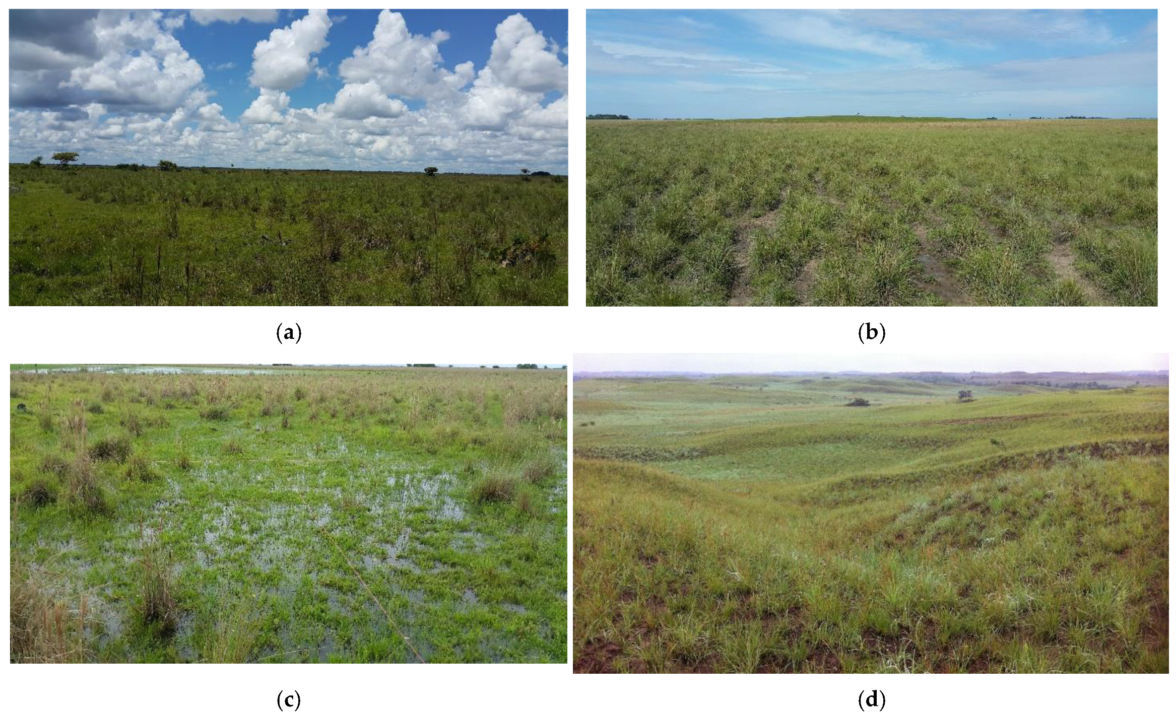

Disclaimer/Publisher’s Note: The statements, opinions and data contained in all publications are solely those of the individual author(s) and contributor(s) and not of MDPI and/or the editor(s). MDPI and/or the editor(s) disclaim responsibility for any injury to people or property resulting from any ideas, methods, instructions or products referred to in the content. |
© 2024 by the authors. Licensee MDPI, Basel, Switzerland. This article is an open access article distributed under the terms and conditions of the Creative Commons Attribution (CC BY) license (https://creativecommons.org/licenses/by/4.0/).