1. Introduction
This study focuses on finding an assessing methodology to quantify the impacts of filtering techniques on the spatial reliability of the social media data (SMD) to acquire the most suitable, reliable, and accurate SMD based on the subject for using it in various approaches. Contextual errors at the filtering stage of dealing with SMD result in focusing on irrelevant events, irrelevant reactions, and irrelevant locations with regard to the event. These errors result in the creation of unreliable or inaccurate maps relating to the event—what we will refer to as the domain in this study. Many studies have examined the reliability of SMD, mostly those that are found on Twitter [
1,
2,
3]. The Twitter platform is selected as the SMD resource for this study due to its geotagging options and wide usage throughout the world [
4].
Social media has diverse topic content sourced by human sensors [
5,
6,
7]. However, it does not provide a direct motivation to contribute to data production apart from the existence of a number of volunteer-based data gathering platforms [
8,
9,
10]. This makes social media analysis different from the analysis of structured data. Therefore, there is a need to filter such data to retrieve the relevant data for a selected domain.
For coarse-grained hot topic analysis, for example, if there has been a terror event in a city, non-relevant outliers might easily be filtered out from streaming data by using density-based clustering approaches [
11,
12]. Conversely, fine-grained filtering can robustly discretize noisy content for fine-grained analysis [
13]. For instance, incidence mapping during and following a terror event and the fine removal of discrepancies by fine-grained filtering help to produce more reliable maps to detect the location and the impact of the event. This, in turn, can support coordinated and accurate responses and the management of the emergency in question.
The terms accuracy, reliability, and credibility are generally used to evaluate the quality of SMD. The relationship between spatial information extraction and the truth in social media analyses is defined as its accuracy by [
14,
15,
16,
17,
18]. These studies used the concept of accuracy for the estimation of the living, working, or traveling locations of the users based on their social media feeds by using the distance between the geotagged and actual locations. The distance used in these studies is the Euclidean distance, that is, the distance between two points either on a flat plane or the 3D space length that connects two points directly using Pythagoras’ theorem [
19]. The concept of reliability mostly focuses on the internal accuracy of the data itself, or the method that is used to process the data as mentioned by Lawrence [
20]. This involves the investigation of the relationship between two different sentiment analyses’ statistical scores. Credibility is a term for the accountability of the source of the news in the new and traditional media. For social media credibility, this involves a consideration of the profile of the user, friendship networks, and the acts of the users such as tweets, retweets, likes, and comments, as suggested by Castillo Ocaranza et al. [
21]. Abbasi and Liu [
22] considered the credibility of social media by remarking on the activities of coordinated users that act together as a pack.
To date, there have been several studies on the credibility [
21,
22], accuracy [
14,
15,
16,
17,
18], and reliability [
20,
23,
24] of SMD, but those are somewhat limited because they have only focused on the results of the analyses, not on the filtering algorithms. However, most of the time, SMD are filtered based on the words and hashtags based on the event before they are analyzed [
25,
26,
27,
28]. Considering the negative nature of the disaster domain content, sentiment analysis can be seen as an approach that can be used to access related content from a wider perspective than that from the results of hashtag and bag of words filtering. Thus, focusing only on the SMD analysis results in ignoring the filtering techniques, thus misdirecting the assessments. Depending on the degrees of accuracy and reliability, which were referred to as aspects of the quality [
29] of the SMD filtering algorithm, the quality of the analyses changes.
There are two prominent approaches in the literature with regard to sentiment analysis [
23,
24,
30]. The first method utilizes a subjectivity lexicon, involving a glossary with sentiment scores or labels for each word or phrase. It involves scanning documents or phrases to determine the constituent total word score in terms of polarity. The second is a more statistical approach that exploits learning-based algorithms. However, it does not work well in the case of fine-grained phrases such as those found in social media content [
31]. In addition, statistical approaches might not work well on agglutinating and morphologically-rich languages such as Turkish, Korean, or Japanese [
32]. There have been several attempts to perform and test polarity analyses in the Turkish language, some of which are based on translating English subjective lexicons into Turkish [
33,
34], while others rely on classifiers across conceptual topics [
32] or rely on the linguistic context in Turkish [
35]. The use of sentiment analysis can vary according to the domain (e.g., specific topics such as disasters, opinion columns, or music) that it is used for. While the domain-independent lexicons provide fast and scalable approaches for general purposes, domain-based lexicons are valid across specific topics and cultures [
31]. In terms of the language used, the richness of the subjective lexicon is as important as the techniques and methodology selected. There are plenty of different lexicons for English with rich word content that quantify polarity by scoring [
30], by assigning several emotions to each term [
36,
37], by labelling terms as positive/neutral/negative [
38,
39], and by scoring each term’s polarity strength from minus to plus [
30]. On the other hand, most other languages, including Turkish, lack comprehensive subjective lexicons. However, to the best of our knowledge, there are a couple of lexicons for the Turkish language. Dehkhargani et al. [
31] generated a SentiTurkNet (STN) lexicon equivalent to the English translation of SentiWordNet [
38], while Ozturk and Ayvaz [
40] produced a Turkish lexicon consisting of over 5000 terms, determined as being terms found in frequent daily use, which are labelled as positive, negative, or neutral. This lexicon is entitled The Lexicon of Ozturk and Ayvaz (LOA) in this study. Previous studies of Turkish content involve domain-independent sentiment analysis, and the lexicon is mostly implemented over long texts. Hence, the performance of previous studies is unknown in terms of how they deal with short texts from social media with regard to a domain.
The novelty of this study is the development of a methodology for filtering the SMD based on relevance and spatial accuracy, by comparing the current techniques for filtering. Another outcome of this study is that we have developed a spatial similarity index to validate the spatial accuracy of the methodology along with the filtering techniques. The SMD of this study is acquired from two terror events that occurred in Istanbul. Consequently, the textual data of the tweets are in Turkish. Another distinction of this study is creating a methodology for a language that is not English. Most of the studies for the filtering and sentiment analyses of the tweets relate to the English language [
30,
41,
42]. It has been discovered that using these techniques without proper adjustments based on the event or language provides a very low rate of success for agglutinative languages like Turkish, due to the use of suffixes at the end of words and the large amounts of homonyms [
21,
31,
33]. As Castillo Ocaranza, Mendoza, and Poblete Labra [
21] indicate in their study, the filtering and ensuring the credibility of tweets in Spanish requires manual labeling, due to the possibility of non-relevant classifications.
Those type of situation with regard to filtering and language affect the accuracy and reliability of the resulting maps (event, hazard, or risk maps). Previous studies have mostly focused on where the event occurred geographically and how big it was, without considering the reliability of the fine-filtering techniques used or the impacts of filtering reliability on incidence mapping [
1,
2,
3]. However, the quality considered in this study is based on how correctly the SMD are filtered and how correctly these filtered data are reflected in the creation of maps, both spatially and sentimentally.
In this study, the domain selected is that of terror attacks. The events chosen were two such attacks in Istanbul in 2016, and the of all the tweets acquired in relation to these attacks were in Turkish. To investigate the effects of the filtering accuracy on the maps in geographical terms, the results of every filtering technique were mapped using a generic method. The determination of the accuracy of the filtered tweets involves the use of manually-labeled tweets as ground truth, such as by Gupta, Lamba, and Kumaraguru [
2] and Castillo Ocaranza, Mendoza, and Poblete Labra [
21] used in their research. Then, the maps associated with each filtering technique were analyzed in terms of the ground truth map.
At this stage of the study, various similarity indexing methods were used, and a new similarity index was introduced as the Giz Index. The Giz Index is designed to check the similarities of the values, sizes, and proximity of spatial objects, which were filtered and mapped using a technique involving the success percentages with respect to a ground truth map. The novelty of the newly developed similarity index is its ability to provide spatial intersection, proximity, and size together. For this reason, it can also be used for many studies to detect the spatial accuracy of the generated, estimated, simulated, or predicted maps with respect to the truth. Finally, the results from every similarity index method, including the newly developed Giz index, were compared with the ground truth map. The comparison showed the best combination of filtering technique and similarity indices to create event maps with regard to SMD. This study provides a methodology that can be used to accurately and reliably filter SMD and offers a method for investigating the effects of filtering techniques on map accuracy.
2. Materials and Methods
The methodology of this study began with an exploratory analysis of rough filtered Twitter data to create an approach for fine filtering domain-based data. In this way, noisy outliers not related to the domain could be discretized. To build up the approach for filtering out discrepancies using sentiment analysis and machine learning techniques, the basic workflow of data science [
43], which is import → tidy → understand (visualize → model → transform) → communicate, was followed, as shown in
Figure 1. Similarly, data processing is interpreted by considering the taxonomy of data science (obtain → scrub → explore → model → interpret) as suggested by Mason and Wiggins [
44].
Figure 1 presents the parts of the methodology, with the data import and retain part in white; the data tidying part as grey; the data exploration part in blue; the data processing part in green; and the data interpretation part in yellow, pink, and turquoise. Each part of the methodology is schematically extended with the use of figures (
Figure 2,
Figure 3,
Figure 4,
Figure 5,
Figure 6 and
Figure 7) and explained in the following subsections. With respect to this,
Section 2.1. provides a technique for geo-referencing data acquired from the Twitter stream by using Twitter API. This part is compiled with the use of Java as described in Gulnerman et al. [
45] as Geo Tweets Downloader (GTD). In
Section 2.2, the data tidying details are given in the order of pre-filtering, cleaning, and labelling to generate ground truth data. In
Section 2.3, data exploration techniques such as word clouds, comparison clouds, and dendrograms that are used for this study are explained. This exploration contributes to the development of the text pre-processing function that is part of the data tidying part. In
Section 2.4, the methodology of adapting the most common text classifying techniques to a terror domain-based filtering is introduced. In this part, two different sentiment lexicons for the Turkish language and three different machine-learning techniques are presented for automatically filtering relevant content. In
Section 2.5, the spatial interpretation methodology is introduced for precisely quantifying how textual filtering influences the spatial accuracy of the maps produced. This interpretation involves the following steps: 1—the production of a hotspot map for manually labelled relevant data (the ground truth map), 2—the production of hotspot maps for each filtering technique in terms of relevant outcomes (a predicted map), and 3—quantifying the similarity between the ground truth and predicted maps (spatial accuracy measure). In this similarity quantification process, current similarity indices (2.5.2) and a new similarity coefficient entitled the Giz Index (2.5.3.) are utilized for quantitatively interpreting the spatial accuracy of the maps produced. Features such as spatial proximity and spatial cluster size are taken into account by the Giz Index but not by the current indices. This is explained and compared with the test data in
Section 2.5.3 to prove that the proposed index performs better for the spatial interpretation.
2.1. Data Importing and Retaining
Geo Tweets Downloader (GTD) [
45,
46], a Java-based desktop program that allows filtering by the use of a spatial bounding box and omits non-geotagged tweets, was adopted to collect and spatially filter Turkish data. GTD utilizes Twitter APIs [
47,
48] that provide public status tweets in real-time. It also helps configuration with regard to the use of PostgreSQL in order to store retained geotagged data. By means of GTD, public status data are collected continuously up to the limits of the API usage. Since the tweets collected are of public status and geotagged, the number of tweets that were posted during the period under consideration was lower than normal. However, the aim and technique used do not need to capture all of the tweets posted to test the approach, which involves highly related filtering.
2.2. Data Tidying
Social media analysis with regard to an event starts with accessing the related data chunk. This is mostly obtained by querying the hashtags used, or probable keywords that are related to the domain. This tends to bring a mixture of data that is basically dominated by related content. However, it still includes noise in the form of non-relevant data. The first part of the data tidying process involves filtering the retained data using probable keywords for the disaster domain under consideration. Following this, the tweets generated by newsfeeds are discretized to avoid spam or non-individual posts. In the next part of data tidying, each tweet content is labeled as relevant, partially relevant, or non-relevant, in order to explore content commonalities and differences in the subsequent exploration part. Manual labeling is determined as follows:
Content related directly to a disaster event is marked as relevant;
Content related to a disaster in a general manner, such as criticism of a political party or memory of an old disaster event, is marked as partially relevant;
Content related to a very different context to a disaster event such as “I am like a bomb today” or “I am bored to death” is marked as non-relevant.
The grey line in
Figure 1 is extended in
Figure 2 to show the steps of the data flow for data tidying. Each step in
Figure 2 represents:
The acquired data table being produced;
Pre-filtering using domain-based keywords (rough filtering);
Newsfeed account removal from the data using media related keywords;
Manual labeling as relevant, partially relevant, or non-relevant to the domain;
Labels being appended to the data table.
This process provides pre-filtered and labeled data for the data exploration part. In this data tidying process, there is also a text-cleaning step, which is re-designed as a result of the outcomes of the data exploration. The tr_text_clean [
49] function is combined with the following steps:
The fixing of encoding problems due to different Turkish language characters;
The removal of emoticons, punctuation, whitespaces, numbers, Turkish and English stop words, long and short strings, and URLs.
This initial step eases the tokenization of each word as part of the next processes with regard to text mining. Cleaning steps were determined recursively according to the outcome of the data exploration part to find the best pre-processing steps for the language in this study. With respect to this, the text cleaning part was re-designed with the removal of language encoding problems and with a decision to keep the suffixes. This is because the suffixes vary in terms of pairing word to the relevancy class that is discovered in the bi-gram word clouds in the data exploration part. While this tidying step was utilized to regulate the text content for further processing, data still might have included numerous irregularities such as spelling errors, jargon, and slang that could decrease the performance of further processing.
2.3. Data Exploration
Explorative data mining methods were used to identify similarities and differences between relevant, partially relevant, and non-relevant chunks of manually labeled tweets. Commonality and comparison clouds, a pyramid plot, and word networks were visualized to gain insight into the data for further processing.
The blue line in
Figure 1 is extended in
Figure 3 to show the data flow steps for data exploration purposes. Each step in
Figure 3 represents:
Data division in terms of label type and the conversion of the data type from data frame to corpus;
Divided data assignment as corpus in terms of label type;
Text cleaning for each corpus using the tr_text_clean function;
Uni-gram Document Term Matrix (DTM) creation for each corpus (each term has a word);
Assignment of three DTMs for relevant, partially relevant, and non-relevant data;
Top 100 most frequent words determination in three DTMs;
Commonality cloud plot with varying word size in terms of word frequency;
Fifty most frequent distinct terms identification in relevant and partially relevant, and non-relevant DTMs;
The creation of a comparison cloud plot with the determined distinct terms in DTMs;
The creation of a word network based on hierarchical clustering;
The creation of a word dendrograms plot to reveal the term associations;
The calculation of the frequency percentage of commonly used terms in terms of relevant and partially relevant, and non-relevant DTMs;
The creation of pyramid plots with common terms in DTMs, ordered by the frequency percentage difference;
Bi-gram Document Term Matrix (DTM) creation for each corpus (each term has two words);
The assignment of three bi-gram DTMs for relevant, partially relevant, and non-relevant data;
Determination of the 100 most frequent bi-gram terms in relevant and partially relevant DTMs;
The creation of a commonality cloud plot with a varying plot size of bi-grams in terms of frequencies in DTMs;
The determination of the 100 most frequent bi-grams in non-relevant DTMs;
The creation of a commonality cloud plot with a varying plot size of bi-grams in terms of frequencies in DTMs.
These help to explore relevant, partially relevant, and non-relevant data contents. The working details of the packages used in this data exploration process are given in the following subsections. During this exploration, the importance of suffixes for discrimination in terms of relevance and the word association differences in terms of relevancy were explored. With respect to this, word stemming was not applied in the text cleaning function, and the deficit in terms of the use of unigram pre-filtering was revealed.
2.3.1. Commonality Cloud
This function is deployed as part of the “wordcloud” package [
50] in R, runs over a term’s frequency, and plots the most frequent “n” number of terms (words) as determined in the function argument. For this study, the top 100 terms were plotted to show which terms have dominance within the dataset.
2.3.2. Comparison Cloud
As with the commonality cloud, this function is also deployed as part of the “wordcloud” package [
50]. For a comparison cloud, two chunks of data are required in order to be able to compare the most frequently used terms. In this work, it was used to see which common words were most frequent in both labelled datasets. This function provides insights for sentiment analysis that depends on constituent word scoring without any weights.
2.3.3. Pyramid Plot
This function is deployed within the “plotrix” package [
51] and is used to show frequency differences in both chunks. Frequency difference is normalized with the division of the maximum term frequency in datasets, and ordered in terms of the differences. In this study, the use of a pyramid plot visualized 50 words in the datasets that have the highest rates of difference from each other. This plot was utilized to express the weights of terms that could be used for the intended classifier.
2.3.4. Word Dendrogram
The “dist” and “hclust” function from the “stats” package [
52] was utilized to create a word network as a hierarchical cluster, and the “dendextend” [
53] package was adopted to visualize and highlight terms in a dendrogram. The Euclidean method was used in the arguments of the “dist” function to determine the distance between terms before the hierarchical cluster process. The dendrograms of relevant, partially relevant, and non-relevant sets of data were expressed to determine word association differences.
2.4. Data Processing
Considering the insight gained from the data exploration part of the methodology, the processing part was carried out using the different filtering techniques based on sentiment lexicons and machine learning. In the first three techniques, the current generic subjective lexicons for the Turkish language [
31,
40] were exploited to classify a roughly-filtered dataset as being relevant, partially relevant, or non-relevant. The fourth and fifth techniques used the manually labelled data to allow building a machine learning classifier for fine-grained filters.
A domain-based perspective was built by exploiting previous similar cases. The use of subjectivity lexicons to filter out non-relevant content and for proposing a way of dealing with terror domain-based data with regard to the Turkish language was a brand-new approach in terms of SMD analysis. Subjectivity lexicons were used to avoid any misunderstandings with regard to Turkish words. For example, the word “bomb” can be used to describe the detonation of an explosive instrument or as the name of a popular dessert in Turkey. This is why valuable information from the posts was not ignored; only relevant classifications were targeted by using the subjectivity lexicons to pick out the relevant homonymous words in the Turkish language. However, it clarifies the benefits of the use of word suffixes (i.e., without stemming a word) in Turkish.
From this first perspective, all relevant content was supposed to include negative sentiments, while the non-relevant contents were considered to be positive. The first generic lexicon comprehensively developed for Turkish is STN [
31], which has nearly 15,000 terms (uni /bi-gram). STN provides the term’s sentiment scores (from 0 to 1) for each sentiment label (positive, negative, and objective), and the winning sentiment label for each term. In this study, the first technique scanned the constituent words of tweets regarding the sentiment labels for each term, and the content of each tweet was classified in terms of the highest count of the sentiment labels.
As far as the second technique was concerned, the scores of each sentiment label as derived from STN were taken into consideration, and the scanned terms for each tweet were summed to find out the most weighted sentiment relating to that content. The highest scored label classified the tweet content as being relevant for the highest negative, partially relevant for the highest objective, and non-relevant for the highest positive.
The third technique used another lexicon for the Turkish language (LOA) created by Ozturk and Ayvaz [
40], which depends on over 5000 commonly-used daily words scored from -5 to +5 by three people. The average of these three was accepted as the polarity score for each term. For the third technique, tweets were scanned to match the terms in the LOA, and the scores of the matched words were summed to classify the contents, with a minus score identified as being relevant, a zero score as being partially relevant, and a positive score as being non-relevant.
There are few studies on comparisons between the text filtering of SMD [
54,
55,
56,
57] because most of the machine learning techniques are not considered for SMD. As can be seen from those studies, the most common and efficient techniques that can be used with regard to text filtering are Naive Bayes, Neural Network, and Support Vector Machine [
58,
59,
60,
61]. That is why these three techniques were considered in this study to filter domain-based SMD.
For the fourth technique, a machine-learning perspective was used to create a classifier. The Naïve Bayes (NB) classifier [
62] was utilized, based on the probabilistic determination method. According to this method, a classifier considers the likelihood probability of each class over a trained dataset. It then calculates the conditional probability of each term seen in the trained dataset regarding each class. The classifier performs this analysis over the test data by multiplying the probability for each term scanned for each tweet, as well as multiplying the likelihood probability of each class. Finally, the classifier compares the probabilities of each class and picks the highest one to label. The method considers the rate of incidence for the commonly-used words in each class. This is advantageous in terms of classification performance with regard to roughly filtered data.
In the fifth technique, the Neural Network (NN) classifiers were trained. The ‘nnet’ package [
63] was utilized to model the classifiers. In terms of the NN principles, for training a dataset, a document term matrix (DTM) is accepted as input signals with class labels. Three classifiers are trained using a multi-class dataset. The weights of hidden layers are not initiated up front, and training is performed with 500 iterations. Considering text classification with DTM is not a linearly-separable problem, and it does need hidden layers when classifying with an NN classifier. Therefore, the hidden layer parameter in the classifier is specified as 1, 2, and 3 to experimentally determine the best hidden layer number. Increasing the hidden layer number provides high classification accuracy, but also creates a time cost. However, the main aim of the study was not finding the best fit for a NN, but assessing ways to determine the outcomes of faster filtering techniques when mapping. With respect to this, the NN classifier that showed a reliable statistical performance with two hidden layers was accepted in this NN processing part.
In the data processing part, sentiment lexicons and machine learning techniques were mainly used to filter domain-based data. The sentiment lexicons used were the ones for use with the Turkish language. The machine learning techniques used were the ones commonly used for text classification [
58,
59,
60,
61]. In addition to the NB and NN, Support Vector Machine (SVM) is another popular technique used for text classification. As the sixth technique, an SVM classifier was trained. The ’e1071’ package [
64] which is one of the Misc Functions of the Department of Statistics, TU Wien, was utilized to implement the classifier. The package allows the training of an SVM classifier by vectorizing each term count in each document with the training labels. Since SVM provides successful results for linearly-separable problems, different kernels such as polynomial, radial, and sigmoid were used for the SVM classifiers. Although the SVM classifiers achieved a high degree of accuracy due to the use of unbalanced datasets in this study, they achieved zero sensitive results for two of the three classes. Therefore, it was decided that SVM was not suitable for further assessment in this study.
The green line in
Figure 1 is extended in
Figure 4 to show the data flow steps for data processing. Each step in
Figure 4 represents:
Data division into event day data and training data;
The conversion of the data type from data frame to corpus for event day data;
Data assignment as corpus for event data;
Text cleaning for event corpus using the tr_text_clean function;
Uni-gram Document Term Matrix (DTM) creation for the cleaned corpus;
sentiTurkNet polarity lexicon data frame creation;
The creation of inner joining terms in event data DTM and terms in sentiTurkNet;
The aggregation of negative values, objective values, and positive values for terms in each document;
Polarity decisions for each document depending on the biggest values of each aggregation;
The appending of polarity labels to event data;
The assignment of event data with the polarity labels as STN_byScore data;
The counting of the negative (−1), objective (0), and positive (1) labels of terms in each document;
Polarity decision making for each document, depending on the biggest counts;
The appending of polarity labels to event data;
The assignment of event data with the polarity labels as STN_byLabel data;
LOA polarity lexicon data frame creation;
The inner joining of terms in event data DTM and terms in LOA;
The aggregation of polarity scores of terms in each document;
The determination of polarity labels based on the sign (−, +) of polarity score aggregation;
The appending of polarity labels to event data;
The assignment of event data with the polarity labels as LOA data;
The conversion of the data type from data frame to corpus for the training data;
Data assignment as corpus for the training data;
Text cleaning for the training corpus with the tr_text_clean function;
Uni-gram Document Term Matrix (DTM) creation for the cleaned training corpus;
The modeling of a naïve Bayes classifier with the training DTM;
The prediction of event DTM relevance with the naïve Bayes classifier;
The appending of a prediction label to event data;
The assignment of event data with the prediction labels as NB_pred data;
The modelling a neural network classifier with the training DTM;
The prediction of event DTM relevance with the neural network classifier;
The appending of prediction labels to event data;
The assignment of event data with the prediction labels as NNET data.
This provides us with classified event data as a result of the five different techniques. The classified data, in terms of different techniques, is further processed with the methodology given in
Section 2.5 for quantifying the impact of filtering on spatial accuracy.
If the language is different to the language of this study, the users should alter several steps shown within the methodology. In the data tidying step, data should be fixed due to encoding problems caused by different Turkish language characters. This tidying operation is specific to the Turkish language and should be changed for other languages that have different encodings. In addition to that, the stop word removal of the text cleaning part should be changed into the defined language if the language is different from Turkish. Another alteration in the tidying part might be the addition of the “stemming” process. This study omitted the “stemming” since the suffixes contribute to the discrimination of the relevance as discovered in the data exploration part. However, the “stemming” operation could contribute to the discovery of highly related content in other languages. In the data processing part, the sentiment lexicons are the ones for Turkish Language, and these also need to be changed if the filtering process will be carried out with the sentiment lexicons of a different language.
The domain in this study is defined as the terror attacks and this should certainly contain negative sentiment. As was also discovered in the data exploration part, irrelevant data contain positive sentiments. That is why the use of sentiment lexicons can be successful for this terror domain. That means that sentiment lexicon use should be avoided for determining the relevancy of domains that can contain all types of sentiments. For instance, in marketing research, the domain may include positive, neutral, or negative sentiments; therefore, the use of sentiment lexicons is not plausible for filtering relevant data.
2.5. Interpretation of Spatial SMD
Accurate text mining for fine filtering is the first aspect associated with producing more reliable maps for domain-based SMD analyses. However, on its own, it is not enough to determine the spatial accuracy of the maps produced from the SMD. To determine how different filtering techniques impact on spatial accuracy, this study proposes a spatial interpretation method. The interpretation method involves two main steps—spatial clustering and spatial similarity calculation. In
Section 2.5.1, the details of the spatial clustering are given for incidence mapping the filtered data that is used for this study. In
Section 2.5.2, the current coefficients for the spatial similarity calculation are introduced. In
Section 2.5.3, the new spatial similarity coefficient entitled the Giz Index is proposed with quantitative comparisons of the previously-introduced indices over designed test data. The similarity scores vary in terms of the chosen similarity coefficients. Therefore, it is important to determine which spatial similarity index is used. In
Section 2.5.3, a test designed for the comparisons of similarity indices is used to reveal which index returns a plausible similarity value for incidence map comparisons.
2.5.1. Spatial Clustering
There are a number of spatial clustering algorithms [
65] and methods used for spatial event detection, whose results vary in terms of algorithm selection and methodologies [
12]. Considering the conflicts between different clustering techniques and pre-specified parameters (such as the number of the clusters and required minimum number for each cluster), the Getis-Ord spatial clustering algorithm [
66,
67] is chosen for each dataset to compare spatial variances due to the different filtering methodologies applied previously. While performing Optimized Hotspot Analysis located in the Spatial Statistics toolbox in ArcMap [
68], the cell size is defined as 500 meters in terms of street-level resolution [
69], as it is intended to be fine-grained, and the aggregation method is determined as a hexagon polygon to allow us to use the connectivity capacity of a clustering lattice shape [
70]. This first step provides Hotspot maps for different filtering methodologies, which serve as base maps for the next step—spatial similarity calculation.
The hotspot mapping details of the filtered data are given by the yellow line part in
Figure 5. Each step in
Figure 5 represents:
Filtering data in terms of day of the event;
Relevant data selection in terms of manually labeled data;
The production of a hotspot map for manually filtered relevant data;
The assignment of the manually filtered data hotspot map as the ground truth map (T);
Relevant data selections in terms of each automatically classified dataset;
The production of hotspot maps for each automatically filtered relevant dataset;
The assignments of the automatically filtered data hotspot maps as filtered maps (F1-5).
This provides ground truth and filtered data hotspot maps for the spatial similarity calculation described in the next subsection.
2.5.2. Spatial Similarity Calculation
In various fields such as biology [
71,
72], ecology [
73], and image retrieval [
74], numerous similarity indices have been proposed. Choi et al. [
75] present an extensive survey of over 70 similarity measures in terms of positive and negative matches and mismatches when it comes to comparisons. Similarity measures are also in use and vary for the comparison between two maps in order to find semantic similarities between land use, land cover classifications, temporal change, and hotspot map overlaps [
76,
77,
78]. In this study, the similarity between incidence maps is tested with the use of similarity coefficients. Incidence mapping similarity is a special case for the similarity measures since the incidences cover a small proportion of the pre-defined area (such as a city, a region, or a district). Therefore, the negative matches within the observed area should be disregarded in order to avoid a high degree of misleading similarity due to the high cover of negative matches. Arnesson and Lewenhagen [
78] propose the use of four different quantitative similarity measures for determining the similarities or differences between hotspot maps. These are the Jaccard Index (1) [
79], the Sorensen-Dice Index (2) [
80,
81], the Kulczynski Index (3) [
82], and the Ochai Index (4) [
72], each of which are utilized for similarity calculations. These measures return a similarity score of between 0 and 1 regarding True-True (a), True-False (b), and False-True (c) hotspot counts in a comparison between truth and prediction spots. These indices disregard negative matches (False-False (d)) [
72,
78] that are the first requirement for incidence mapping similarity calculations. However, these indices are not specifically designed for spatial purposes, given that they disregard the proximity between mismatching hotspots and the positive matches. In this respect, a new spatial similarity index is formulated for quantifying incidence mapping reliability with regard to the ground truth data.
Similarity index calculation details are given in the pink line in
Figure 5. Each step in the pink line represents:
This provides the four spatial reliability scores in terms of current similarity measures. However, the applicability of the measures is uncertain with regard to the incidence mapping, since the measures do not consider the proximity of the non-intersection areas, even if they are neighboring. That is why the Giz Index is proposed as a spatial similarity index for incidence mapping studies. In the next subsection, the Giz Index is formulated, and a comparison test between indices is provided over test data. This comparison is provided to explain the eligibility of the Giz Index for incidence mapping comparisons, while the others are not appropriate for every circumstance.
2.5.3. Giz Index
In a spatial context, omitting negative matches allows a more specified representation of hotspot similarities between two maps. Otherwise, the results might be dominated by negative matches and return over 99% similarity for almost all comparisons. However, the use of coefficients for spatial purposes has some weaknesses, such as disregarding the size of separate clusters and the proximity between non-intersecting clusters. The claim here depends on Tobler’s First Law of Geography, “everything is related to everything else, but near things are more related than distant things”. Thus, the distance and the size of each cluster needs to be considered in order to draw an accurate spatial similarity index regarding proximate things that might influence each other. A new spatial similarity index has been developed to represent to extent to which two maps are approximately similar to each other. This is entitled the Giz Index. This index is referred to within the formulas and figures as GI. This index considers each hotspot cluster in the first map as truth (c1..n) and in the second map as prediction (k1..n).
The methodology of the index detects the area of each cluster (A
c1..n, k1..n), and considers whether they are intersecting to form an area of intersection (AI
c1-k1) or non-intersecting to form a residual area of intersection (ANI
c1-k1) and the distance between clusters (D
c1-k1). The Giz Index is formulated as in Equation (5) for single cluster similarity.
In the first part, the equation handles the similarity of intersecting areas (AI). AI similarity is obtained by dividing intersecting areas (AIc1-k1) of the cluster (Ac1) and multiplying them by the normalized distance between clusters (ground truth and prediction). This normalized distance is taken as 1 for the intersecting areas part, and is always less than 1 for a non-intersecting area. At the same time, as the distance increases between clusters (c1–k1), the normalized distance will decrease relative to the square root of the cluster area. In the second part, non-intersecting part similarity is calculated with the very same formula as in the first part. There is a condition based on the sizes of the Ac1 and ANIc1-k1, where the area ratio in the second part of the formula is reversed. For instance, if the area of the first cluster (c1) is 4 units, and the non-intersecting part is 10 units, the ratio is reversed to become 4/10 instead of 10/4.
The Giz Index calculation details are given by the turquoise line in
Figure 6. Each step in
Figure 6 represents:
The variables’ calculation for each comparison (similarity calculation) for the Giz Index:
c1..x = dissolve(T) (determination of clusters for the truth map by merging adjacent hexagons);
Ac..x = area(c1..x) (defining the area of each cluster in the truth map);
k1..x = dissolve(Fx) (determination of clusters for the filtered map by merging adjacent hexagons);
Ak..x = area(k1..x) (defining area of each cluster in the filtered map);
Dcx-kx = (distance(centroid(c1..x),(centroid(k1..x))) (defining distance between each truth map cluster and each filtered map cluster); this step is important in order to define which cluster in the filtered map is compared to which truth map cluster, and the closest distance determines the candidate cluster in the truth map;
AIcx-kx = intersect(cx, kx) (defining the area of the intersecting clusters);
ANIcx-kx = extract(kx, cx) (defining the area of non-intersecting cluster parts);
The calculation of similarity between truth maps and filtered maps using the Giz Index according to Equation (5).
This provides similarity measures weighting the degree of similarity depending on the proximity between truth map clusters and filtered map clusters.
The Giz Index is tested and compared with the current indices with regard to the test data that are displayed in
Figure 7. The test data include six instances, and each instance has two predictions (p1, p2) and one truth cluster. The test data are developed to reveal the response details of the similarity indices in terms of the different sizes of prediction clusters and the distances between the prediction cluster and the truth cluster.
The similarity between the prediction clusters (p1, p2) and the truth cluster for each instance is calculated using the current indices and the proposed Giz Index. The similarity results vary between 0 and 1 and are presented in
Table 1. In the first three instances, there are no intersecting clusters. Therefore, the results of the current indices return a 0 value; the prediction is either proximate to or far from the truth cluster. Additionally, these indices disregard the non-intersecting cluster size in these zero intersection circumstances. On the other hand, the Giz Index returns varying similarity values in terms of the proximity and size of the non-intersecting clusters— in these instances I, II, and III. When the differences in size and distance are higher, the Giz Index (GI) is closer to 0; otherwise, it is closer to 1. The scores of the current similarity indices respond to the size of the intersecting area in instances IV, V, and VI. When the intersection is proportionally higher, the current scores become higher, as in the GI. However, the residual area of the cluster has zero addition to the similarity increase even if they are placed in neighboring parts of the truth cluster. In respect to the results, it is obvious that the current similarity indices totally disregard non-intersecting parts when there is no intersecting cluster. Therefore, the current indices might cause misinterpretations in incidence mapping studies, since the near incidences to the real incidence areas have value when it comes to determining the exact incidence area. In other words, the occurrence of close incidences on a map can be interpreted as signs indicating the main event. Therefore, the proximity of non-intersecting clusters and size should be considered for the correct interpretation of the maps.
The Giz Index supports exploratory inferences when the quantitative measure is between 0 and 1, by considering both the size of spatial clusters and their proximity. The size and location accuracy are important for the several subjects that form the domains, and the Giz Index can provide a quick and automatic spatial interpretation of the analyzed data. This index can also be used for a quick look at the validation processes with regard to social media data if there are any other secondary data sources that can be accepted as the truth. The Giz Index can also be used for various domains such as concerts, elections, and marketing, in addition to disasters, as mentioned in this study. The spatial similarity introduced in this research can be used for the spatial comparison of simulation maps and estimation maps, and the resulting maps associated with different studies using different methodologies can be used for similar purposes.
3. Case Study
3.1. Importing and Retaining Data
In this study, 8 months of data from May to December 2016 were selected regarding 10 terrorist attacks that occurred in Turkey. During that period, geo-referenced tweets were captured and inserted in the PostgreSQL database using GTD.
3.2. Data Tidying
Pre-filtering was done roughly using keywords such as “attack” (saldırı in Turkish), “bomb” (bomba in Turkish), and “explosion” (patlama in Turkish) to provide targeted chunks of data with a mix of relevant and non-relevant content. While filtering, all combinations of case-sensitive and Turkish character encodings were considered in order to retrieve all possible related content such as “saldırı”, “SALDIRI”, “Saldiri”, etc.
Following this, 285 tweets from six newsfeed accounts were detected and removed from the pre-filtered data due to possible content being mixed with diverse and non-relevant news. After removal, a total of 4395 tweets were classified manually using three labels: 1—relevant (RL), pertaining to newly-occurred terror attacks; 2—partially relevant (PR), related content including terror in general such as political party criticism or memories of an old terror event; and 3—non-relevant (IR), contents totally unrelated to a terror attack, such as “I love bomb dessert” or “Go team go, attack and beat them”. As labelled, 934 of the tweets were non-relevant, 799 were partially relevant, and 2662 tweets were directly relevant to a terror event. Maps of each set of IR, PR, and RL tweets were created and classified by month (
Figure 8).
One of the inferences while labelling is that social media users react to newly-occurring terror attacks by protesting about terrorists, the security services, the government, and political parties. However, many of the tweets include condolences to the families of the victims regarding second-hand information obtained from somewhere else such as traditional/news media. Very few of the users were sharing information about witnessing the incidents. Consequently, these inferences predominantly indicate a repetition of similar content. Thus, it can be said that mining for first-hand information is just like looking for a needle in a haystack. This first-hand information is of great importance for incidence mapping during or shortly after a disaster, as implied in the motivation for this study.
Prior to explorative data analysis, the text of the tweets was cleaned to avoid later problems when it came to processing a better bag of words. Therefore, emoticons, punctuation, stop words in Turkish [
83] and English, numbers, and URLs were removed from the tweets, and all encoding and letter case problems were fixed. In addition, city and county names with regard to Turkey that may create a bias in terms of this work, and were not needed while classifying content, were removed from the texts. Stemming, which is one of the further text cleaning steps, was ignored in this study. In this way, the aim was to preserve rich meaning differences with suffixes in Turkish. By using the tr_text_clean function, text cleaning of this work was undertaken on the one hand by including several functions from the TM package [
84] and the ggrepel package [
85] and, on the other, self-defined sub-functions. Details of the tr_text_clean cleaning function can be found in [
49] in terms of its use in similar works.
3.3. Data Exploration
Data exploration for Turkish terror domain-based data was handled descriptively using commonality and comparison clouds, a pyramid plot and a word dendrogram in order to show differences between terms (words) with regard to data relevant to the domain.
Commonality for uni/ bi-grams and comparison clouds are visualized (
Figure 9) after the several cleaning functions are applied to all three chunks of data. The commonality cloud plotted for uni-gram (a) represents the most frequent terms over all the labelled chunks, in which the relevant chunk dominates the frequency due to the relatively high number of tweets compared with other chunks. This means that hot topics dealt with during the disaster could be easily estimated by the use of the commonality cloud over the roughly-filtered data. The comparison cloud (b) displays the most frequent terms in both chunks, in terms of relevant/ partially relevant tweets and non-relevant tweets. The comparison cloud provides a more detailed explorative look by plotting frequent terms regarding non-relevant and relevant (partially or totally) chunks of data (b). Terms in this study are in Turkish and translated into English, with the words in parenthesis being the actual Turkish words encountered in this study. The first inference is that chunks include common terms such as ‘bomb’ (bomba), ‘explosion’ (patlama) and ‘attack’ (saldırı); dissimilar frequent terms include words such as ‘dessert’ (tatlı), ‘energetic’ (enerji), ‘mercy’ (rahmet)). The second inference is that some of the most common words in the comparison cloud have taken different suffixes. For instance, ‘attack’ in the relevant chunk has noun suffixes, while in the non-relevant chunk it is mostly used as a verb in the imperative mood. Therefore, these were assessed as different terms by omitting stemming in the pre-processing period.
In addition to the unigram word cloud, bi-gram word clouds are plotted for both chunks, whether the use of any bi-gram could be pervasive in either one or both (
Figure 9c,d). For instance, ‘God’s mercy’ (allahtan rahmet) is the most frequent bi-gram in the relevant (partially or totally) chunk, while ‘coming like a bomb’ (bomba geliyoruz) is the most frequent bi-gram in the non-relevant chunk. From the perspective of the subjective lexicons, we might consider that ‘God’ can be labelled as positive. However, in conjunction with ‘mercy’ it turns into a condolence phrase that has a negative sentiment. In the same vein, ‘bomb’ can be perceived as being negative or positive, while on the other hand ‘coming like’ expresses a positive sentiment, with ‘attack’ indicating negative sentiments. Those words are not ‘negators’ that directly invert a polarized meaning like the ‘not’ effect over adjectives, as in ‘good’ and ‘not good’. It shows the importance of word association in order to identify the correct sentiment.
A word dendrogram for each chunk is visualized to compare the changing word association between chunks. There are a couple of inferences from the dendrograms. The first one is that there are few branches for the same words with different suffixes in the same dendrogram, and also in different ones (such as; terör, terörü, teröre and terörsüz etc. colored as red in
Figure 10). These suffixes provide a clue about the other parts of the sentence. For example, ‘terror’ (teröre) could be completed with ‘damn’ (lanet) to create ‘damn terror’. Similarly, while the word ‘terörsüz’ means ‘without terror’, it could be completed with terms such as ‘wishing for a day without terror’ (colored as blue in
Figure 10). In addition, the word for ‘explosion’ (patlama) in a relevant dataset, is not directly associated with any word, while in the non-relevant chunk it is associated with ‘good morning’ (günaydın), ‘energy’ (enerji) and sampled as ‘Good morning! I have had an energy explosion today’ (colored as orange in
Figure 10). Furthermore, the leaves of dendrograms display commonly-associated words such as ‘wish’ ‘speedy’ ‘recovery’ ‘to the wounded’ (‘diliyorum’, ‘acil’, ‘şifalar’, ‘yaralılara’) in a relevant dendrogram, ‘counter’ (‘mücadele’ in Turkish), ‘terrorism’ (‘terörle’), ‘branch’ (‘şube’), ‘directory’ (‘müdürlüğü’) in partially relevant tweets, and ‘ready’ (‘hazır’), ‘to explode’ (‘patlamaya’) in non-relevant sets (colored as green in
Figure 10). Therefore, keeping suffixes is important, as well as assessing word associations in the same document to determine the exact sentiment.
The use of a pyramid plot also offers another chance to explore the (dis)similarity in terms of frequency between RL-PR and IR. The terms (“terör” in RL-PR, “bomba” in IR) that have the maximum frequencies in both chunks are assumed to be 100 units, and the frequency values of the other terms are normalized using a rate ratio, according to Equation (6). Normalization is applied to the RL/ PR and IR chunks separately in order to avoid the dominance of different chunk sizes.
The pyramid plot used in this study plots 50 common terms that have the highest frequency difference between the RL/PR and IR chunks, ordered by the normalized term frequency value difference (ntfv) (
Figure 11a) and ordered by the ntfv of the RL/PR chunk (
Figure 11b). This plot is important in that it shows that although there are common words, each has a different frequency rate in the various chunks. For instance, keywords such as “terör”, “bomba”, and “patlama”, used for rough filtering, are unsurprisingly placed at the bottom of the plot as the highest ntfv for the RL/ PR chunk, while they have 2.6, 100, and 9.6 ntfv, respectively, for the IR chunk. In addition, the plot provides the feasibility of looking more closely at the ntfv with regard to the same words with different suffixes, as in “terör”, “terrorist”, “terörü”, “bomba”, “bombalar”, “bombas”, and “bombayı”.
3.4. Processing Data
The explored data were processed using two lexicon libraries (STN and LOA) with three different processes (score, score label, and polarity labels) in order to determine the best fine-grained filtering process and its performance. In general, the terror domain filtering capabilities of current Turkish subjectivity lexicons were revealed before the implementation of the techniques with regard to two cases from the terror domain. As a result, all self-labelled data were processed with the current subjectivity lexicons in the form of STN and LOA. This resulted in the prediction of each tweet’s sentiments by separately utilizing terms with scores in STN, polarity labels in STN, and scores in LOA. To determine the content of each tweet—whether negative, positive, or objective—each tweet’s constituent terms’ label counts and score sums were calculated. The relevant metric for this score was chosen in terms of its overall accuracy according to Equation (7), which is the ratio of the correctly classified cases vs. the total data count.
These three processes respectively indicate that 36%, 40%, and 49% of the results are accurate for filtering. However, the first two STN processes resulted in 37% being non-applicable (NA), and the last process (LOA) resulted in 5% being non-applicable (NA) (
Table 2a–c). Thus, a 37% NA result can be interpreted as being inadequate in terms of the STN for the terror domain, while the LOA has a wider capability to cover terms with just 5% NA results. This might indicate that the LOA has more words that intersect with the domain terms. On the other hand, the overall accuracy for both lexicons is not sufficiently adapted to that domain to allow fine-grained filtering.
The explored dataset included tweets pertaining to several terror attacks that had occurred in Turkey. Two cases were picked for a comparison of filtering techniques and mapping reliability. In the first case, the test data were roughly-filtered data generated after the terror attack that occurred near the Besiktas Vodafone Arena (BVA) in the Besiktas district of Istanbul. The second case data were roughly filtered after the Ataturk airport terror attack (ATA). These two terror attacks caused many casualties and fatalities and created a threat to thousands of people in the urban area. Many people expressed their sorrow, offered condolences, and expressed their hatred of the attacks. Therefore, sentiment analysis was seen as a way of undertaking fine-grained filtering. Both datasets were processed with regard to the three lexicons and two machine learning-based techniques. The first three techniques were applied regarding each case of datasets. However, these processes returned some unlabeled outputs (NA), which were disregarded for the calculation in terms of accuracy. The confusion matrices of the first set of techniques are displayed in
Table 3a–c for the BVA and
Table 4a–c for the ATA. With regard to the fourth process, a Naïve Bayes classifier was trained and tested for the same events. The rest of the roughly-filtered and labelled data were used as a training dataset to build a Naïve Bayes classifier. As a result of this process, the classifier labelled all data with 87% accuracy (
Table 3d). This approach was tested with the second dataset generated after the ATA. The ATA event resulted in 84% accuracy (
Table 3d) using the same approach. The fifth process was a neural network (NN) classifier, which was trained using the manually labelled data. The model classified BVA and ATA data with 61% and 70% accuracy (
Table 4d,e), respectively. A hidden layer parameter was assigned as 1, 2, and 3 in order to find the best model for NN. In the NN processing part, an NN structure consisting of two hidden layers was adopted due to its reliable statistical performance.
A confusion matrix was plotted for the evaluation of each filtering technique with overall accuracy, sensitivity (recall), specificity, PosPredValue (precision), F1, F2, and G-Mean (geometric mean) scores. These scores represent details of the filtering performance. While accuracy indicates the general performance of the filtering process, it is not adequate on its own in some circumstances, e.g., a misleading high accuracy score can be seen for the unbalanced data classes due to zero sensitivity on all classes other than the major class [
86]. Data that were used in this study are unbalanced for the relevant (R) class, since the pre-filtering was applied for the day of the terror attacks. Although the classifiers were modelled to classify multi-classes, it is more important that the major class (R) is classified. In this circumstance, sensitivity, F1, and G-Mean metrics were proposed by the studies dealing with such data and classifiers [
86,
87,
88].
There are several inferences depending on the results listed in
Table 3 and
Table 4. The first one is that the Naïve Bayes classifier performance over two datasets is clearly better than that of the other four techniques in terms of the overall accuracy and sensitivity, F1, and G-Mean for the relevant (R) class. The performance ranking across both datasets is the same in terms of overall accuracy, which is NB, NN, LOA, STN by score, and STN by polarity label from the highest to the lowest. The rank is slightly different—which is NB, LOA, NN, STN by score, and STN by polarity label for BVA—but is again similar for ATA in terms of the F1 score. It is NB, NN, STN by polarity label, STN by score, and LOA for both BVA and ATA in terms of the G-Mean score. In terms of all scores, the performance rankings are very similar for both datasets. This means that the filtering techniques are precise and independent of the data.
3.5. Spatial Interpretation over Fine-Filtered SMD
As noted above, this study explored the fine-grained content filtering used to produce more reliable maps for specific domains. Each textually filtered dataset was overviewed with the use of confusion matrices, and this part of the study considered the textual accuracy of the tweets that can be used for a disaster domain. However, the spatial accuracy of the tweets needs to be determined in order to provide full reliability in terms of the sentiments and the location of the tweets. To determine the spatial accuracy, this study compared the manually-labelled and automatically-filtered data in the spatial context. There are diverse spatial clustering algorithms [
65] and methods for spatial event detection. The results vary in terms of the algorithm selection and the methodologies used [
12]. Given the conflicts revealed using different clustering techniques and pre-specified parameters (such as the number of the clusters and required minimum number for each cluster), a Getis-Ord spatial clustering algorithm [
66,
67] was chosen for each dataset to compare spatial variances due to the different filtering methodologies applied previously.
While performing Optimized Hotspot Analysis using ArcMap [
68], the cell size was defined as 500 m. This represented the street-level resolution [
69] necessary to allow a fine-grained analysis. To use the connectivity capacity of a clustering lattice shape [
70], hexagon polygons were selected in the aggregation method. The borderline of the city of Istanbul—where both terror events occurred—was taken as the analysis boundary. The outcomes of the analysis gave an explorative method for identifying the differences or similarities between the filtering methods and manually-labelled data (
Figure 12a
1,b
1). Manually-labelled data hotspots for BVA (a
1) and ATA (b
1) are taken as ground truth without concerning the credibility of the data posted in social media. Explorative comparisons of hotspots could be assessed in terms of the similarity of cluster locations, cluster sizes, cluster numbers, and distances between clusters.
For the ATA event, LOA (a4) looked more similar to the truth map than all the others, while it was the second most accurate one in terms of filtering after the use of Naïve Bayes. Interestingly, when the cluster size was used, the clusters of Naïve Bayes filtering were several times larger than the ground truth. Even though, in terms of cluster location, Naïve Bayes filtering gives an accurate result—since it includes the base clusters inside—in terms of cluster size, the level of accuracy does not meet expectations, whereas Naïve Bayes filtering comes first in terms of filtering accuracy.
For the BVA event, both STN filtering hotspots were seen to be scattered to several distant locations, and STN by score (b2), LOA (b4), and Naïve Bayes (b5) filtering display a rather more similar clustering pattern with manually-labelled hotspots (b1). However, clusters generated by the data filtered with STN by polarity label (b3) present moderate convergence to the base clusters (b1).
The similarity rates of hotspots are listed for each event, based on their similarity indices (
Table 5). In respect of this, the results vary in terms of the chosen indices and, at some points, the results of other indices converge to the Giz Index. There are several inferences that can be made from this. The first one is that the Jaccard Index (JI) performs well when the intersection converges to the size of the hotspots in either the ground truth or the filtered maps (
Figure 12a
4,b
6). Secondly, since the Sorenson Index (SI) formulates the intersection as double weighted, it converges to the Giz Index when the intersection area is significantly high (
Figure 12a
5,a
6,b
3,b
4,b
5). Kulczynski designates the same importance to the intersection part ratio to either ground truth or filtered map, and converges to the Giz Index, with the intersection ratio being similar in both maps (
Figure 12b
2,b
4,b
5). Therefore, it does not converge with the Giz Index score when the intersection area is disproportionately distributed in the truth and filtered maps as shown in
Figure 12a
2,a
5. Additionally, the Ochai Index considers the intersection ratio exponentially to total hotspot areas in both the ground truth and the filtered maps (
Figure 12a
6,b
2,b
4,b
5). This exponential weight creates a bias in terms of the size of the intersection without bothering about the distance between the non-intersected areas. The Giz Index calculates the similarity score in terms of all the required aspects (cluster size, spatial proximity, spatial intersection area, and non-intersected area) for the comparison of incidence maps.
The similarity threshold is identified as 0.7 for the use of filtering and mapping techniques. With regard to this, STN by score (STNScrPred) has a threshold of more than 0.70 similarity according to the JI and KI, while for the LOA (LoaPred) it has a threshold of more than 0.90 according to JI, KI, OI, and GI for the BVA event (
Table 5a). For the ATA event, with the exception of NN, all hotspot map displays have a reasonable similarity according to diverse indices (
Table 5b).
However, the Giz Index is accepted as the most appropriate similarity index for this study as it embodies spatial similarity, unlike the Jaccard, Sorensen-Dice, Kulczynski, and Ochai Indices. The results of the Giz Index for both events support explorative inferences, with quantitative measures between 0 and 1, by considering both the size of spatial clusters and their proximity. This is because size and location accuracy are important for studies including spatial analyses, such as disaster management involving such an analysis. The index can provide quick and automatic spatial interpretation of the analyzed data. When it comes to the Giz Index, which allows us to evaluate the data spatially, it offers sufficient similarity for both the BVA events with LOA, and the ATA event with the LOA, STN by score, and Naïve Bayes techniques.
3.6. Outcomes
As previously mentioned, the proposed methodology of this study can also be used for different domains such as elections, natural disasters, and marketing. As an example, if the domain is an election, the following procedures can be applied to map the reactions of social media. The first step is to correctly filter the SMD. For this step, the user should select the keywords for the election event such as politics, party, parliament, deputy, names of the parties, names of the candidates, election, referendum, etc. Following this first step, the filtered SMD will include non-relevant or partially relevant tweets due to the use of homonyms and metaphors. To filter out the non-relevant and partially relevant tweets, depending on the number of available tweets, a training dataset should be spared and labeled manually as being relevant, non-relevant, and partially relevant. This step can be automatically done by using web platforms such as Kaggle and Mechanical Turk [
89,
90]. This manually or web-based labeled dataset is used to train a Naïve Bayes Classifier, and this classifier is used to fine-grain filter the SMD. After the automatic fine-grain filtering, the relevant resulting labeled data can be used to create hotspot maps of social media reaction, changes in reaction maps, and the thematic and spatial distributions of reactions by using the Getis-Ord* algorithm. This map can show most and least favorite candidates, parties, promises, and the complaints of the electors in different spatial regions.
Temporal reaction maps can be compared by using the Giz Index to evaluate differences in terms of the election campaign based on the candidates or parties. The reaction maps of the candidates or parties before and after meeting times can also be compared by using the Giz Index to investigate the reaction of the electors to the promises made by the candidates.
Another aspect of this study’s methodology relates to event-based mapping for the determination of the size and distribution of the event, to find the most dangerous, riskiest, or safest routes for evacuation that were used by the tweet owners or the most secure locations. An example of such a case is the use of this methodology during and following an earthquake event to create an incidence map. The first step is, again, to pre-determine the keywords before the event. Then, during and following the earthquake event, the SMD are pre-filtered. To fine-grain filter the SMD following the pre-filtering, a training dataset should be spared for training the classifier, either by manually labeling relevant, non-relevant, and partially relevant data, or by using web platforms. Following the labeling, the training dataset is used to train Naïve Bayes Classifiers. After the supervised Naïve Bayes classification, unsupervised topic modelling techniques such as latent semantic analysis (LSA), probabilistic LSA (pLSA), or latent Dirichlet allocation (LDA) can be used to categorize the incident reporting tweets [
91,
92]. If the SMD are open for manipulation based on bot account multiple tweets, the data can be refined by location and the username, and the manipulation sources and effects can consequently be minimized. Following this step, a Getis-Ord* algorithm can be used to create incidence maps of most of the collapsed buildings that exist, most of the people who are waiting for a response, or the most secure locations or routes for gathering or evacuation. The incidence maps can be compared with the emergency calls, pre-earthquake risk maps, and response plans by using the Giz Index. In this way, previously estimated damage and risks can be validated, and the current situation affecting the information flow can be controlled by using the proposed methodology. This difference can be used to optimize the response plans rapidly following an earthquake.
4. Conclusions
The social media data generated by billions of human sensors throughout the world and by nearly half of the total population of Turkey are crucially significant as a data source, during and after a disaster. This study not only determined the value of fine-grained filtering techniques in the terror domain with regard to the Turkish language but also proposes a quantification method for ensuring the spatial reliability of these filtered data. With regard to that, the study focused on two main investigations; the use of common approaches for domain-based filtering SMD in the Turkish Language, and the spatial reliability of the incidence maps that are produced with the domain-based filtered SMD. The study was novel since it presented the non-English language filtering details with the exploratory analyses and proposed performing the mapping reliability measurements with a new similarity index (Giz Index), which is designed specifically for incidence mapping, in contrast to the current similarity indexes.
The first outcome in the context of this study was the processing of Turkish tweets related to two terror attacks with current subjectivity lexicons and learning based classifiers. In order to develop the methodology for fine filtering, initially, exploratory analyses were done recursively to find the best pre-processing steps that were applied for the Turkish language in this study. Therefore, the text cleaning part was designed with the addition of language encoding fixations, keeping the suffixes due to different use of pair phrases in bi-grams. In addition, exploratory analyses presented discrimination in sentiments, even for the common words. Although this inference supports the use of the subjectivity lexicons for filtering relevant content, this might also mean that direct use of the sentiment score for a common word could misdirect the filtering process due to the common word having both negative and positive meanings. Another inference from the exploratory analysis is the use rate of common words in terms of relevancy classes. Since the use rate for common words was discovered to vary between classes, it was considered the classifier should successful in classifying the relevancy if one considers the likelihood probability. The filtering part results for both of the two cases supported this, since Naïve Bayes had over 80% overall accuracy across both event datasets.
The filtering process of the study had three lexicon-based and three machine learning based analyses on Turkish tweets related to two terror attacks. The first two lexicon-based analyses were based on STN [
31] with score based and label based analyses. The third one was based on the Lexicons of Ozturk and Ayvaz [
40], which was mentioned as LOA within the study. There were also three machine learning based sentiment analyses run within the study, the first two of which were based on the Naïve Bayes Classifier and Neural Network Classifier, with one hidden layer, two hidden layers, and three hidden layers, separately. The last machine learning based analysis was the Support Vector Machine with polynomial kernels, radial kernels, and sigmoid kernels separately. As a result of this study, the highest success was achieved with the use of Naïve Bayes techniques, with over 80% accuracy, while the LOA achieved the second-best success rate, with over 60% accuracy.
Although Naïve Bayes provides the best results in terms of classification, it requires trained datasets for each domain. Such trained data might not be easily collected as it depends on major disaster events. For example, Istanbul, as one of the most crowded cities in the world, is expecting a major earthquake. However, until a damaging earthquake occurs, it will not be possible to gather training data, and this reality challenges training the classifier for all of the sub-domains of disaster. Even general reactions might be common for all types of the disaster domains such as “God’s mercy” or “wishing a speedy recovery to the wounded”. If the study case includes only a specific domain such as terror within the range of disaster domains, there needs to be an event to gather and train the data. Further studies are planned to involve other disaster domains such as fire, floods, and earthquakes, in order to build classifiers based on the Turkish language.
The second outcome in the context of this study was quantifying the impacts of filtering techniques on the spatial reliability of social media data. With regard to that, this study reviewed the current spatial similarity indices and proposed a new one instead to compare the spatial distribution of filtered data (prediction) versus manually-labelled data (truth). Following the assessment of the filtering methodologies, the filtered results were evaluated by using the similarity indices and the ground truth data. Well-known similarity indices were compared with the Giz index, which was developed within the study. The comparison results of the similarity indices reviewed in this study show that the indexing methods score (non-)intersection as binary (0–1) without considering spatial relationships. However, spatial relationships such as the size and proximity of non-intersecting clusters should be considered for correct spatial similarity determination. For this reason, the Giz Index was developed by considering the size of intersecting and non-intersecting clusters along with the spatial proximity between non-intersecting clusters and the ground truth clusters.
This study achieved 85% accuracy for the BVA event and over 70% for the ATA event, with regard to text and spatial data mining, with the use of the chosen techniques relating to social media data. Such finely-filtered spatially reliable data could serve as auxiliary data to allow stakeholders to rapidly determine the situation following a disaster event, as a notification of an emergency situation, as a request for help or for a public gathering, or a notification of hazardous locations.
The results of this research provide a new spatial similarity index, the Giz Index, and offer a combination of existing and newly developed techniques and methods to filter the Twitter data for a domain with high relevancy and produce an event map for that domain, then obtain the spatial accuracy of the map with regard to ground truth data. When spatial relationships are not considered within the SMD analyses, debate on the reliability of the SMD is increased. The biggest obstacle with regard to using social media data in scientific analyses is the reliability of the SMD. There is an insufficient number of reliability studies on the textual and spatial context of SMD. This is where this study provides an index for spatial reliability and evaluates the textual contents of SMD by using text-based filtering over tweets for a specific domain. In this way, a numerical evaluation of the SMD can be generated by the use of the proposed methodologies.
This study has limitations and restrictions from a couple of aspects. Firstly, the study disregards the spelling errors, jargon, and slang that might decrease the performance of matching the words with the subjective lexicons. Lexicon-based analysis is dependent on the word variety used for the language; if the lexicon enriched in some way, the results can be more successful with the same methodology. Thirdly, a manually labelled train dataset is required for modelling the learning-based classifiers. Manual labelling is not feasible for big chunks of data; however, this labelling problem can be solved for further studies by using web platforms such as Kaggle and Mechanical Turk [
89,
90], with their potential for providing labelled data. Fourthly, the similarity index that is designed for incidence mapping comparison with the ground truth is tested over the outcomes of the most commonly used clustering technique. In further studies, it should be widely investigated across other clustering outcomes if the clustering significantly affects the results.
It is also important to note that there are few studies in this area with regard to non-English languages. This study offers a methodology that allows us to work with agglutinative languages, especially Turkish, where the majority of the population is not tweeting in English. As a result, this study provides a spatial similarity index with regard to the community, which deals with spatial intersection, proximity, and size together. It is the first study to spatially analyze filtering techniques with regard to SMD and offers a method that not only sticks to domain consistency and semantic relevance but also takes into account the spatial reliability of the SMD in conjunction with them.


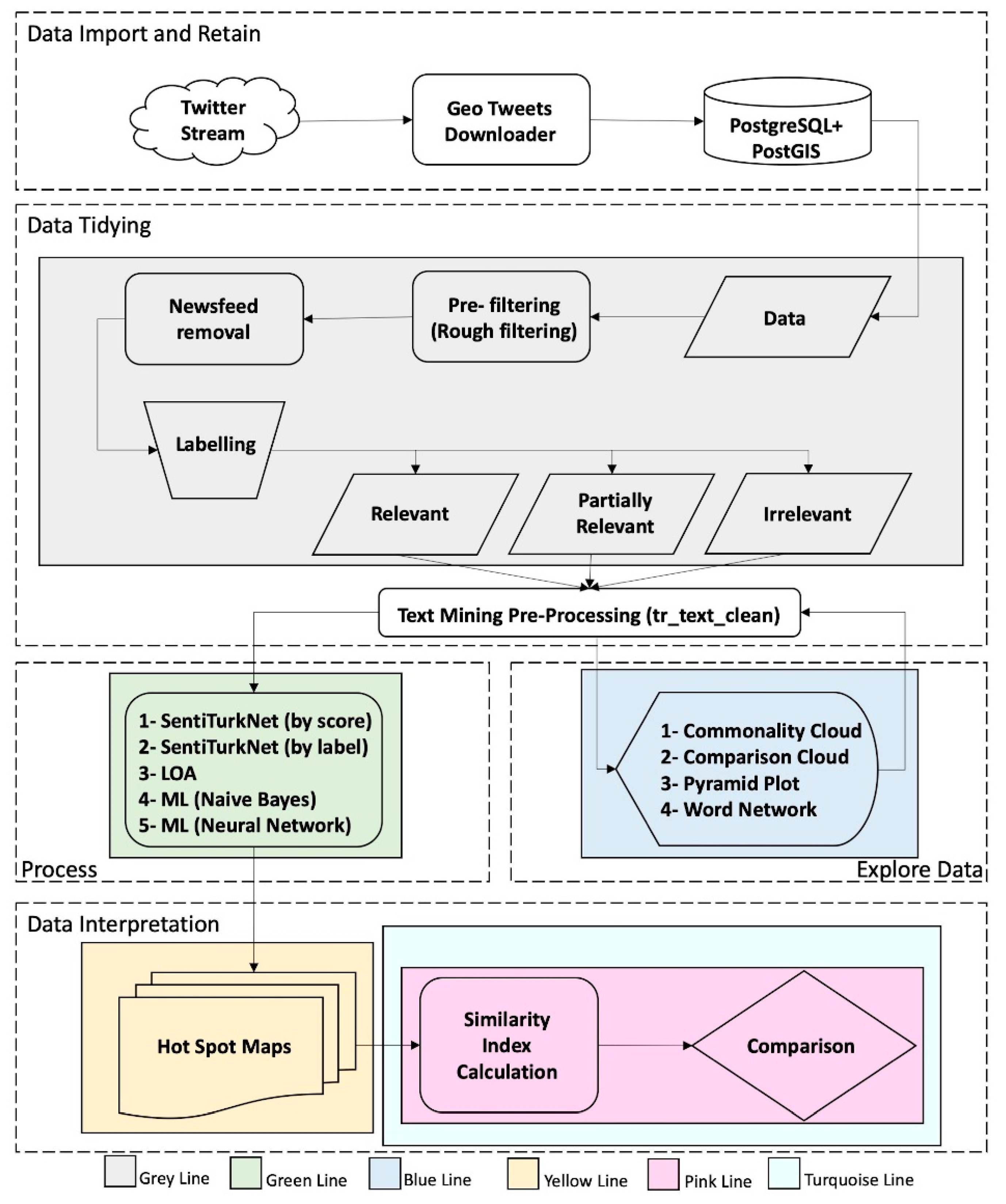
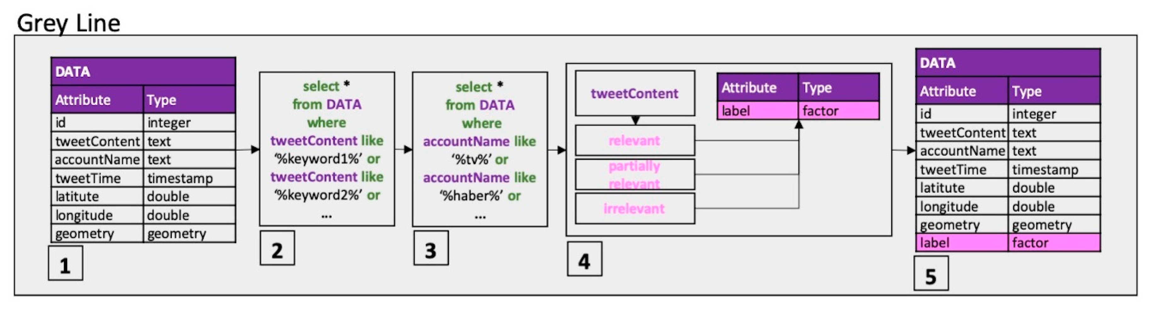
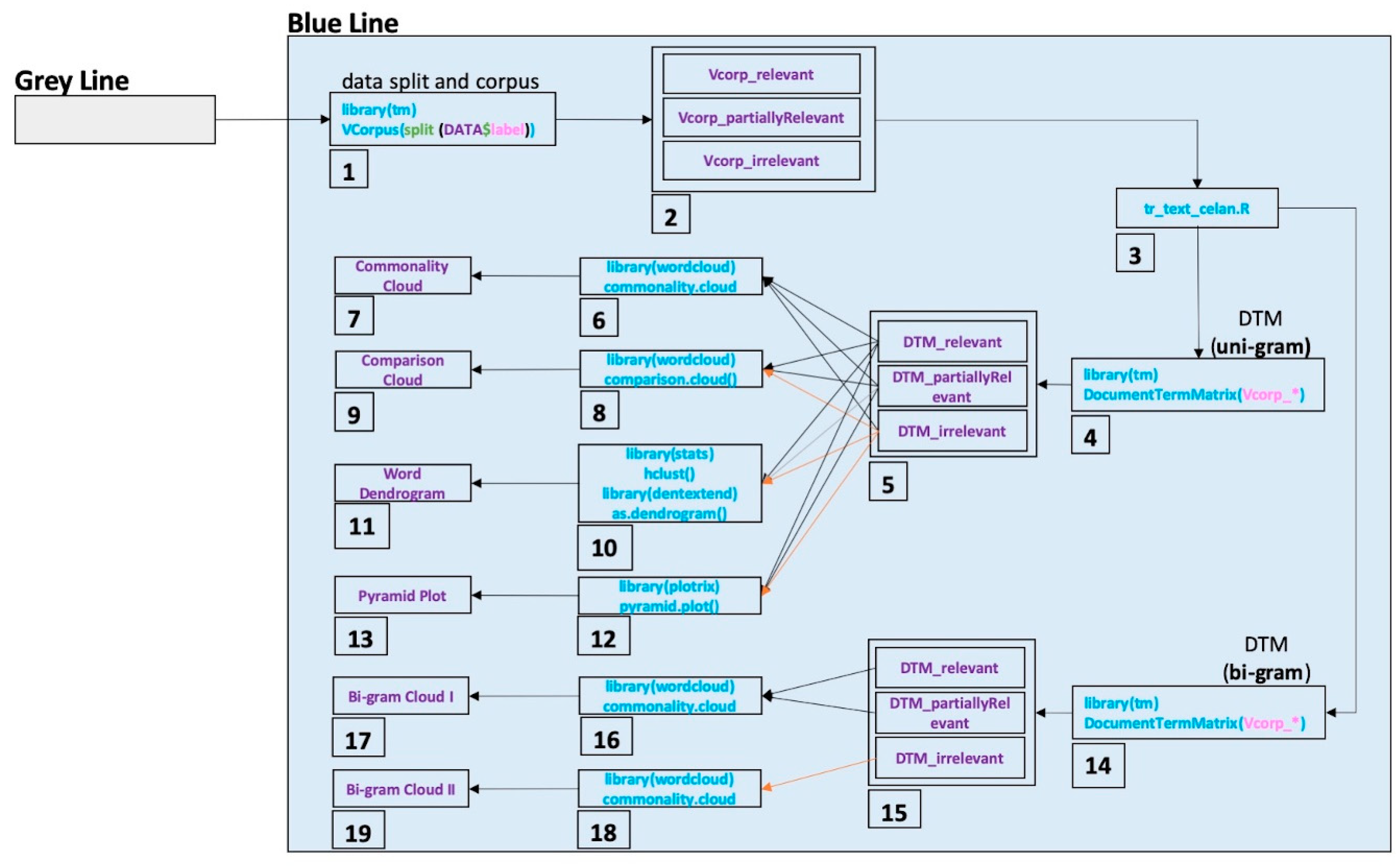
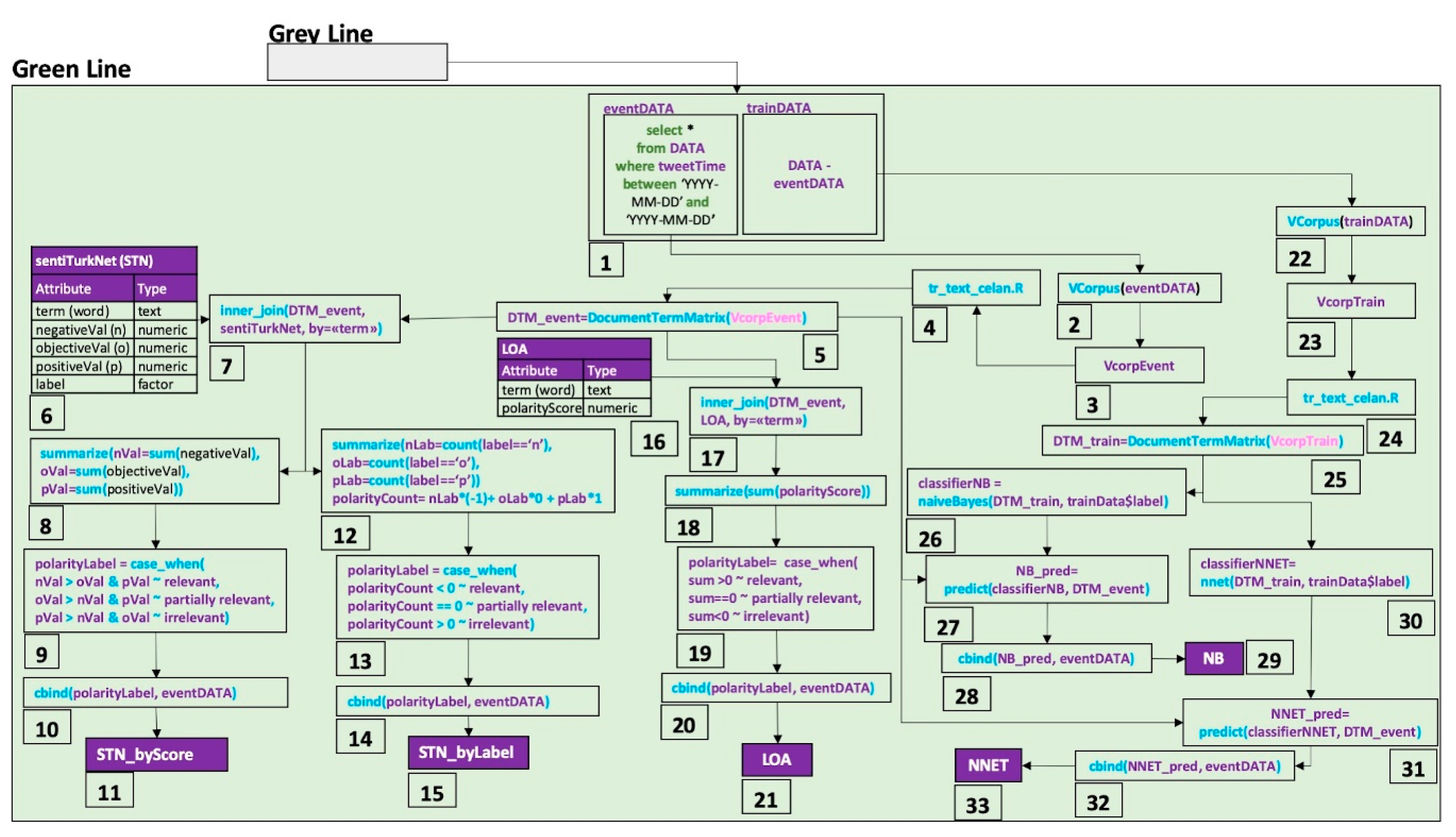
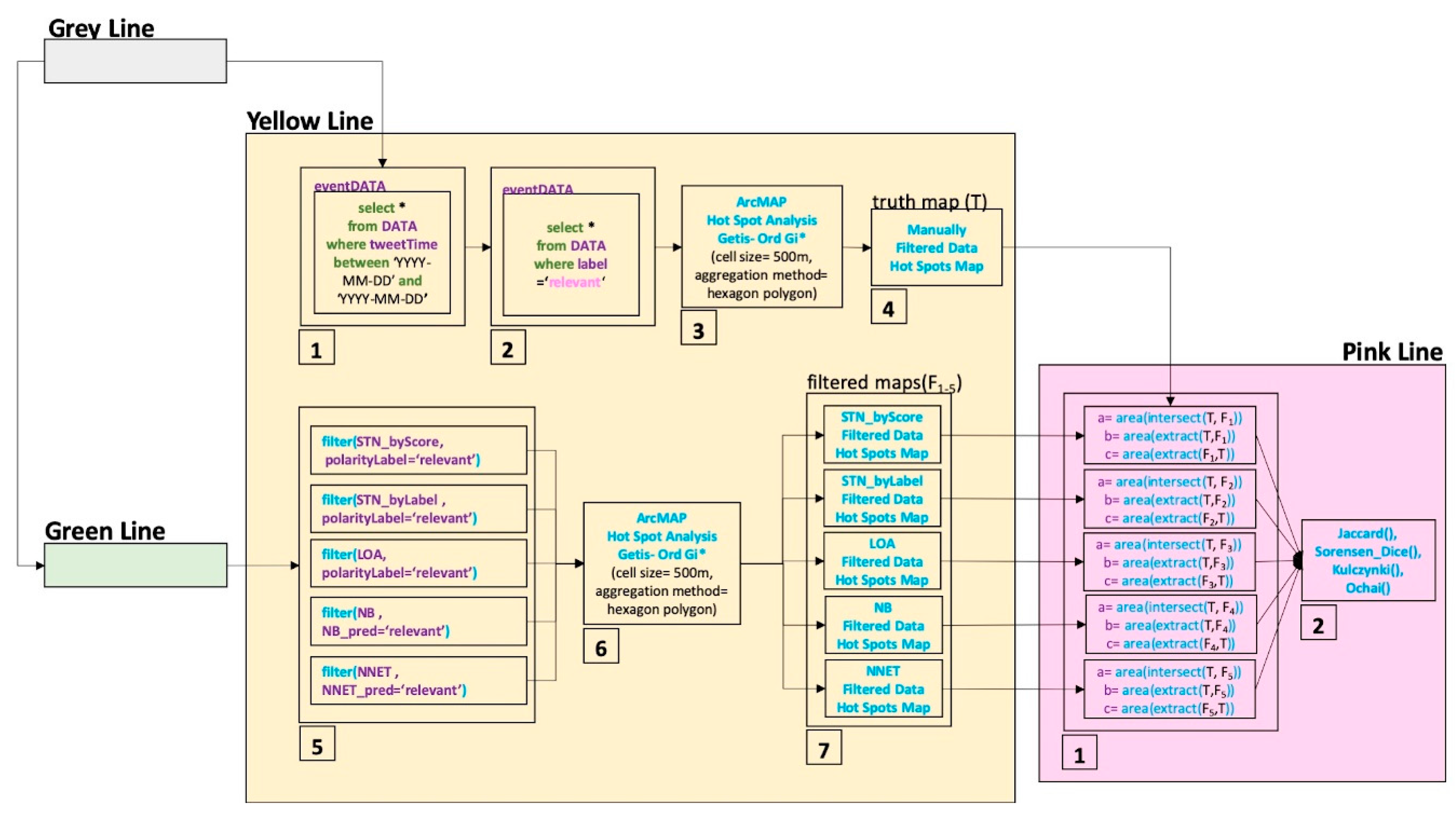
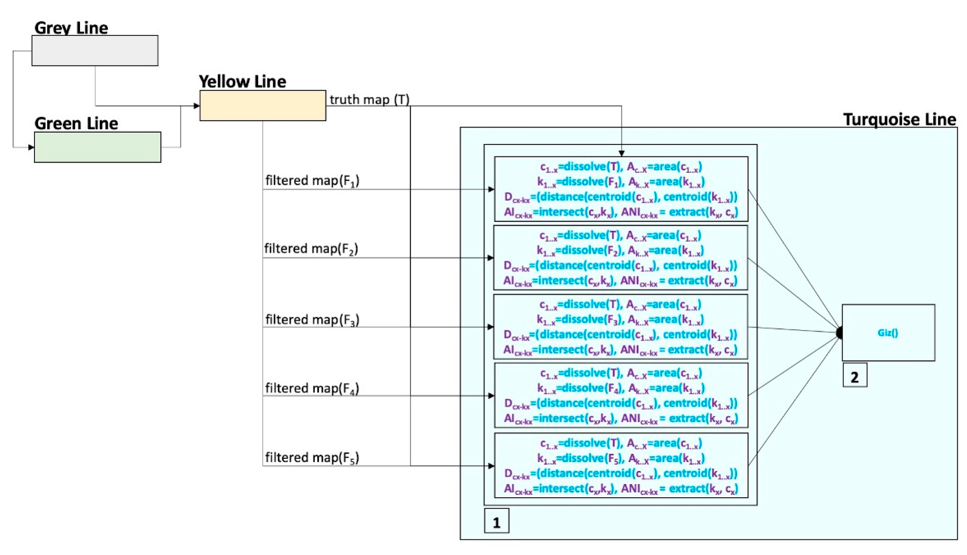
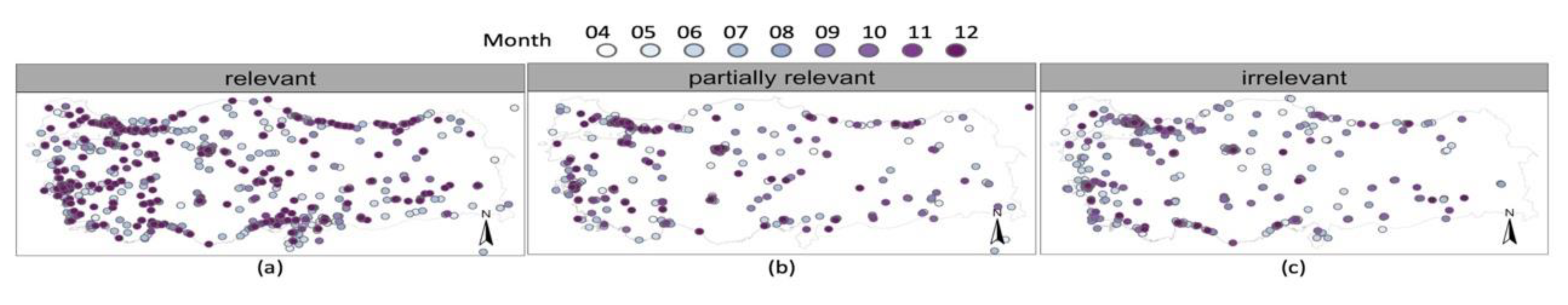
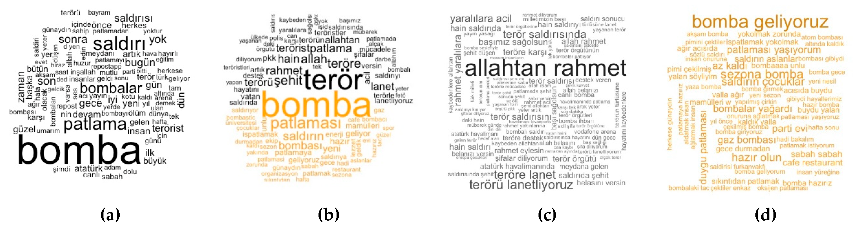
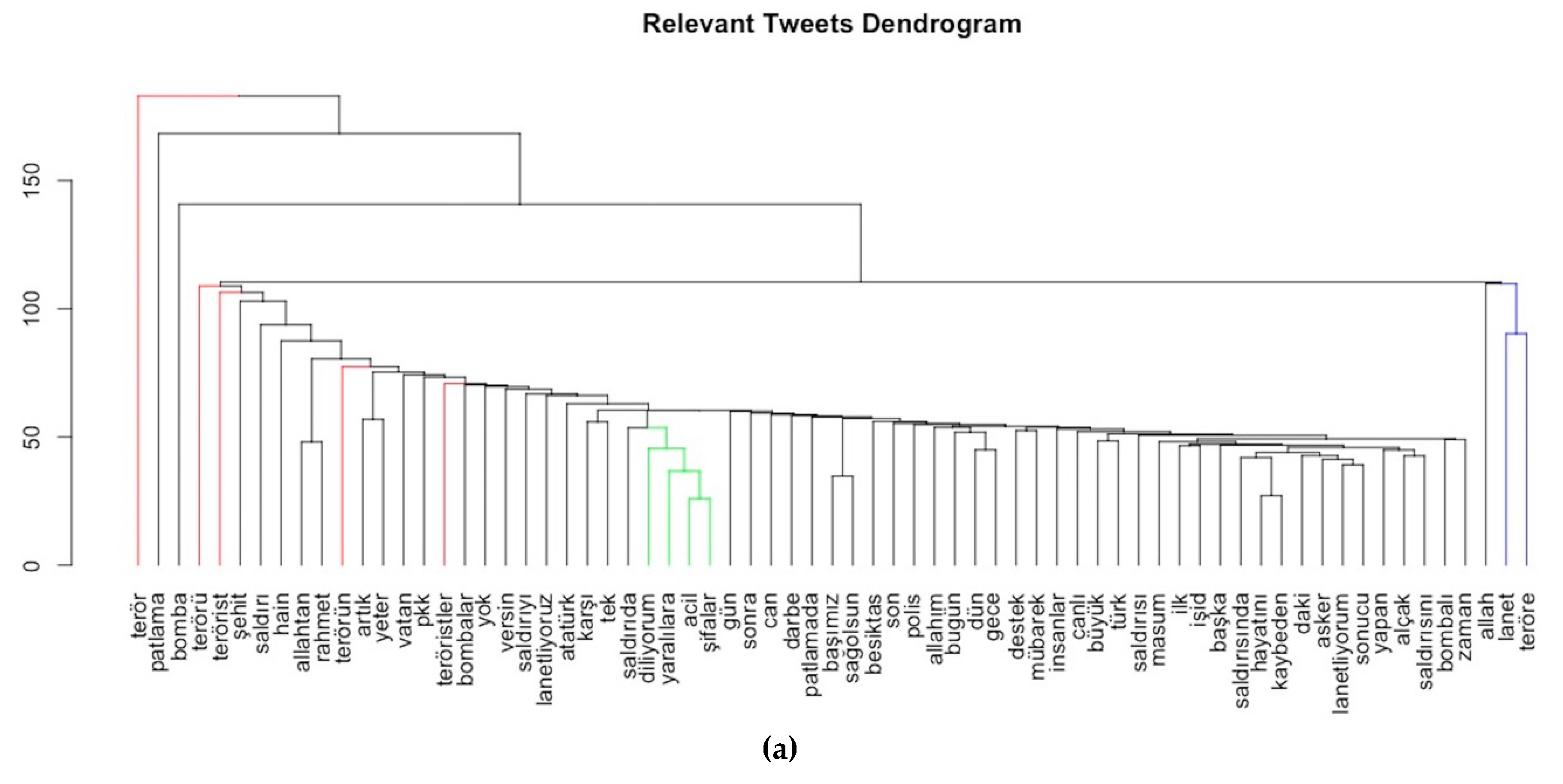
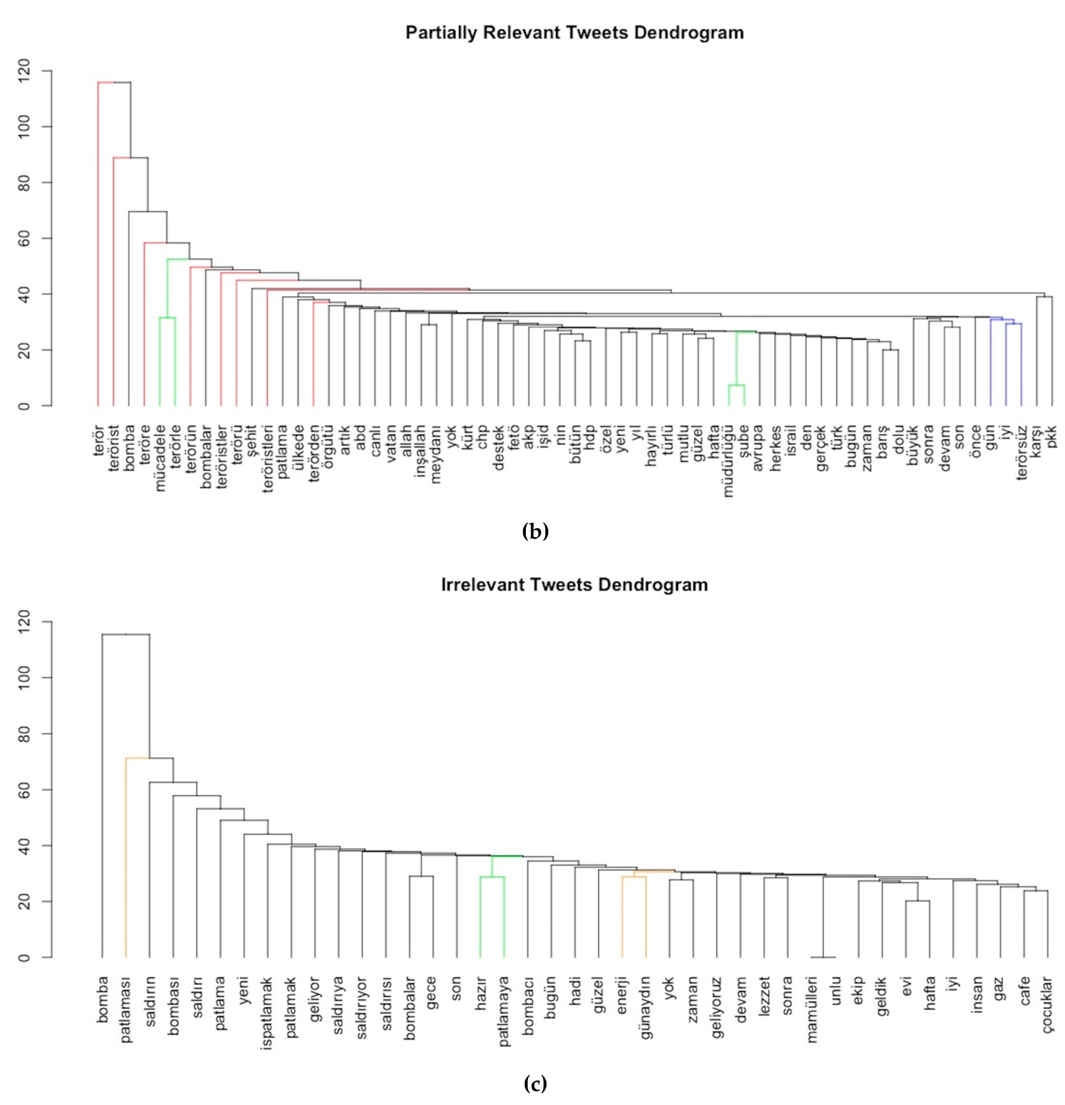
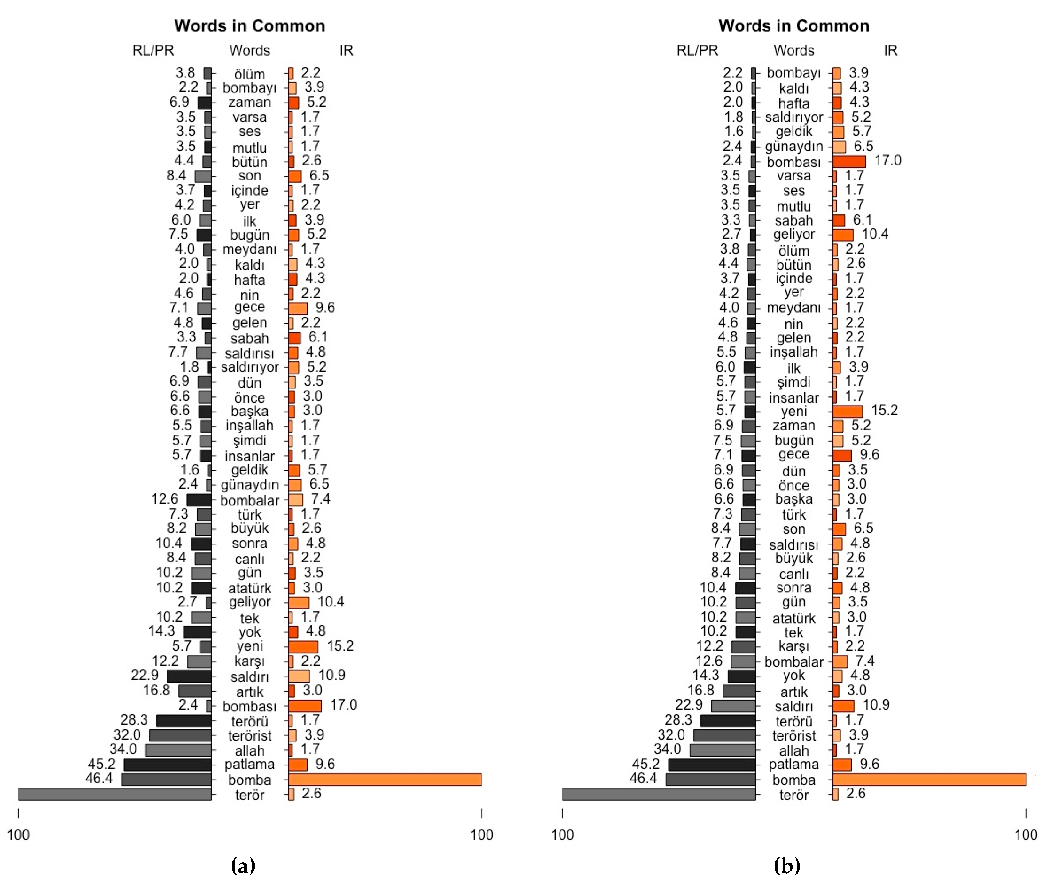
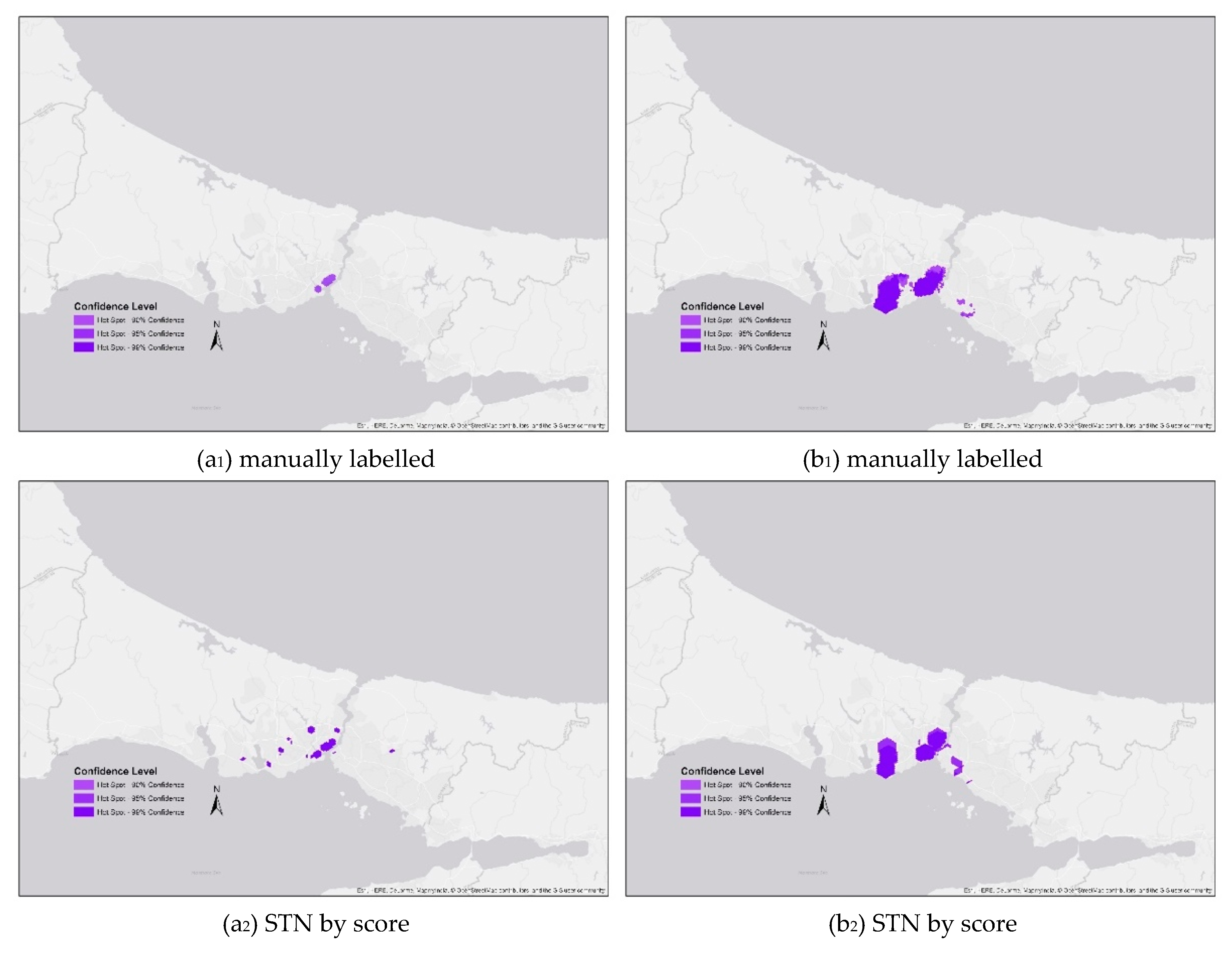
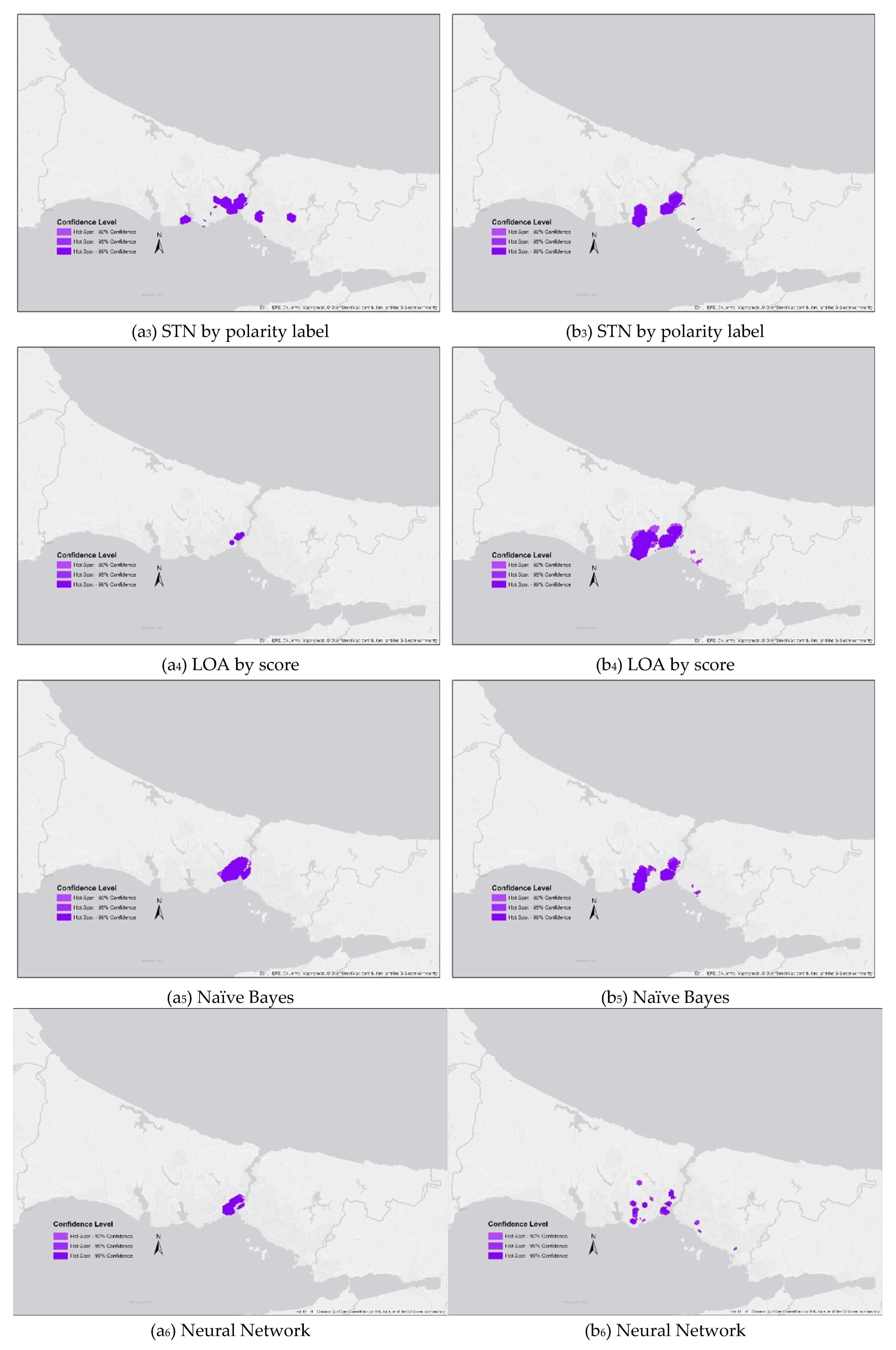