Watershed Segmentation Algorithm Based on Luv Color Space Region Merging for Extracting Slope Hazard Boundaries

Abstract

To accurately identify slope hazards based on high-resolution remote sensing imagery, an improved watershed segmentation algorithm is proposed. The color difference of the Luv color space was used as the regional similarity measure for region merging. Furthermore, the area relative error for evaluating the image segmentation accuracy was improved and supplemented with the pixel quantity error to evaluate the segmentation accuracy. An unstable slope was identified to validate the algorithm on Chinese Gaofen-2 (GF-2) remote sensing imagery by a multiscale segmentation extraction experiment. The results show the following: (1) the optimal segmentation and merging scale parameters were, respectively, minimum threshold constant C for minimum area A_min of 500 and optimal threshold D for a color difference of 400. (2) The total processing time for segmentation and merging of unstable slopes was 39.702 s, much lower than the maximum likelihood classification method and a little more than the object-oriented classification method. The relative error of the slope hazard area was 4.92% and the pixel quantity error was 1.60%, which were superior to the two classification methods. (3) The evaluation criteria of segmentation accuracy were consistent with the results of visual interpretation and the confusion matrix, indicating that the criteria established in this study are reliable. By comparing the time efficiency, visual effect and classification accuracies, the proposed method has a good comprehensive extraction effect. It can provide a technical reference for promoting the rapid extraction of slope hazards based on remote sensing imagery. Meanwhile, it also provides a theoretical and practical experience reference for improving the watershed segmentation algorithm.

1. Introduction

Slope hazards (referring to unstable slopes, landslides, and collapses) are common geological phenomena that have strong effects on the environment around the hazard body and on the safety of human lives and property [1]. Development of remote sensing technology provides a more efficient means for extracting slope hazards. To date, many slope hazard extraction studies have been performed based on image classification and segmentation methods. Nevertheless, most of the previous extraction methods are still rely on visual interpretation of the images based on the Geographic Information System (GIS) software. It not only requires the technicians to be highly experienced in geosciences and interpretation, but also necessitates a large investment of manpower and time, leading to low production efficiency and making the extracted information subjective and imprecise. This makes it difficult to meet the requirements to apply slope hazard extraction to post-hazard emergency investigation and hazard assessment [2]. With the rapid development of high-resolution remote sensing image segmentation technology, automatic extraction of slope hazard boundaries is becoming increasingly feasible [3,4,5,6]. Among the available image segmentation techniques, the watershed segmentation algorithm is proposed based on the color differences of image pixels. A better segmentation effect can be obtained for those images with more obvious contrast [7]. Slope areas have highly consistent textures and spectrums on a high-resolution remote sensing image, but the hues are usually different from that of the surrounding background. This provides the basis for automatic extraction of slope hazard boundaries using watershed image segmentation technology.

Increasing research efforts have been recently devoted to developing the watershed segmentation algorithms. For example, the overflow method [8,9] was proposed and applied. Furthermore, the segmentation method was used from grey images to color images [10]. The processing speed was also improved by the precipitation watershed segmentation [11]. The connected component operator was used to improve the watershed segmentation algorithm [12]. Soille systematically summarized the literature on the watershed segmentation algorithm [13]. To date, the algorithm has been widely used in the field of remote sensing image information extraction [14,15,16]. In addition, dozens of improved watershed segmentation algorithms have been also proposed to solve the problems of image over-segmentation and obvious algorithm noise, such as an algorithm based on efficient computation of the shortest paths [17], a texture marker-controlled watershed segmentation algorithm [18], an edge embedded marker-based watershed segmentation algorithm [19], a wavelet transform in combination with marker-based watershed segmentation algorithm [20], and image segmentation including image enhancement and noise removal techniques with Prewitt’s edge detection operator [21]. The improved methods include pre-improvement, post-improvement, or both; among these, the region merging based watershed segmentation algorithm [16,22,23] can be used after segmentation based on the characteristics of the region texture, color, and shape information. Chen adopted fuzzy clustering with spatial patterns for post-improvement [24]. Additionally, some scholars used prior knowledge for pre-improvement and regional combination for post-improvement [25,26]. Studies on image brightness equalization based on color space measurement in the lab color space [27] have been performed gradually to obtain better segmentation results by developing watershed image segmentation and region merging methods. Meanwhile, the red–green–blue (RGB) color model has been used in traditional image processing. In such a color model, three components of an image are highly correlated. When the brightness is changed, all the three components will be changed. This property of the RGB color definition makes the model unsuitable for the image segmentation. Therefore, watershed segmentation algorithms based on the intensity–hue–saturation (IHS) color model [28] and improved color space [29] were developed, which have been jointly used with clustering algorithms for image classification.

The accuracy of subsequent information analysis and processing has been found to be directly affected by the image segmentation quality [30,31]. Therefore, it is necessary to comprehensively and objectively evaluate the image segmentation methods [32]. Evaluation of segmentation accuracy is considered to be equally important as the image segmentation technology [33]. Various qualitative and quantitative methods have been proposed [34,35,36,37]. However, there are many uncertainties for remote sensing image segmentation. It is recognized as an issue for quantitatively evaluating the image segmentation [33,38,39]. To assess the segmentation quality, various indicators were proposed [40,41,42,43,44,45,46,47]. Although these methods have supported the evaluation of the segmentation effect, the subjective evaluation method is still the most commonly used method [33].

It is highly necessary to improve the accuracy and simplify the evaluation criteria for extracting slope hazard boundary based on remotely sensed images. A Chinese Gaofen-2 (GF-2) image was processed in the Luv color space. The post-processing-based region merging method was used to improve traditional simulated immersion watershed algorithm. At the same time, an improved evaluation criterion for watershed segmentation was also proposed. Finally, a complete Luv-color space-based region merging watershed segmentation (hereafter refers to as Luv-RMWS) was developed to extract slope hazard boundary. The primary sections are arranged as follows: (1) study area and preprocessing are shown in Section 2; (2) the technical flowchart and algorithm descriptions of Luv-RMWS are presented in Section 3; (3) proposed accuracy evaluation criteria including area relative error and pixel quantity error are shown in Section 4.3; (4) comparison of segmentation results and evaluation of extraction accuracy and processing time are shown in Section 5; and (5) corresponding discussions concerning optimal scale parameters and extraction effect are given in Section 6.

2. Study Area and Data Preprocessing

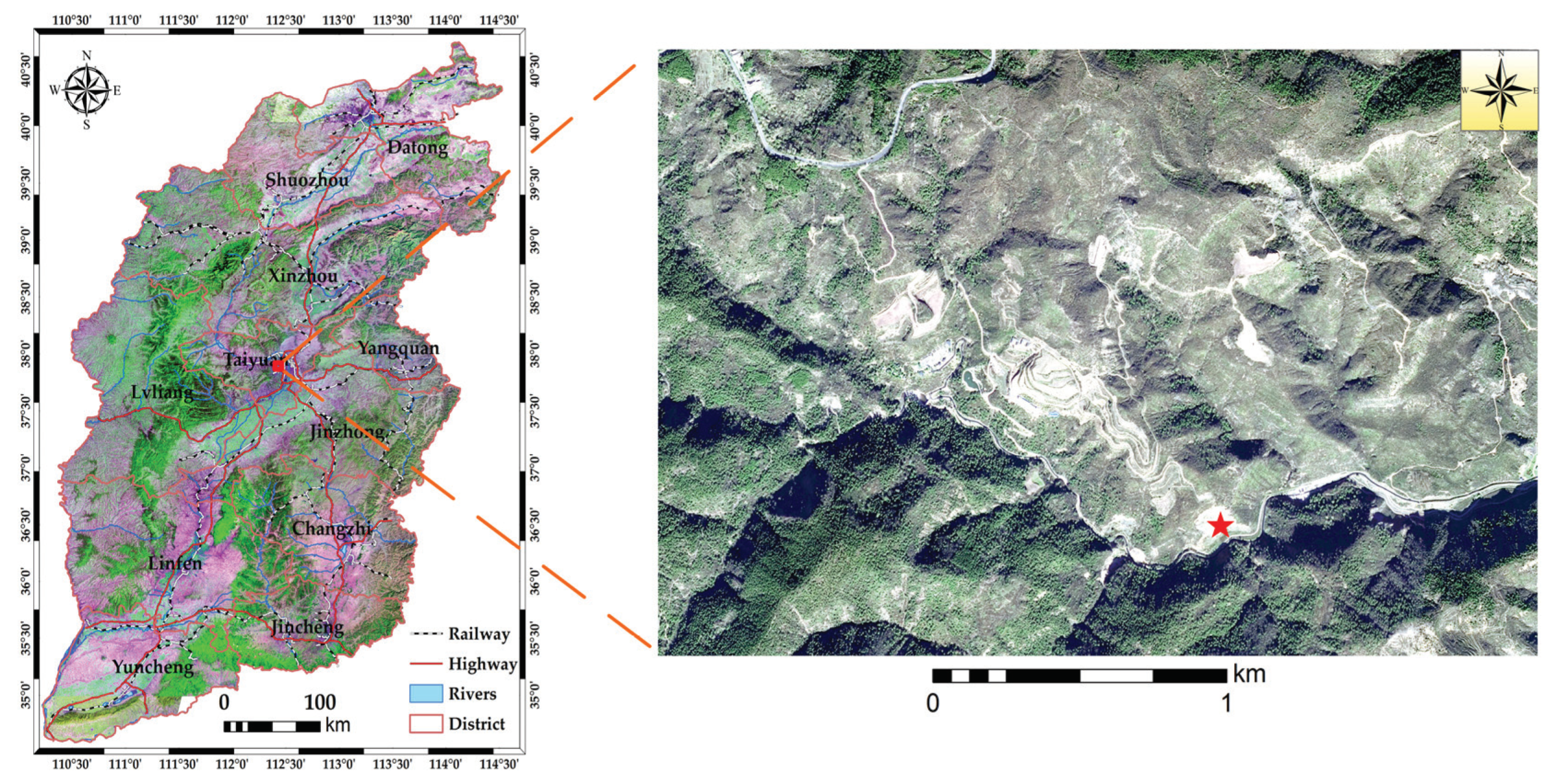
2.1. Study Area

The study area is located in Taohuagou, Du’erping Mining Area, Xishan Coalfield, Taiyuan City, Shanxi Province, China (Figure 1). The area is characterized by unstable slopes, landslides, collapses, and other geological hazards. In this paper, an unstable slope (marked by ★ in Figure 1) was selected to extract its boundary based on the proposed Luv-RMWS method.

2.2. Data Sources and Preprocessing

A GF-2 remote sensing image of 2015 with a spatial resolution of 1 m was selected as the experimental data (Figure 2a). Geometric and orthographic corrections were carried out based on the 1:10,000 topographic map produced by aerial photogrammetry in 1999. Additionally, image fusion, clipping, and contrast enhancement were adopted to highlight the slope information (Figure 2b).

3. Methodology

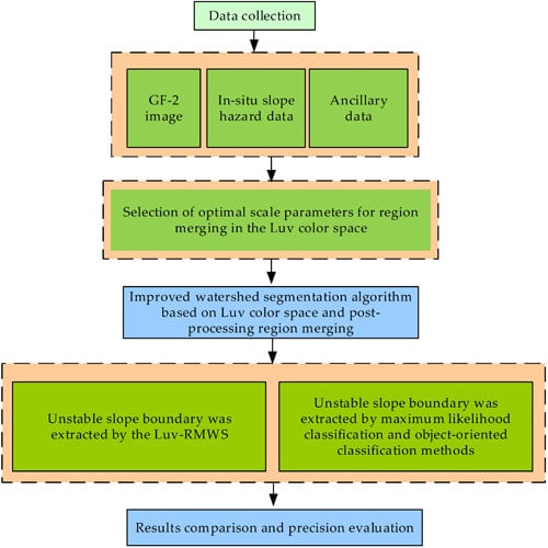
3.1. Technical Procedure

Watershed segmentation algorithm can be implemented by many methods. One of the most commonly used is the simulated immersion algorithm, first proposed by Vincent and Soille [8]. In this study, it is performed using the simulated immersion algorithm (Figure 3).

3.2. Luv Color Space and Transformation

CIE1976 Luv is a color space derived directly from the CIE XYZ space that is used to linearize chromatic aberration perception. Here, L ranging from 0 to 100 is the brightness of a pixel that is consistent with the L in Lab color space, while u and v are the chromaticity coordinates and range from –100 to 100 [48]. CIE1976 specifies the conversion between RGB and XYZ, and XYZ and Luv. The conversion procedure is as follows:

1. The color value of each channel of the image is denoted as R, G, B, respectively.

2. Assuming it is the standard RGB color space coordinate, the relatively uniform chromaticity coordinate L, u, v can be obtained through the color space conversion [49].

$$\left[\begin{array}{l}\mathrm{X}\\ \mathrm{Y}\\ \mathrm{Z}\end{array}\right]=\left[\begin{array}{ccc}0.430& 0.342& 0.178\\ 0.222& 0.707& 0.071\\ 0.020& 0.130& 0.939\end{array}\right]\left[\begin{array}{l}\mathrm{R}\\ \mathrm{G}\\ \mathrm{B}\end{array}\right]$$

(1)

$$\mathrm{L}=\{\begin{array}{c}166\ast {(\mathrm{Y}/{\mathrm{Y}}_{\mathrm{n}})}^{1/3}-16\\ 903.3\ast (\mathrm{Y}/{\mathrm{Y}}_{\mathrm{n}})\end{array}\begin{array}{c}\mathrm{I}\mathrm{f}(\mathrm{Y}/{\mathrm{Y}}_{\mathrm{n}})>0.008856\\ \mathrm{I}\mathrm{f}(\mathrm{Y}/{\mathrm{Y}}_{\mathrm{n}})\le 0.008856\end{array}$$

(2)

$$\{\begin{array}{c}u=13L(u^{\prime }-{u_n}^{\prime })\\ v=13L(v^{\prime }-{v_n}^{\prime })\end{array}$$

(3)

where ${u_n}^{\prime }$ and ${v_n}^{\prime }$ are the coordinates of CIE standard light source and are the tristimulus values given by

$$u^{\prime }=4X/(X+15Y+3Z)$$

(4)

$$v^{\prime }=9Y/(X+15Y+3Z)$$

(5)

$${u_n}^{\prime }=4X_n/(X_n+15Y_n+3Z_n)$$

(6)

$${v_n}^{\prime }=9Y_n/(X_n+15Y_n+3Z_n)$$

(7)

In the case of 2° observer and C light sources, ${u_n}^{\prime }=0.2009$, ${v_n}^{\prime }=0.4610$.

In the Luv color space, the difference between any two colors is referred to as chromatic aberration. Chromatic aberration is the distance between color positions expressed as ∆E, i.e., the chromatic aberration between two colors is calculated as:

$$\Delta E={(\Delta L^2+\Delta u^2+\Delta v^2)}^{1/2}$$

(8)

where ∆L is the difference in brightness, and ∆u and ∆v are the differences between two colors in the u and v directions, respectively.

3.3. Region Merging Similarity Measure Based on Luv Color Space

To evaluate the color quality of remote sensing images, Xue evaluated the brightness equalization after transforming the RGB color space into the Lab color space. This approach is to divide the image to m × n small areas and calculate the mean of the gray value or L for each small area image, and then take the mean value as the brightness value to form a new image by a resampling procedure. Then, the quadric surface is fitted according to the region block, and the mean square deviation σ² (0, 255) is calculated, which is the image brightness equalization index [27,50]. It is clear that this approach is related to region merging. The brightness equalization approach seeks to find the brightness difference between image blocks and then evaluate the overall brightness deviation of the image, while the region merging approach aims to find the difference between segmented regions and then determines whether to merge the regions according to the similarity measure. The method used in this study is based on a combination of these research findings and differs from the traditional region merging approach. The watershed segmentation algorithm usually uses the RGB and IHS color spaces. The Luv color space, similar to the Lab color space, is selected as the regional similarity calculation basis of the algorithm, and the algorithm was improved based on the homogeneity maximization criterion [51].

3.3.1. Optimal Segmentation Scale Parameters

The key parameter for selecting the scale parameters by the watershed segmentation algorithm is the threshold value (A_min) of the minimal region. Defining M as the row value of an image, N as the column value, and C as a given constant, and taking the number of pixels as the minimum area to determine the threshold, we obtain:

$$A_{\min }=(M\times N)/C$$

(9)

It is clear that A_min is not a fixed value and will have different values for different sizes. Generally, the optimal A_min can be determined by a trial-and-error test, but it is crucial to properly determine the value of constant C.

3.3.2. Optimal Merging Scale Parameters

Chromatic aberration is the Euclidean distance between positions of the colors in the Luv color space. The color similarity of two positions can be determined using the color difference threshold, by integrating the homogeneity maximization criterion and light intensity threshold similarity measures. In this paper, the chromatic aberration of Luv color space is used to determine the similarity value of regions in the segmentation unit. If the chromatic aberration is within the threshold range, the regions are similar and will be merged; otherwise, the regions will not be merged. This is carried out to achieve merging of the segmentation results of the image.

Suppose that R_i and R_j are the two regions of G image divided by the watershed segmentation. To eliminate the impact of the size difference of regions during merging process, an improved calculation equation (Equation 10) was proposed to obtain the chromatic aberration of adjacent regions in the Luv color space.

$$d_i=\frac{\left|R_i\right|·\left|R_j\right|}{\left|R_i\right|+\left|R_j\right|}\sqrt{{\displaystyle \sum _{c=L,u,v}{(F_c(R_i)-F_c(R_j))}^2}}\hspace{1em}i=1,2,3\dots ,n;\hspace{1em}j=1,2,3\dots ,n$$

(10)

where |R_i|, |R_j| are the numbers of pixels contained in image areas R_i and R_j, respectively; F_c(R_i), F_c(R_j) are the average colors of image areas R_i and R_j, and n is the number of adjacent areas.

The color difference is used to determine the similarity between the current minimum region and its adjacent regions. If d_i ≤ 1, the colors of two regions cannot be distinguished, so a smaller d_i indicates greater similarity between the colors [52]. In region merging, it is necessary to determine whether the colors of adjacent regions are similar. Therefore, threshold size d_i is determined by theoretical analysis and empirical verification. Let the color difference threshold be D; if the color difference threshold is set, region merging of the segmentation results is completed under the constraint $\sqrt{D}$ until similar region merging can no longer be performed.

The region merging algorithm based on the homogeneity maximization criterion of Luv color space is given by:

1. The pixels of in image are converted from RGB values to Luv values after watershed segmentation, and the average Luv value in each region is calculated as the Luv value of this region. The segmentation result is converted from RGB to Luv color space, which can be used for calculating the similarity of region merging.

2. Four neighborhood arrays of each region with Luv mean value are set as the color of the region.

3. Threshold A_min for determining the minimal area is calculated according to the C and image size. All areas are scanned in turn, and the minimal area is found as the initial combined area. If the number of pixels of an area is less than the number of image pixels divided by C, it will be considered as a minimal area for calibration; otherwise it is not.

4. To determine the minimal area, all adjacent areas are traversed to obtain the average Luv value of adjacent areas. The value of chromatic aberration d_i is calculated between the minimal area and adjacent areas, and regions with the closest similar regions are found to be merged based on the judgment method of threshold D of chromatic aberration. When $d_i\le \sqrt{D}$, the regions are merged; otherwise, when $d_i>\sqrt{D}$, the regions do not merge. The calculation equation of chromatic aberration is shown in Equation (10).

5. The information of adjacent regions is refreshed to form a new region, after the minimal region is merged with similar regions close to it. The Luv value of the new region is the mean value of the Luv value of the two regions before merging.

6. The new area is judged after merging; return to step 4 if it is still a minimal region; otherwise, proceed to the next step.

7. All the areas are judged. If all regions have merged, it ends; otherwise return to step 3.

8. The Luv values of all merged areas are converted into RGB values for better display effect, so the final result of segmentation area in the image is displayed in RGB values.

4. Comparative Methods and Accuracy Evaluation

4.1. Maximum Likelihood Classification

Maximum likelihood classification (MLC) is also known as Bayes classification. To calculate the probability (likelihood) for each pixel in each category, the pixels are categorized using the maximum likelihood [53]. It is assumed that there are k types of ground objects in the remote sensing image, and category i of a ground object is represented by w_i, and the prior probability for each category is P(w_i). Given an unknown category X, the conditional probability appearing in class w_i is P(X|w_i) (also called the likelihood probability of w_i). According to Bayes′ theorem, the posterior probability of category can be obtained as follows:

$$P(w_i|X)=\frac{P(X|w_i)P(w_i)}{P(X)}=\frac{P(X|w_i)P(w_i)}{{\displaystyle \sum _{i=1}^{k}P(X|w_i)}P(w_i)}$$

(11)

where P(X) is a constant for each category, and the discriminant function can be simplified as follows:

$$P(w_i|X)=P(X|w_i)P(w_i)$$

(12)

In the Bayes classifier, the posterior probability of category X is used as the discriminant function to determine the specific category. When P(w_i|X) > P(w_j|X) is satisfied for j = 1, 2, …, k, j ≠ i, then X belongs to class w_i.

4.2. Object-Oriented Classification

A multiscale segmentation algorithm is adopted in object-oriented classification (OOC), the key of which is determining the optimal segmentation parameters. At present, repetitive experiments are often carried out on images before segmentation, and the best segmentation parameters are visually judged a trial-and-error test. The overall heterogeneity of image segmentation objects is controlled by spectral and shape heterogeneity parameters [54], and the expression is given by

$$h={\omega }_{color}\times h_{color}+{\omega }_{shape}\times h_{shape}$$

(13)

where h is the overall heterogeneity of the object; h_color is spectral heterogeneity; h_shape is shape heterogeneity; ω_color is the weight of spectral heterogeneity; ω_shape is the weight of shape heterogeneity, and ω_color + ω_shape = 1. Shape heterogeneity is comprehensively expressed by smoothness and compactness, and the equation is given by

$$h_{shape}={\omega }_{com}\times h_{com}+{\omega }_{smooth}\times h_{smooth}$$

(14)

where ω_com is the custom compactness weight, ω_smooth is the custom smoothness weight, and the sum of ω_com and ω_smooth is 1.

4.3. Accuracy Evaluation Criteria

As mentioned above, the existing evaluation methods mainly focus on visual evaluation, or are based on the applicable conditions to evaluate the accuracy of the algorithm. How to be simple and effective, and quantitatively evaluate the segmentation accuracy of the watershed algorithm is still a difficult issue [33,38,39]. Based on the analysis of the existing research results, the area relative error criterion was proposed in this paper, supplemented by the pixel quantity error criterion for a comprehensive evaluation of watershed image segmentation accuracy.

(1) Area relative error criterion (accuracy factor: δ_A)

Usually, the reference feature value in the reference data is represented by R_f, while the actual feature value in the segmented image result is represented by S_f, and then their absolute difference is given by [55].

$$AUMA=|R_f-S_f|$$

(15)

Here, AUMA is the accuracy factor used for evaluation of the image segmentation results, and the characteristic quantity is usually represented by the area. A smaller AUMA corresponds to higher segmentation accuracy, and otherwise the accuracy is lower.

However, it is not reasonable to use the absolute value of the difference between the target segmentation and the reference area to represent image segmentation accuracy in the error theory, because the size of the error relative to the reference area is unknown. Theoretically, the area of the image segmentation target is the same as the reference area for the optimal segmentation algorithm. However, regardless of the quality of the algorithm, the segmentation area will always differ from the reference area, and an error will be present. Similarly, it is unknown whether the evaluation area is changed by the orthomorphic projection. Therefore, the image segmentation effect can be better represented by the ratio of segmentation area to reference area. Similarities between two quantities can be effectively evaluated simply by using the ratio between them, but to evaluate accuracy, we should use relative error according to the theory of measurement error.

An inspection of Equation (15) shows that AUMA is an absolute error that represents the absolute value by which the segmentation result area deviates from the reference value. The percentage calculated by AUMA and the reference value can represent the percentage of absolute error relative to the true value, and can better reflect the validity and reliability of the segmentation precision. Therefore, the area relative error was proposed as a criterion for evaluation of the image segmentation accuracy in this paper, and is calculated as follows.

Let A₀ be the target area value in the benchmark data, and A_S be the target area value in the segmentation image result, then their relative error δ_A is given by

$${\delta }_A=\frac{|A_s-A_0|}{A_0}\times 100\%$$

(16)

where δ_A is the area accuracy factor used for evaluation of the image segmentation result. A smaller δ_A corresponds to higher segmentation accuracy, and otherwise the accuracy is lower.

(2) Pixel quantity error criterion (accuracy factor: δ_P)

Image segmentation accuracy is represented by the number of pixels with incorrect segmentation obtained from the overlay of the reference image and the segmentation result divided by the total number of pixels. This criterion is consistent with the area relative error and was used to evaluate accuracy from a different perspective. In this paper, the pixel number error was also selected as an evaluation criterion for image segmentation accuracy. The pixel number error is obtained as follows.

Let P_t and P_w represent the numbers of pixels that are correctly and incorrectly segmented, respectively, then the error rate δ_P is given by

$${\delta }_P=\frac{P_w}{P_t+P_w}\times 100\%$$

(17)

where δ_P provides an overall evaluation of the image segmentation accuracy. A smaller δ_P corresponds to higher segmentation accuracy, and otherwise the accuracy is lower.

The criteria for evaluation of the image segmentation accuracy of the watershed algorithm are shown in

Table 1. Criteria for evaluating segmentation accuracy of watershed algorithm.

Indicator	Equation	Note
δA	${\delta }_A=\frac{|A_s-A_0|}{A_0}\times 100\%$	Smaller δA indicates higher segmentation accuracy, and otherwise the accuracy is lower.
δP	${\delta }_P=\frac{P_w}{P_t+P_w}\times 100\%$	Smaller δP indicates higher segmentation accuracy, and otherwise the accuracy is lower.

. At present, the indicators derived from confusion matrix are commonly used to evaluate image-based classification. They include overall accuracy ($P_C$), user′s accuracy ($P_{u_i}$), producer′s accuracy ($P_{A_j}$), and the Kappa coefficient ($K_{hat}$) [56,57]. In order to evaluate the reliability of the image segmentation accuracy evaluation criteria proposed in this paper, $P_C$, $P_{u_i}$, $P_{A_j}$, and $K_{hat}$ of the extraction results of the three methods are calculated simultaneously for comparison.

5. Results

5.1. Segmentation Results Based on the Experimental Image

To compare the segmentation efficiency and effect, contrast enhancement preprocessing was performed on the test image. The same C and D values were used in the experiments to ensure that the segmentation results were comparable. The segmented images were obtained in Figure 4 were respectively based on the original image (Figure 2a) and contrast-enhanced image (Figure 2b) and the statistical results of the segmentation process are provided in

Table 2. Statistical features derived from the Luv-RMWS algorithm.

Image Category	Patch Number of Watershed Segmentation	Time of Watershed Segmentation (ms)	Number of Patches after Area Merging	Time of Area Merging (ms)	C	D
Original image	103,939	1248	22	74,896	500	400
Enhanced image	62,716	1076	33	38,626	500	400

.

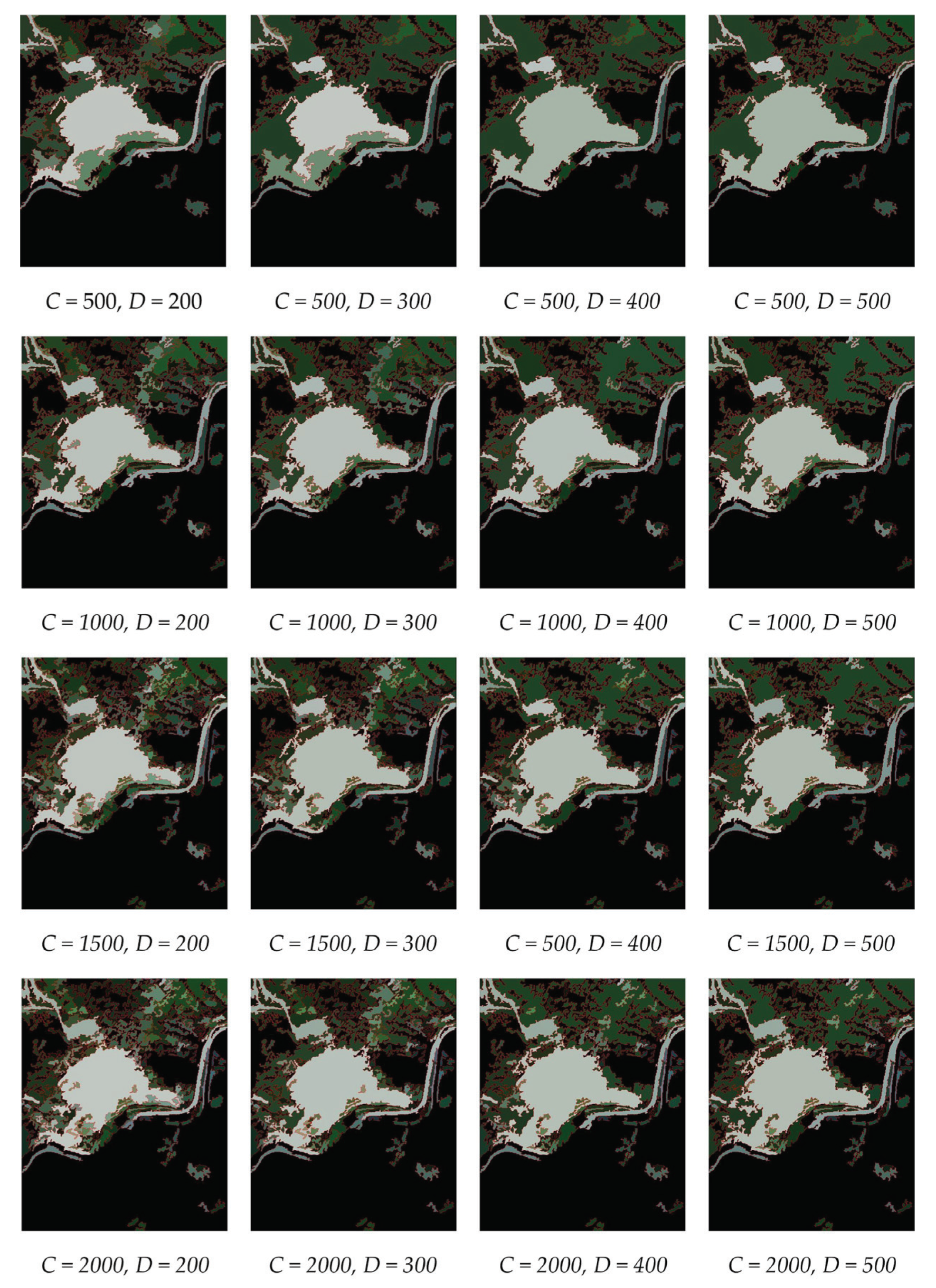
5.2. Selection of Optimal Scale Parameters

To select the optimal segmentation and merging scale parameters, multiscale segmentation experiments were performed on the test images. The C value varied between 100 and 3000 at intervals of 50, and D varied between 100 and 1000 at intervals of 50. The results obtained for different combinations of C values and D values are shown in Figure 5.

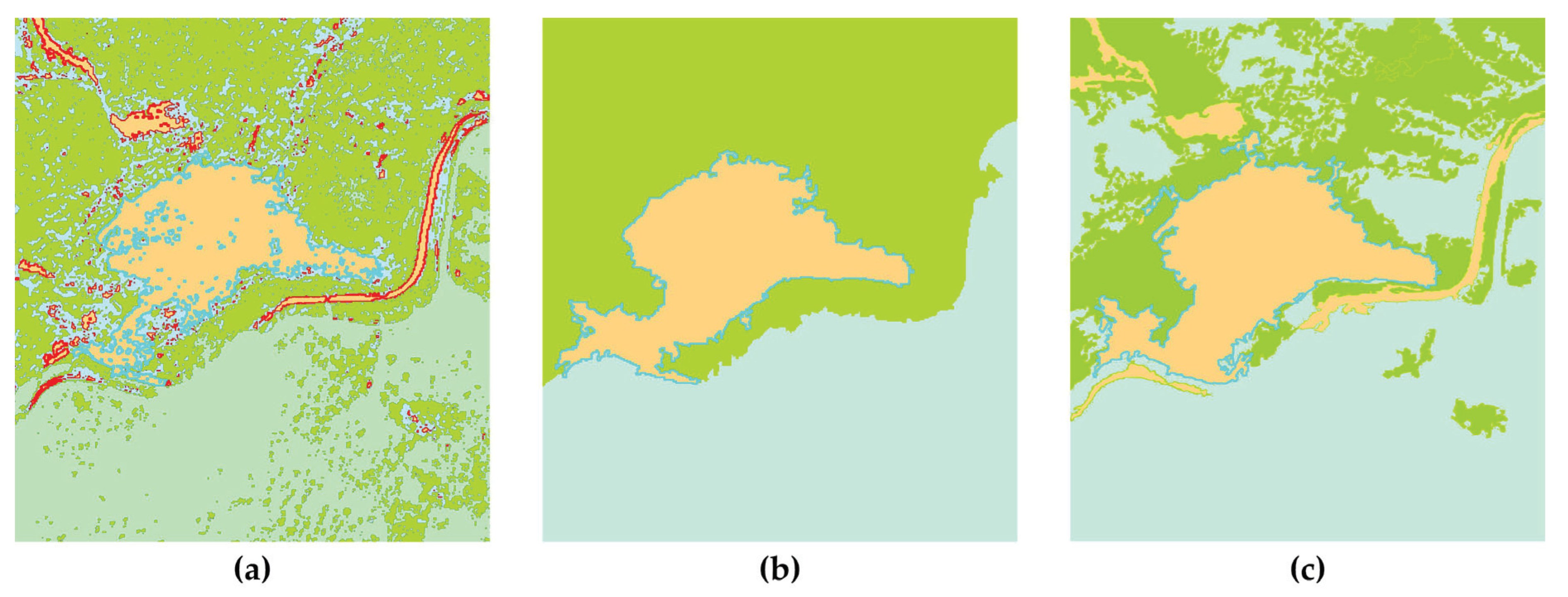
5.3. Extraction of Slope Hazard Boundary

The image classification tool in the spatial analysis toolbox of ArcGIS was used to select the MLC method. The number of classes was set to 4 and a total of 31 sample areas were selected for training. The training results were used as the characteristic data for MLC method, and the results of image supervised classification and vector format were obtained (Figure 6a). By repeating the OOC method experiments using eCognition and visually comparing the results, the optimal segmentation scale parameters were selected as: ω_color = 0.8, ω_shape = 0.2, ω_com = 0.5, and ω_smooth = 0.5, and the vector format of the unstable slope body segmentation extraction results was obtained (Figure 6b). Then, the boundary of the unstable slope body was segmented and extracted by the RSImage-WS platform (Luv-RMWS experimental platform developed based on VC++). The obtained extraction results were shown in vector format in Figure 6c.

To evaluate the accuracy of image segmentation and extraction based on the improved algorithm described in this paper, ArcGIS was used for visual interpretation of the test images. After field verification and correction, the accurate boundary of the target body was obtained as the benchmark data. To obtain the continuous boundary, the "Boundary Clean" function in the ArcGIS spatial analysis toolbox was used to smooth the boundary. Then, the classification data were converted from raster to vector format, and the target map was derived through a comparison of the individual files by overlaying the benchmark data and the experimental image (Figure 7).

5.4. Processing Time

The experimental were carried out using an HP 2211f computer with Intel(R) Core(TM) i3 CPU, main frequency 3.20 GHz, 6.00 GB memory, and a 64-bit operating system. The running time of the MLC method was recorded using an ordinary stopwatch, the OOC method was timed from eCognition software, and the Luv-RMWS method used the program’s built-in timing variable. The obtained experimental times are presented in

Table 3. Comparison of extraction times of unstable slope boundaries in experimental images.

Method	Running Time	Experimental Platform	Note
MLC	381.000 s	ArcGIS	Required more than 1 h for the whole process including sample training and classification, and post-processing such as debris combination.
OOC	11.470s	eCognition	Automatic image segmentation and merging, where segmentation time is 11.470 s, and the number of patches after segmentation was 3.
Luv-RMWS	39.702 s	RSImage-WS	Automatic image segmentation and merging. Watershed algorithm segmentation time was 1.076 s, number of patches after segmentation was 62716; time of region merging was 38.626 s, and then the number of patches after being merged was 33.

.

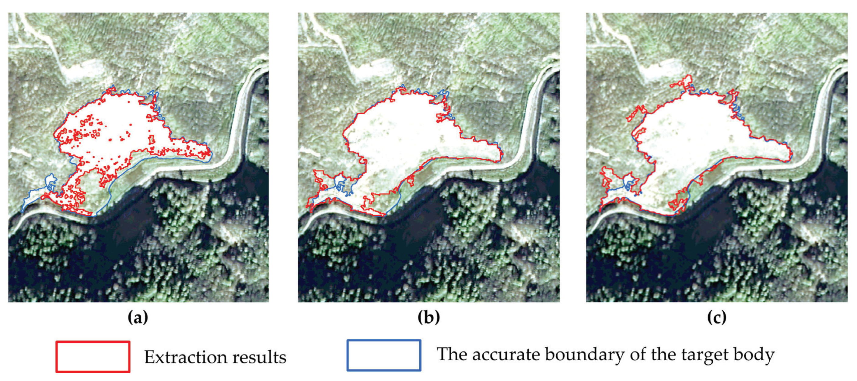
5.5. Extraction Accuracy

The area of the target body was extracted from the experimental image extraction information and the benchmark data area obtained from visual interpretation, and MLC, OOC, and Luv-RMWS methods δ_A were calculated using Equation (16). Meanwhile, the experimental image extraction information and benchmark data were divided into target and non-target objects. The number of pixels was used as the measurement unit, and the reference data of the target object was rasterized as the reference map. Then, the reference map was superimposed on the target segmentation results of the three methods to obtain the numbers of correctly and incorrectly segmented pixels. Equation (17) was used to calculate the δ_P values of the segmentation result, and the obtained results are shown in

Table 4. Evaluation of accuracy of unstable slope boundary extraction from experimental images.

Indicator	MLC	OOC	Luv-RMWS
${\delta }_A$	29.02%	8.71%	4.92%
${\delta }_P$	3.82%	1.90%	1.60%
$P_C$	96.18%	98.10%	98.40%
$P_{u_i}$	99.85%	94.06%	92.90%
$P_{A_j}$	71.03%	91.29%	95.08%
$K_{hat}$	80.93%	91.56%	93.05%

.

6. Discussion

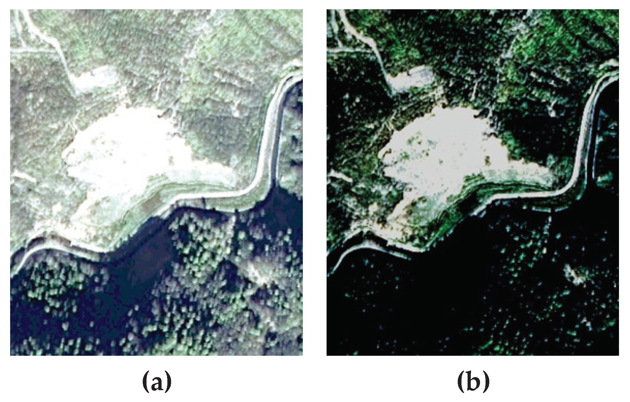
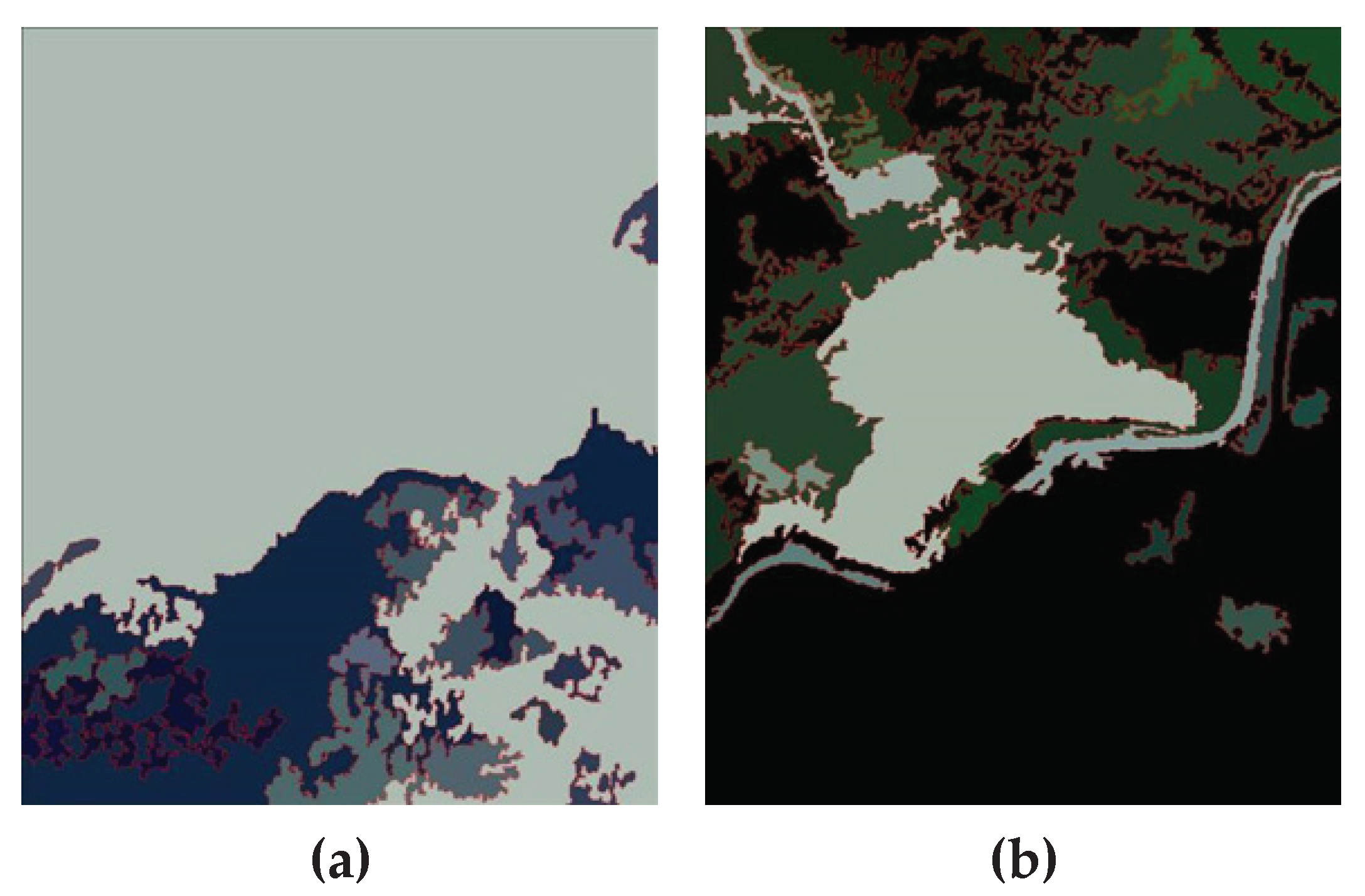
6.1. Analysis of Image Segmentation before and after Contrast Enhancement

It is observed from Figure 4 that the original image was severely under-segmented, and the target object, namely the unstable slope, failed to be extracted, while image contrast enhancement resulted in a good segmentation result, and the boundary of the extracted unstable slope body was highly consistent with the true boundary. The statistical results presented in Table 2 show that after image contrast enhancement, the number of image spots segmented by the watershed algorithm decreases rapidly, and the time consumption decreases slightly, thus achieving the goals of inhibiting over-segmentation and improving algorithm efficiency. Although the number of patches after region merging was increased compared to the original image data, time consumption was only half that of the original merging. Thus, the computational efficiency of the algorithm was greatly improved while obtaining good segmentation results. Therefore, the improvement due to contrast enhancement preprocessing on the image has a significant impact on the Luv-RMWS method and a significant effect on improving the segmentation efficiency and effect.

No pre-processing improvement was made to the algorithm described in this paper, with only contrast enhancement pre-processing performed on the original image data. Nevertheless, experiments show that increasing the image contrast leads to an improvement in the segmentation effect. In particular, when the original image was segmented, the unstable slope body could not be extracted due to the severe under-segmentation. Therefore, the contrast enhancement is an effective method for solving the problem of under-segmentation in the watershed segmentation algorithm. Nonetheless, the contrast enhancement in image pre-processing is usually subjective and random. In the future, the algorithm should be further improved by adding image contrast enhancement as the pre-processing step, and the effect of the algorithm should be improved by combining the "forward + post" improvements.

6.2. Analysis of Optimal Scale Parameters

A comparison of the multiscale Luv-RMWS slope hazard boundary segmentation test results with the visual segmentation results shows that the internal fragmented plots of the slope body increases with the gradual increase in C value, exhibiting over segmentation. As the D value gradually increases, the fragmented plots inside the slope body gradually decreases, and the extracted slope boundary stabilizes after D reaches 400. Based on a comparison of these results, the best target segmentation effect was obtained for C of 500 and D of 400, showing continuous borders, no freckles in the plaque, and a high degree of consistency with the shape of the target. Therefore, the optimal constant C for the minimum region decision threshold was set to 500, and the optimal value of the chromatic aberration value threshold D was set to 400.

The research was performed based on a GF-2 image, and the optimal segmentation and merging parameters were determined visually using a trial-and-error procedure. The optimal $C$ was 500 as determined by the minimum region A_min, while the optimal $D$ of chromatic aberration was 400. The test target had only one unstable slope in this paper. Therefore, the algorithm and program should be improved in subsequent research. The optimal decision thresholds for different image data and quality data should be determined, scale adaptive segmentation should be realized as much as possible, and rapid and automated remote sensing extraction of the slope hazard boundary should be achieved.

6.3. Analysis of Extraction Effect

As observed from Figure 6a and Figure 7a, the MLC method results were poor, and there were many fragments in the classification results, necessitating additional manual intervention for post-processing, so it is difficult to achieve automatic extraction. It is observed from Figure 6b,c that OOC and Luv-RMWS not only achieved better extraction of the target body but also combined fragmentation within the map spot, to obtain boundary extraction results of the unstable slope body with less interference from vegetation. However, as shown in Figure 7b,c, some over-segmentation and under-segmentation phenomena were still present; some large mis-segmented spots appeared at the trailing edge and bottom of the target, affecting the overall extraction effect.

An examination of the data presented in Table 3 shows that the MLC method required 381.000 s for extracting the target object, and the Luv-RMWS method required 39.702 s. The OOC method required merely 11.470 s, showing great time efficiency. It should be noted that the statistical time of MLC only specifies the time used for direct classification, and the classification result also contains many fragments that must be post-processed, which is an extremely time-consuming technical step. For this MLC test, the post-processing took more than 1 h. The comparison shows that OOC and Luv-RMWS carry out the splitter merger while completing the segmentation, and post-processing only converts raster data into vector data and makes a simple manual correction that requires no more than 0.5 h. Therefore, although the time efficiency of Luv-RMWS is slightly lower than OOC, it is much higher than MLC.

As observed from the data in Table 4, the δ_A and δ_P of the MLC method were 29.02% and 3.82%, and the δ_A and δ_P of OOC were 8.71% and 1.90%, both of which were larger than the δ_A (4.92%) and δ_P (1.60%) of Luv-RMWS, indicating that Luv-RMWS has higher extraction accuracy for an unstable slope boundary. At the same time, it can be seen from the P_C and K_hat that the Luv-RMWS method had the highest segmentation accuracy, followed by OOC, and the worst was MLC, which is consistent with the evaluation results of δ_A and δ_P [56,57], indicating that the evaluation criteria proposed in this paper are reliable.

6.4. Analysis of the Proposed Method

To date, many studies of landslide information extraction through image classification technology have been carried out [3,4,5,6]. SPOT 5, GF-1, ZY-3, and Unmanned Aerial Vehicle (UAV) images and other data have been often used as the data sources, while unsupervised and supervised classifications have been used as the technical means of performing the studies. In this paper, a GF-2 image was selected as the data source, and the MLC method was used for comparing the algorithm described in this paper. The performed experiments show that the Luv-RMWS method has obvious advantages regarding the information extraction time, avoids the complicated post-processing of MLC, and shows greatly improved time efficiency. Meanwhile, the initial segmentation results were automatically merged by Luv-RMWS, avoiding the subjectivity of artificially merging and processing fragments after MLC, and performed well in terms of comprehensive extraction efficiency and the objectivity of the extraction results.

Although current research in the field of image segmentation is based mostly on object-oriented multi-resolution segmentation methods [56,57], and the mature eCognition software is used as the test platform, the data are mainly concentrated in high-resolution remote sensing images such as GF-1, GF-2, and QuickBird. By contrast, the algorithm proposed in this paper does not need to establish the rules for the segmentation process, the merging process is simple, the algorithm is easy to understand, and the segmentation results are highly objective and reliable. The results of the multi-scale segmentation experiment using the proposed algorithm for extraction of the unstable slope boundary in experimental images show that Luv-RMWS performs well regarding the reliability of object extraction, the consistency of the object boundary, and the extraction details. Additionally, the calculated segmentation accuracy evaluation criteria show that the extraction results obtained by Luv-RMWS are more accurate, and the two accuracy factors used in this paper are superior to those obtained by the MLC and OOC methods. This is consistent with the results of visual evaluation and the results based on $P_C$, $P_{u_i}$, $P_{A_j}$ and $K_{hat}$, indicating that the evaluation criteria factor results for the image segmentation accuracy of the proposed watershed algorithm are reliable.

7. Conclusions

An improved watershed segmentation method (Luv-RMWS) is proposed for extracting slope hazard based on a high-resolution GF-2 remote sensing image. Additionally, the evaluation of extraction accuracy based on our proposed criteria of δ_A and δ_P is proven to be consistent with visual evaluation and a confusion matrix. It provides new accuracy evaluation indicators for evaluating the image watershed segmentation algorithm. The experimental results show the effectiveness of extracting the slope hazard boundary based on the Luv-RMWS. The post-improved Luv-RMWS algorithm was found to have a good effect in extracting slope hazard boundaries and a high time efficiency. It can obtain reliable and satisfying segmentation accuracy compared to MLC and OOC methods. Our methodology greatly improves the accuracy and processing time for slope hazards, and expands the application field of watershed segmentation algorithms.

References

1. Kalantar, B.; Pradhan, B.; Naghibi, S.A.; Motevalli, A.; Mansor, S. Assessment of the effects of training data selection on the landslide susceptibility mapping: A comparison between support vector machine (SVM), logistic regression (LR) and artificial neural networks (ANN). Geomat. Nat. Hazards Risk 2018, 9, 49–69. [Google Scholar] [CrossRef]
2. Peng, L.; Xu, S.N.; Mei, J.J.; Su, F.H. Earthquake-induced landslide recognition using high-resolution remote sensing image. J. Remote Sens. 2017, 4, 509–518. [Google Scholar]
3. Hervás, J.; Barredo, J.I.; Rosin, P.L.; Pasuto, A.; Mantovani, F.; Silvano, S. Monitoring landslides from optical remotely sensed imagery: The case history of Tessina landslide, Italy. Geomorphology 2003, 54, 63–75. [Google Scholar] [CrossRef]
4. Mondini, A.C.; Guzzetti, F.; Reichenbach, P.; Rossi, M.; Cardinali, M.; Ardizzone, F. Semi-automatic recognition and mapping of rainfall induced shallow landslides using optical satellite images. Remote Sens. Environ. 2011, 115, 1743–1757. [Google Scholar] [CrossRef]
5. Zhan, Z.Q.; Lai, B.H. A novel DSM filtering algorithm for landslide monitoring based on multi constraints. IEEE J. STARS 2015, 8, 324–331. [Google Scholar]
6. Zhang, M.M.; Xue, Y.A.; Li, J.; Shang, C.S. Identification of landslides and collapses based on remotely sensed imagery and DEM. Mine Surv. 2016, 44, 28–31. [Google Scholar]
7. Mohammad, D.H.; Chen, D.M. Segmentation for object-based image analysis (OBIA): A review of algorithms and challenges from remote sensing perspective. ISPRS J. Photogramm. 2019, 150, 115–134. [Google Scholar]
8. Vincent, L.; Soille, P. Watersheds in digital spaces: An efficient algorithm based on immersion simulations. IEEE Trans. Pattern Anal. Mach. Intell. 1991, 13, 583–598. [Google Scholar] [CrossRef] [Green Version]
9. Hagyard, D.; Razaz, M.; Atkin, P. Analysis of watershed algorithms for grey scale images. In Proceedings of the 3rd IEEE International Conference on Image Processing, Lausanne, Switzerland, 19 September 1996; Volume 3, pp. 41–44. [Google Scholar]
10. Shafarenko, L.; Petrou, M.; Kittler, J. Automatic watershed segmentation of randomly textured color images. IEEE Trans. Image Process. 1997, 6, 1530–1544. [Google Scholar] [CrossRef]
11. Smet, P.D.; Pires, R.L. Implementation and analysis of an optimized rain falling watershed algorithm. In Image and Video Communications and Processing International Society for Optics and Photonics; Proceedings of SPIE: San Jose, CA, USA, 2000. [Google Scholar]
12. Bieniek, A.; Moga, A. An efficient watershed algorithm based on connected components. Pattern Recogn. 2000, 33, 907–916. [Google Scholar] [CrossRef]
13. Soille, P. Morphological Image Analysis-Principles and Applications, 2nd ed.; Springer: Berlin, Germany, 2004; pp. 268–276. [Google Scholar]
14. Yu, Y.; Li, B.F.; Zhang, X.W.; Liu, Y.P.; Li, H.Q. Marked watershed segmentation algorithm for RGBD images. J. Image Graph. 2016, 21, 145–154. [Google Scholar]
15. Zhang, J.T.; Zhang, L.M. A watershed algorithm combining spectral and texture information for high resolution remote sensing image segmentation. Geomat. Inf. Sci. Wuhan Univ. 2017, 42, 449–455. [Google Scholar]
16. Yan, P.F.; Ming, D.P. Segmentation of high spatial resolution remotely sensed data using watershed with self-adaptive parameterization. Remote Sens. Technol. Appl. 2018, 33, 321–330. [Google Scholar]
17. Osma-Ruiz, V.; Godino-Llorente, J.I.; Sáenz-Lechón, N.; Gómez-Vilda, P. An improved watershed algorithm based on efficient computation of shortest paths. Pattern Recognit. 2007, 40, 1078–1090. [Google Scholar] [CrossRef]
18. Xiao, P.F.; Zhao, S.H.; She, J.F. Multispectral IKONOS image segmentation based on texture marker-controlled watershed algorithm. MIPPR 2007: Remote Sensing and GIS Data Processing and Applications and Innovative Multispectral Technology and Applications, International Society for Optics and Photonics, Wuhan, China, 2007. Int. Symp. Multispectr. Image Process. Pattern Recognit. 2007. [Google Scholar] [CrossRef]
19. Li, D.R.; Zhang, G.F.; Wu, Z.C.; Yi, L.N. An edge embedded marker-based watershed algorithm for high spatial resolution remote sensing image segmentation. IEEE Trans. Image Process. 2010, 19, 2781–2787. [Google Scholar]
20. Rizvi, I.A.; Mohan, B.K.; Bhatia, P.R. Multi-resolution segmentation of high-resolution remotely sensed imagery using marker-controlled watershed transform. In Proceedings of the International Conference and Workshop on Emerging Trends in Technology, Mumbai, Maharashtra, India, 25–26 February 2011. [Google Scholar]
21. Bala, A. An improved watershed image segmentation technique using MATLAB. Int. J. Sci. Eng. 2012, 3, 1–4. [Google Scholar]
22. Ng, H.P.; Ong, S.H.; Foong, K.W.C.; Goh, P.S.; Nowinski, W.L. Masseter segmentation using an improved watershed algorithm with unsupervised classification. Comput. Biol. Med. 2008, 38, 171–184. [Google Scholar] [CrossRef]
23. Xu, T.Z.; Zhang, G.C.; Jia, Y. Color image segmentation based on morphology gradients and watershed algorithm. Comput. Eng. Appl. 2016, 52, 200–203. [Google Scholar]
24. Chen, G. Image segmentation algorithm combined with regularized PM de-noising model and improved watershed algorithm. J. Med. Imaging Health Inform. 2020, 10, 515–521. [Google Scholar] [CrossRef]
25. Grau, V.; Mewes, A.U.J.; Alcaniz, M.; Kikinis, R.; Warfield, S.K. Improved watershed transform for medical image segmentation using prior information. IEEE Trans. Med. Imaging 2004, 23, 447–458. [Google Scholar] [CrossRef] [PubMed]
26. Li, B.; Pan, M.; Wu, Z.X. An improved segmentation of high spatial resolution remote sensing image using marker-based watershed algorithm. In Proceedings of the 20th International Conference on Geoinformatics, Hong Kong, China, 15–17 June 2012. [Google Scholar]
27. Xue, Y.A.; Zhang, M.M.; Zhao, J.L.; Guo, Q.H.; Ma, R. Study on quality assessment of multi-source and multi-scale images in disaster prevention and relief. Disaster Adv. 2012, 5, 1623–1626. [Google Scholar]
28. Wang, Y. Adaptive marked watershed segmentation algorithm for red blood cell images. J. Image Graph. 2018, 22, 1779–1787. [Google Scholar]
29. Jia, X.Y.; Jia, Z.H.; Wei, Y.M.; Liu, L.Z. Watershed segmentation by gradient hierarchical reconstruction under opponent color space. Comput. Sci. 2018, 45, 212–217. [Google Scholar]
30. Yasnoff, W.A.; Mui, J.K.; Bacus, J.W. Error measures for scene segmentation. Pattern Recognit. 1977, 9, 217–231. [Google Scholar] [CrossRef]
31. Dorren, L.K.A.; Maier, B.; Seijmonsbergen, A.C. Improved Landsat-based forest mapping in steep mountainous terrain using object-based classification. For. Ecol. Manag. 2003, 183, 31–46. [Google Scholar] [CrossRef]
32. Ming, D.P.; Luo, J.C.; Zhou, C.H.; Wang, J. Research on high resolution remote sensing image segmentation methods based on features and evaluation of algorithms. Geoinf. Sci. 2006, 8, 107–113. [Google Scholar]
33. Chen, Y.Y.; Ming, D.P.; Xu, L.; Zhao, L. An overview of quantitative experimental methods for segmentation evaluation of high spatial remote sensing images. J. Geoinf. Sci. 2017, 19, 818–830. [Google Scholar]
34. Huang, Q.; Dom, B. Quantitative methods of evaluating image segmentation. In Proceedings of the International Conference on Image Processing, Washington, DC, USA, 23–26 October 1995. [Google Scholar]
35. Jozdani, S.; Chen, D.M. On the versatility of popular and recently proposed supervised evaluation metrics for segmentation quality of remotely sensed images: An experimental case study of building extraction. ISPRS J. Photogramm. 2020, 160, 275–290. [Google Scholar] [CrossRef]
36. Debelee, T.G.; Schwenker, F.; Rahimeto, S.; Yohannes, D. Evaluation of modified adaptive k-means segmentation algorithm. Comput. Vis. Media 2019, 5, 347–361. [Google Scholar] [CrossRef] [Green Version]
37. Zhang, H.; Fritts, J.E.; Goldman, S.A. Image segmentation evaluation: A survey of unsupervised methods. Comput. Vis. Image Underst. 2008, 110, 260–280. [Google Scholar] [CrossRef] [Green Version]
38. Xiao, F.P. High Resolution Remote Sensing Image Segmentation and Information Extraction; Science Press: Beijing, China, 2012; pp. 151–156. [Google Scholar]
39. Zhu, C.J.; Yang, S.Z.; Cui, S.C.; Cheng, W.; Cheng, C. Accuracy evaluating method for object-based segmentation of high resolution remote sensing image. High Power Laser Part. Beams 2015, 27, 37–43. [Google Scholar]
40. Hoover, A.; Jean-Baptiste, G.; Jiang, X.Y.; Flynn, P.J.; Bunke, H.; Goldgof, D.; Bowyer, K.; Eggert, D.W.; Fitzgibbon, A.; Fisher, R. An experimental comparison of range image segmentation algorithms. IEEE Trans. Pattern Anal. Mach. Intell. 1996, 18, 673–689. [Google Scholar] [CrossRef] [Green Version]
41. Chen, H.C.; Wang, S.J. The use of visible color difference in the quantitative evaluation of color image segmentation. In Proceedings of the IEEE International Conference on Acoustics, Speech, and Signal Processing, Montreal, QC, Canada, 17–21 May 2004. [Google Scholar]
42. Hay, G.J.; Castilla, G.; Wulder, M.A.; Ruiz, J.R. An automated object-based approach for the multiscale image segmentation of forest scenes. Int. J. Appl. Earth Obs. Geoinf. 2005, 7, 339–359. [Google Scholar] [CrossRef]
43. Cardoso, J.S.; Corte-Real, L. Toward a generic evaluation of image segmentation. IEEE Trans. Image Process. 2005, 14, 1773–1782. [Google Scholar] [CrossRef] [Green Version]
44. Hofmann, P.; Lettmayer, P.; Blaschke, T.; Belgiu, M.; Wegenkittl, S.; Graf, R.; Lampoltshammer, T.J.; Andrejchenko, V. Towards a framework for agent-based image analysis of remote-sensing data. Int. J. Image Data Fusion 2015, 6, 115–137. [Google Scholar] [CrossRef] [Green Version]
45. Zhang, X.L.; Feng, X.Z.; Xiao, P.F.; He, G.J.; Zhu, L.J. Segmentation quality evaluation using region-based precision and recall measures for remote sensing images. ISPRS J. Photogramm. 2015, 102, 73–84. [Google Scholar] [CrossRef]
46. Wei, X.W.; Zhang, X.F.; Xue, Y. Remote sensing image segmentation quality assessment based on spectrum and shape. J. Geoinf. Sci. 2018, 20, 1489–1499. [Google Scholar]
47. Li, Z.Y.; Ming, D.P.; Fan, Y.L.; Zhao, L.F.; Liu, S.M. Comparison of evaluation indexes for supervised segmentation of remote sensing imagery. J. Geoinf. Sci. 2019, 21, 1265–1274. [Google Scholar]
48. Chen, L.F.; Liu, Y.M.; Liu, Y. Color image segmentation by combining improved watershed and region growing. Comput. Eng. Sci. 2013, 35, 93–98. [Google Scholar]
49. Lin, F.Z. Foundation of Multimedia Technology, 3rd ed.; Tsinghua University Press: Beijing, China, 2009; pp. 104–106. [Google Scholar]
50. Gao, W.; Xue, Y.A.; Zhao, J.L. Design and implementation of remote sensing image production quality quantitative evaluation system. J. Taiyuan Univ. Technol. 2014, 45, 776–779. [Google Scholar]
51. Hansen, M.W.; Higgins, W.E. Watershed-based maximum-homogeneity filtering. IEEE Trans. Image Process. 2002, 8, 982–988. [Google Scholar] [CrossRef] [PubMed]
52. Wei, D.F. There Search on the Methods of Landslide Edge Automatic Extraction Based on Remote Sensing Image. Master’s Thesis, Southwest Jiaotong University, Chendu, China, 2013. [Google Scholar]
53. Bruzzone, L.; Prieto, D.F. Unsupervised retraining of a maximum likelihood classifier for the analysis of multitemporal remote sensing images. IEEE Trans. Geosci. Remote Sens. 2001, 39, 456–460. [Google Scholar] [CrossRef] [Green Version]
54. Baatz, M.; Schäpe, A. Object-oriented and multi-scale image analysis in semantic networks. In Proceedings of the 2nd International Symposium on Operationalization of Remote Sensing, Enschede, The Netherlands, 16–21 August 1999. [Google Scholar]
55. Zhang, Y.J. A classification and comparison of evaluation techniques for image segmentation. J. Image Graph. 1996, 1, 151–158. [Google Scholar]
56. Huang, T.; Bai, X.F.; Zhuang, Q.F.; Xu, J.H. Research on Landslides Extraction Based on the Wenchuan Earthquake in GF-1 Remote Sensing Image. Bachelor Surv. 2018, 2, 67–71. [Google Scholar]
57. Li, Q.; Zhang, J.F.; Luo, Y.; Jiao, Q.S. Recognition of earthquake-induced landslide and spatial distribution patterns triggered by the Jiuzhaigou earthquake in 8 August 2017. J. Remote Sens. 2019, 23, 785–795. [Google Scholar]
Figure 1. Geographical map of the study area.
Ijgi 09 00246 g001
Figure 2. GF-2 remote sensing images: (a) original image and (b) contrast-enhanced image.
Ijgi 09 00246 g002
Figure 3. Flowchart of processing used in this paper.
Ijgi 09 00246 g003
Figure 4. Comparison of segmentation results between pre- and post-contrast-enhanced images.
Ijgi 09 00246 g004
Figure 5. Segmentation results of the slope hazard boundary using the multiscale Luv-RMWS.
Ijgi 09 00246 g005
Figure 6. Comparison of extraction of unstable slopes using the three methods: (a) MLC, (b) OOC, and (c) Luv-RMWS.
Ijgi 09 00246 g006
Figure 7. Comparison of extracted unstable slope using the three methods: (a) MLC; (b) OOC, and (c) Luv-RMWS.
Ijgi 09 00246 g007