Efficient Parallel K Best Connected Trajectory (K-BCT) Query with GPGPU: A Combinatorial Min-Distance and Progressive Bounding Box Approach

Abstract

Performing similarity analysis on trajectories consisting of massive numbers of tracking points is computationally challenging. We introduce a progressive minimum bounding rectangle (MBR) and minimum distance (MINDIST) approach to process the K Best Connected Trajectory (K-BCT) query, which aims to find the top K similarity trajectories to a given query trajectory. Our approach has three unique features to speed up the query. First, the approach builds a series of progressive MBRs from the query trajectory to determine the order of reference trajectories to identify the target top K reference trajectories at an earlier stage. Second, this method introduces a grid-based search method to speed up the matched point detection between two trajectories for similarity measures. Third, this approach further leverages the many-core computing power of Graphical Processing Unit (GPU) devices to perform the query in a parallel manner. We have conducted tests with ship tracking data and human movement data using GPU instances from Amazon Web Services. Preliminary results indicate that (a) parallel computing has greatly improved the efficiency of the query, and (b) our optimized approach can further speedup the computation compared to parallel implementations.

1. Introduction

With the development of location-based sensing techniques, trajectory datasets collected from different sensors have increased significantly [1]. A trajectory can describe the movements of vehicles, ships, species and other types of moving objects. It consists of a set of points collected from tracking devices (e.g., GPS devices). Performing spatiotemporal queries on those data becomes crucial in supporting various types of advanced analysis and decision-making [2]. Among those queries, identifying similar trajectories is one of the most popular query types because of its applications in numerous fields, such as identifying traffic congestions, summarizing human mobility patterns and planning for emergency routes [3]. Scientists have formulated various similarity measures according to the needs of specific domain applications [4]. Typical similarity measures include Euclidean Distance, Dynamic Time Warping and Hausdorff and Fréchet Distance [5].

Despite the variety of similarity measures, when performing similarity queries on massive trajectory datasets, scientists face computational challenges [6]. Examples of those challenges include how to perform similarity querying on trajectories consisting of massive tracking points in an efficient way and how to identify the targeted trajectories while reducing the number of the trajectories or tracking points to be checked to meet the memory constraints of devices. To address the computational challenges, previous studies have proposed optimization strategies [7] or parallel processing strategies that are implemented with either Graphical Processing Units (GPUs) or Central Processing Units (CPU) devices for handle a few selected types of similarity queries [8].

This paper describes a parallel approach to implement a type of similarity query—K Best connected trajectories (K-BCT) [9]. To our knowledge, our approach is the first parallel implementation solution to the K-BCT query. K-BCT query finds the trajectories that are close to a predefined trajectory. This query defines spatial closeness based on the concept of “One-way Distance” proposed by Lin and Su [10]. “One-way distance” is the weighted sum of the minimum distances from all points of one trajectory to another trajectory. According to Besse et al. [11], this distance measure can overcome some of the deficiencies of popular trajectory distance measures (e.g., Hausdorff Distance) in that it considers the shape and the physical location of trajectories. However, implementing this measure is computationally intensive. The distance computation alone has a level of complexity of O(n² log(n)) [11]. Therefore, an efficient processing strategy is necessary for the wide usage of the query.

Besides the inherent computational complexity of the K-BCT query, we are interested in this query because it involves three fundamental problems that widely exist in several spatiotemporal queries. First, this query calculates the shortest distance calculation from a point to a trajectory to measure similarity. Currently, GPU-based shortest distance calculation which computes the distances between all possible pairs of points and finds the smallest one among the distance values. The method has limited capabilities to handle massive trajectories [12]. Second, the K-BCT query includes different types of computations such as calculating distances on pairs of points of trajectories, deriving weighted sum of distance values of all points on a trajectory, and comparing similarity values derived from different trajectories (e.g., ranking similarity values of trajectories). The dependency of those computations introduces challenges in designing the parallel implementation strategies. Third, similar to other types of queries on massive data, the implementation of the K-BCT query includes a filtering step that identifies a set of candidate trajectories from a large number of trajectories to avoid unnecessary computation on all trajectories. Identifying the candidate set is part of the research question.

Our work makes the following contributions:

• We introduce an optimized and parallelizable processing workflow for the K-BCT query that integrates the concepts of progressive minimum bounding rectangles (MBRs), minimal distance (MINDIST) and uniform grid organization to speed up the execution of the query.
• We design and implement two levels of parallelisms: point level and trajectory level, to perform computationally intensive steps of the workflow in order to achieve performance gains and maintain spatial dependency of processing.

The rest of the paper is organized as follows: Section 2 reviews existing work in the field of similarity queries with a focus on using MBR and MINDIST to improve query processing. Section 3 describes the K-BCT query and our proposed optimized parallel approach to the query. Section 4 explains the experiments we have conducted to evaluate the approach. Summary and conclusion are given in Section 5.

2. Related Work

2.1. Computational Solutions to Similarity Queries

Identifying the similar trajectories to a given trajectory is a fundamental query type for trajectory data analysis [13]. Scientists have formulated different measures of the similarity for different purposes. To measure spatial similarity, geometric shape-based and directional-based similarity measures have been proposed (e.g., Hausdorff and Fréchet distances). To measure spatiotemporal similarity, time series-based and movement speed-based measures have been formulated (e.g., Time Warp Edit distance). The K-BCT query adopts the similarity measure based on the Euclidean distance and is an expansion of the point-based K Nearest Neighbor (KNN) query. Most of these measures have a high complexity and highly depend on the number of points of each trajectory to process. A complete review on different measures can be found in [13]. More recently, grid-based similarity measures that yield relatively low complexity have become popular [14]. Still, the computational intensity of implementing the similarity query on massive trajectory data often becomes a bottleneck [8,15]. Our goal is not to formulate a new similarity measure, but to design parallel solutions to support the execution of the query using the K-BCT query as an example.

The query processing on massive data usually takes a “filtering and refining” strategy [16,17]. The filtering stage identifies a set of trajectories from a large number of trajectories as candidate trajectories based on certain criteria (e.g., within a radius of a given trajectory). The trajectories in the set are sorted according to the criteria (e.g., the distances of trajectories to the given trajectory). The refining stage performs distance and similarity calculations on the sorted candidate trajectories to identify the final targeted ones. Scientists have formulated parallel computing approaches to address the computational limitations. Some efforts focus on formulating parallel computing strategies for the refining stage [18]. Those strategies group trajectories and perform queries on the multiple groups in a parallel manner. A few studies also examine how to identify the candidate trajectories [19].

To implement efficient parallel query processing, we propose optimizations for both the filtering and the refining stages. At the filtering stage, we identify the order of trajectories to be checked. At the refining stage, we focus on avoiding unnecessary computations. In particular, we aim to speed up the distance computation. Our optimization strategy is based on two major techniques: MBR and MINDIST to speed up the querying process.

2.2. MBR and MINDIST for Efficient Searching

MBR has been widely used in spatial database management and computational geometry as a typical strategy to organize, group and filter geometries [20]. MBR is the minimum bounding rectangle that encloses all parts of a given geometric feature. A MBR can be generated from any geometric feature such as a polyline or a multi-part polygon. Scientists have employed MBRs as a filtering method in the nearest neighbor (NN) search which identifies the nearest feature to a given feature [8]. MBR-based filtering process usually calculates the distances between the MBRs of features [17] (e.g., complex polygons) and sorts the features based on the distances. Because the distance computation is more efficient on MBRs, the filtering can quickly reduce the size of features for the fine level of computation.

While several studies have incorporated the concept of MBRs to improve the efficiency of similarity queries, most of existing researches produce one MBR for one trajectory and perform pruning checking using the MBRs of trajectories. In our research, we developed an enhanced version of MBRs, termed as “progressive MBRs”, to identify the candidate set of trajectories. Given the variety in shapes and patterns of a trajectory, one MBR of the entire trajectory does not provide a compact representation of the trajectory and thus provides less accurate filtering result [21]. Generating a series of MBRs using the sub-trajectories (or segments) of a trajectory can provide a more accurate depiction of the trajectory. To derive sub-trajectories, segmentation is necessary. Segmentation has been studied extensively in the context of trajectory representation. Segmentation partitions a trajectory into a series of segments or sub-trajectories and each segment is homogenous according to the segmentation criterion (e.g., direction) [22] of the segments to evaluate the overall patterns [23]. In this research, we utilize the concept of segmentation to build progressive MBRs for filtering.

In terms of the distance computation used for filtering and sorting, we incorporate the concept of minimum distances (i.e., MINDIST). MINDIST defines the minimum distance between the bounding rectangles of geometric objects. For example, MINDIST between two trajectories indicates that the distance between any pair of points from the two trajectories should be greater or equal to this distance. Since MBRs are bounding rectangles of trajectories, we can compute MINDIST between MBRs from trajectories and use the MINDIST as the measured values to rank the trajectories [24]. Besides providing measures for sorting trajectories, MINDIST can be used to terminate the search at an earlier stage. In the case of a NN search, when the distance between a pair of objects is smaller than the MINDIST of the rest objects, the pair of NN objects is found [8]. Therefore, we can use MINDIST to speed up the SD computation.

In this paper, we integrate MINDIST at the filtering and the refining stages. At the filtering stage, we calculate the MINDIST between the MBRs of trajectories and produce a list of sorted candidate trajectories based on the MINDIST. At the refining stage, we introduce a uniform grid indexing structure to decompose trajectories into grids and calculate the MINDIST between grids. With the MINDIST, we can sort the grids and perform distance computations between points within grids. The fine level of distance computation starts from the grids having the smallest MINDIST until we find the shortest distance. This feature allows us to avoid the distance computation for all possible pairs of points to speed up computation. To reduce the computational overhead as well as improving the processing efficiency, we propose novel parallel strategies to support the execution of the entire workflow

3. Methodology

3.1. K-BCT Query: Definition and Basic Implementation Procedure

K-BCT aims to find the most similar trajectories to a given query trajectory (Q) from a set of reference trajectories (R). Definition 1 describes the calculation of the similarity value [25].

Definition 1:

For a given trajectory Q = {$q_1,q_2,\dots q_m$} and a reference trajectory R = {$p_1,p_2, \dots , p_n$}, the distance is defined as:

$$Dist\left(q_i,R\right)=\underset{p_j\in i}{min}\left\{Dis{t}_e\left(q_i,p_j\right)\right\}$$

(1)

The similarity measure between Q and R is:

$$Sim\left(Q,R\right)=\sum _{i=1}^m{e}^{-Dis{t}_q\left(q_i,R\right)}$$

(2)

According to Definition 1, the larger the similarity value is, the more similar the two trajectories are. The K-BCT query ranks the similarity values of all possible pairs of Q and R to find the top K similar trajectories to Q. The execution of the query includes the following steps (Figure 1). The first step is to compute the distances between query points (q) and reference points (p). The second step is to identify the SD between q and R based on the distances from Step 1. The point on R corresponding to SD is identified as the “matched point” to q. To form a candidate set of R, for every q, the query finds the K nearest R based on all SD to q (denoted as Step 3 in Figure 1). The fourth step is to compute the similarity measures for all R in the candidate set. Finally, the query sorts the similarity measures in a descending order and returns the first K trajectories in the set.

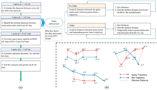
Figure 1. The workflow of K-BCT query: (a) major steps; (b) examples of identifying the matched points.

According to Figure 1, the K-BCT has five major steps. The table (Table 1) below summarizes the computational complexity of each step. n is the number of query points. m is the number of reference points. M is the number of reference trajectories. M’ is the number of reference trajectories from the KNN detection of points. m’ is the number of reference points from M’ trajectories. K is the number of reference trajectories to be identified.

Table 1. The complexity analysis of the major steps of K-BCT query.

Step	Serial Processing Complexity
1.Distance computation	O(n * m)
2.Shortest distance identification for query points	O(n * (m − M))
3.Point-based KNN trajectory identification	O(n * K * M’)
4.Similarity calculation using weighted sum of shortest distances	O(m’) + O(M’)
5.Trajectory-based KNN trajectory identification	O(K * M’)

Among the five steps, Step 2 is the most complex step as it involves order enforcements. The order constraint defines that the time stamp of the matched point of q_i from R should not be before the one of q_i−1. In Figure 2, Q consists of four points: q₁, q₂, q₃ and q₄. When the order constraint is effective, the matched points of query points can be different. Because p_1.2 is the matched point to q₂, to find the matched point of q₃, we should check the distances from q₃ to p_1.2, p_1.3, and p_1.4. Among those points, p_1.4 becomes the matched point to q₃. We define two different procedures to handle variations in order enforcement. When the order constraint is effective, for every point, we sort all distances to identify the matched point. When the order constraint is enforced, we introduce a “temporary point removal” mechanism. For every q, we store the matched point and temporarily remove all points before that point. In the next round, we only sort the distances associated the remaining points. In Figure 2, after we identify p_1.2 as the matched point to q₂, we remove p_1.1 from R₁ and sort the distances from p_1.2, p_1.3, and p_1.4.

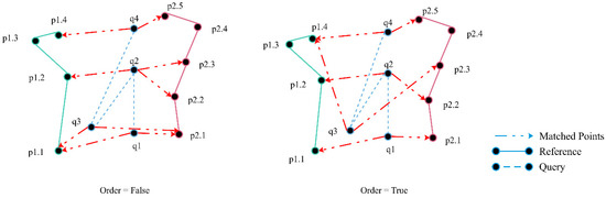
Figure 2. Enforcing the order constraint for shortest distance computation.

When applying the temporary point removal technique, users should specify the roles of trajectories (i.e., query trajectory and reference trajectory) as the roles can change the query results, especially when the order constraint is enforced. Given a pair of trajectories, assuming A is the query trajectory, the order of the points from A is used. The order of the matched points from B should follow the order of points on A. The results change when B is specified as the query trajectory. This issue is due to usage of the “One Way Distance” measure for similarity calculation. While other measures such as ones from the category of dynamic programming distances can address this issue, we follow the definition of the K-BCT query and plan to explore other measures in the future.

To implement the K-BCT in a parallel manner, we design two levels of parallel implementation: point level parallelism and trajectory level parallelism. Point level parallelism defines that every thread processes one or a set of points. This level of parallelism launches a large number of threads, achieving a high level of concurrency. Trajectory level parallelism defines that every thread processes one or a set of trajectories. Trajectory identification information is important in determining the results of the processing. Point and trajectory level parallelism apply to different steps of the K-BCT query (Table 2). For example, when the order constraint is enforced, every thread should record the order of the shortest distance points, and trajectory level of parallelism is appropriate. Besides the two levels of parallelism, we also incorporate the CUDA Thrust Library to perform the following operations: identify the unique trajectories, perform parallel transformations and sort the similarity values. The library provides parallel sorting methods (e.g., sort by value, sort by keys) and transformation methods to perform simple mathematical calculations. It also provides a range of complex data structures compared to the native CUDA libraries (e.g., the key value pair) with which we can perform data transfer between CPU and Thrust CUDA functions easily.

Table 2. Two types of parallelism: point and trajectory.

Parallelism	Number of Threads	Examples
Point	number of query points * number of reference points	Brute force distance computation (Step 1);
Trajectory	Number of query points * number of reference trajectories Or Number of query points * number of reference trajectories	Shortest distance computation (Step 2); Insert sorting to identify the smallest value in an array of value (Step 5);

To sum up, the parallel implementation revises the above procedure (Figure 1) in the following ways. The distance computation between every pair of points is conducted in a parallel manner (Step 1 in Figure 1). Every thread processes one pair of p and q. The SD identification differs with the enforcement of order constraint (Step 2 in Figure 2). In the case of no order constraint, every thread processes one q and one R to achieve trajectory level of parallelism. In the case of order constraint, every thread processes one Q and one R. Then, we perform a parallel sorting to identify the top K R to every q. Every thread processes one q and sorts the SD values from all R to q. We then use the unique function from the Thrust library to form a set of candidate trajectories with unique trajectory identifications (Step 3 in Figure 1). Finally, we develop a parallel transformation method to complete the computation of similarity values (Step 4 in Figure 1). Every thread transforms the distance values associated with one R to similarity values for the final step of sorting. Algorithm 1 describes the workflow of the parallel K-BCT query.

Algorithm 1 Parallel k-BCT: identify a top K similar trajectories in parallel

Input:

//A query trajectory includes an array of query points $Q=\left\{q_1,q_2,\dots ., q_m\right\}$

//A set of reference trajectories. Each trajectory has a list of points

$T=\left\{t_1, t_2, \dots , t_N\right\}$ //A list of reference points

$P=\left\{p_1, p_2, \dots , p_n\right\}$ $k$ //Integer, represents the amount of similar trajectories to be identified $order$ //Indicates if the order checking is enforced Output: $T_{top}$ //A list of top K similar trajectories 2DArray: $ED, SD, S{D}_k, PID, TI{D}_k$ //Compute the Euclidean distances $\mathrm{for}{q}_i \mathrm{in} Q \mathrm{do} \mathrm{in}\mathrm{parallel}$     $\mathrm{for}{t}_j \mathrm{in} T \mathrm{do} in parallel$        $\mathrm{for} p_x \mathrm{in} P \mathrm{do}$          $\mathrm{if}{p}_x\in t_j \mathrm{then}$            $ED\left[i\right]\left[x\right]=computeED\left(q_i, p_x\right)$

//Identify the top K similar trajectories

//from the every query point to every reference trajectory

$\mathrm{for}{t}_j \mathrm{in}T \mathrm{do} \mathrm{in}\mathrm{parallel}$     $\mathrm{if}\mathrm{order}\mathrm{then}$        $ID=-1$// Record the ID of the matched reference point        $\mathrm{for}{q}_i \mathrm{in} Q \mathrm{do}$          $dist=+\infty$          $\mathrm{for}{p}_x \mathrm{in} P \mathrm{do}$            $\mathrm{if} p_x\in t_j \mathrm{then}$              //x is the ID of the reference point              $\mathrm{if} ED\left[i\right]\left[x\right]<\mathrm{dist} \mathrm{and} ID\le x \mathrm{then}$                $\mathrm{dist}=ED\left[i\right]\left[x\right]$                $ID=x$          $SD\left[i\right]\left[j\right]=dist$          $PID\left[i\right]\left[j\right]=ID$          $\mathrm{insert}\mathrm{sort} dist to S{D}_k\left[i\right]$          $\mathrm{update} TI{D}_k\left[i\right]$ //$TI{D}_k$ holds the top k trajectory ID     else        $\mathrm{for}{q}_i \mathrm{in} Q \mathrm{do} \mathrm{in}\mathrm{parallel}$          $dist=+\infty , ID= -1$          $\mathrm{for}{p}_x \mathrm{in} P \mathrm{do}$            $\mathrm{if} p_x\in t_j \mathrm{then}$              $\mathrm{if} ED\left[i\right]\left[x\right]<\mathrm{dist} \mathrm{then}$ // No need to check ID                $\mathrm{dist}=ED\left[i\right]\left[x\right]$                $ID=x$          $SD\left[i\right]\left[j\right]=dist$          $PID\left[i\right]\left[j\right]=ID$          $\mathrm{insert}\mathrm{sort} dist to S{D}_k\left[i\right]$          $\mathrm{update} TI{D}_k\left[i\right]$ //$TI{D}_k$ holds the top k trajectory ID //Identify the unique trajectories as the candidate trajectories $TI{D}_k=\mathrm{unique}\left(TI{D}_k\right) \mathrm{in}\mathrm{parallel}$ //Calculate similarity Array: $sim, simID$ $\mathrm{for}j \mathrm{in} T_c \mathrm{do} \mathrm{in}\mathrm{parallel}$     $si{m}_j\leftarrow \mathrm{computeSim}\left(SD\left[i\right]\left[j\right]\right)$     $simID\leftarrow \mathrm{j}$ $\mathrm{sort}\mathrm{by}\left(sim, simID\right)$ $\mathrm{return} T\left(simID\left[0:k\right]\right) \mathrm{in}\mathrm{parallel}$

When the number of trajectories exceeds the limit of GPU onboard memory, the above parallel algorithm may not scale up to handle massive trajectories properly. To address the limitation of GPU memory, we perform the query with multiple rounds. Every round of querying processes a set of trajectories. At the end of every round, we compare the similarity values of the top K trajectories of the current round to the ones from previous rounds. Given the value of K is usually small (less than 100), this comparison is very efficient and does not require parallel processing. When multiple round of checking is necessary, if we can formulate a classification mechanism that group trajectories so that the targeted top K trajectories can be identified in the first few rounds, it is possible to terminate the search at an earlier stage. Therefore, creating a priority list of checking is important. Below we introduce the progressive MBR and MINDIST approach to identify the list.

3.2. Optimizations

3.2.1. Strategy 1: A Progressive MBR and MINDIST Based Filtering Method

As discussed in Section 2, we can rank the trajectories based on MINDIST calculated from MBRs. To create progressive MBRs, we introduce a two-step simplification and segmentation process. Simplification method is frequently used in the context of web-based visualization, which produces simplified representations of data at lower resolution levels. As the simplified representations include a subset of the original data, the processing time on the simplified representations can be reduced [26]. In our design, we apply the simplification algorithm to identify points that can partition the original trajectory rather than produce multi-resolution representations on the data because querying on simplified trajectories may introduce errors.

The two-step simplification and segmentation process is implemented as follows. First, we apply a variation-based simplification method [27] to remove the small variations and preserve the major characteristics of the trajectory. This method requires a minimum distance filter parameter (“error distance” in our method) as the input which adjusts the degree of simplification. The simplified trajectory consists of a set of points, termed as “anchor points”. Then, we apply a direction preservation segmentation method to break the simplified trajectory into multiple segments. The start and the end points of segments are termed as “transitive points”. Those transitive points are used to partition the original trajectory. All points from the trajectories are kept. In this way, we can produce a series of MBRs that can present the shape in a compact way. The construction of progressive MBRs is applied to the query trajectory only to avoid significant computational overhead. We also build MBRs for all reference trajectories. In the future, we will explore the effectiveness of applying the method to reference trajectories.

Figure 3 shows the process of producing progressive MBRs and filtering reference trajectories with MBRs. The original trajectory consists of a large set of points. After line simplification, anchor points are created for segmentation (Figure 3a). Transitive points break the original trajectory into three parts, and each part has a MBR (Figure 3b). The filtering is applied to the three MBRs of the query trajectory and the MBRs of reference trajectories (Figure 3c). In the case of using progressive MBRs, Trajectory 2 and 4 are not identified as intersecting trajectories to reduce the number of candidate trajectories.

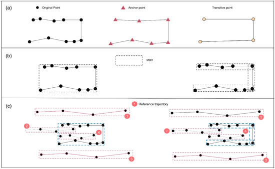
Figure 3. The process of producing progressive MBRs and filtering reference trajectories with MBRs: (a) line simplification and angular-based segmentation; (b) MBR creations; (c) intersection detection with different MBRs.

To integrate the MBR with the filtering stage, we compute the MINDIST and sort the reference trajectories by the MINDIST. Existing studies [17,28] in the field of spatial databases have adopted the concepts of MINDIST and MBR to form a pruning strategy which groups trajectories into two categories. Similarly, we classify the trajectories into two groups based on whether the MINDIST value is 0 or not. However, the second group is an ordered group. We introduce a two-phase checking method. At Phase 1, we compute the similarity values for all trajectories in Group 1 and keep top K similar trajectories only. At Phase 2, we compute the “maximum similarity value” (MSV) of unchecked trajectories and compare the value to the similarity values of the top K trajectories. If all similarity values in the candidate set are greater than the MSV, the search process is terminated. Otherwise, we continue to load trajectories in the candidate set, and repeat the similarity computation and comparison. The MSV value will be recomputed using the rest of unchecked trajectories that have not been checked. Not all trajectories in Phase 2 are subjected to similarity checking due to the enforcement of the maximum similarity value constraint. See Appendix B for the proof of checking.

Definition 2:

The maximum similarity value (MSV) of the unchecked trajectories is:

$$MSV=\sum _{i=1}^m{e}^{-min(MD\left(MBR\left(q_i\right), MBR\left(R_j\right)\right)}, i\in \left[1,m\right], j\in \left[n_1+1,n_2\right]$$

(3)

where:

• i is the ID of the query point
• m is the total number of query points from the query trajectory
• n₁ is the number of checked trajectories
• n₂ is the number of total trajectories
• MBR(q_i) is the progressive MBR corresponding to the query point i
• MBR(R_j) is the MBR corresponding to the unchecked reference trajectory j
• MD is the MINDIST from the progressive MBR containing a query point to the MBR of an unchecked reference trajectory.

Figure 4 shows an example of two-phase checking. Three progressive MBRs are available for the query trajectory. Trajectories in Group 1 are denoted as grey boxes. The MINDIST value of those trajectories are all 0. At Phase 1, we calculate the similarity values for R1, R2, R3, R5, R6, and R7 and sort the similarity values in a descending order. If K is 5, we only keep the top five trajectories. At Phase 2, we compute calculate the MSV using R4, R8 and R9 in the first round. If MSV is smaller than any of the similarity values among the top K trajectories from Phase 1, we terminate the search and return the top five trajectories. Otherwise, we then compute the similarity values of R4, R8, R9 and R10 and compare the similarity values to the ones from the top K trajectories.

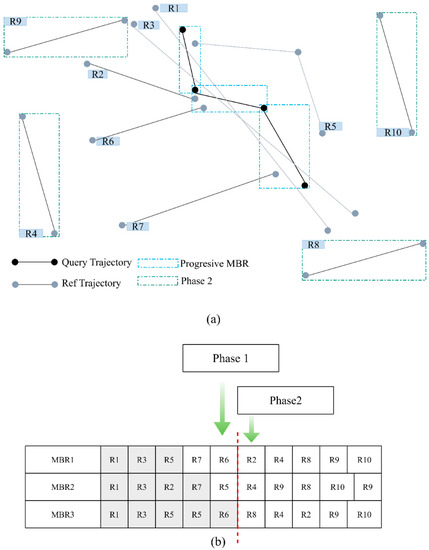
Figure 4. An example of selecting trajectories for Phase 1 and Phase 2 checking. (a) Spatial locations of trajectories; (b) sorted arrays for checking. Grey cells represent MINDIST = 0. For Phase 1, the unique trajectories are R1, R2, R3, R5, R6 and R7 (any trajectories with MINDIST = 0). For Phase 2, R2 is not included because the trajectory is checked in Phase 1. The unique trajectories in Phase 2 are R4, R8, R9 and R10.

Algorithm 2 describes the process of generating two lists of trajectories for the two-phase checking. The algorithm first performs line simplification on the query trajectory to identify a set of anchor points and builds a simplified trajectory with those anchor points (${\mathrm{Q}}_{\mathrm{c}}$). Then, it calculates the angles for every pair of consecutive points and determines the transitive points (${\mathrm{Q}}_{\mathrm{tr}}$). A segmentation process is started. Those transitive points are used to split the original trajectory and form sub-trajectories (${\mathrm{T}}_{\mathrm{seg}}$). Then, we build MBRs for every sub-trajectory or sub-segment as a series of progressive MBRs (${\mathrm{MBR}}_{\mathrm{q}}$) and the MBRs for every reference trajectories (${\mathrm{MBR}}_{\mathrm{p}}$). We further calculate the distances between MBRs (${\mathrm{SD}}_{\mathrm{MD}}$) and sort the reference trajectories (${\mathrm{TID}}_{\mathrm{MD}}$) by distances. With the distance information, we can identify the trajectories for Phase 1 and Phase 2 checking respectively. Algorithm 1 is first applied to the trajectories in Phase 1 and then applied to the trajectories in Phase 2.

Algorithm 2 Progressive MBR based MINDIST search

Input:

//A query trajectory includes an array of query points. $Q=\left\{q_1,q_2,\dots ., q_m\right\}$

//A set of reference trajectories. Each trajectory has a list of points.

$T=\left\{t_1, t_2, \dots , t_N\right\}$ //A list of reference points

$P=\left\{p_1, p_2, \dots , p_n\right\}$ $error$// Minimum distance filter parameter used in Douglas & Peucker algorithm Output:

$TI{D}_{MD}$ //Sorted IDs of trajectory lists $S{D}_{MD}$ //Sorted MINDST array Array: $MB{R}_q, MB{R}_p, Q_{tr}$ $Q_c= DQSimplify\left(Q, error\right)$ //Douglas & Peucker algorithm $\theta =0$ //Identify transitive points $\mathrm{for}\mathrm{every}\mathrm{pair} q_{ci}, q_{ci+1} \mathrm{in}{Q}_c \mathrm{do}$     ${\theta }_i= calculateDirection\left(q_{ci}, q_{ci+1} \right)$     $\mathrm{if}\left|{\theta }_i-\theta \right|>\frac{\pi }{4}\mathrm{and}\theta \ne 0 \mathrm{then}$        $Q_{tr}\leftarrow q_{ci}$    $\theta = {\theta }_i$ //Perform trajectory segmentation to produce a list of sub-trajectories $T_{seg}=segmentation\left(Q, Q_{tr}\right)$ //Calculate the MBRs for every sub trajectory $\mathrm{for}{t}_{seg} \mathrm{in}{T}_{seg} \mathrm{do} \mathrm{in}\mathrm{parallel}$     $MB{R}_q\leftarrow calculateMBR\left(t_{seg}\right)$ //Calculate the MBRs for every trajectory $\mathrm{for}{t}_i \mathrm{in}T \mathrm{do} \mathrm{in}\mathrm{parallel}$     $MB{R}_p\leftarrow calculateMBR\left(t_i\right)$ $\mathrm{for}i=0 \mathrm{to}count\left(MB{R}_q\right) \mathrm{do} \mathrm{in}\mathrm{parallel}$    $\mathrm{for}j=0 \mathrm{to}count\left(MB{R}_p\right) \mathrm{do} \mathrm{in}\mathrm{parallel}$       $S{D}_{MD}\left[i\right]\left[j\right]=calculateDis\left(MB{R}_{qi}, MB{R}_{pj}\right)$       $TI{D}_{MD}\left[i\right]\left[j\right]=j$       $sort by key \left(S{D}_{MD}\left[i\right], TI{D}_{MD}\left[i\right]\right)$ Array: $T_{\gamma }$ //Phrase 1 list Array: $T_{\beta }$ //Phrase 2 list $\mathrm{for}j=0 \mathrm{to}count\left(MB{R}_p\right) \mathrm{do}$     $coun{t}_{MD}=0$     $\mathrm{for}i=0 \mathrm{to}count\left(MB{R}_q\right) \mathrm{do}$        $\mathrm{if} S{D}_{MD}\left[i\right]\left[j\right]<0 \mathrm{then}$          $\mathrm{if} TI{D}_{MD}\left[i\right]\left[j\right] \notin T_{\gamma } \mathrm{then}$            $T_{\gamma }\leftarrow TI{D}_{MD}\left[i\right]\left[j\right]$

$\mathrm{else}$          $coun{t}_{MD}= coun{t}_{MD}+1$

$\mathrm{if} coun{t}_{MD}= coun{t}_{MBR}{}_q \mathrm{then}$        $T_{\beta }\leftarrow TI{D}_{MD}\left[i\right]\left[j\right]$

3.2.2. Strategy 2: A Grid-Based MINDIST Shortest Distance Search Method

To identify the shortest distance and the matched point for every query point, we introduce a parallel simple grid searching method [8] to speed up the shortest distance identification [14,15]. This idea is based on a few grid-based similarity measures (e.g., [20]). One popular grid-based similarity measure is proposed by Mariescu-Istodor and Fränti [14]. The measure produces gridded representations of trajectories. The similarity is measured based on the degree of overlapping cells of the grid representations from two trajectories. This approach avoids the expensive distance computation. Our approach also includes a grid construction process for trajectories (termed as “rasterization”). With the locational information of the grid cells, our approach performs distance computation on the grid cells to a query point to identify the grids that may contain the matched point to the query point and further compute the distances using all points in the grid to determine the matched point.

This method has the following features. First, it avoids distance calculation for all pairs of points to reduce the memory consumption and speed up the computation using a grid-based indexing structure. This method identifies the SD within a few rounds of distance comparison. Secondly, this method includes a parallel implementation of the grid indexing structure to reduce the additional computational overhead. Currently, only a few approaches have been proposed to implement parallel distributed indexing methods [29]. We choose the uniform grid indexing structure because the construction and data retrieval of such uniform structure are every efficient and the grid structure is highly independent and suitable for parallel implementation.

The method involves three major steps: (a) grid allocation and construction, (b) grid-based search, and (c) fine-level SD computation. At the first step, the method constructs a grid structure that overlays a matrix grid cells in the study area and computes grid coordinates to reference points. At the second step, the method calculates MINDIST between the progressive MBRs and the grid cells. The method sorts the grid cells based on the MINDIST values in an ascending order. At the third step, the method retrieves all points in the first grid cell of the sorted array, which has the smallest MINDIST, calculates the distances, and keeps the smallest distance only. If this distance is smaller than any of the MINDIST of the rest grid cells, the SD value and the matched point are found. Otherwise, the algorithm chooses the next grid in the array and repeats distance computation.

Figure 5 shows how the grid-based search method identifies the SD and the matched point. Given two trajectories, the rasterization process produces the gridded representation of the original trajectories. The rasterization process is similar to [14]. This method works well when points of the trajectory spread out in different grids. If all points of the reference trajectory are in the same grid cell, the method does not introduce any performance gains as all points are checked. Once the rasterization is completed, for a given query point, the search method calculates the MINDIST between the grid cells of the reference trajectory and finds the cell with the minimum MINDIST. The method then computes the distances between the query point and all points in the cell and finds the minimum distance. A special case is to handle the loops of trajectories when multiple points are in the same grid but with different time stamps. We strictly follow the definition of the K-BCT query and apply the temporal removal approach to determine the minimum distance point.

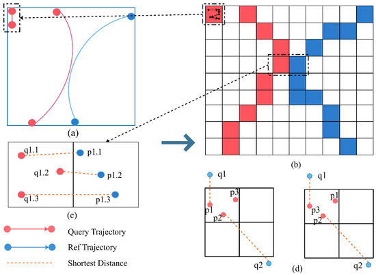
Figure 5. An example of the grid-based search method. (a) Original query and reference trajectories; (b) rasterized trajectory data; (c) distribution of query and reference points within grids and the matched point connection; (d) matched point connection when the order constraint is enforced.

Algorithm 3 describes the workflow. The algorithm requires the configuration of a uniform grid as an input parameter $\left(\mathrm{gd}\right)$. The configuration information includes the grid size and the spatial extent of the grid. A grid structure is also necessary to store the aggregated information from grid construction including the grid cells and the points in each of the grid cell $\left({\mathrm{G}}_{\mathrm{tj}}\right)$. For every reference point, the algorithm computes the grid locations $\left({\mathrm{g}}_{\mathrm{x}}\right)$. The calculation of grid locations is implemented in a parallel manner. Every thread computes the grid locations of a set of points. When the grid coordinates are computed, a serial post processing process aggregates points to grid cells $\left({\mathrm{G}}_{\mathrm{tj}}\right)$. When it comes to the SD computation for every pair of query point and reference trajectory, the algorithm first calculates the MINDIST $\left({\mathrm{MD}}_{\mathrm{tj}}\right)$ between the query point $\left({\mathrm{q}}_{\mathrm{i}}\right)$ and the grid cells $\left({\mathrm{g}}_{\mathrm{tj}}\right)$, sorts the grid cells and calcuates the distances between the query point and points in the grid cells. The order constraint changes the parallelism. If the order constraint is enforced, every thread processes one reference trajectory and the query trajectory. Otherwise, every thread processes a query point and a reference trajectory.

Algorithm 3 Grid MINDIST search method for the shortest distance computation

Input:

//A query trajectory includes an array of query points. $Q=\left\{q_1,q_2,\dots ., q_m\right\}$ //A set of reference trajectories. Each trajectory has a list of points. $T=\left\{t_1, t_2, \dots , t_N\right\}$ //A list of reference points

$P=\left\{p_1, p_2, \dots , p_n\right\}$ $\mathrm{gd}$//Grid configuration data structure, including grid size, grid extent Output:

$\mathrm{SD}$ // A list of the shortest distances

Initialize G

$\mathrm{for}{t}_j \mathrm{in}T \mathrm{do} \mathrm{in}\mathrm{parallel}$     Array: $G_{tj}$     $\mathrm{for} p_x \mathrm{in} P \mathrm{and} {\mathrm{p}}_{\mathrm{x}}\in t_j \mathrm{do} \mathrm{in}\mathrm{parallel}$        $g_x= calculateGridLoc\left(p_x, gd\right)$     //identify the list of grid locations for the trajectory     //and the number of points in every grid.     $G_t{}_j= aggregrate\left(g_x\right)$     $G\leftarrow G_t{}_j$

$\mathrm{for}{q}_i \mathrm{in}Q \mathrm{do}$     $\mathrm{for}{t}_j \mathrm{in}T \mathrm{do} \mathrm{in}\mathrm{parallel}$        Array: $M{D}_{tj}$        //Calculate the shortest distance between the grids and query point        $\mathrm{for} every g_{tj} \mathrm{in} G_{tj} \mathrm{do} \mathrm{in}\mathrm{parallel}$          $md=computeMINDIST\left(q_i, g_{tj}\right)$          $M{D}_{tj}\leftarrow md$          $GI{D}_{tj}\leftarrow g_{tj}$        $sort by key M{D}_{tj}, GI{D}_{tj}$ //$M{D}_{tj}$ is the key        $\mathrm{for} idx \mathrm{in} count\left(M{D}_{tj}\right) \mathrm{do}$          //Retrieve all points from the reference trajectory from the grid          $P_{tj}= getpoints\left(P, t_j, GI{D}_{tj}\left[idx\right]\right)$          //Compute the shortest distance between the query points          //and the reference points in the grid          $S{D}_{tj}= calculateSD\left(q_i, P_{tj}\right)$          //Terminate the loop          //when the SD is less than the next MD in the array          $\mathrm{if} {\mathrm{SD}}_{\mathrm{tj}}<M{D}_{tj}\left[idx+1\right] \mathrm{then}$            $\mathrm{break}$

3.3. Other Implementation Details

We have implemented all algorithms with NVIDIA GPUs. CUDA Toolkit 9.0 C++ version is the Software Development Kit (SDK) used for development to achieve the best efficiency of data processing. Any recent NVIDIA GPUs should support the execution of the algorithms. However, the maximum possible data processed by the algorithms are determined by the hardware configuration (e.g., the main memory and the memory GPU devices). Users can configure the number of trajectories to be processed per round to avoid memory issues. We have also implemented a serial version for comparison analysis.

4. Case Study

4.1. Test Datasets and Environments

We conduct three groups (denoted as “Group 1”, “Group 2”, and “Group 3” in later sections) of tests using datasets from three sources (Table 3). Appendix A provides detailed information about the test trajectories. Tests in Group 1 compare the performance of the serial processing and the parallel processing without applying two optimization strategies. Tests in Group 1 can demonstrate the performance gains of parallel processing on the K-BCT query. Tests in Group 2 and Group 3 evaluate the benefits of applying two optimization methods to speed up the computation and are conducted with our parallel version of the K-BCT query. Tests in Group 2 compare the performance differences with and without applying the progressive MBR-based sorting strategy. Tests in Group 3 compare the performance differences with and without the grid-based search method. In all groups, we record the time costs of running the query and analyze the additional time costs of implementing two optimization strategies. The test environment is an Amazon EC2 g3.4x large instance in the zone of US West (Oregon), equipped with one NVIDIA Tesla M60 GPU.

Table 3. Description of AIS [30], GeoLife [9] and Mopsi [14] datasets.

Dataset	Description	Spatial (Coverage)	Temporal (Frequency, Start and End Time)	Data Pattern
AIS: Ship tracks	Data collected from National Automatic Identification System provided by NOAA.	Vessel within U.S. coastal waters.	Data available from 2009 to 2014 at 1 min intervals.	Dataset has high density, trajectory/movements are not restricted in the open ocean.
Geolife: GPS tracks of citizens	GPS loggers and GPS-phones to collect trajectories from178 users.	Global	Every 1~5 s (2007–2011)	Dataset has high density, trajectories/movements are restricted by the underlying road network.
Mopsi: GPS tracks of citizens	Data collected with GPS-equipped devices from 51 users.	Global	Data collected between 2008 and 2014	Dataset has lower density and routes record activities such as hiking and biking.

4.2. Group 1: Serial Processing with CPU and Parallel Processing with GPU

Trajectories from the GeoLife dataset are used for comparisons between serial processing (with CPU) and parallel processing (with GPU). Three query trajectories containing 100, 200, and 300 points are selected. There are four groups of reference trajectories with 100, 300, 500, and 700 trajectories. In this test, we also evaluate the impacts of K and the order enforcement in altering the performances. K values of 5, 10, 15, and 20 are configured to find the top 5, 10, 15, and 20 similar trajectories for every query trajectories correspondingly. The speedup ratio is calculated (i.e., CPU calculation time (s)/GPU calculation time (s)). In all tests, the same query results are returned from serial processing and parallel processing.

According to Figure 6, using parallel processing has significantly improved the searching efficiency. The average speedup ratios are about 3296 (no order constraint) and about 1077 (with order constraint). Because reference trajectories have different number of points, the parallel processing may not maintain equalized workload distribution especially when the trajectory level parallelism is used. Besides the load imbalance issues, we identify three factors contributing to the variations in performances. First, speedup ratios increase significantly as the number of query points increases because the query execution gradually exploits full parallel computing capabilities. As the length of query trajectory increased from 100 to 300, the average speed up ratios increase from 1069 to 1122 with order constraint. Secondly, when enforcing the order constraint, the speedup ratio drops. The relatively lower speedup ratio is due to the fact that when enforcing the order constraint, the parallelism is trajectory-based. Third, when increasing the value of K, the speedup ratio tends to decrease, partly due to the larger number of trajectories that are recursively used in the sorting process. When the order constraint is enforced, the speedup ratio decreases slightly from 3559 to 3141 as K increases from 5 to 15.

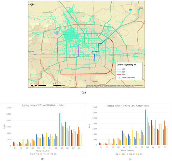
Figure 6. (a) Distribution of GeoLife query trajectories and reference trajectories data; (b) speedup ratios when there is no order constraint; (c) speedup ratios when there is order constraint.

4.3. Group 2: Integrating Progressive MBRs with the Parallel K-BCT Query

In this group of tests, we compare the performance differences when performing the K-BCT query in three cases: (a) no MBR applied, (b) one MBR, and (c) progressive MBRs with different simplification threshold values. In all cases, we use GPU parallel processing. The only difference is whether the MBR-based sorting strategy is applied. This set of tests uses ship tracking data collected in January 2014 in the zone of Universal Transverse Mercator (UTM) Zone 14. We summarize 9 different types of trajectories to gain a comprehensive view regarding how spatial characteristics of trajectories (e.g., spatial relationships between trajectories and the shapes of trajectories) can change the performance (Figure 7 and Figure 8). In terms of the shape characteristics of trajectories (Figure 7), we examine circular, significant transition (e.g., L-shaped), zigzag pattern and normal movements with local fluctuations. The relationship between the trajectories can be no intersection, a few intersections, intersections with multiple centers of reference trajectories, and highly mixed. We also consider the length of trajectories. While this is not an extremely comprehensive list, the test results should provide general gridlines regarding the applicability of the optimization method.

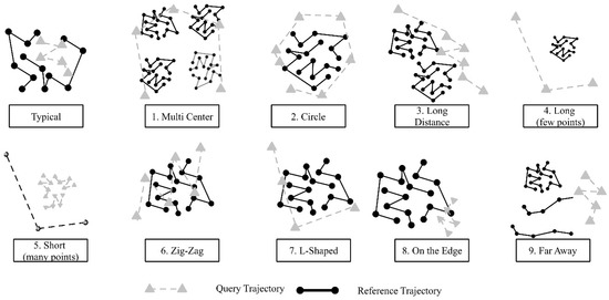
Figure 7. Different query trajectory patterns and shapes.

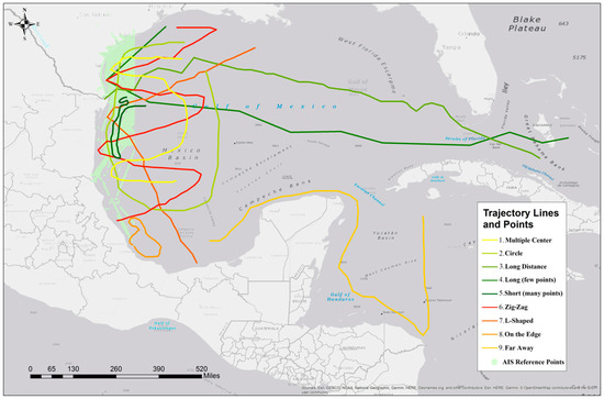
Figure 8. Distribution of query trajectories and points from reference trajectories.

We use 9 query trajectories with different shapes and patterns and 921 reference trajectories. To build the progressive MBRs, we choose different error distance values: 0.0001, 0.0005, 0.001, 0.005, 0.01 and 0.05 degrees to simplify the query trajectory. Different values may change the degree of simplification. K value is set as 20. Recall that this method applies when the data size is relatively large and multiple rounds of checking is necessary, we set the total rounds of checking to 23 and every round processes 40 trajectories. We record the time cost of performing K-BCT query to calculate speedup ratios, the total number of trajectories with overlapping MBRs and the number of trajectories checked. The percent of checked trajectories quantifies the reductions of the amount of trajectories for the refining stage. The tests are repeated with and without the order constraint.

In Figure 9, every trajectory has a set of seven records of performance measures. The first record corresponds with query execution when one MBR is used and the remaining six records represent the results of using progressive MBRs with six different error distances. Applying MBR-based priority checking can significantly improve the query efficiency. When the order constraint is not enforced, the speedup ratio of using one MBR and progressive MBRs ranges from 2.2 to 3.0. The average percent of trajectories intersected with MBRs is 71.1% with progressive MBRs and 80.2% with one MBR. The average percent of trajectories checked is 52.2% with progressive MBRs and 71.0% with one MBR. When the order constraint is effective, the average speedup ratios of using one MBR and progressive MBRs are 2.8 and 3.1. The progressive MBRs works extremely well in certain cases (e.g., Trajectory = 5, 8 and 9). In those cases, while the average percent of trajectories intersected remains the same (because order does not affect MBRs formation), the average percent of trajectories checked is 80.7% with one MBR and 71.3% with progressive MBRs. In both cases (with and without the order constraint), using different error distances for simplification changes the performance slightly. In most cases, the number of trajectories checked is highly correlated with the time cost of the query execution except for Trajectory 8. Even though the overall checked trajectories are the same for all cases, the priority lists could be different. Every round of processing is associated with a different level of load imbalance. We hope to address the load balance issue in the future. In all cases, the additional computational overhead (i.e., performing simplification, creating MBRs, computing MINDIST, and sorting MBRs based on MINDIST) counts less than 5% of the total time costs. Overall, using progressive MBRs can improve the query efficiency.

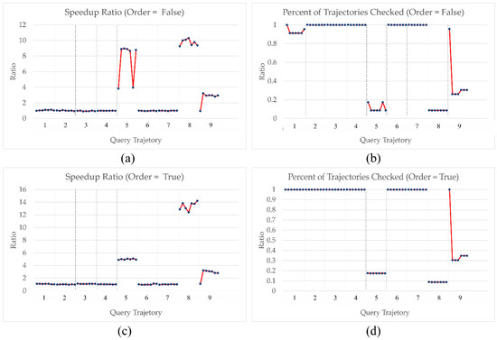
Figure 9. Comparing speedup ratio and percent of trajectories checked with using one MBR and multiple MBRs versus using no MBR applied. (a) Speedup ratios when there are no order constraints; (b) speedup ratios when there are order constraints; (c) the percent of reference trajectories checked when there is no order constraint; (d) the percent of reference trajectories checked when there is order constraint.

4.4. Group 3: Coupling Grid-Based MINDIST Search for SD Computation with the Parallel K-BCT Query

In this group of tests, we evaluate the performance change of using grid-based MINDIST search for SD computation. We again conduct the tests with the parallel version of the K-BCT query. The progressive MBR-based sorting strategy is applied to all tests. Given that all other factors remain the same, we can evaluate the role of the grid-based SD search method. We use the same reference dataset from Group 2 and a new dataset from Mopsi. For the AIS dataset, we select a group of six query trajectories (Group 3a) from the 921 reference trajectories. For the Mopsi data, we select a group of five query trajectories (Group 3b) from the 3107 trajectories located within Europe. The order enforcement is disabled in the Group 3 tests. We set up different grid sizes to examine the role of grid size in changing the performance. For Group 3a, four different grid sizes are used: 0.005, 0.01, 0.03, and 0.05 degrees. For Group 3.b, three different grid sizes are used: 0.01, 0.03, and 0.05 degrees. We record time cost to determine the speedup ratios. The construction time of the grid structure takes about 2% of the total processing time.

Figure 10a shows the distribution of selected query and reference trajectories. Figure 10b shows the speedup ratio. Among all trajectories, the average speedup ratio of 1.5. The highest speedup ratio is 2.5 and the lowest is 0.8. In a few cases, we do not observe performance gains. Grid size also affects the searching efficiency. For all 6 trajectories, the average speedup ratio is highest (1.76) when grid size is 0.05 degrees, and it is lowest (1.18) when grid size is 0.005 degrees. Figure 11a shows the distribution of selected query and reference trajectories. Figure 11b shows the speedup ratio. Among all trajectories, the average speedup ratio of 1.2. The highest speedup ratio is 1.4 and the lowest is 0.95. The speedup ratio is not as high as expected for three reasons. First, because the grid-based search method involves a lower level of parallelism with fewer threads can process data concurrently. This method is less capable of fully utilizing the parallel computational power of GPU cores. Secondly, computing the SD between grids and the query points is an additional step which introduces computational overhead. This computation is again performed with a lower level of parallelism. Finally, the process involves accessing the global memory and the shared memory from multiple query points which may introduce potential competition of memory access as well as a divergence issue of GPU.

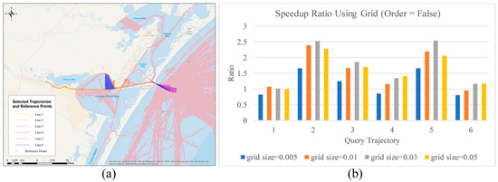
Figure 10. Comparing speedup ratio of AIS data (Group 3.a) using girds and without using grids: (a) The distribution of selected trajectories; (b) the comparison result.

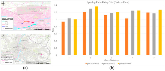
Figure 11. Comparing speedup ratio of Mopsi data (Group 3.b) using girds and without using grids: (a) The distribution of selected trajectories; (b) the comparison result.

4.5. Summary and Discussion

In summary, our approach introduces performance gains in all experiences. The speedup ratio is 3296 (without the order constraint) and 1077 (with the order constraint) with parallel processing comparing to serial processing respectively (Group 1). The results confirm that with the two levels of parallelism, our algorithm is extremely efficient for distance computations and sorting tasks. When the number of points exceeds the memory of GPU, two strategies are applied (Group 2 and Group 3).

When we use progressive MBRs to identify the priority of trajectories, we obtain a maximum speedup ratio of 3.0 (without the order constraint) and 3.1 (with order constraints) respectively compared to the basic parallel processing without applying any optimization strategies. Despite the performance gains, the spatial characteristics of trajectories can significantly affect the search efficiency. The optimization strategy works the best when the query trajectories have fewer points and are far away from the reference trajectories or clustered on the edge. In those cases, the MINDIST can clearly differentiate the most similar trajectories.

When we apply the grid-based searching strategy to SD computation, we obtain a maximum speedup ratio of 1.5 (without the order constraint) compared to the progressive MBRs search. This method works only with the low level of parallelism. Additional processing costs (e.g., grid construction, aggregation and sorting) as well as memory costs (e.g., accessing to the shared memory) become the bottlenecks of efficient computation. This pattern has been discussed in other literature as well. Results also show that the speedup ratio increases significantly by changing the grid size. Setting appropriate grid sizes can further optimize search efficiency. Constructing grids with larger cells takes less time but the search process tends to be longer because more points are assigned to every cell. In our tests, it is most efficient when the grid size is 0.03 degrees which balances the construction time and the searching time. In the future, we hope to explore solutions that can automatically identify an appropriate grid size based on the characteristics of data. For example, if trajectories differ significantly in spatial extents and lengths (e.g., Mospi dataset includes a few trajectories that are in a city whereas other trajectories that are in a country), the solution should be able to adjust the grid size based on such variations.

5. Conclusions and Future Work

In this paper, we report a parallel approach to implement the K-BCT query using many-core GPU techniques. The parallel implementation involves two major levels of parallelisms to handle the spatial dependency. This approach includes two additional optimization strategies to further improve query efficiency. According to the test results, our approach has significantly improved the efficiency of the query. Our parallel approach outperforms the conventional serial processing method. Nevertheless, the efficiency of the optimization strategies can be affected by factors such as the shapes and patterns of trajectories.

In the future, there are several options that can take this research to another level: (a) using MBRs from reference trajectories to identify the priority list and incorporating spatial tree-based indices such as R-tree or Quad-tree to better improve the filtering efficiency, (b) integrating the query method with real time streaming data and performing the query on-the-fly to support time critical analysis; (c) including a task redistribution method based on trajectory density or point density to achieve a balanced workload assignment among multiple computing threads; and (d) expanding the workflow to support other types of similarity queries

References

- Yuan, J.; Zheng, Y.; Zhang, C.; Xie, W.; Xie, X.; Sun, G.; Huang, Y. T-drive: Driving directions based on taxi trajectories. In Proceedings of the 18th SIGSPATIAL International Conference on Advances in Geographic Information Systems; ACM: New York, NY, USA, 2010; pp. 99–108. [Google Scholar]
- Zheng, Y. Trajectory data mining: An overview. ACM Trans. Intell. Syst. Technol. 2015, 6. [Google Scholar] [CrossRef]
- Tiakas, E.; Papadopoulos, A.N.; Nanopoulos, A.; Manolopoulos, Y.; Stojanovic, D.; Djordjevic-Kajan, S. Searching for similar trajectories in spatial networks. J. Syst. Softw. 2009, 82, 772–788. [Google Scholar] [CrossRef]
- Etienne, L.; Devogele, T.; Buchin, M.; McArdle, G. Trajectory Box Plot: A new pattern to summarize movements. Int. J. Geogr. Inf. Sci. 2016, 30, 835–853. [Google Scholar] [CrossRef]
- Magdy, N.; Sakr, M.A.; Mostafa, T.; El-Bahnasy, K. Review on trajectory similarity measures. In Proceedings of the IEEE 7th International Conference on Intelligent Computing and Information Systems (ICICIS), Cairo, Egypt, 12–14 December 2015. [Google Scholar]
- Deng, K.; Xie, K.; Zheng, K.; Zhou, X. Trajectory indexing and retrieval. In Computing with Spatial Trajectories; Springer: New York, NY, USA, 2011; pp. 35–60. ISBN 978-1-4614-1628-9. [Google Scholar]
- Frentzos, E.; Gratsias, K.; Theodoridis, Y. Index-based most similar trajectory search. In Proceedings of the IEEE 23rd International Conference on Data Engineering, Istanbul, Turkey, 15–20 April 2007. [Google Scholar]
- Gowanlock, M.; Casanova, H. Indexing of spatiotemporal trajectories for efficient distance threshold similarity searches on the GPU. In Proceedings of the IEEE International Parallel and Distributed Processing Symposium, Hyderabad, India, 25–29 May 2015. [Google Scholar]
- Zheng, Y.; Xie, X.; Ma, W.-Y. Geolife: A collaborative social networking service among user, location and trajectory. IEEE Data Eng. Bull. 2010, 33, 32–39. [Google Scholar]
- Lin, B.; Su, J. One way distance: For shape based similarity search of moving object trajectories. GeoInformatica 2008, 12, 117–142. [Google Scholar] [CrossRef]
- Besse, P.; Guillouet, B.; Loubes, J.-M.; François, R. Review and Perspective for Distance Based Trajectory Clustering. arXiv, 2015; arXiv:1508.04904. Available online: http://arxiv.org/abs/1508.04904 (accessed on 20 June 2018).
- Arefin, A.S.; Riveros, C.; Berretta, R.; Moscato, P. Gpu-fs-knn: A software tool for fast and scalable knn computation using gpus. PLoS ONE 2012, 7. [Google Scholar] [CrossRef] [PubMed]
- Wang, H.; Su, H.; Zheng, K.; Sadiq, S.; Zhou, X. An effectiveness study on trajectory similarity measures. In Proceedings of the Twenty-Fourth Australasian Database Conference-Volume 137; Australian Computer Society, Inc.: Darlinghurst, Australia, 2013; pp. 13–22. [Google Scholar]
- Mariescu-Istodor, R.; Fränti, P. Grid-based method for GPS route analysis for retrieval. ACM Trans. Spat. Algorithms Syst. 2017, 3. [Google Scholar] [CrossRef]
- Zhang, J.; You, S.; Gruenwald, L. U 2 STRA: High-performance data management of ubiquitous urban sensing trajectories on GPGPUs. In Proceedings of the 2012 ACM Workshop on City data Management Workshop; ACM: New York, NY, USA, 2012; pp. 5–12. [Google Scholar]
- Jacox, E.H.; Samet, H. Spatial join techniques. ACM Trans. Database Syst. 2007, 32. [Google Scholar] [CrossRef]
- Rahat, T.A.; Arman, A.; Ali, M.E. Maximizing reverse k-nearest neighbors for trajectories. In Databases Theory and Applications; Lecture Notes in Computer Science; Springer: Cham, Switzerland, 2018; pp. 262–274. [Google Scholar]
- Lettich, F.; Orlando, S.; Silvestri, C. Processing streams of spatial k-NN queries and position updates on manycore GPUs. In Proceedings of the 23rd SIGSPATIAL International Conference on Advances in Geographic Information Systems; ACM: New York, NY, USA, 2015. [Google Scholar]
- Leal, E.; Gruenwald, L.; Zhang, J.; You, S. Tksimgpu: A parallel top-k trajectory similarity query processing algorithm for gpgpus. In Proceedings of the IEEE International Conference on Big Data (Big Data), Santa Clara, CA, USA, 29 October–1 November 2015. [Google Scholar]
- Papadias, D.; Theodoridis, Y. Spatial relations, minimum bounding rectangles, and spatial data structures. Int. J. Geogr. Inf. Sci. 1997, 11, 111–138. [Google Scholar] [CrossRef]
- Tripathi, P.K.; Debnath, M.; Elmasri, R. A direction based framework for trajectory data analysis. In Proceedings of the 9th ACM International Conference on PErvasive Technologies Related to Assistive Environments; ACM: New York, NY, USA, 2016. [Google Scholar]
- Long, C.; Wong, R.C.-W.; Jagadish, H.V. Direction-preserving trajectory simplification. Proc. VLDB Endow. 2013, 6, 949–960. [Google Scholar] [CrossRef]
- Brox, T.; Malik, J. Object segmentation by long term analysis of point trajectories. In European Conference on Computer Vision; Lecture Notes in Computer Science; Springer: Berlin/Heidelberg, Germany, 2010; pp. 282–295. [Google Scholar]
- Zou, Y.-G.; Fan, Q.-L. OQ-Quad: An efficient query processing for continuous k-nearest neighbor based on quad tree. In Proceedings of the 4th International Conference on Computer Science & Education, Nanning, China, 25–28 July 2009. [Google Scholar]
- Chen, Z.; Shen, H.T.; Zhou, X.; Zheng, Y.; Xie, X. Searching trajectories by locations: an efficiency study. In Proceedings of the 2010 ACM SIGMOD International Conference on Management of Data; ACM: New York, NY, USA, 2010; pp. 255–266. [Google Scholar]
- Waga, K.; Tabarcea, A.; Mariescu-Istodor, R.; Fränti, P. Real time access to multiple GPS tracks. In Proceedings of the 9th International Conference on Web Information Systems and Technologies (WEBIST 2013), Aachen, Germany, 8–10 May 2013; pp. 293–299. [Google Scholar]
- Douglas, D.H.; Peucker, T.K. Algorithms for the reduction of the number of points required to represent a digitized line or its caricature. Cartographica 1973, 10, 112–122. [Google Scholar] [CrossRef]
- Kothuri, R.V.; Ravada, S. Pruning of Spatial Queries Using Index Root MBRS on Partitioned Indexes. U.S. Patent No. 7877405, 25 January 2011. [Google Scholar]
- Wang, H.; Belhassena, A. Parallel trajectory search based on distributed index. Inf. Sci. 2017, 388, 62–83. [Google Scholar] [CrossRef]
- MarineCadastre.gov|Vessel Traffic Data. Available online: https://marinecadastre.gov/ais/ (accessed on 6 June 2018).
© 2018 by the authors. Licensee MDPI, Basel, Switzerland. This article is an open access article distributed under the terms and conditions of the Creative Commons Attribution (CC BY) license (http://creativecommons.org/licenses/by/4.0/).