
Morphological Operations to Extract Urban Curbs in 3D MLS Point Clouds

 ,
,  and
and
Abstract
:1. Introduction
2. Related Work
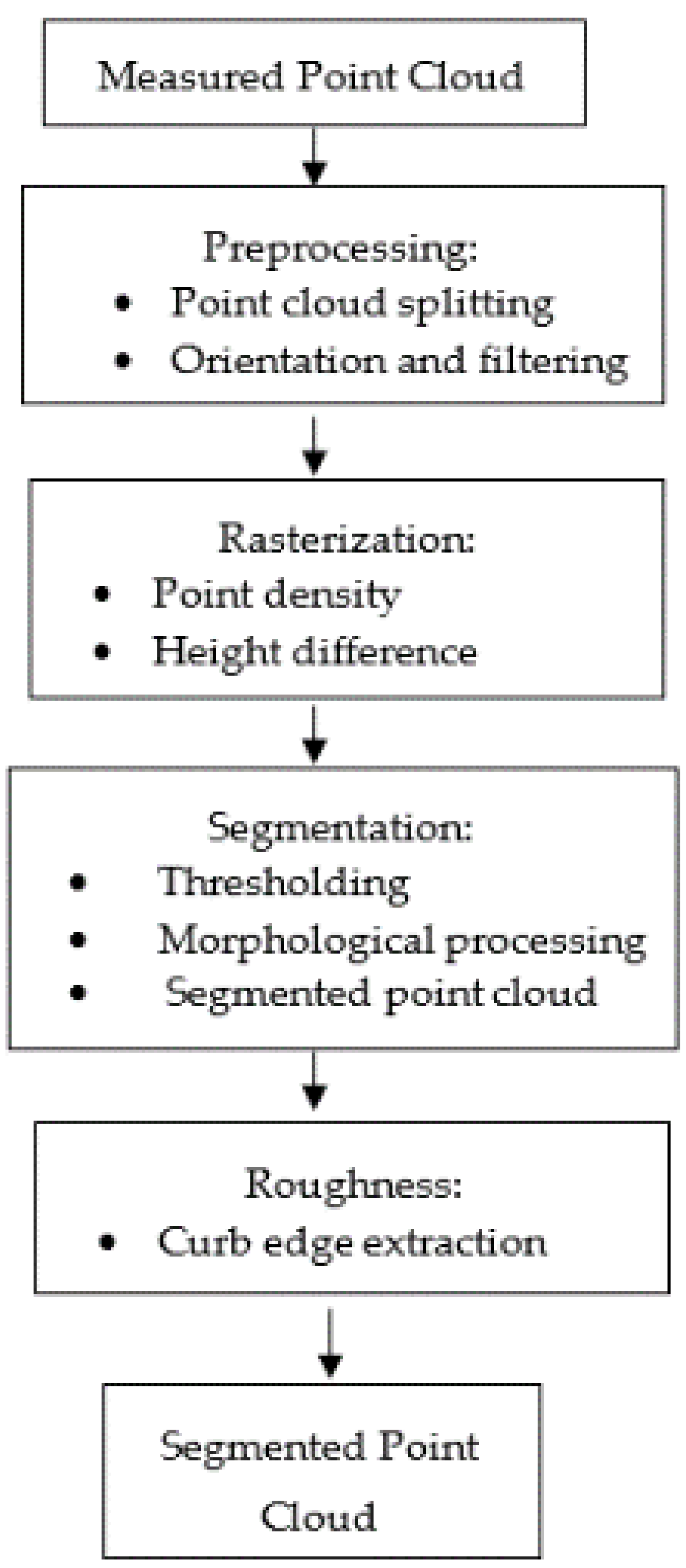
3. Methodology
3.1. Preprocessing
3.1.1. Point Cloud Splitting
3.1.2. Orientation and Filtering
3.2. Rasterization
3.3. Segmentation
3.3.1. Thresholding
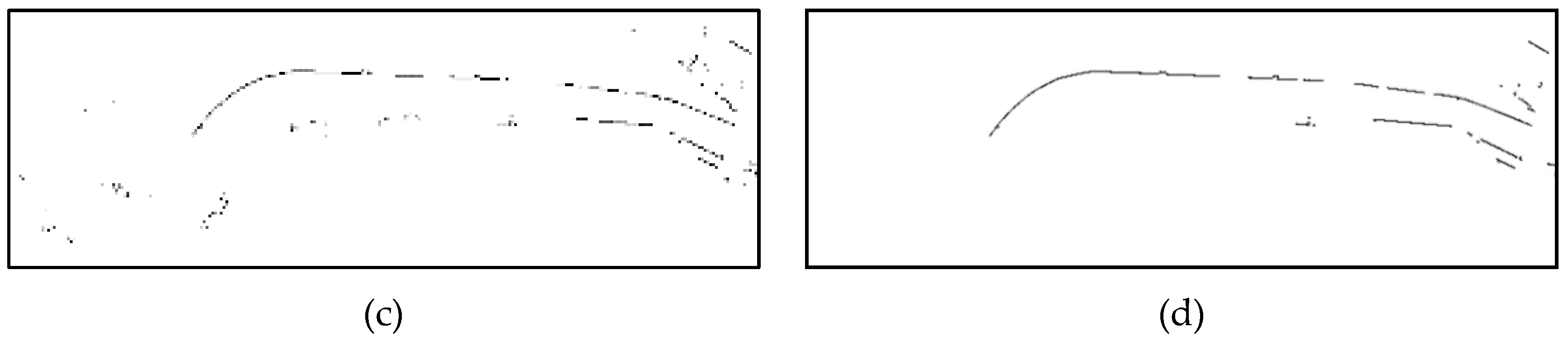
3.3.2. Morphological Operations
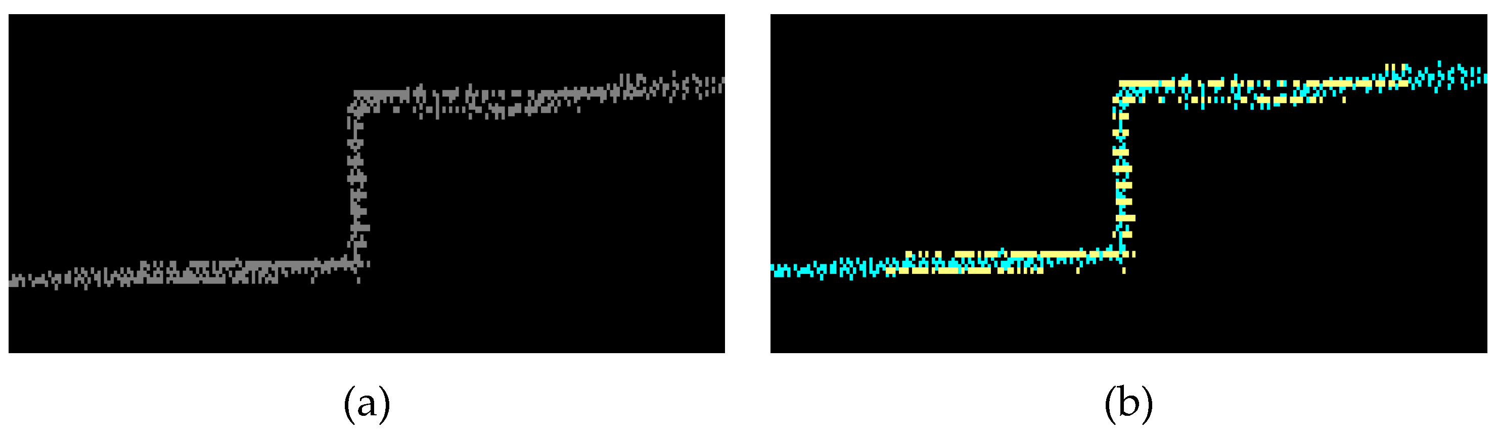
3.3.3. Segmented Point Cloud
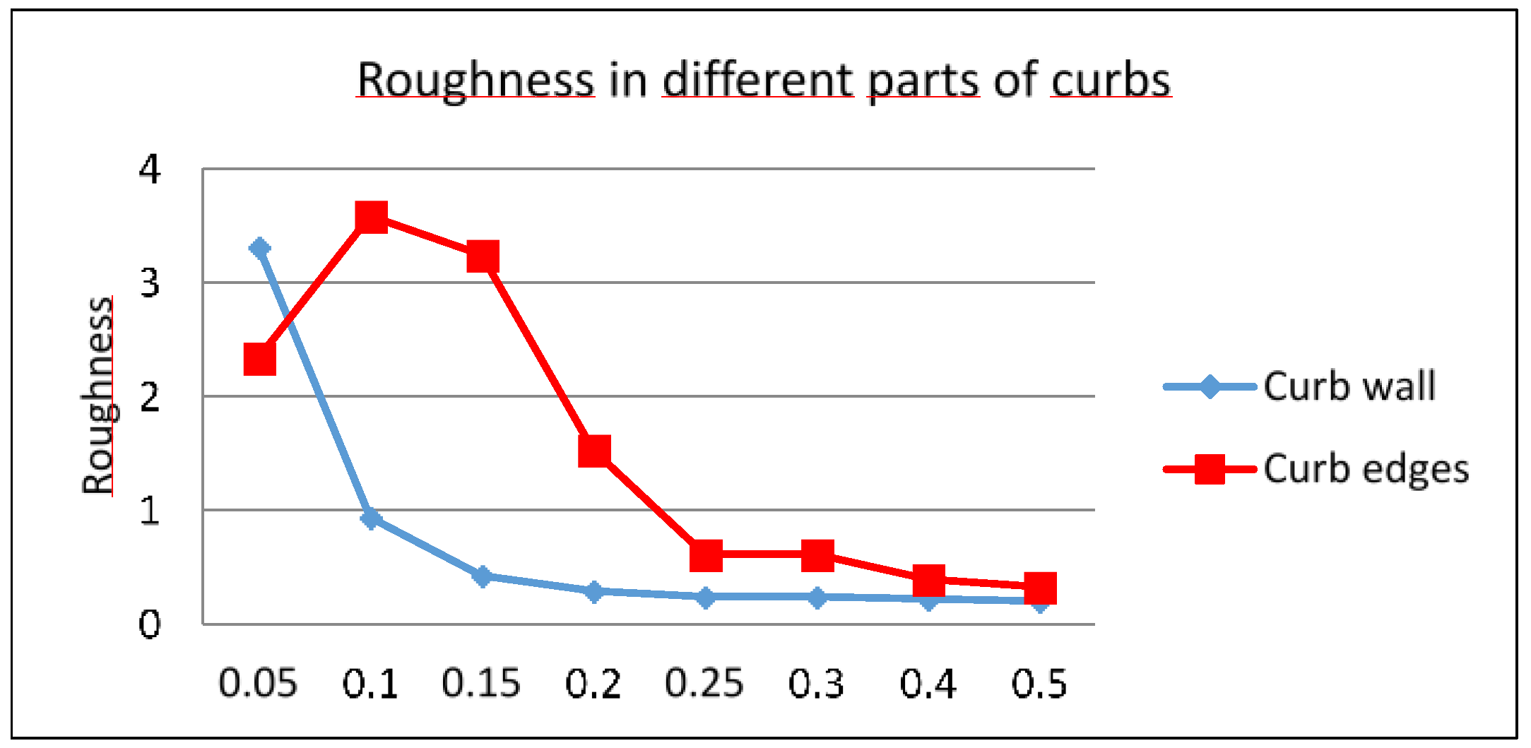
3.4. Roughness
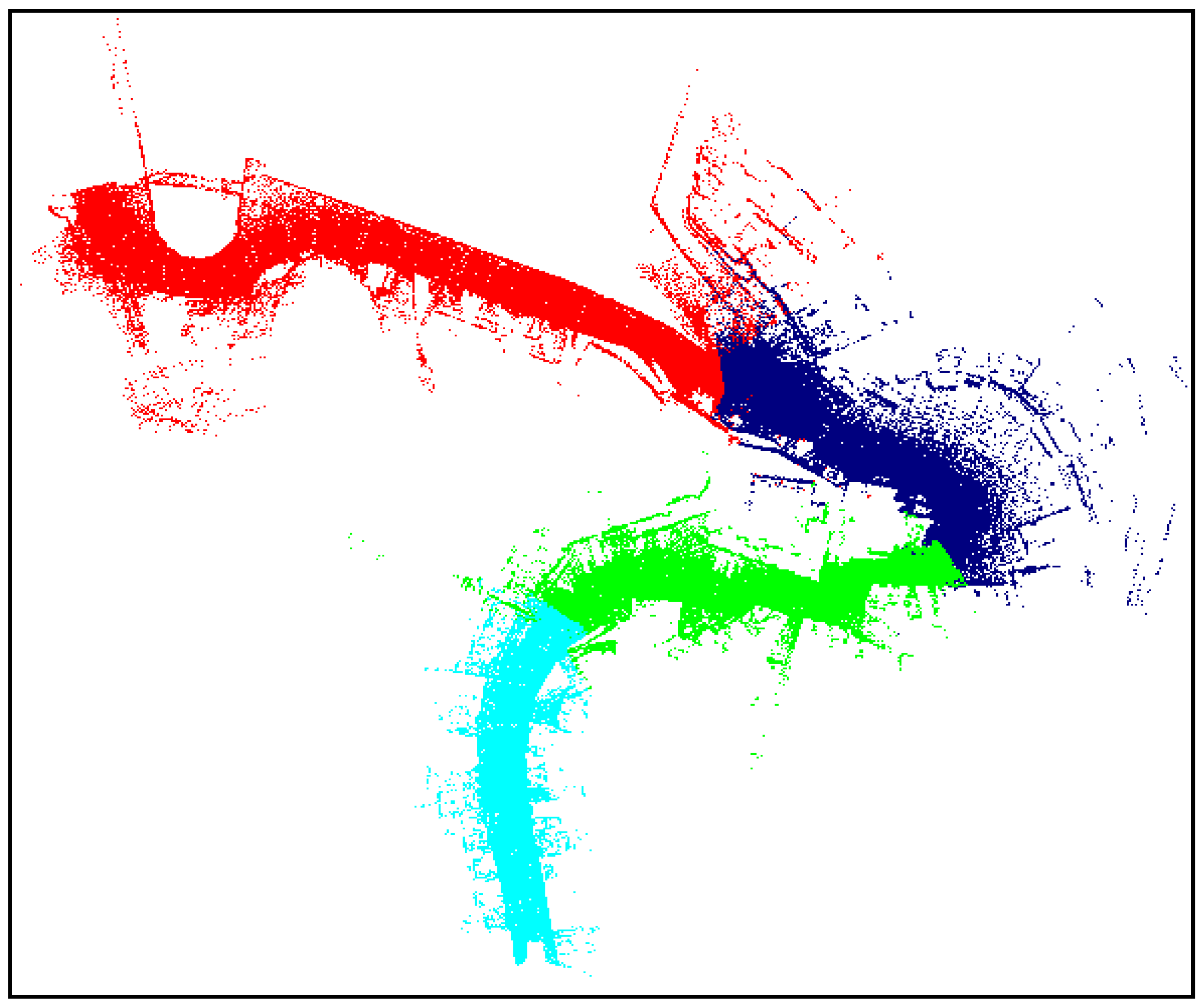
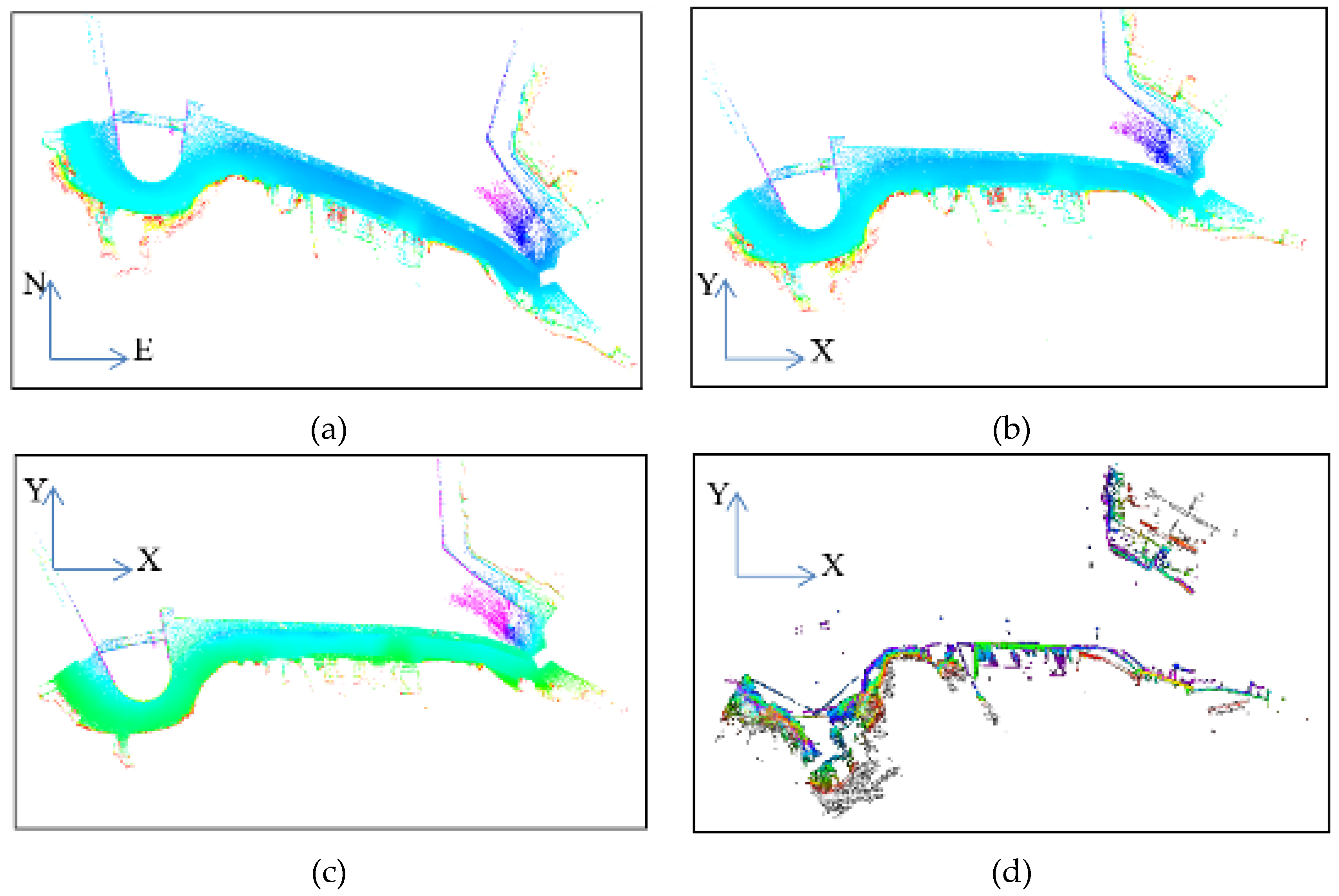
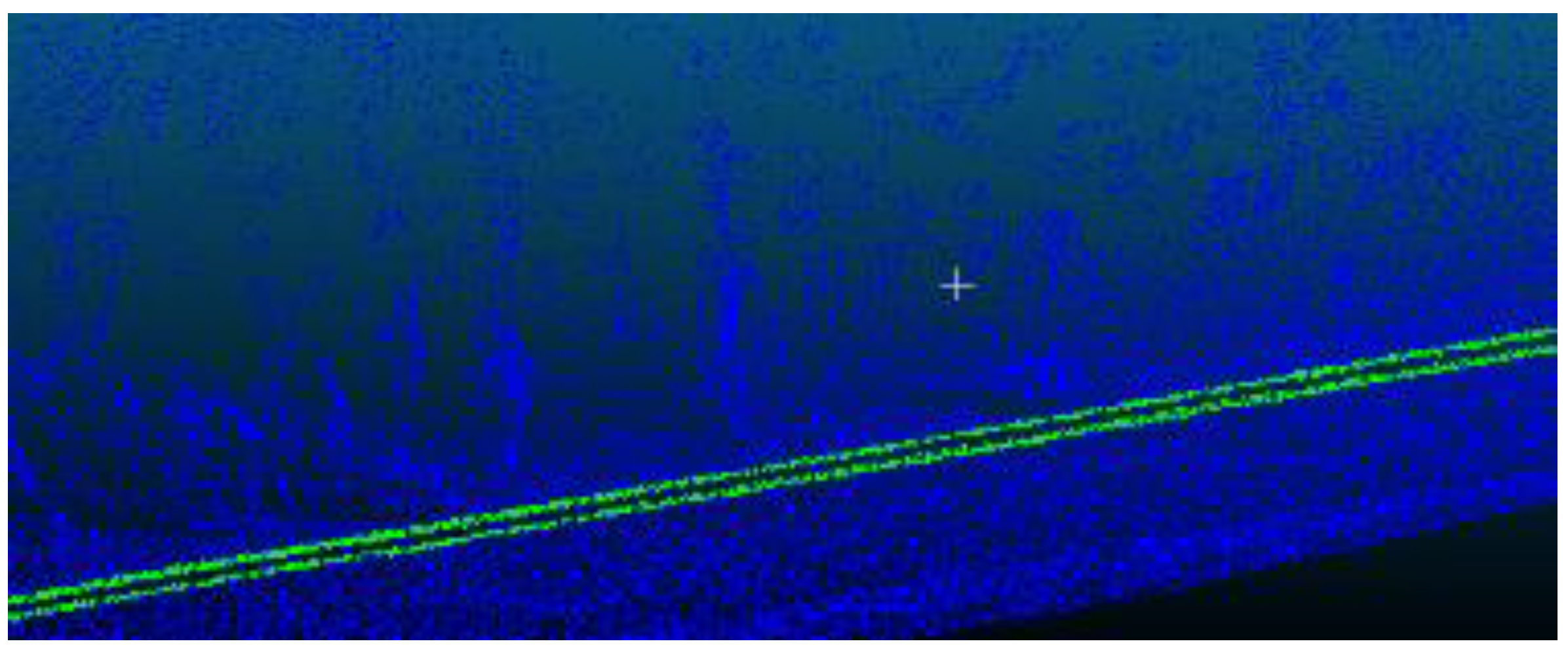
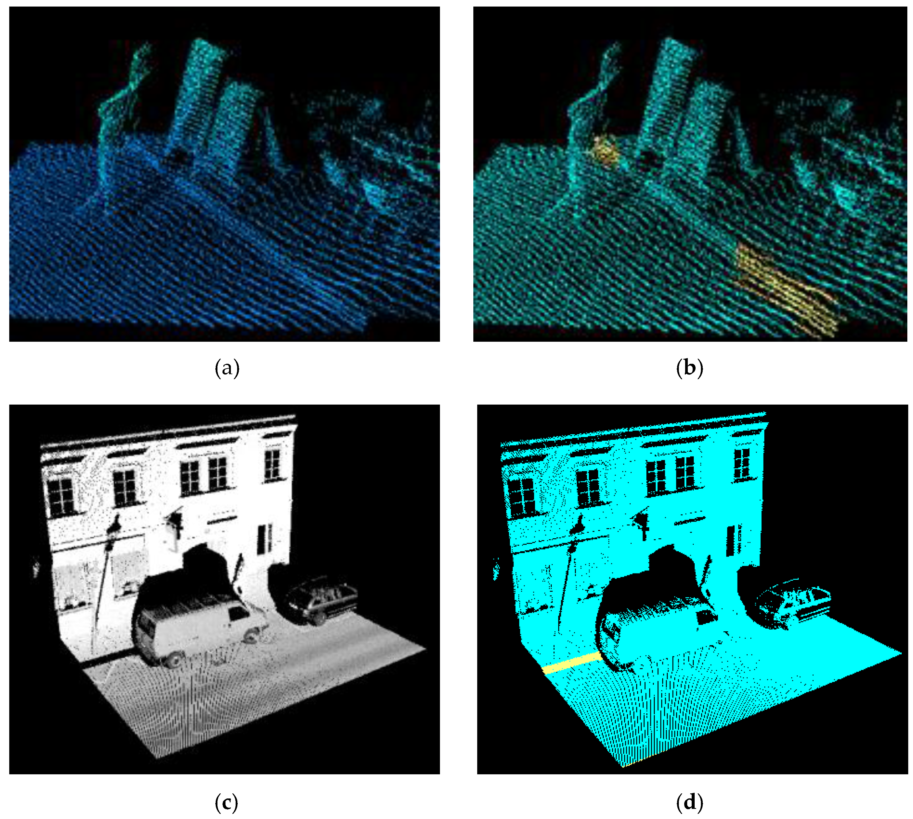
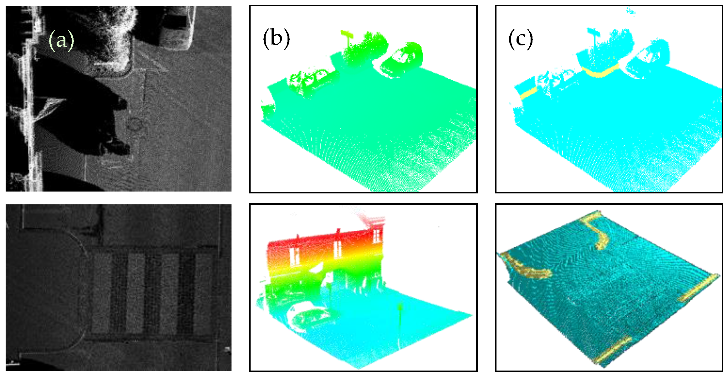
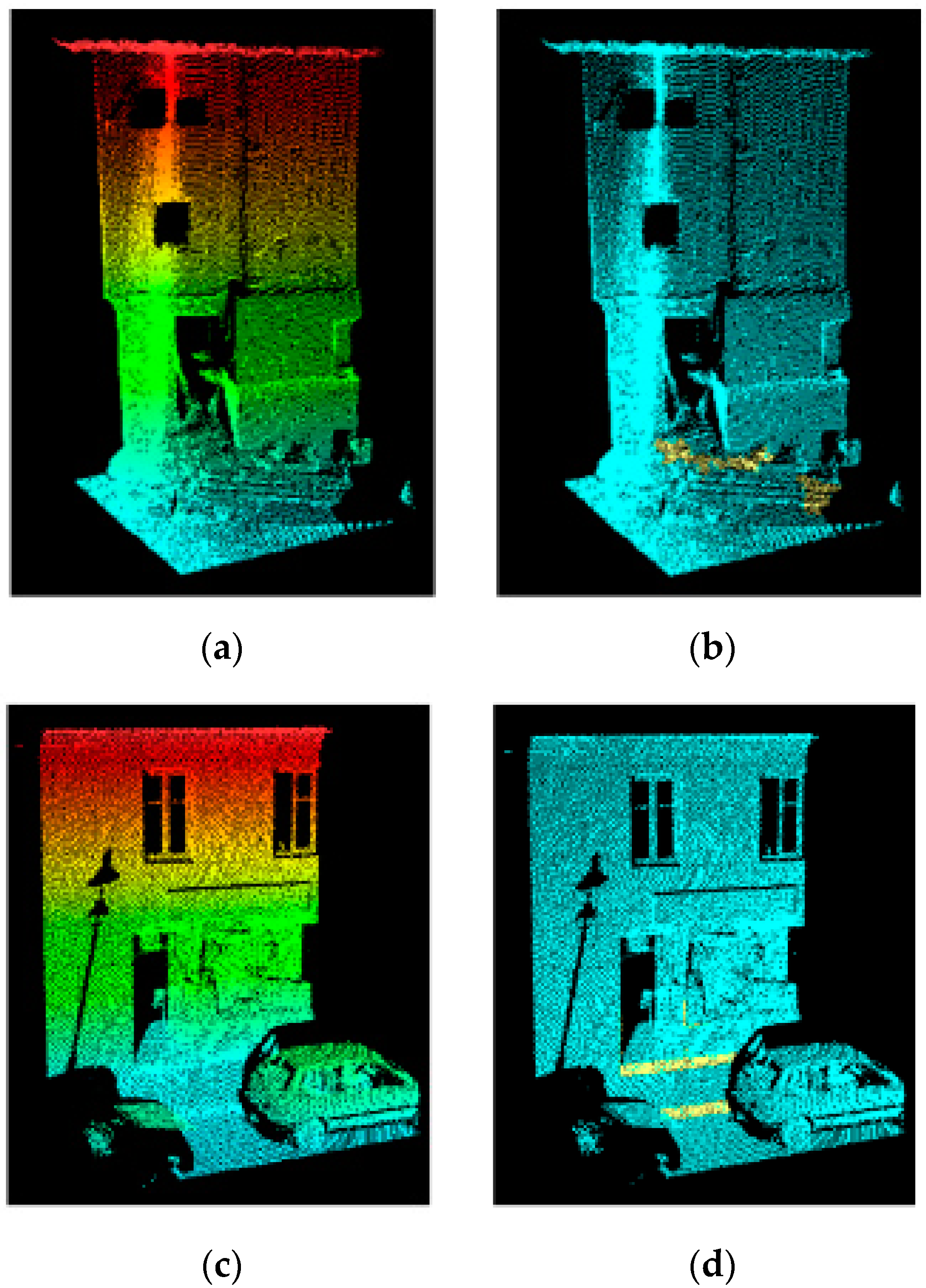
4. Results and Discussion
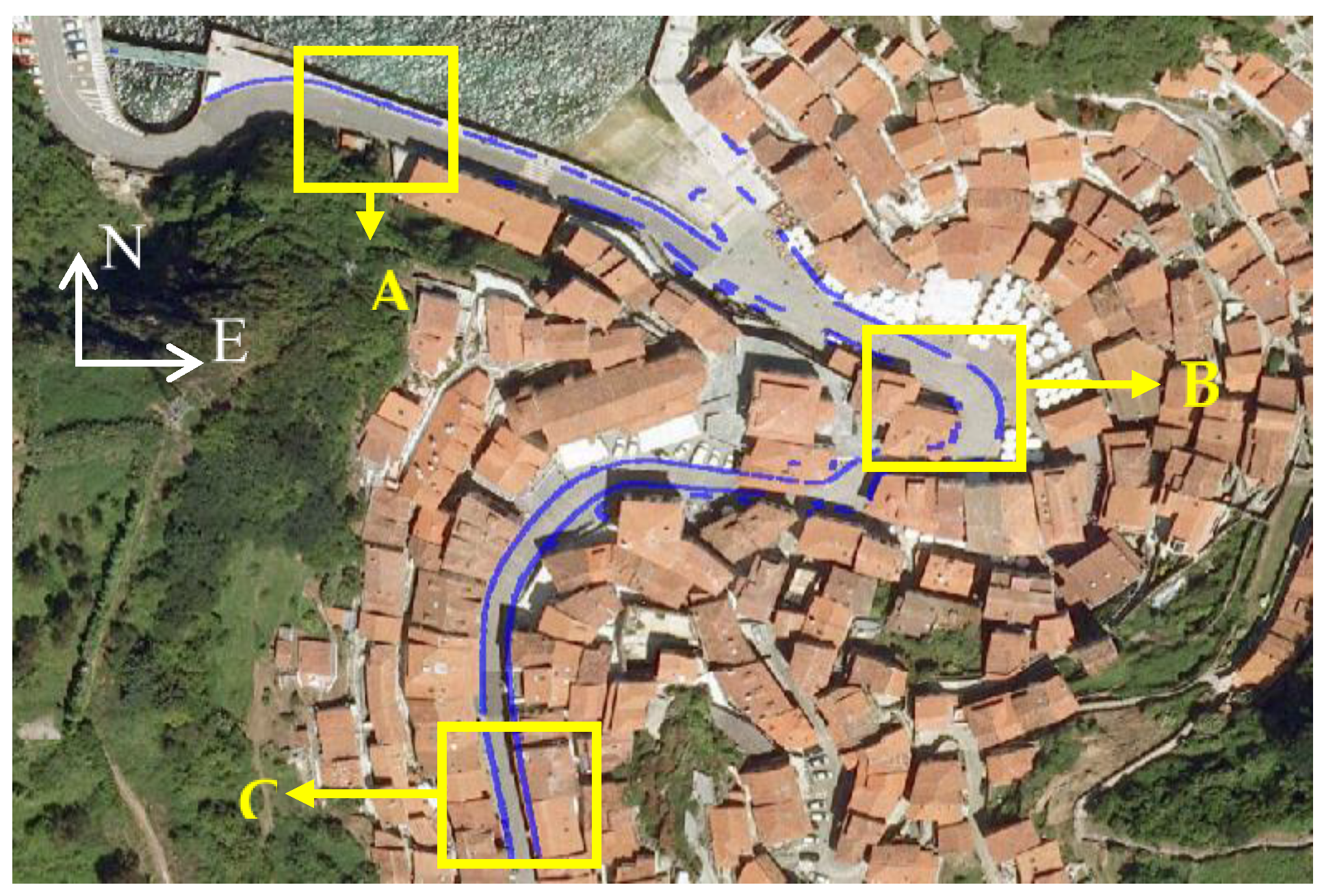
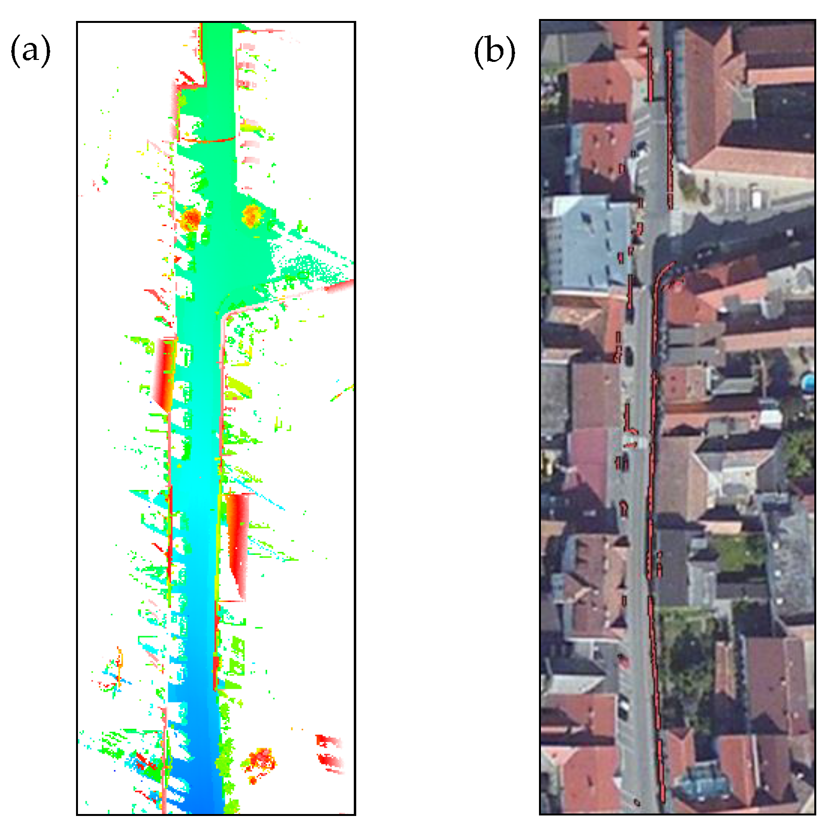
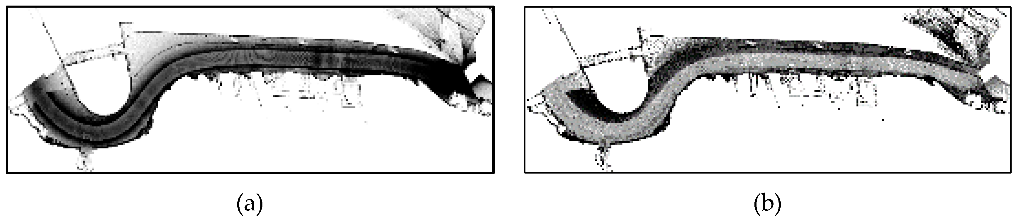
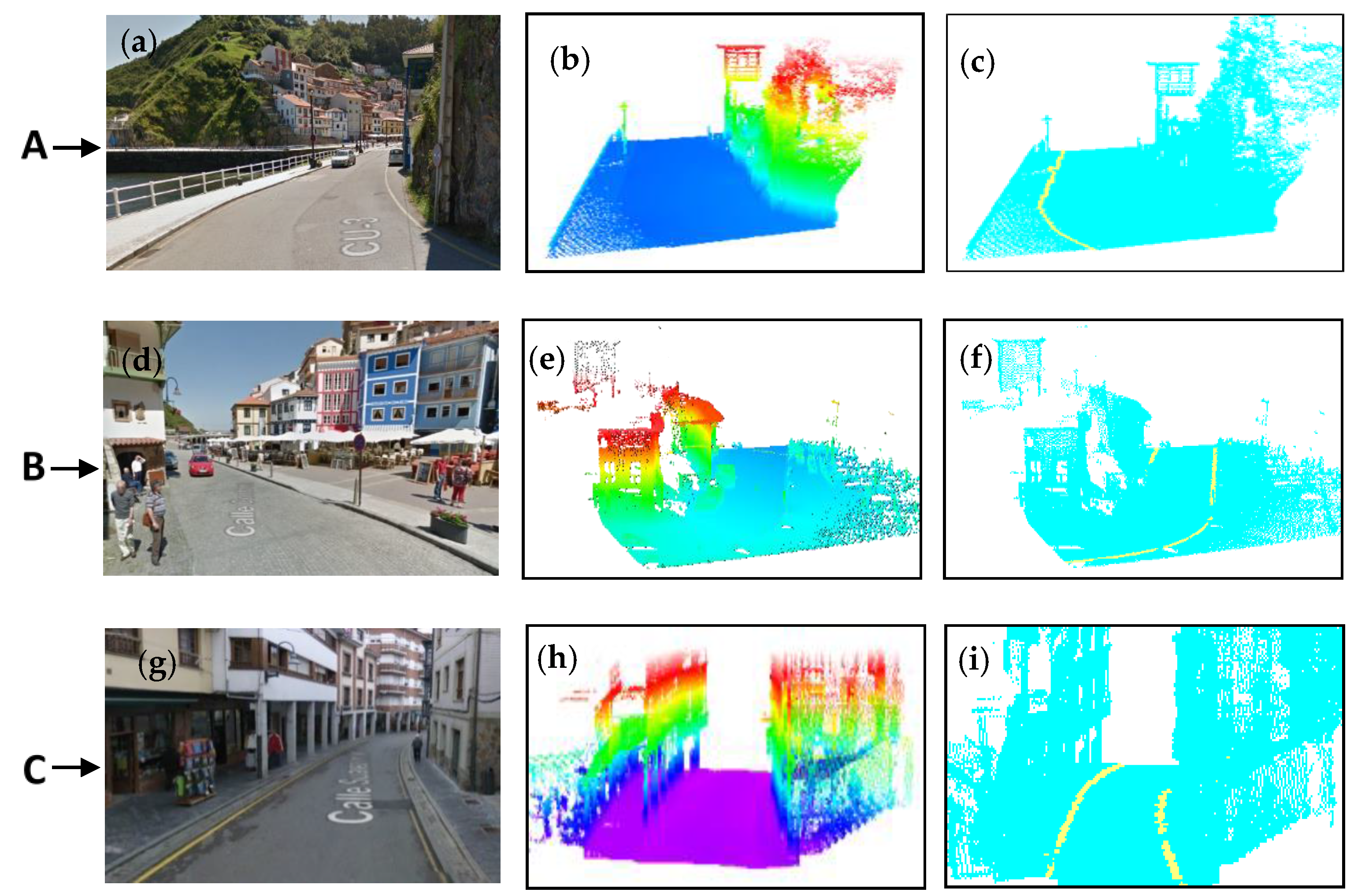
4.1. Test Site 1: Curb Representation and Accuracy Evaluation
4.2. Test Site 2: Curb Representation and Accuracy Evaluation
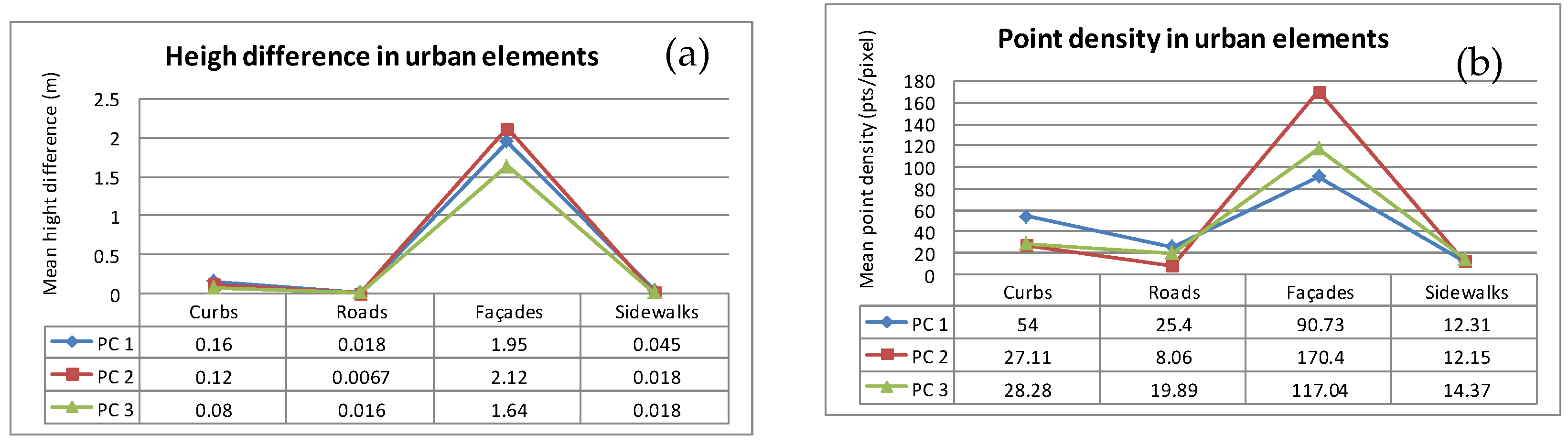
4.3. Parameters’ Sensibility Analysis
5. Conclusions
Acknowledgments
Author Contributions
Conflicts of Interest
References
- Wack, R.; Wimmer, A. Digital terrain models from airborne laserscanner data-a grid based approach. Int. Arch. Photogramm. Remote Sens. Spat. Inf. Sci. 2002, 34, 293–296. [Google Scholar]
- Rebecca, O.; Gold, C.; Kidner, D. 3d city modelling from LiDAR data. In Advances in 3d Geoinformation Systems; Springer: Berlin, Germany, 2008; pp. 161–175. [Google Scholar]
- Priestnall, G.; Jaafar, J.; Duncan, A. Extracting urban features from LiDAR digital surface models. Comput. Environ. Urban Syst. 2000, 24, 65–78. [Google Scholar] [CrossRef]
- Schmidt, R.; Weisser, H.; Schulenberg, P.; Goellinger, H. Autonomous driving on vehicle test tracks: Overview, implementation and results. In Proceedings of the IEEE Intelligent Vehicles Symposium, Dearborn, MI, USA, 3–5 October 2000; pp. 152–155.
- Urmson, C.; Anhalt, J.; Bagnell, D.; Baker, C.; Bittner, R.; Clark, M.; Dolan, J.; Duggins, D.; Galatali, T.; Geyer, C. Autonomous driving in urban environments: Boss and the urban challenge. J. Field Robot. 2008, 25, 425–466. [Google Scholar] [CrossRef]
- Ding, X.; Kang, W.; Cui, J.; Ao, L. Automatic extraction of road network from aerial images. In Proceedings of the 1st International Symposium on Systems and Control in Aerospace and Astronautics, Harbin, China, 19–21 January 2006.
- Cheng, X.-J.; Zhang, H.-F.; Xie, R. Study on 3d laser scanning modeling method for large-scale history building. In Proceedings of the International Conference on Computer Application and System Modeling (ICCASM), Taiyuan, China, 22–24 October 2010; pp. V7-573–V7-577.
- Gonzalez-Aguilera, D.; Muoz, A.; Lahoz, J.; Herrero, J.; Corchón, M.; Garcia, E. Recording and modeling paleolithic caves through laser scanning. In Proceedings of the International Conference on Advanced Geographic Information Systems &, Web Services, Cancun, Mexico, 1–7 February 2009; pp. 19–26.
- Argüelles-Fraga, R.; Ordóñez, C.; García-Cortés, S.; Roca-Pardiñas, J. Measurement planning for circular cross-section tunnels using terrestrial laser scanning. Autom. Constr. 2013, 31, 1–9. [Google Scholar] [CrossRef]
- Cabo, C.; Ordoñez, C.; García-Cortés, S.; Martínez, J. An algorithm for automatic detection of pole-like street furniture objects from mobile laser scanner point clouds. ISPRS J. Photogramm. Remote Sens. 2014, 87, 47–56. [Google Scholar] [CrossRef]
- Park, H.; Lim, S.; Trinder, J.; Turner, R. 3d surface reconstruction of terrestrial laser scanner data for forestry. In Proceedings of the IEEE International Geoscience and Remote Sensing Symposium (IGARSS), Honolulu, HI, USA, 25–30 July 2010; pp. 4366–4369.
- Rutzinger, M.; Elberink, S.O.; Pu, S.; Vosselman, G. Automatic extraction of vertical walls from mobile and airborne laser scanning data. Int. Arch. Photogramm. Remote Sens. Spat. Inf. Sci. 2009, 38, W8. [Google Scholar]
- Rutzinger, M.; Höfle, B.; Oude Elberink, S.; Vosselman, G. Feasibility of facade footprint extraction from mobile laser scanning data. Photogramm. Fernerkund. Geoinform. 2011, 2011, 97–107. [Google Scholar] [CrossRef]
- Hammoudi, K.; Dornaika, F.; Paparoditis, N. Extracting building footprints from 3d point clouds using terrestrial laser scanning at street level. ISPRS/CMRT09 2009, 38, 65–70. [Google Scholar]
- Yongtao, Y.; Li, J.; Haiyan, G.; Cheng, W.; Jun, Y. Semiautomated extraction of street light poles from mobile LiDAR point-clouds. IEEE Trans. Geosci. Remote Sens. 2015, 53, 1374–1386. [Google Scholar]
- Rodríguez-Cuenca, B.; García-Cortés, S.; Ordóñez, C.; Alonso, M.C. Automatic detection and classification of pole-like objects in urban point cloud data using an anomaly detection algorithm. Remote Sens. 2015, 7, 12680–12703. [Google Scholar] [CrossRef]
- Douillard, B.; Underwood, J.; Vlaskine, V.; Quadros, A.; Singh, S. A pipeline for the segmentation and classification of 3d point clouds. In Experimental Robotics; Springer: Berlin, Germany, 2014; pp. 585–600. [Google Scholar]
- Ioannou, Y.; Taati, B.; Harrap, R.; Greenspan, M. Difference of normals as a multi-scale operator in unorganized point clouds. In Proceedings of the 2012 Second International Conference on 3D Imaging, Modeling, Processing, Visualization and Transmission (3DIMPVT), Zurich, Switzerland, 13–15 October 2012; pp. 501–508.
- Yang, B.; Fang, L.; Li, J. Semi-automated extraction and delineation of 3d roads of street scene from mobile laser scanning point clouds. ISPRS J. Photogramm. Remote Sens. 2013, 79, 80–93. [Google Scholar] [CrossRef]
- Hu, H.; Munoz, D.; Bagnell, J.A.; Hebert, M. Efficient 3-d scene analysis from streaming data. In Proceedings of the 2013 IEEE International Conference on Robotics and Automation (ICRA), Karlsruhe, Germany, 6–10 May 2013; pp. 2297–2304.
- Ruyi, J.; Reinhard, K.; Tobi, V.; Shigang, W. Lane detection and tracking using a new lane model and distance transform. Mach. Vis. Appl. 2011, 22, 721–737. [Google Scholar] [CrossRef]
- Labayrade, R.; Douret, J.; Aubert, D. A multi-model lane detector that handles road singularities. In Proceedings of the 2006 IEEE Intelligent Transportation Systems Conference, Toronto, ON, Canada, 17–20 September 2006; pp. 1143–1148.
- Zhao, G.; Yuan, J. Curb detection and tracking using 3d-LiDAR scanner. In Proceedings of the 19th IEEE International Conference on Image Processing (ICIP), Orlando, FL, USA, 30 September–3 October 2012; pp. 437–440.
- Weiss, T.; Dietmayer, K. Automatic detection of traffic infrastructure objects for the rapid generation of detailed digital maps using laser scanners. In Proceedings of the IEEE Intelligent Vehicles Symposium, Istanbul, Turkey, 13–15 June 2007; pp. 1271–1277.
- Belton, D.; Bae, K.-H. Automating post-processing of terrestrial laser scanning point clouds for road feature surveys. Int. Arch. Photogramm. Remote Sens. Spat. Inf. Sci. 2010, 38, 74–79. [Google Scholar]
- Hervieu, A.; Soheilian, B. Semi-automatic road/pavement modeling using mobile laser scanning. City ISPRS Ann. Photogramm. Remote Sens. Spat. Inf. Sci. 2013, 2. [Google Scholar] [CrossRef]
- Kumar, P.; McElhinney, C.P.; Lewis, P.; McCarthy, T. An automated algorithm for extracting road edges from terrestrial mobile LiDAR data. ISPRS J. Photogramm. Remote Sens. 2013, 85, 44–55. [Google Scholar] [CrossRef]
- Serna, A.; Marcotegui, B. Urban accessibility diagnosis from mobile laser scanning data. ISPRS J. Photogramm. Remote Sens. 2013, 84, 23–32. [Google Scholar] [CrossRef]
- Trident Trimble Software. Available online: http://kmcgeo.com/Products/Trident/Trident_Feature_Table.pdf (accessed on 5 March 2016).
- Lehtomäki, M.; Jaakkola, A.; Hyyppä, J.; Kukko, A.; Kaartinen, H. Detection of vertical pole-like objects in a road environment using vehicle-based laser scanning data. Remote Sens. 2010, 2, 641–664. [Google Scholar] [CrossRef]
- Gonzalez, R.C.; Woods, R.E. Digital Image Processing; Prentice Hall: Englewood Cliff, NJ, USA, 2002. [Google Scholar]
- Cloudcompare Wiki Main Page. Available online: http://www.cloudcompare.org/doc/wiki/index.php?title=Main_Page (accessed on 17 December 2015).
- Mongus, D.; Lukač, N.; Žalik, B. Ground and building extraction from LiDAR data based on differential morphological profiles and locally fitted surfaces. ISPRS J. Photogramm. Remote Sens. 2014, 93, 145–156. [Google Scholar] [CrossRef]
- Heipke, C.; Mayer, H.; Wiedemann, C.; Jamet, O. Evaluation of automatic road extraction. Int. Arch. Photogramm. Remote Sens. 1997, 32, 151–160. [Google Scholar]
- Hu, J.; Razdan, A.; Femiani, J.C.; Cui, M.; Wonka, P. Road network extraction and intersection detection from aerial images by tracking road footprints. IEEE Trans. Geosci. Remote Sens. 2007, 45, 4144–4157. [Google Scholar] [CrossRef]


| Algorithm Settings | |
|---|---|
| Pixel size | 20 cm × 20 cm |
| Δh (Hmin and Hmax) | 0.05 < nDSM < 0.20 |
| Minimum point density (Dmin) | 20 points/pixel |
| Roughness (Redges) | 2.5 |
| Roughness neighborhood | 12 cm |
| Test Site 1 | Data Present Curbs |
|---|---|
| Algorithm detected (AD) | 525.1 m |
| User detected (UD) | 519.5 m |
| False positive (FP) | 35.8 m |
| False negative (FN) | 30.2 m |
| True positive (TP = AD − FP) | 489.3 m |
| Evaluation indices | |
| Completeness | 94.2% |
| Correctness | 93.2% |
| Quality | 88.11% |
| Pixel Size | 5 cm × 5 cm |
|---|---|
| Δh (Hmin and Hmax) | 0.1 < nDSM < 0.20 |
| Point density (Dmin) | 20 points/pixel |
| Roughness (Redges) | 2.5 |
| Roughness neighborhood | 12 cm |
| Test Site 2 | Data Present Curbs |
|---|---|
| Algorithm detected (AD) | 231.61 m |
| User detected (UD) | 224.76 m |
| False positive (FP) | 21.4 m |
| False negative (FN) | 14.55 m |
| True positive (TP = AD − FP) | 210.21 m |
| Evaluation indices | |
| Completeness | 93.52% |
| Correctness | 90.76% |
| Quality | 85.42% |
| Considered Parameters | Parameter Ranges |
|---|---|
| Pixel size | 4–5 times the distance between consecutive scans |
| Δh (Hmin and Hmax) | [0.05; 0.10] m < nDSM < [0.15; 0.20] m |
| Minimum point density (Dmin) | [15; 25] points/pixel |
| Roughness (Redges) | [2; 2.5] roughness |
| Roughness neighborhood | [10; 20] cm |
| Considered Parameters | Completeness | Correctness | Quality |
|---|---|---|---|
| Pixel size 1 time distance between consecutive scans | 67.3% | 97.2% | 66.03% |
| Pixel size 5 times distance | 94.2% | 93.2% | 88.1% |
| Pixel size 10 times distance | 93.3% | 88.3% | 83.1% |
| Δh (Hmin and Hmax) = [0.02; 0.17] m | 98.1% | 71.8% | 70.8% |
| Δh = [0.07; 0.17] m | 94.2% | 93.2% | 88.1% |
| Δh = [0.07; 0.35] m | 97.1% | 74.3% | 72.7% |
| Minimum point density (Dmin) = 5 | 42.3% | 95.7% | 41.5% |
| Minimum point density (Dmin) = 20 | 94.2% | 93.2% | 88.1% |
| Minimum point density (Dmin) = 50 | 98.1 | 77.3% | 76.11% |
© 2016 by the authors; licensee MDPI, Basel, Switzerland. This article is an open access article distributed under the terms and conditions of the Creative Commons Attribution (CC-BY) license (http://creativecommons.org/licenses/by/4.0/).
Share and Cite
Rodríguez-Cuenca, B.; García-Cortés, S.; Ordóñez, C.; Alonso, M.C. Morphological Operations to Extract Urban Curbs in 3D MLS Point Clouds. ISPRS Int. J. Geo-Inf. 2016, 5, 93. https://doi.org/10.3390/ijgi5060093
Rodríguez-Cuenca B, García-Cortés S, Ordóñez C, Alonso MC. Morphological Operations to Extract Urban Curbs in 3D MLS Point Clouds. ISPRS International Journal of Geo-Information. 2016; 5(6):93. https://doi.org/10.3390/ijgi5060093
Chicago/Turabian StyleRodríguez-Cuenca, Borja, Silverio García-Cortés, Celestino Ordóñez, and María C. Alonso. 2016. "Morphological Operations to Extract Urban Curbs in 3D MLS Point Clouds" ISPRS International Journal of Geo-Information 5, no. 6: 93. https://doi.org/10.3390/ijgi5060093
APA StyleRodríguez-Cuenca, B., García-Cortés, S., Ordóñez, C., & Alonso, M. C. (2016). Morphological Operations to Extract Urban Curbs in 3D MLS Point Clouds. ISPRS International Journal of Geo-Information, 5(6), 93. https://doi.org/10.3390/ijgi5060093