Abstract
The availability of nighttime satellite imagery provides unique opportunities for monitoring fishing activity in data-sparse ocean regions. This study leverages Visible Infrared Imaging Radiometer Suite (VIIRS) Day/Night Band monthly composite imagery to identify and classify recurring spatial patterns of fishing activity in the Korean Exclusive Economic Zone from 2014 to 2024. While prior research has primarily produced static hotspot maps, our approach advances geospatial fishing activity identification by employing machine learning techniques to group similar spatiotemporal configurations, thereby capturing recurring fishing patterns and their temporal variability. A convolutional autoencoder and a Gaussian Mixture Model (GMM) were used to cluster the VIIRS imagery. Results revealed seven major nighttime light hotspots. Results also identified four cluster patterns: Cluster 0 dominated in December, January, and February, Cluster 1 in March, April, and May, Cluster 2 in July, August, and September, and Cluster 3 in October and November. Interannual variability was also identified. In particular, Clusters 0 and 3 expanded into later months in recent years (2022–2024), whereas Cluster 1 contracted. These findings align with environmental changes in the region, including ocean temperature rise and declining primary productivity. By integrating autoencoders with probabilistic clustering, this research demonstrates a framework for uncovering recurrent fishing activity patterns and highlights the utility of satellite imagery with GeoAI in advancing marine fisheries monitoring.
1. Introduction
The use of satellite imagery has proven to be very effective in detecting fishing activities [1]. Among the various data sources available, nighttime light imagery, particularly from the Visible Infrared Imaging Radiometer Suite (VIIRS) Day/Night Band (DNB), has emerged as a valuable resource for identifying and tracking fishing activities in ocean areas that are otherwise difficult to access and monitor [2,3]. The nighttime imagery is especially crucial for observing light-luring fisheries and serves as an important complement to other monitoring systems like the Automatic Identification System (AIS) [4]. The ability of VIIRS to provide a consistent, long-term record of fishing-related light emissions offers a unique and powerful way to track changes in human activity at sea over vast temporal and spatial scales.
Many studies have used VIIRS nighttime imagery to identify fishing hotspots, utilizing the brightness of lights at sea as proxies for fishing vessel activity [5,6,7,8]. Such efforts have significantly advanced our ability to detect and monitor fishing activities at sea. However, despite the wealth of data and the clear spatial patterns emerging from satellite observations, little attention has been given to clustering recurring patterns to identify typical geographical configurations of fishing activity. Previous work has largely focused on producing monthly or annual hotspot maps (e.g., [2,7,8,9,10,11,12,13]). This study takes a step further by clustering similar monthly patterns into shared categories. This new approach may make it possible to characterize typical spatial configurations of fishing activity and to evaluate whether particular months conform to or diverge from these recurring patterns potentially in connection with global environmental changes such as global warming. In this endeavor, recent progress in machine learning methods like autoencoders [3,14,15,16] and clustering techniques [17,18,19] may help extract latent representations from high-dimensional spatial data and uncover structures not readily apparent through conventional mapping or descriptive analysis. To date, no study has systematically applied such methods to classify spatial fishing behaviors or develop typologies of recurring activity, leaving a gap in understanding where fleets operate consistently over time.
To address the gap, this research presents a machine learning framework for identifying and characterizing distinctive fishing area patterns within the Korean Exclusive Economic Zone (EEZ). The primary objectives are threefold: first, to map light intensities to identify where most nighttime fishing activities occur; second, to identify unique spatial patterns of fishing locations from VIIRS DNB monthly composite images; and third, to investigate how these patterns are associated with different calendar months or years. The methodological approach involves using a deep learning-based autoencoder to extract robust, non-linear features from the imagery, followed by a probabilistic Gaussian Mixture Model (GMM) to cluster the data into meaningful patterns.
The remainder of this paper is organized as follows. Section 2 describes the study area, datasets, and methodological framework, including the architecture and training of the convolutional autoencoder and the subsequent clustering analysis using the Gaussian Mixture Model. Section 3 presents the results, focusing on the identified spatial clusters and their monthly and interannual variations. Section 4 discusses the implications of these findings for fisheries monitoring and management, as well as methodological considerations for future research. Finally, Section 5 concludes with a summary of key findings and their significance for GeoAI–based fisheries assessment and marine resource management.
2. Methodology
2.1. Study Area
The Exclusive Economic Zone of the Republic of Korea (Republic of Korea) [20] covers parts of the Yellow Sea, the East China Sea, and the East Sea (Sea of Japan). Figure 1 shows the EEZ, buffered 10 km from coastlines, together with warm and cold currents and the Provisional Measure Zones (PMZs). PMZs represent joint fishing areas established between South Korea and neighboring countries. One PMZ in the Yellow Sea is shared with China, while the PMZs in the East China Sea and the East Sea are jointly shared with Japan. The Yellow Sea is shallow (less than 80 m deep) with wide continental shelves, while the East Sea has deep basins that exceed 2000 m [21]. The EEZ is influenced by several ocean current systems. The Kuroshio Current extends into the East China Sea, the Tsushima Warm Current enters the East Sea, and the North Korea Cold Current flows southward along the east coast [21]. The interaction of these currents produces seasonal fronts and stratification. Hydrographic conditions change with season and affect primary productivity. The total area of the Korean EEZ is about 349,609 km2.
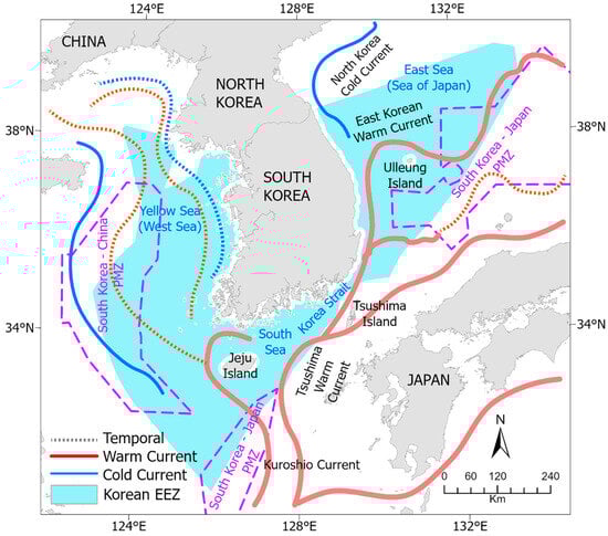
Figure 1.
Study area. PMZ denotes a joint fishing area between countries with overlapping boundaries of interest, such as EEZs. The Korean EEZ was buffered 10 km from the coastline.
According to Korea’s National Institute of Fisheries Science [22], sea surface temperatures around the Korean Peninsula have increased by 1.58 °C over the period 1968–2024, a rate more than twice the global average of 0.74 °C. The East Sea recorded the most pronounced warming, with a temperature rise of 2.04 °C, followed by Yellow Sea of 1.44 °C and South Sea of 1.27 °C. Along with these thermal changes, Chlorophyll-a concentrations—used as a proxy for phytoplankton biomass and primary productivity—have shown a declining trend since 2003, particularly in the central sectors of the Yellow Sea and East Sea. In 2024, primary productivity declined by 21.6% compared to the previous year, reflecting a significant reduction in the ocean’s biological capacity. Aquaculture losses in 2024 amounted to KRW 143 billion, the highest annual figure since 2012. Coastal and nearshore fishery production has also decreased substantially, from 1.51 million tons in the 1980s to approximately 0.84 million tons in 2024 [22]. These changes are attributed to enhanced Tsushima Warm Current activity and broader climatic shifts, including the weakening of the East Asian Winter Monsoon [23].
The Korean EEZ supports diverse fisheries. Major species include anchovy (Engraulis japonicus), chub mackerel (Scomber japonicus), yellow croaker (Larimichthys polyactis), cod (Gadus macrocephalus), flatfish, and others [21,22,24]. Several fisheries employ night-fishing lights. Japanese flying squid (Todarodes pacificus) is targeted mainly in the East Sea from late spring to autumn. Hairtail (Trichiurus lepturus), Pacific saury (Cololabis saira), anchovy, blue crab, and mackerel are also taken with light attraction. The use of high-intensity lights makes these vessels visible to satellite nighttime sensors. Fishing activity in the EEZ shows seasonal and spatial variation according to oceanographic conditions and species distribution [25]. These conditions make the area suitable for analyzing spatiotemporal patterns of vessel lights using satellite data.
2.2. Data
The VIIRS sensor, launched in 2011, collects imagery across 22 spectral bands that are composed of 16 moderate-resolution bands (M-bands), five imaging-resolution bands (I-bands), and one panchromatic Day/Night Band [26]. The DNB has a 742 m spatial resolution across a swath of approximately 3000 km and is centered at a wavelength of 0.7 μm (i.e., 0.5 μm–0.9 μm wavelength range). While originally developed to provide continuous cloud imagery, the DNB has become widely used for nighttime light studies thanks to its ability to capture low-light conditions on a global scale [27]. Since 2015, the Earth Observation Group (EOG) has produced global VIIRS Nighttime Lights (VNL) monthly composite products. These composites are generated by filtering sunlit and moonlit, stray light, lightning, cloud, and transient outliers such as biomass burning, aurora, and high-energy particle events [28,29]. Pixel values in each VIIRS composite image represent top-of-atmosphere radiance (nW·cm−2·sr−1).
This study used VNL monthly composite data from January 2014 to December 2024. A total of 132 images were obtained from Google Earth Engine, clipped to the Korean EEZ boundary shapefile that was downloaded from https://marineregions.org (accessed on 27 September 2025) [30]. All images were reprojected to EPSG:5179 (KGD2002/Unified CS). Pixel values greater than 15,000 or less than zero were excluded, and areas within 10 km of the EEZ boundary were masked to minimize lights from land. Finally, pixel values were aggregated to a 10 km grid (104 × 104 pixels) using mean resampling.
2.3. Analytical Framework
2.3.1. Convolutional Autoencoder
A convolutional autoencoder (CAE) framework (Figure 2) was implemented to identify spatiotemporal similarity patterns among monthly VIIRS DNB composite images. In contrast to convolutional neural network (CNN) methods that are primarily used for object detection and classification in images [31], the convolutional autoencoder is an unsupervised learning model designed to discover underlying patterns in images through multilevel feature extraction. The CAE is a variant of the autoencoder that employs convolutional layers, which makes it more suitable for processing 2D data with spatial patterns compared with conventional autoencoders [32,33]. Recently, CAE has been applied to various satellite imagery and time-series image analysis tasks, leveraging spatiotemporal features to compress high-dimensional image data into informative latent representations [34,35].
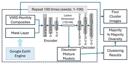
Figure 2.
Workflow of analyses with the convolutional autoencoder–Gaussian Mixture Model (CAE–GMM).
Because the 10 km grid dimension (104 × 104 pixels) is divisible by eight, no additional padding operation was required. Pixels explicitly coded as –1 were treated as NoData throughout training and evaluation, ensuring that missing or masked regions did not bias latent feature extraction. The binary mask channel assigned a value of 1 to valid ocean pixels and 0 to masked land or NoData pixels. We tested both individual and global normalization; individual normalization with valid pixels was selected for the final analysis as it better preserved the relative spatial patterns within each month, which was the primary focus of our clustering. Each normalized image was concatenated with a binary mask channel, resulting in a two-channel input (i.e., radiance and mask). The autoencoder architecture followed a balanced encoder–decoder structure with filter depths of 16, 32, and 64, and a latent dimensionality of 64. The encoder consisted of three convolutional blocks using a 3 × 3 kernel and the Rectified Linear Unit (ReLU) activation function, with stride-2 downsampling and batch normalization, followed by a fully connected latent layer with L2 regularization. This specific configuration was chosen based on empirical tuning with multiple hyperparameter combinations in order to balance model performance with the limited dataset size (n = 132), ensuring robust feature extraction while mitigating the risk of overfitting. The decoder mirrored this structure using transposed convolutions to reconstruct the input radiance patterns. The final output layer employed a 3 × 3 convolution with a linear activation function to accurately predict continuous normalized pixel intensities. The mean squared error (MSE) was used as loss function. This loss calculation was performed exclusively over valid pixels by applying the binary mask channel, ensuring that land or boundary artifacts did not bias the result.
Training was performed using the Adam optimizer (learning rate = 1 × 10⁻⁴), a batch size of 8, and a maximum of 300 epochs. Early stopping with a patience of 20 epochs was applied to prevent overfitting. The model’s reproducibility was ensured by fixing random seeds for Python 3.11.13, NumPy 2.0.2, and TensorFlow 2.18.1. After optimization, the encoder was used to extract 64-dimensional latent feature vectors for each image, representing compressed spatial–radiometric structures of nocturnal fishing activities within the Korean EEZ.
2.3.2. Gaussian Mixture Model
The latent feature vectors were standardized using z-score normalization, calculated across all 132 samples, and then used for unsupervised clustering. A Gaussian Mixture Model (GMM) [36] was adopted since it allows full covariance to represent anisotropic (elliptical) clusters, provides soft assignments that quantify uncertainty in ambiguous boundary regions, and offers likelihood-based criteria for model selection. Compared with hard-partitioning methods like k-means clustering, GMM is therefore better suited for handling the elongated and overlapping spatial patterns [18,37,38,39,40].
The optimal number of clusters (k) was determined by minimizing the Bayesian Information Criterion (BIC) across k values from 2 to 10. To assess robustness, the CAE–GMM was executed 100 times using different random seeds (1–100). For each run, cluster stability was also evaluated by running the GMM 10 times with different initializations and computing pairwise Adjusted Rand Index (ARI) and Normalized Mutual Information (NMI) values. Also, cluster centroids in the latent space were decoded using the trained decoder to generate representative images for k clusters.
The multiple GMM clustering outputs were post-processed using the Hungarian algorithm [41] to align cluster IDs across different runs, since the unsupervised GMM clustering assigns cluster labels arbitrarily. Subsequently, the mode cluster values across the multiple iterations were selected to determine the most frequently occurring cluster pattern for each month and year. This ensemble-based approach enhances the stability and robustness of the clustering results, avoiding dependence on a single random initialization. Furthermore, the percentage occurrence of each mode value over the 11-year period was calculated to quantify the temporal variability and stability of monthly cluster patterns. Finally, mean radiance composites were generated for each mode-value cluster, serving as representative images of their spatial radiance patterns.
3. Results
3.1. Intensity of Nighttime Lights
The intensities of nighttime lights were obtained by calculating mean values from the original 132 monthly composite images in the 500 m grid. The resulting map (Figure 3) illustrates the spatial distribution of nighttime lights observed by VIIRS DNB. The highest concentrations of nightlight activity are distinctly visible around Jeju Island, extending eastward through the Korea Strait, suggesting sustained and concentrated fishing operations in these southern coastal waters. Intense light emissions are also evident in the South Korea–China PMZ in the Yellow Sea and the South Korea–Japan PMZ in the East China Sea. A northward linear patch also appears in the Yellow Sea between the Korean Peninsula and the South Korea–China PMZ. Along the eastern coast of the Korean Peninsula, nightlight intensities appear more dispersed, extending offshore toward the west-side of Ulleung Island. Patches also appear around Ulleung and Dokdo Islands, and at the far northeastern corner of the Korean EEZ where the Yamato Rise provides optimal habitat for multiple fish species. In total, about seven hotspots are identified: (1) South Korea–China PMZ, (2) linear and northward stretch at the Yellow Sea, (3) around Jeju Island, (4) South Sea stretch from Jeju Island through the Korea Strait, (5) wide and linear northward stretch along the east coast of the Korean peninsula, (6) around the Ulleung and the Dokdo Islands, and (7) the northeast corner of the Korean EEZ. Overall, the light intensity map captures clear geographical hotspots and gradients in fishing intensity, strongest in the South Sea and tapering northward into the Yellow and East Seas.
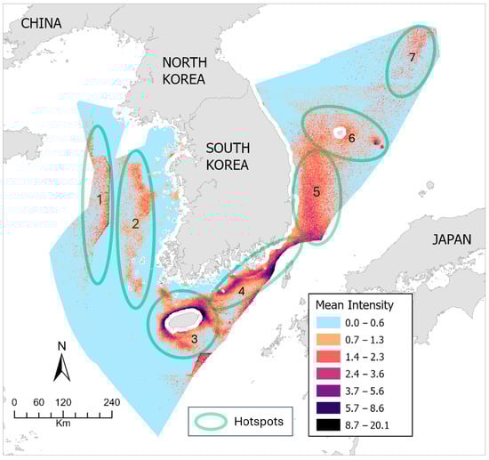
Figure 3.
Mean nighttime light intensity (2014–2024). The numbered labels represent provisionally assigned hotspot reference IDs.
3.2. Spatial Cluster Patterns
Out of the 100 clustering runs, GMM identified four clusters (k = 4) in 84 runs, while 16 runs produced five clusters (k = 5), suggesting that the monthly VIIRS composites are optimally represented by four distinct clusters. The mean Adjusted Rand Index and Normalized Mutual Information from the 84 runs with k = 4 were 0.412 (σ = 0.117) and 0.476 (σ = 0.098), respectively. These values indicate a moderate but consistent level of clustering stability and reproducibility, confirming that the CAE–GMM framework provides reliable and coherent partitioning of spatiotemporal nightlight patterns.
Figure 4 is an example of training loss trend, GMM BIC trend for k = [2–10], and ARI and NMI distributions with 10 runs, obtained with the seed value of 83. The example clearly reveals that loss function is converging well, k = 4 is the best, and the mean ARI (0.481) and NMI (0.528) are moderate though their median values are slightly lower than the means. Figure 4e–h also shows decoded cluster pattern images from the mean latent vectors extracted from 132 input images.
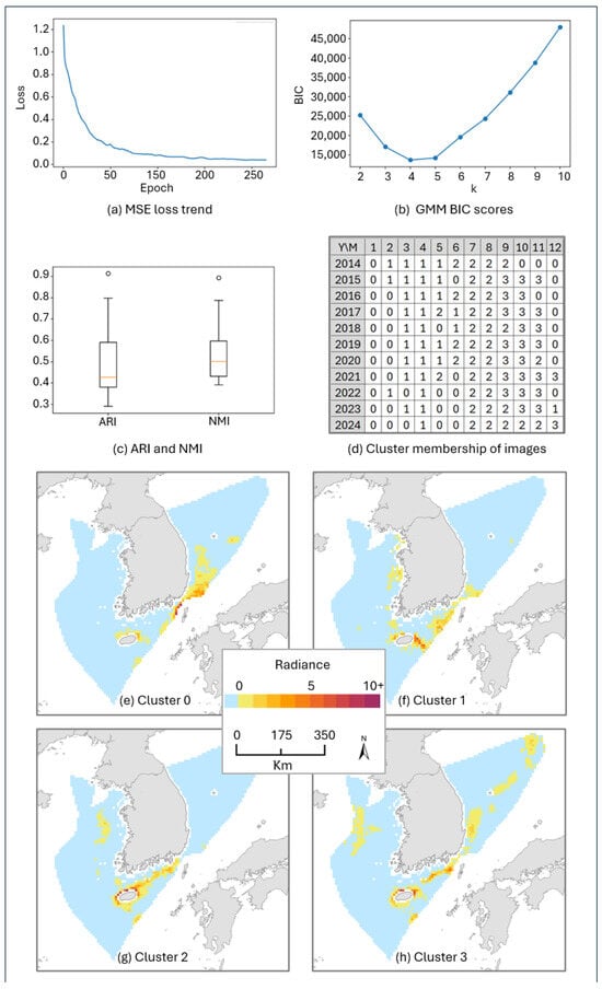
Figure 4.
An example of CAE-GMM outputs with the random seed value of 83. (a) Mean squared error (MSE) loss trend of the CAE. (b) BIC scores of the GMM for k = [2, 10]. (c) ARI and NMI distributions from 10 runs with k = 4. (d) Cluster membership table of the input images. (e–h) The decoded, imaginary images that were created with mean latent vectors. The legend for (e–h) indicates radiance (nW cm−2 sr−1).
Figure 5 illustrates the four representative cluster patterns (Clusters 0–3), each derived from the mean radiance composites corresponding to their respective mode-defined clusters. Cluster 1 exhibits the lowest nightlight intensity among the four (range = 0.16–6.96, mean = 0.35), with sparse fishing activities concentrated around Jeju Island and along the EEZ boundary with Japan in the South Sea. Cluster 2 presents a higher level of illumination (range = 0.19–17.43, mean = 0.74), primarily distributed from Jeju Island through the Korea Strait, indicating intensified fishing activity. Light patches also appear in both the Yellow Sea and East Sea, though their brightness remains lower compared to the Jeju–Korea Strait corridor. Interestingly, little lights appear at the South Korea–China PMZ, the joint fishing area between Korea and China, in the Yellow Sea. Cluster 3 represents the most extensive and intense nightlight pattern (range = 0.27–18.17, mean = 0.93). While the South Sea retains a pattern similar to Cluster 2, the spatial extent slightly contracts. In contrast, the East Sea exhibits widespread illumination stretching from Busan to Ulleung Island and reaching the northeastern corner of the Korean EEZ, while in the Yellow Sea, light activities concentrate at the South Korea–China PMZ. Finally, Cluster 0 (range = 0.18–15.07, mean = 0.64) shows weak and scattered light presence around Jeju Island and the Yellow Sea, yet a broad, continuous concentration appears along the Tsushima–Ulleung corridor. Quantitatively, Cluster 3 recorded the highest mean radiance, followed by Cluster 2 and Cluster 0, with Cluster 1 exhibiting the lowest intensity. This distinct minimum in Cluster 1 aligns with its temporal dominance in early spring, a period typically associated with reduced fishing effort.
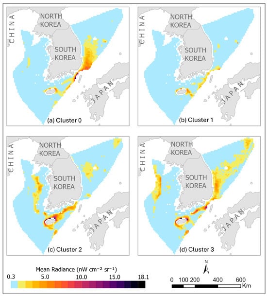
Figure 5.
Spatial patterns of the four clusters identified by the CAE–GMM framework. Each subfigure (a–d) represents the mean radiance of the images assigned to the corresponding cluster.
3.3. Temporal Cluster Patterns
To determine the predominant pattern for each month and year, the mode cluster values were calculated across the 84 clustering runs that produced k = 4 clusters. Table 1 summarizes the occurrence of the four spatial patterns based on these mode values. Among all runs, the clustering with the seed value 83 showed the highest agreement (91.7%) with the mode configuration.

Table 1.
Most frequent categories and their percentage occurrences across 84 CAE-GMM clustering attempts. Colors indicate four identified categories. Units: mode category and its percentage occurrence (in parentheses).
Table 1 reveals clear seasonal transitions and recent shifts in cluster distribution patterns. Cluster 0 is predominantly observed in January and February, reflecting its strong association with early winter conditions. Cluster 1 becomes dominant in March and April, extending into May during the earlier years, but its dominance in May has gradually been replaced by Cluster 0 since 2022, suggesting a seasonal advancement of Cluster 0 characteristics. June historically exhibits mixed occurrences of Clusters 1, 2, and 3, but has also been increasingly dominated by Cluster 0 in recent years. In contrast, Cluster 2 consistently dominates July and August, representing a stable and persistent summer pattern, while September remains mostly under Cluster 2 but shows temporary Cluster 3 influence between 2020 and 2022. October and November are largely governed by Cluster 3, corresponding to late-autumn conditions. Notably, December, which was once dominated by Cluster 0, has seen Clusters 1 and 3 emerging since 2019, implying more variable year-end conditions. Overall, the results depict a stable seasonal cycle—Cluster 0 (December–February), Cluster 1 (March–May), Cluster 2 (July–August), and Cluster 3 (October–November)—with recent expansions of Cluster 3 into December and Cluster 0 into late spring months, signaling evolving climatic or environmental transitions.
When the modal percentages were analyzed to assess the consistency and stability of cluster assignments, the months of January, July, August, and September exhibited relatively high values—suggesting these months tend to follow a consistent clustering pattern (Table 1). In contrast, May, June, November, and December displayed lower modal percentages, pointing to greater variability in their cluster designations. Additionally, a noticeable decline in pattern stability is observed in the years following 2020, with the exception of August, which maintained its consistency despite the broader trend.
When examining the number of unique cluster occurrences per cell (i.e., cluster diversity), January through March generally exhibited three distinct clusters, whereas April through June and October through November commonly displayed four. August typically showed the lowest diversity with only two clusters. In contrast, July and September, which initially exhibited two dominant clusters, have shown an increase to three or four clusters since 2020. December, which previously featured three clusters, has consistently shown four since 2019, indicating a rise in cluster variability. Overall, these results reveal a gradual increase in spatial–temporal diversity of fishing patterns after 2020, particularly in July, September, and December. When the proportions of the two most frequent clusters in each cell were calculated, they were generally above 80%, implying that most cells were characterized by at most two dominant spatial patterns interplayed. However, notable declines in these percentages were observed in May, June, and December during 2023 and 2024, suggesting heightened variability and instability in fishing activity during these periods.
4. Discussion
4.1. CAE–GMM Framework
This study demonstrates that combining a convolutional autoencoder with a Gaussian Mixture Model can effectively capture recurring spatiotemporal fishing patterns from VIIRS DNB imagery. The CAE learns a compact latent representation of high-dimensional satellite images by minimizing the reconstruction loss. In this work, the encoder compressed the radiance distribution of the Korean EEZ into a 64-dimensional latent space, effectively summarizing complex spatial features into a manageable numerical vector. To enhance robustness, 100 independent GMM clustering runs were executed with different seed numbers. The consistent identification of four clusters (in 84 of 100 runs) and moderate reproducibility (mean ARI = 0.412, NMI = 0.476) confirm that the CAE–GMM framework produces reliable yet flexible partitioning of fishing activity patterns. The presence of visually distinctive spatial patterns and temporal coherence further supports the validity of these outputs, demonstrating that the framework serves as a robust tool for the long-term monitoring of fishing area dynamics.
4.2. Seasonal and Regulatory Influences on Fishing Activity
The four clusters revealed by the CAE–GMM correspond closely to seasonal fisheries cycles and regulatory constraints in the Korean EEZ and PMZs. Specifically, Cluster 2 (summer) exhibits low activity in the South Korea–China PMZ, whereas Cluster 3 (autumn) shows intensified illumination in the same region. This shift aligns with China’s closed fishing season, which generally spans May–August. In South Korea, fishing vessel lights would also be affected by the fishing off-seasons. In 2024, for example, off-season species include Blue Crab (Portunus trituberculatus, 21 June–20 August), Japanese flying squid (Todarodes pacificus, 1 April–30 May), Spanish mackerel (Scomberomorus niphonius, 1 May–30 May), and mackerel (Scomber japonicus, one month in April–June). During these months, reduced activity in Cluster 2 likely reflects regulatory enforcement. The subsequent surge of activity in Cluster 3 (September–November) represents the resumption of fishing efforts following the closed seasons, highlighting the interplay between policy-driven temporal restrictions and observed satellite light patterns.
4.3. Contradiction Between Increased Light Coverage and Declining Fishery Tonnage
Despite the observed increase in light coverage—particularly the expansion of Cluster 0 and the emergence of Cluster 3 in December—official fisheries statistics indicate a decline in both total catch and fleet size since 2022 [22]. For instance, the annual production of major light-luring species, Todarodes pacificus (squid) and Trichiurus lepturus (hairtail), decreased by 71.6% and 22.6%, respectively, between 2021 and 2024 [42]. Over the same period, the gross tonnage of the jigging fleet with luring lights declined by approximately 18.1%, from 14,549 tons in 2021 to 11,917 tons in 2024 [43].
Within this context, the recent expansion of Cluster 0 and the appearance of Cluster 3 in December may reflect a redistribution of fishing effort rather than an increase in vessel numbers. One possible interpretation is that fishing vessels are operating over broader areas or adjusting their spatial search behavior in response to reduced resource availability. This interpretation is consistent with the prolonged low-resource conditions reported for 2017–2023 by Jo et al. [44], although direct causal links cannot be established in the present study. Nonetheless, the CAE–GMM framework provides a useful complementary perspective to conventional fisheries statistics by revealing spatiotemporal adjustments in fishing activity patterns, thereby helping to contextualize satellite-derived nightlight observations under changing environmental and economic conditions.
4.4. Influence of Environmental Factors
The temporal evolution of the clusters also appears to reflect reported environmental trends. For example, sea surface temperatures around the Korean Peninsula have risen by 1.58 °C since 1968, exceeding the global average [22]. This warming trend is reported to be most pronounced during winter [45], which may help explain the recent appearance of Cluster 0 in spring. Significant nutrient depletion in the East Sea is another important factor influencing fisheries. According to Park et al. [46], the nutritional status of the East Sea has deteriorated substantially over the past 28 years, with dissolved inorganic nitrogen (DIN) decreasing at a rate of approximately −0.05 ± 0.02 μM yr−1, resulting in nutrient concentrations in 2022 that are approximately 70% lower than those observed in 1995.
Such nutrient depletion is widely recognized as a key factor affecting marine productivity. Previous studies have shown that reduced nutrient availability, combined with enhanced water-column stratification, can limit phytoplankton growth and overall primary production. For example, Joo et al. [47] reported a long-term decline in annual primary productivity in the East Sea of approximately 13% per decade. Recent government statistics further indicate that this declining trend has persisted, with an additional 21.6% reduction reported in 2024 [22]. Under these conditions, changes in prey availability and distribution may influence the spatial distribution of higher trophic-level species, as identified by the shifts in the spawning grounds and migration routes of squid (Todarodes pacificus) [44].
4.5. Implications, Limitations, and Future Work
From a management standpoint, the CAE–GMM clustering results can support dynamic spatial planning by identifying typical fishing zones and their seasonal transitions. The observed seasonal clusters provide a baseline for monitoring compliance with fishing bans, fleet redistribution, and potential illegal, unreported, and unregulated activities. Furthermore, by coupling the cluster outputs with fisheries catch statistics and vessel registry data, policymakers can assess the effectiveness of closed seasons and adjust management measures under changing ocean conditions.
Despite the framework’s ability to identify reliable patterns, several methodological limitations must be acknowledged. First, the choice of normalization methods significantly influences the latent representations. In this study, normalization was based on individual image statistics to emphasize spatial patterns within each scene. However, an alternative approach using global statistics across all images could instead highlight temporal inter-image variations in radiance intensity. This choice is critical because the global input data statistics are highly skewed (mean = 0.6507, standard deviation = 1.9050, skewness = 10.7047, min = 0.0001, median = 0.2793, max = 155.4561). Our experiments on applying global normalization resulted in markedly different clustering behavior: it produced three clusters in 49% of 100 runs, four in 42%, and five in 9%, with spatial and temporal configurations distinct from those obtained using individual image normalization.
Another limitation is that the flexibility of deep learning models, such as different parameter settings, alternative CAE architectures, or other clustering algorithms (e.g., DBSCAN, HDBSCAN, k-means) could yield different cluster configurations. This inherent non-uniqueness of AI-based methods—while powerful—necessitates careful sensitivity analysis and cross-validation to ensure that clustering results reflect real-world fishing dynamics rather than model-specific biases. Further investigation with diverse simulations and spatiotemporal models may help to confirm and strengthen the identification of the four distinct patterns observed in the study.
To address these limitations and extend the utility of the CAE–GMM framework, several future research paths are identified. Methodologically, developing a hybrid normalization methodology that effectively addresses the highly skewed intensity information while maintaining an accurate representation of spatial patterns is a priority. To resolve the contradiction between increased light coverage and declining fishery tonnage, future studies must integrate detailed fisheries statistics, such as precise vessel counts, tonnage per fleet, and catch per unit effort (CPUE). Such data will help validate whether the observed light patterns are a proxy for overexploitation or economic stress. Furthermore, future research should explicitly integrate satellite-derived sea surface temperature (SST) and chlorophyll-a data with the VIIRS-based activity maps to jointly analyze ecosystem–fleet interactions. Finally, exploring multivariate extensions of the current framework, such as conditional autoencoders or variational autoencoders coupled with natural environmental factors, could capture more subtle and complex drivers of fishing behavior.
5. Conclusions
This study presents a novel framework that successfully classifies and interprets spatial and temporal patterns of fishing activity within the Korean Exclusive Economic Zone using VIIRS nighttime light imagery and machine learning. By integrating a convolutional autoencoder with a Gaussian Mixture Model, the research effectively reduced complex, high-dimensional satellite observations into interpretable latent representations, enabling the identification of four recurrent and distinct spatial configurations that correspond to seasonal fisheries cycles. The CAE–GMM approach proved reproducible across repeated runs, confirming its reliability for large-scale spatiotemporal pattern recognition in marine environments. The analysis further delineated seven major nightlight hotspots—located at the Korea–China Provisional Measures Zone, around Jeju Island, along the Korea Strait, at the Yellow Sea corridor, along the east coast, around Ulleung and Dokdo Islands, and at the northeastern EEZ corner—highlighting both persistent and evolving centers of fishing activity. Temporal analyses revealed a consistent annual cycle with emerging shifts since 2020, including expanded winter (Cluster 0) and autumn (Cluster 3) patterns and the contraction of spring (Cluster 1) pattern, suggesting altered seasonal timing and fleet redistribution likely linked to regional ocean environmental change and fishing season regulations. Overall, this research demonstrates the analytical power of combining deep learning and probabilistic modeling for identifying geographical fishing activities and represents a pioneering effort to systematically cluster and interpret nightlight-based fishing patterns in the open ocean, offering new potential toward data-driven, GeoAI-based satellite imagery analysis for fisheries sustainability in a rapidly changing ocean.
Author Contributions
Conceptualization, Jeong Chang Seong, Jina Jang, Jiwon Yang, Chul Sue Hwang and Seung Hee Choi; validation, Jeong Chang Seong, Jina Jang, Jiwon Yang and Seung Hee Choi; formal analysis, Jeong Chang Seong, Jina Jang, Jiwon Yang and Seung Hee Choi; resources, Jeong Chang Seong and Chul Sue Hwang; data curation, Jeong Chang Seong, Jina Jang and Jiwon Yang; writing—original draft preparation, Jeong Chang Seong, Jina Jang and Jiwon Yang; writing—review and editing, Jeong Chang Seong, Jina Jang, Jiwon Yang and Seung Hee Choi; visualization, Jeong Chang Seong, Jina Jang and Jiwon Yang; supervision, Jeong Chang Seong and Chul Sue Hwang; project administration, Jeong Chang Seong and Chul Sue Hwang; funding acquisition, Jeong Chang Seong and Chul Sue Hwang. All authors have read and agreed to the published version of the manuscript.
Funding
This research was supported by the MSIT (Ministry of Science, ICT), Korea, under the Global Research Support Program in the Digital Field program (RS-2024-00431049) supervised by the IITP (Institute for Information & Communications Technology Planning & Evaluation). The APC was also partly funded by Kyung Hee University.
Data Availability Statement
The VIIRS DNB data are downloadable from the Google Earth Engine (https://earthengine.google.com/, accessed on 14 August 2025). The CAE-GMM script in Python is available at the GitHub website: https://github.com/geetest2025/k-eez-nightlights (accessed on 29 December 2025).
Acknowledgments
During the preparation of this manuscript, the authors used ChatGPT Version 5.1 for grammar checking purposes. The authors have reviewed and edited the output and take full responsibility for the content of this publication.
Conflicts of Interest
The authors declare no conflicts of interest.
Abbreviations
The following abbreviations are used in this manuscript:
| ARI | Adjusted Rand Index |
| BIC | Bayesian Information Criterion |
| CAE | Convolutional Autoencoder |
| CNN | Convolutional Neural Network |
| DBSCAN | Density-Based Spatial Clustering of Applications with Noise |
| DNB | Day/Night Band |
| EEZ | Exclusive Economic Zone |
| GMM | Gaussian Mixture Model |
| HDBSCAN | Hierarchical Density-Based Spatial Clustering of Applications with Noise |
| MSE | Mean Squared Error |
| NMI | Normalized Mutual Information |
| PMZ | Provisional Measures Zone |
| VIIRS | Visible Infrared Imaging Radiometer Suite |
| VNL | VIIRS Nighttime Lights |
References
- Elvidge, C.D.; Ghosh, T.; Chatterjee, N.; Zhizhin, M.; Sutton, P.C.; Bazilian, M. A Comprehensive Global Mapping of Offshore Lighting. Earth Syst. Sci. Data 2025, 17, 579–594. [Google Scholar] [CrossRef]
- Li, Y.; Song, L.; Zhao, S.; Zhao, D.; Wu, Y.; You, G.; Kong, Z.; Xi, X.; Yu, Z. Nighttime Fishing Vessel Observation in Bohai Sea Based on VIIRS Fishing Vessel Detection Product (VBD). Fish. Res. 2023, 258, 106539. [Google Scholar] [CrossRef]
- Tsuda, M.E.; Miller, N.A.; Saito, R.; Park, J.; Oozeki, Y. Automated VIIRS Boat Detection Based on Machine Learning and Its Application to Monitoring Fisheries in the East China Sea. Remote Sens. 2023, 15, 2911. [Google Scholar] [CrossRef]
- Lee, B.; Lee, Y.-K.; Kim, S.-W. Analysis of Unmatched Fishing Activities Between VIIRS and Field Data (AIS and V-Pass) Around Korean Peninsula. Ocean Sci. J. 2024, 59, 28. [Google Scholar] [CrossRef]
- Wang, D.; Zheng, W.; Tang, S.; Zhang, L.; Liu, Y.; Yu, J. Nighttime Remote Sensing Analysis of Lit Fishing Boats: Fisheries Management Challenges in the South China Sea (2013–2022). Remote Sens. 2025, 17, 2967. [Google Scholar] [CrossRef]
- Paolo, F.; Kroodsma, D.; Raynor, J.; Hochberg, T.; Davis, P.; Cleary, J.; Marsaglia, L.; Orofino, S.; Thomas, C.; Halpin, P. Satellite Mapping Reveals Extensive Industrial Activity at Sea. Nature 2024, 625, 85–91. [Google Scholar] [CrossRef] [PubMed]
- Geronimo, R.C.; Franklin, E.C.; Brainard, R.E.; Elvidge, C.D.; Santos, M.D.; Venegas, R.; Mora, C. Mapping Fishing Activities and Suitable Fishing Grounds Using Nighttime Satellite Images and Maximum Entropy Modelling. Remote Sens. 2018, 10, 1604. [Google Scholar] [CrossRef]
- Li, H.; Liu, Y.; Sun, C.; Dong, Y.; Zhang, S. Satellite Observation of the Marine Light-Fishing and Its Dynamics in the South China Sea. J. Mar. Sci. Eng. 2021, 9, 1294. [Google Scholar] [CrossRef]
- Luo, L.; Kang, M.; Guo, J.; Zhuang, Y.; Liu, Z.; Wang, Y.; Zou, L. Spatiotemporal Pattern Analysis of Potential Light Seine Fishing Areas in the East China Sea Using VIIRS Day/Night Band Imagery. Int. J. Remote Sens. 2019, 40, 1460–1480. [Google Scholar] [CrossRef]
- Li, J.; Cai, Y.; Zhang, P.; Zhang, Q.; Jing, Z.; Wu, Q.; Qiu, Y.; Ma, S.; Chen, Z. Satellite Observation of a Newly Developed Light-Fishing “Hotspot” in the Open South China Sea. Remote Sens. Environ. 2021, 256, 112312. [Google Scholar] [CrossRef]
- Tian, H.; Liu, Y.; Li, J.; Xing, Q.; Sun, H.; Tian, Y. Satellite Nighttime Remote Sensing Promotes the Spatially Refined Monitoring and Assessment of Offshore Fishery. Int. J. Digit. Earth 2024, 17, 2322762. [Google Scholar] [CrossRef]
- Ji, F.; Guo, X. A New Way to Understand Migration Routes of Oceanic Squid (Ommastrephidae) from Satellite Data. Remote Sens. Ecol. Conserv. 2024, 10, 248–263. [Google Scholar] [CrossRef]
- Xu, R.; Yang, X.; Tian, S. Use of Space-Time Cube Model and Spatiotemporal Hot Spot Analyses in Fisheries—A Case Study of Tuna Purse Seine. Fishes 2023, 8, 525. [Google Scholar] [CrossRef]
- Rumelhart, D.E.; Hinton, G.E.; Williams, R.J. Learning Representations by Back-Propagating Errors. Nature 1986, 323, 533–536. [Google Scholar] [CrossRef]
- Jayeprokash, D.; Gonski, J. Convolutional Autoencoders for Data Compression and Anomaly Detection in Small Satellite Technologies. Information 2025, 16, 690. [Google Scholar] [CrossRef]
- Guerrisi, G.; Del Frate, F.; Schiavon, G. Artificial Intelligence Based On-Board Image Compression for the Φ-Sat-2 Mission. IEEE J. Sel. Top. Appl. Earth Obs. Remote Sens. 2023, 16, 8063–8075. [Google Scholar] [CrossRef]
- Yang, H.; Cao, J.; Li, W.; Wang, S.; Li, H.; Guan, J.; Zhou, S. Spatial-Temporal Data Mining for Ocean Science: Data, Methodologies and Opportunities. ACM Trans. Knowl. Discov. Data 2025, 140, 140. [Google Scholar] [CrossRef]
- Guan, H.; Huang, J.; Li, L.; Li, X.; Miao, S.; Su, W.; Ma, Y.; Niu, Q.; Huang, H. Improved Gaussian Mixture Model to Map the Flooded Crops of VV and VH Polarization Data. Remote Sens. Environ. 2023, 295, 113714. [Google Scholar] [CrossRef]
- Zong, B.; Song, Q.; Renqiang Min, M.; Cheng, W.; Lumezanu, C.; Cho, D.; Chen, H. Deep Autoencoding Gaussian Mixture Model for Unsupervised Anomaly Detection. In Proceedings of the International Conference on Learning Representations (ICLR 2018), Vancouver, BC, Canada, 30 April–3 May 2018. [Google Scholar]
- United Nations. Exclusive Economic Zone Act No. 5151, Promulgated on 8 August 1996. Available online: https://www.un.org/depts/los/LEGISLATIONANDTREATIES/PDFFILES/KOR_1996_EEZAct.pdf (accessed on 9 October 2025).
- National Geographic Information Institute (NGII). The National Atlas of Korea II. Available online: http://nationalatlas.ngii.go.kr/pages/page_2372.php (accessed on 9 October 2025).
- National Institute of Fisheries Science (NIFS). Impact of Climate Change on Ocean and Fisheries: Briefing Book 2025; Choi, Y., Ed.; National Institute of Fisheries Science (NIFS): Busan, Republic of Korea, 2025; Available online: https://nifs.go.kr/cmmn/file/climatechange_05.pdf (accessed on 9 October 2025).
- Han, I.S.; Lee, J.S.; Jung, H.K. Long-Term Pattern Changes of Sea Surface Temperature during Summer and Winter Due to Climate Change in the Korea Waters. Fish. Aquat. Sci. 2023, 26, 639–648. [Google Scholar] [CrossRef]
- National Institute of Fisheries Science (NIFS). 2024 Climate Change Impacts and Research in the Fisheries Sector Report; Choi, Y., Ed.; National Institute of Fisheries Science: Busan, Republic of Korea, 2024; Available online: https://www.nifs.go.kr/cmmn/file/climatechange_04.pdf (accessed on 9 October 2025).
- National Institute of Fisheries Science (NIFS). Ecology and Fishing Grounds of Major Coastal and Offshore Fisheries Resources in Korea; National Institute of Fisheries Science: Busan, Republic of Korea, 2005; Available online: https://scienceon.kisti.re.kr/commons/util/originalView.do?cn=TRKO201800015682&dbt=TRKO&rn= (accessed on 9 October 2025).
- Wolfe, R.E.; Lin, G.; Nishihama, M.; Tewari, K.P.; Tilton, J.C.; Isaacman, A.R. Suomi NPP VIIRS Prelaunch and On-Orbit Geometric Calibration and Characterization. J. Geophys. Res. Atmos. 2013, 118, 11508–11521. [Google Scholar] [CrossRef]
- U.S. Department of Commerce (NOAA NESDIS). NOAA Technical Report NESDIS 142 Visible/Infrared Imager Radiometer Suite (VIIRS) Sensor Data Record (SDR) User’s Guide Version 1.1; U.S. Department of Commerce (NOAA NESDIS): Washington, DC, USA, 2013. [Google Scholar]
- Elvidge, C.D.; Baugh, K.; Zhizhin, M.; Hsu, F.C.; Ghosh, T. VIIRS Night-Time Lights. Int. J. Remote Sens. 2017, 38, 5860–5879. [Google Scholar] [CrossRef]
- Elvidge, C.D.; Baugh, K.; Ghosh, T.; Zhizhin, M.; Hsu, F.C.; Sparks, T.; Bazilian, M.; Sutton, P.C.; Houngbedji, K.; Goldblatt, R. Fifty Years of Nightly Global Low-Light Imaging Satellite Observations. Front. Remote Sens. 2022, 3, 919937. [Google Scholar] [CrossRef]
- MarineRegions.Org. Available online: https://www.marineregions.org/ (accessed on 27 September 2025).
- Talpur, K.; Hasan, R.; Gocer, I.; Ahmad, S.; Bhuiyan, Z. AI in Maritime Security: Applications, Challenges, Future Directions, and Key Data Sources. Information 2025, 16, 658. [Google Scholar] [CrossRef]
- Masci, J.; Meier, U.; Cireşan, D.C.; Schmidhuber, J. Stacked Convolutional Auto-Encoders for Hierarchical Feature Extraction. In Lecture Notes in Computer Science, Proceedings of the International Conference on Artificial Neural Networks (ICANN 2011), Espoo, Finland, 14–17 June 2011; Springer: Berlin/Heidelberg, Germany, 2011; Volume 6791, pp. 52–59. [Google Scholar]
- Ribeiro, M.; Lazzaretti, A.E.; Lopes, H.S. A Study of Deep Convolutional Auto-Encoders for Anomaly Detection in Videos. Pattern Recognit. Lett. 2018, 105, 13–22. [Google Scholar] [CrossRef]
- Tang, X.; Zhang, X.; Liu, F.; Jiao, L. Unsupervised Deep Feature Learning for Remote Sensing Image Retrieval. Remote Sens. 2018, 10, 1243. [Google Scholar] [CrossRef]
- Rahimzad, M.; Homayouni, S.; Naeini, A.A.; Nadi, S. An Efficient Multi-Sensor Remote Sensing Image Clustering in Urban Areas via Boosted Convolutional Autoencoder (BCAE). Remote Sens. 2021, 13, 2501. [Google Scholar] [CrossRef]
- Bishop, C.; Nasrabadi, N. Pattern Recognition and Machine Learning; Springer: New York, NY, USA, 2006. [Google Scholar]
- Shi, X.; Li, Y.; Zhao, Q. Flexible Hierarchical Gaussian Mixture Model for High-Resolution Remote Sensing Image Segmentation. Remote Sens. 2020, 12, 1219. [Google Scholar] [CrossRef]
- Mouret, F.; Albughdadi, M.; Duthoit, S.; Kouamé, D.; Rieu, G.; Tourneret, J.Y. Reconstruction of Sentinel-2 Derived Time Series Using Robust Gaussian Mixture Models—Application to the Detection of Anomalous Crop Development. Comput. Electron. Agric. 2022, 198, 106983. [Google Scholar] [CrossRef]
- Liu, H.; He, X.; Bai, Y.; Liu, X.; Wu, Y.; Zhao, Y.; Yang, H. Nightlight as a Proxy of Economic Indicators: Fine-Grained GDP Inference around Chinese Mainland via Attention-Augmented CNN from Daytime Satellite Imagery. Remote Sens. 2021, 13, 2067. [Google Scholar] [CrossRef]
- Skakun, S.; Franch, B.; Vermote, E.; Roger, J.C.; Becker-Reshef, I.; Justice, C.; Kussul, N. Early Season Large-Area Winter Crop Mapping Using MODIS NDVI Data, Growing Degree Days Information and a Gaussian Mixture Model. Remote Sens. Environ. 2017, 195, 244–258. [Google Scholar] [CrossRef]
- Kuhn, H.W. The Hungarian Method for the Assignment Problem. In 50 Years of Integer Programming 1958–2008: From the Early Years to the State-of-the-Art; Jünger, M., Liebling, T.M., Naddef, D., Nemhauser, G.L., Pulleyblank, W.R., Reinelt, G., Rinaldi, G., Wolsey, L.A., Eds.; Springer: Berlin/Heidelberg, Germany, 2010; pp. 29–47. ISBN 978-3-540-68279-0. [Google Scholar]
- Ministry of Oceans and Fisheries. Comprehensive Fisheries Distribution Information: Statistics on Hairtail (Trichiurus lepturus) and Squid (Todarodes pacificus). Available online: https://www.data.go.kr (accessed on 18 December 2025).
- Ministry of Oceans and Fisheries. Statistics on Registered Fishing Vessels (By Fishery and Industry). Available online: https://kosis.kr (accessed on 18 December 2025).
- Jo, M.J.; Kim, M.J.; Kim, H.W.; Kang, H.; Kim, C.S. Long-Term Changes in Biological Characteristics of Common Squid Todarodes pacificus in Response to Environmental and Stock Variability in the Korean Jigging Fishery. Korean J. Fish. Aquat. Sci. 2025, 58, 353–363. [Google Scholar] [CrossRef]
- Han, I.S.; Lee, J.S. Change the Annual Amplitude of Sea Surface Temperature Due to Climate Change in a Recent Decade around the Korean Peninsula. J. Korean Soc. Mar. Environ. Saf. 2020, 26, 233–241. [Google Scholar] [CrossRef]
- Park, S.; Kim, G.; Nam, S.H.; Lee, J.S.; Han, I.S. Rapid Decline of Nutrients in the Subsurface of the East Sea (Japan Sea) over the Past 28 Years. J. Mar. Syst. 2025, 252, 104135. [Google Scholar] [CrossRef]
- Joo, H.T.; Son, S.H.; Park, J.W.; Kang, J.J.; Jeong, J.Y.; Lee, C.I.; Kang, C.K.; Lee, S.H. Long-Term Pattern of Primary Productivity in the East/Japan Sea Based on Ocean Color Data Derived from MODIS-Aqua. Remote Sens. 2016, 8, 25. [Google Scholar] [CrossRef]
Disclaimer/Publisher’s Note: The statements, opinions and data contained in all publications are solely those of the individual author(s) and contributor(s) and not of MDPI and/or the editor(s). MDPI and/or the editor(s) disclaim responsibility for any injury to people or property resulting from any ideas, methods, instructions or products referred to in the content. |
© 2026 by the authors. Published by MDPI on behalf of the International Society for Photogrammetry and Remote Sensing. Licensee MDPI, Basel, Switzerland. This article is an open access article distributed under the terms and conditions of the Creative Commons Attribution (CC BY) license.