Abstract
To achieve the objective of a “15 min living circle” for educational services, this study develops an integrated method for primary school site selection in Tianjin, China, by combining multi-source data and ensemble learning techniques. At a 500 m grid scale, a suitability prediction model was constructed based on the existing distribution of primary schools, utilizing Random Forest (RF) and Extreme Gradient Boosting (XGBoost) models. Comprehensive evaluation, feature importance analysis, and SHAP (SHapley Additive exPlanations) interpretation were conducted to ensure model reliability and interpretability. Spatial overlay analysis, incorporating population structure and the education supply–demand ratio, identified highly suitable areas for primary school construction. The results demonstrate: (1) RF and XGBoost achieved evaluation metrics exceeding 85%, outperforming traditional single models such as Logistic Regression, SVM, KNN, and CART. Validation against actual primary school distributions yielded accuracies of 84.70% and 92.41% for RF and XGBoost, respectively. (2) SHAP analysis identified population density, proximity to other educational institutions, and accessibility to transportation facilities as the most critical factors influencing site suitability. (3) Suitable areas for primary school construction are concentrated in central Tianjin and surrounding areas, including Baoping Street (Baodi District), Huaming Street (Dongli District), and Zhongbei Town (Xiqing District), among others, to meet high-quality educational service demands.
1. Introduction
In recent years, the concept of the “15 min living circle” has gained widespread attention worldwide. Moreno et al. were the first to systematically elaborate on the “15 min city” concept, emphasizing its potential to enhance urban sustainability, resilience, and place identity [1]. Chai et al. explored its application in Chinese urban planning and highlighted its significance in optimizing urban spatial structures and the allocation of public service facilities [2]. However, existing studies still exhibit limitations in integrating the concept of the “15 min living circle” with the balanced development of compulsory education, lacking in-depth analysis of the alignment between compulsory education resources and population distribution [3]. A key objective within the framework of compulsory education is to realize the concept of the “15 min living circle,” wherein students can access educational facilities within a 15 min walking distance. Achieving this goal requires a systematic investigation into the optimal siting and spatial configuration of educational service facilities. Such research is essential to ensure the effective implementation of the 15 min service circle concept, thereby providing students with accessible, efficient, and high-quality educational resources.
Traditional approaches to educational facility siting rely mainly on GIS analysis and spatial optimization models. For instance, Wu et al. employed GIS to analyze the supply–demand balance of educational services within Shanghai’s 15 min community life circles, offering a scientific basis for spatial optimization [4]. Similarly, Sakti Aniar Dimara et al. developed a siting model based on accessibility, geographic location, land value, and comfort index to determine optimal school locations in Indonesia [5]. T. A. Al-Sabbagh demonstrated that applying GIS location-allocation models in Mansoura, Egypt, significantly improved school accessibility [6]. Spatial optimization models also play a key role in educational facility planning by optimizing site location and scale to expand service coverage and improve quality. For example, Barbara Mikel et al. refined school siting models from the perspective of balancing supply and demand for school places [7]. D. H. Prasetyo et al. integrated GIS and multi-criteria decision analysis to provide reliable support for public school siting in Surabaya, Indonesia [8]. More forward-looking, R. Lotfi et al. proposed a multi-objective optimization model incorporating dynamic population changes to inform future-oriented planning of educational facility allocation [9]. However, these traditional methods are limited in handling complex, multi-source data and often fail to capture nonlinear relationships and feature interactions.
With the advancement of machine learning, its application in educational facility siting has drawn increasing attention. Among them, ensemble learning algorithms have shown significant advantages. Compared to traditional single models, ensemble methods integrate multiple base learners to improve accuracy and enhance generalization. For example, V. Chaturvedi et al. noted that ensemble algorithms like Random Forest and XGBoost effectively address the complexity and uncertainty of multi-source data in urban planning [10]. N. Zaheer et al. compared deep learning with traditional methods such as SVM and decision trees in optimal school siting, finding deep learning better at handling complex nonlinear data and improving prediction accuracy [11]. J. C. Huang et al. compared various machine learning algorithms in school siting, revealing that ensemble methods like Random Forest and Gradient Boosting outperform single models like Logistic Regression and KNN in terms of accuracy, stability, and the ability to capture complex data patterns [12]. Ensemble learning, through bootstrapping and gradient boosting, reduces variance and bias in single models and is well-suited for nonlinear modeling of heterogeneous multi-source data [13]. Moreover, ensemble models offer notable advantages in feature importance analysis, identifying key factors influencing educational facility siting to support decision-making. However, existing studies have limitations. First, while some explore ensemble learning in facility siting, few focus specifically on educational facilities, and most rely on a single algorithm without comprehensive comparisons across ensemble models. Second, most studies only present feature rankings without deeper explanation of their importance, limiting their practical value for guiding resource allocation.
To address these gaps, this study proposes an educational facility siting method based on multi-source data and ensemble learning, focusing on primary schools in Tianjin. While historical data on school sites may contain certain biases or limitations, they reflect site selection results retained through long-term practice and refinement, offering valuable reference. By integrating multiple geospatial data sources, we generated 48,721 effective 500 m grid units. From these, 2120 grids were randomly sampled as training data. Each grid was labeled 1 if it contained a primary school and 0 otherwise. Seventeen statistical features, such as healthcare services, dining, and transportation access, were used as independent variables. The dataset was split into 70% training and 30% validation, with the remaining grids used for final testing. The study constructs an ensemble learning prediction model to obtain preliminary site selection results for educational facilities. Through a secondary screening process, the final site selection results are determined. Compared to four single models—Logistic Regression (LR), Support Vector Machine (SVM), K-Nearest Neighbors (KNN), and Classification and Regression Tree (CART)—the Random Forest (RF) and Extreme Gradient Boosting (XGBoost) ensemble models demonstrated superior prediction performance. SHAP was used to quantify the key influencing features, with population density and transportation access among the top five. In summary, this study integrates multi-source data, feature importance ranking, and SHAP-based interpretable machine learning with the 15 min circle planning concept to conduct scientific site selection prediction. It addresses the dynamic spatial supply–demand matching of educational resources and provides theoretical and practical support for the balanced development of compulsory education and 15 min living circle planning.
2. Study Area and Data Processing
2.1. Study Area Overview
This study selects Tianjin as the study area. According to the Seventh National Population Census, Tianjin has a permanent population of 13.87 million. The city comprises 16 districts, including the six central districts (Heping, Nankai, Hebei, Hedong, Hexi, and Hongqiao), four suburban districts (Beichen, Jinnan, Xiqing, and Dongli), five outer suburban counties (Jizhou, Baodi, Wuqing, Ninghe, and Jinghai), and the Binhai New Area, as shown in Figure 1. Covering a total area of 11,966.45 km2, Tianjin hosts 895 primary schools with an annual enrollment of 157,700 students and a total student population of 700,000. The population aged 0–14 is 1.868 million, and the 5–14 age group numbers approximately 1.259 million.
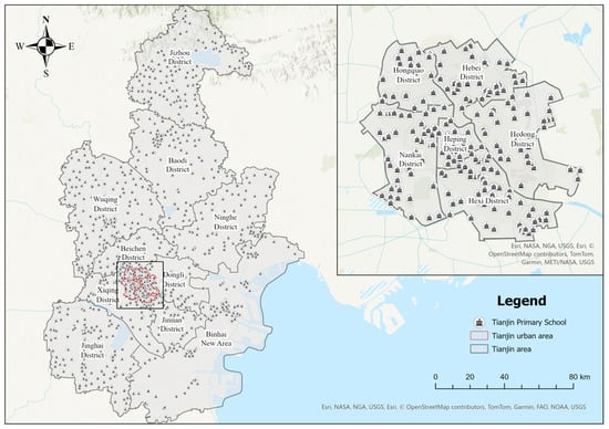
Figure 1.
Stady Area and Distribution of Existing Primary School Facilities.
2.2. Research Framework
This study involves three main steps: (1) Multi-source data collection and preprocessing, constructing a primary and secondary indicator system for educational facility siting. Seventeen types of data—such as healthcare services, dining, and transportation—were collected and partially analyzed for correlation. (2) Model construction and evaluation, where multiple machine learning algorithms were compared and assessed. The best-performing ensemble model was then used to rank feature importance, further quantified using SHAP (SHapley Additive exPlanations). (3) Prediction and site selection, involving initial suitability analysis, comparison with existing educational facilities, and identification of priority areas through secondary filtering based on the population of school-aged children (aged 5–14) and school-to-population ratios. A final recommendation was made based on the combined outputs of RF and XGBoost models. The research framework is illustrated in Figure 2.
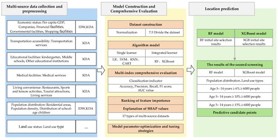
Figure 2.
Research framework.
2.3. Data Sources and Processing
The location selection of educational facilities is influenced by multiple factors. Solving this problem requires various measurement indicators. Common spatial analysis methods include kernel density analysis (KDA) and inverse distance weighted (IDW) interpolation.
KDA is a spatial data analysis technique used to estimate the spatial distribution density of point data. The principle involves using a smoothing kernel function to calculate the influence of each point on its surrounding area. These influences are then superimposed to create a continuous density surface [14]. The theoretical formula is as follows:
Here, f(x) is the estimated density value at location x; n is the number of input points; h is the bandwidth, which determines the smoothness of the kernel function (i.e., the spatial extent considered when estimating density); d is the dimensionality of the data (usually 2 in geographic information systems, representing planar space); and K() is the kernel function, which is a symmetric probability density function.
IDW interpolation is a spatial interpolation method used to estimate the attribute values of unknown points based on the known values of surrounding points. Its core assumption is that the value of the point to be interpolated is determined by nearby known points, using an inverse distance weighted average. In other words, the closer a known point is, the greater its influence on the result [15]. The basic formula is as follows:
Here, Z0 represents the estimated attribute value at the unknown point; Zi represents the attribute value of the known point i; di is the distance from the unknown point to the known point i; p is the power parameter, which determines the influence of the inverse distance on the weighting. The value of p is typically between 1 and 3. n denotes the number of known points involved in the interpolation.
2.4. Construction of Indicator System
The key factors influencing the siting of educational facilities include the presence of a nearby school-age population, the level of economic development at potential sites, quality of life, availability of medical support services, and transportation convenience. We classified the primary factors affecting school siting into seven categories: population distribution, economic status, quality of life, educational infrastructure, medical facilities, transportation accessibility, and topographic conditions. In addition, 17 secondary indicators were identified: Gross Domestic Product (GDP), business establishments, financial institutions, government agencies, shopping centers, residential areas, transportation services, middle schools, kindergartens, other educational institutions, medical services, dining, recreational facilities, tourist attractions, life services, population density, school-age population (ages 5–14), and land use types [16]. The selection of the 17 types of characteristic variables adopted in this study was mainly based on two aspects: Firstly, theoretical basis, referring to the “15 min living circle” and the theory of spatial accessibility [17], emphasizing the significant role of population density, transportation services and the distribution of public facilities in the location selection of educational facilities; Secondly, data availability, relying on the Tianjin Open Data Platform, POI data and the seventh national population census data, ensuring the systematicness and accessibility of the characteristic data. These are listed in Table 1.

Table 1.
Sources and processing of data.
Economic Status: Per capita GDP has a positive impact on the allocation of educational resources. Generally, residents in regions with higher GDP tend to demand higher-quality educational services. Additionally, the distribution of companies, financial institutions, and government agencies indicates employment opportunities and population density, which influence school size and supporting facilities. Shopping venues provide convenience for students’ daily lives but may cause traffic congestion.
Transportation Accessibility: Convenient public transportation and a well-planned road network improve school accessibility, reduce commuting time costs and traffic risks for teachers and students. Efficient transportation systems also promote home-school interactions, facilitate educational resource sharing, and enhance the service capacity of educational facilities.
Educational Facilities: Proximity to kindergartens creates advantages for early childhood education continuity and helps students transition naturally into primary schools. Locating near middle schools facilitates resource sharing, enhancing educational effectiveness. The distribution of other educational institutions enriches after-school resources; however, excessive concentration can lead to traffic congestion. Therefore, when siting primary schools, the spatial relationships among various educational facilities and their combined effects must be considered to ensure educational quality and meet student development needs.
Medical Facilities: Proximity to medical resources enables on-campus emergency healthcare, shortening response times to sudden health incidents and improving health and safety protections for teachers and students. Balanced regional public service facilities are key considerations in primary school siting and education resource allocation.
Living Convenience: Reasonable arrangements of dining facilities provide convenience for student meals. Appropriately located sports and recreational venues meet after-school quality development needs. Tourist attractions offer resources for educational practice. Living service facilities, such as supermarkets, pharmacies, and bookstores, support daily school operations and student life.
Population Distribution: Uneven population distribution leads to imbalances in supply and demand for educational facilities. It is crucial to consider population density and distribution when planning these facilities. The number of local children reflects the demand level for educational facilities.
Land Use Status: Land use types are fundamental spatial factors affecting primary school site selection. Residential land (R category) is preferred due to population agglomeration effects, followed by public service facility land (A category). Industrial land (M category) and storage land (W category)—potential pollution sources—must be strictly avoided.
3. Methodology
3.1. Single Learning Models
3.1.1. Logistic Regression (LR)
Logistic Regression is a supervised learning algorithm used for classification tasks. It constructs a linear decision boundary and applies a Sigmoid function to map the output to a probability between 0 and 1, making it suitable for both binary and multi-class classification. The core idea is to maximize the likelihood function, with parameters optimized using gradient descent or other methods [18].
3.1.2. Support Vector Machine (SVM)
Support Vector Machine is a supervised learning model that seeks to find the hyperplane with the maximum margin to achieve classification or regression. For nonlinear problems, it uses kernel functions to map data into a higher-dimensional space and constructs a linear decision boundary there. The objective is to minimize structural risk and enhance predictive performance [19].
3.1.3. K-Nearest Neighbors (KNN)
K-Nearest Neighbors is an instance-based supervised learning algorithm. It calculates the distance (e.g., Euclidean distance) between the test sample and all samples in the training set, selects the K nearest neighbors, and predicts the label based on majority voting or weighted averaging. The algorithm requires no explicit training and is categorized as a “lazy learning” method [20].
3.1.4. Classification and Regression Tree (CART)
CART is a decision tree algorithm that constructs a binary tree using recursive binary splitting. It can be used for both classification and regression tasks. For classification, it selects features based on minimizing the Gini index, while for regression, it minimizes the squared error. Tree complexity is managed through pruning [21].
3.2. Ensemble Learning Models
3.2.1. Random Forest (RF)
Random Forest is an ensemble learning method that generates multiple decision trees through bootstrap sampling. Each tree is trained on a randomly selected subset of features. The final prediction is obtained by majority voting (for classification) or averaging (for regression). This approach effectively reduces overfitting and enhances model stability [22].
3.2.2. Extreme Gradient Boosting (XGBoost)
XGBoost, also known as Extreme Gradient Boosting, is an ensemble algorithm based on gradient-boosted decision trees. It builds trees iteratively, fitting the residuals of the current model at each step, and introduces regularization terms to prevent overfitting. Its core optimizations include a sparsity-aware algorithm, weighted quantile sketch, and cache optimization, making it well-suited for large-scale datasets [23].
3.3. SHAP (SHapley Additive exPlanations)
SHAP values originate from cooperative game theory. They fairly allocate the difference between a model’s prediction and a baseline (e.g., average prediction) to each input feature, providing a unified measure of feature importance. The SHAP value for a feature represents its marginal contribution to the prediction, calculated across all possible feature combinations [24].
3.4. Hyperparameter Settings and Tuning Strategies
To ensure that different algorithms achieve robust generalization performance under comparable conditions, this study provides the following explanations regarding the key hyperparameters and tuning procedures of each model, as shown in Table 2. We first divide the dataset into a training set and a test set in a 7:3 ratio (random_state = 42). On the training set, we implement systematic parameter optimization using grid search combined with 10-fold cross-validation to ensure the robustness and generalization ability of the results. Specifically, for logistic regression (LR), we search for the regularization strength C ∈ {0.1, 1, 10} and set max_iter to 1000; for support vector machine (SVM), we simultaneously search for the kernel function type {linear, rbf} and the regularization parameter C ∈ {0.1, 1, 10}; for K-nearest neighbors (KNN), we jointly optimize on the neighborhood number n_neighbors ∈ {3, 5, 7} and the weight scheme {uniform, distance}; for CART decision tree, we search for max_depth ∈ {None, 5, 10} and min_samples_split ∈ {2, 5} to control the granularity and complexity of the tree; for random forest (RF), we tune parameters on the number of base learners n_estimators ∈ {100, 200}, max_depth ∈ {5, 10}, and min_samples_split ∈ {2, 5} to balance bias-variance; for XGBoost, we set a grid around the learning rate learning_rate ∈ {0.05, 0.1}, sub-sampling rate subsample ∈ {0.8, 1.0}, and column sampling rate colsample_bytree ∈ {0.8, 1.0} to enhance the fitting ability for non-linear and feature interactions and suppress overfitting. The optimal combinations obtained based on the above process are as follows: LR’s C = 1; SVM’s C = 10, with the kernel function being rbf; KNN’s n_neighbors = 3, weights = distance; CART’s max_depth = None, min_samples_split = 2; RF’s n_estimators = 100, max_depth = 10, min_samples_split = 2; XGBoost’s learning_rate = 0.1, subsample = 0.8, colsample_bytree = 1.0.
Table 2.
Hyperparameter tuning ranges and optimal values of different models.
3.5. Model Performance Evaluation Metrics
In binary classification tasks, model predictions can result in four outcomes: the number of correctly predicted positive samples (True Positives, TP), correctly predicted negative samples (True Negatives, TN), incorrectly predicted positive samples (False Positives, FP), and incorrectly predicted negative samples (False Negatives, FN). Evaluation metrics are defined based on these outcomes, as follows:
Accuracy refers to the proportion of all correctly predicted samples—both true positives and true negatives—relative to the total number of samples. It reflects the overall correctness of the model’s predictions.
Precision is the proportion of correctly predicted positive samples among all samples that the model classified as positive. It indicates how reliable the model’s positive predictions are.
Recall is the proportion of actual positive samples that are correctly predicted as positive by the model.
F1 Score is the harmonic mean of precision and recall, used to comprehensively evaluate both the precision and recall of a model. The formula is as follows:
Area Under the Curve (AUC) refers to the area under the Receiver Operating Characteristic (ROC) curve. This curve illustrates the relationship between the true positive rate (TPR) and the false positive rate (FPR) across different classification thresholds.
4. Experiment on Educational Facility Site Selection
4.1. Construction of the Educational Facility Site Selection Model
Data spatial matching was conducted using a fine grid scale of 500 m × 500 m (based on the service radius of educational facilities and a 15 min walking distance for school-age children) [25]. For each grid cell, quantitative values of secondary indicators for each main influencing factor (see Table 1) were statistically calculated to obtain a feature set from multi-source data. The study area was divided into grids using the fishnet tool in ArcGIS, resulting in 48,721 valid grids. To avoid overlap between the training and prediction sets, multi-source data for Tianjin City were filtered and sampled. According to an equal ratio of positive and negative samples, 2120 grids were randomly selected from the 48,721 valid grids as the sample training set. Grids containing educational facilities were labeled as positive samples, while those without were labeled as negative samples; the positive and negative training samples each numbered 1060. Whether a grid contained a primary school was the dependent variable, while statistical values of 17 feature sets, such as medical facility services, catering, and transportation facility services, served as independent variables. The sample dataset was randomly split into 70% training set and 30% validation set. Apart from the dataset used for model training, the remaining grid data were used as the final test set. When constructing the predictive models using six classification algorithms—LR, SVM, KNN, CART, RF, and XGBoost—10-fold cross-validation was employed to improve model reliability and generalization ability. During model building, features strongly related to educational facility site selection, such as population density, transportation facility services, and distribution of other educational institutions, were selected based on an in-depth analysis of site selection influencing mechanisms.
4.2. Comprehensive Multi-Metric Evaluation
After model construction and training, to comprehensively and objectively evaluate the performance of each classification algorithm in predicting the suitability of primary school site selection, this study used five core metrics: Accuracy, Precision, Recall, F1 score, and AUC. As shown in Figure 3, ensemble learning algorithms represented by RF and XGBoost generally outperformed the four single learners (LR, SVM, KNN, and CART). Quantitative evaluation showed that the average values of overall performance metrics (Accuracy/Precision/Recall/F1/AUC) for single learners were around 0.80, while all metrics for ensemble learners exceeded the 0.80 threshold. Specifically, the accuracies of RF and XGBoost were 0.851 and 0.888, respectively. In terms of Precision, F1 score, and AUC, XGBoost slightly outperformed RF; however, RF showed a marginally higher Recall than XGBoost.
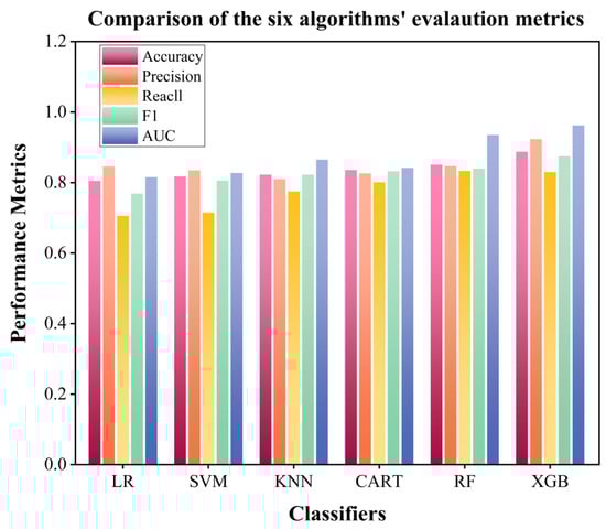
Figure 3.
Comparison of evaluation metrics for six algorithms.
4.3. Feature Importance Ranking
RF and XGBoost models each have advantages and disadvantages across the five evaluation metrics. We compared the ability of these two models to rank feature importance. To clearly present the results, the top five features ranked by each model were selected for analysis. The output is shown in Figure 4.
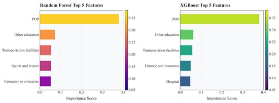
Figure 4.
Ranking of feature importance across multiple features.
In the decision-making process for primary school site selection, the ranking of feature importance reveals the interaction between social demand and resource allocation. Specifically, population density has the greatest impact on primary school site selection, as areas with high population density generally have a higher concentration of school-age children, which aligns with the spatial principle of matching educational facility supply to population distribution. The next most important feature is the distribution of other educational institutions. This may relate to the influence of other educational demands; areas dense with training institutions often reflect parents’ high emphasis on education, which can indirectly promote the coordinated layout of basic education facilities and form an educational agglomeration effect. Lastly, transportation facility services also demonstrate significant importance. This indicates that accessibility plays a key role in public service facility planning. Convenient transportation not only reduces students’ commuting costs but also improves school coverage efficiency by shortening service distances. It is noteworthy that the spatial distribution of these three types of features differs significantly: population density dominates site selection demand in urban core areas; clusters of other educational institutions are mostly located in emerging residential zones; and transportation hubs serve as important bases for school layout in suburban areas. Based on these findings, future basic education planning should implement differentiated strategies. In densely populated areas, the priority should be expanding existing schools. In regions dense with educational institutions, integrated community models combining training and basic education can be explored. Meanwhile, near transportation hubs, optimizing inter-school transportation connectivity systems is necessary.
4.4. SHAP Explanation of the XGBoost Model
Given that XGBoost exhibits relatively superior overall performance in key evaluation metrics, such as precision (0.924) and AUC value (0.962), it establishes a more robust model foundation for mechanism analysis. While the feature importance rankings of Random Forest (RF) and XGBoost are highly consistent—identifying population density, other educational institutions, and transportation facilities as the top three features—XGBoost demonstrates distinct advantages in quantifying the directional contributions of features and capturing non-linear interaction effects. This capability is essential for elucidating the spatial collaborative configuration mechanism of the “15 min living circle.” To further interpret the predictive outcomes of the XGBoost model, this study employs a game theory-based SHAP method (Figure 5) to systematically quantify the contributions of various features to the suitability scores for primary school site selection. The analysis shows that the mean SHAP value of population density (POP) is 1.320, significantly higher than other factors, highlighting the core role of the spatial matching principle between population and educational resources in public facility planning. This clearly reflects that the distribution of school-age population fundamentally constrains educational resource allocation.
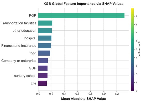
Figure 5.
SHAP-based interpretation of the XGBoost model.
Accessibility of transportation facilities (Transportation facilities, SHAP = 0.217) and the distribution of other educational institutions (Other education, SHAP = 0.210) rank second and third in importance. Transportation facilities reduce commuting costs and improve school service coverage efficiency. Meanwhile, the agglomeration of educational institutions can indirectly promote the coordinated layout of basic education facilities and bring scale economies.
Contributions from medical facilities (Hospital, SHAP = 0.204) and financial services (Finance and Insurance, SHAP = 0.198) are also noteworthy. Their significant contributions reveal a multidimensional synergy among public service facilities. Medical resources ensure children’s health and safety, while financial outlets support household consumption capacity. Both are core elements of a high-quality living environment. This finding indicates that when selecting educational facility sites, the demand for non-educational public service facilities must also be considered.
Economic foundation (GDP, SHAP = 0.145) and distribution of preschool institutions (Nursery school, SHAP = 0.144) have relatively lower direct contributions but embody key policy implications in their positive influence mechanisms. GDP’s indirect support reflects regional fiscal capacity as a core indicator. The GDP level underpins the sustainable supply of educational resources through government education investment (e.g., per-student funding, teacher allocation), exerting more influence at the macro-policy level rather than micro-level site decisions. The spatial coupling between preschool and primary education is clearly demonstrated by the spatial distribution of kindergartens (SHAP = 0.144), highlighting the collaborative facility needs under the “15 min living circle” planning framework and the requirement for spatial continuity. Notably, the direct contribution of life service facilities (Life, SHAP = 0.134) is relatively small, suggesting its impact on site selection may be indirect via other factors.
4.5. Model Parameter Optimization and Tuning Strategies
4.5.1. Purpose and Methodology of Tuning
To enhance the prediction accuracy of ensemble learning models for evaluating the suitability of educational facility site selection, this study conducted systematic parameter optimization for algorithms such as RF and XGBoost. The core objective of parameter tuning is to balance model fitting ability and generalization capacity, thereby avoiding overfitting or underfitting. Considering the nonlinear characteristics and interaction effects of multi-source data, a grid search combined with 10-fold cross-validation was employed. This approach ensures the reliability of the tuning results while maintaining computational efficiency. Evaluation metrics include Accuracy, Precision, Recall, F1 score, and AUC.
4.5.2. Parameter Ranges and Tuning Strategy
For each model, the search space for key hyperparameters was defined based on literature experience [22,26,27] and preliminary experimental results:
RF: Optimization focused on the number of decision trees (n_estimators), maximum tree depth (max_depth), and the minimum number of samples required to split a node (min_samples_split). The search range for n_estimators was set to [50, 200], balancing model complexity and computational cost; max_depth was limited to [5, 15] to prevent overfitting; and min_samples_split was set between [2, 10] to control tree granularity.
XGBoost: Key parameters include the learning rate (learning_rate), column subsampling rate (colsample_bytree), and row subsampling rate (subsample). The learning_rate was set between [0.01, 0.3] to enhance model robustness by reducing step size. Both colsample_bytree and subsample were tuned within [0.5, 1.0] to introduce randomness and improve generalization.
Single Model Comparison: For baseline models such as LR and SVM, parameter tuning was also conducted. For LR, the regularization parameter C was tuned within [0.1, 10]. For SVM, the kernel function was selected from linear or radial basis function (RBF), and the penalty parameter C was optimized accordingly.
4.5.3. Tuning Process and Key Results
The optimization process was implemented using Python’s scikit-learn (Version 1.4.1) and XGBoost libraries, employing parallel computing to enhance search efficiency. Taking the RF model as an example, after conducting 10-fold cross-validation, the optimal parameter combination was found to be n_estimators = 100, max_depth = 10, and min_samples_split = 2, resulting in a recall value of 0.833 on the validation set, which represents an improvement of 8.2% over the default parameters.
For XGBoost, the optimal parameters were identified as learning_rate = 0.1, colsample_bytree = 1.0, and subsample = 0.8, corresponding to a precision value of 0.924 and an AUC value of 0.962, demonstrating a strong capacity for fitting complex feature interactions.
During the tuning process, models such as RF, XGBoost, SVM, and KNN showed notable performance improvements, as shown in Table 3. In contrast, LR and CART models exhibited no significant improvements, as their optimal parameters were either identical to or very close to the default settings.
Table 3.
Hyperparameter Optimization Results and Performance Gains.
4.5.4. Result Analysis and Model Advantages
The tuning results indicate that ensemble learning models (RF and XGBoost) significantly outperform single models in overall performance. XGBoost demonstrates outstanding performance in terms of precision (0.924) and AUC, benefiting from its gradient boosting mechanism, which dynamically adjusts feature weights. The RF model performs slightly better in recall (0.833), which can be attributed to its robustness to noise introduced by random sampling. In contrast, single models such as LR show weaker performance due to the limitations of linear assumptions, which struggle to capture the nonlinear relationships inherent in multi-source data. While KNN and CART perform well in local fitting, the lack of ensemble strategies results in lower generalization stability.
Feature importance analysis shows that the tuned models more accurately identify key influencing factors: population density, transportation facility services, and the distribution of other educational institutions receive significantly higher importance scores (Figure 4). This finding aligns with the SHAP-based interpretation results (Figure 5), further validating the interpretability of the optimized models.
5. Prediction Results of Suitability for Primary School Site Selection
5.1. Preliminary Site Selection Results
Following the steps described above, the trained RF and XGBoost models were applied to primary school site selection, yielding preliminary prediction results. During the model discrimination process, the prediction probability threshold was set at 0.5. That is, if a certain grid point was predicted by the model to have an appropriate probability greater than 0.5, it was regarded as a “suitable” location point; otherwise, it was classified as “unsuitable”. This threshold selection followed the commonly used standard for binary classification tasks [26]. The RF model identified 16,946 suitable grid points, while the XGBoost model identified 19,403. These results represent initial predictions; actual planning requires secondary screening combined with factors such as population distribution and land use types.
To verify model reliability, the predicted points were spatially compared with the locations of 1136 existing primary schools in Tianjin. The existing schools have been selected and preserved through long-term practical experience, thus holding practical significance and reference value. Validation results showed that the RF model achieved an accuracy of 84.70%, and the XGBoost model reached 92.41%. This indicates that our models demonstrate good fitting and reliability to some extent, providing a credible foundation for current educational resource allocation. Additionally, these models accurately predict spatial distribution differences in primary schools in Tianjin, proving their ability not only to maintain the advantages of existing layouts but also to precisely analyze the spatial differentiation patterns of regional educational resources.
5.2. Secondary Screening of Site Selection Results
The number of highly suitable locations predicted in the preliminary selection greatly exceeds the number of primary school facilities that Tianjin can feasibly plan and build. Therefore, a secondary screening is necessary, based on factors such as the number of children aged 0–14 in each subdistrict and township according to the Seventh National Population Census, and land use types.
According to the “Design Specifications for Primary and Secondary Schools” (GB 50099-2011) [28] the recommended suitable size for a primary school is 12–36 classes, i.e., approximately 540–1620 students (calculated at 45 students per class). The average number of children aged 0–14 in Tianjin’s subdistricts and townships exceeds 6000. Therefore, we first selected 120 subdistricts and townships where the 0–14 population exceeds 6000.
Furthermore, based on the regulations from the Ministry of Education, Ministry of Housing and Urban-Rural Development, and Ministry of Natural Resources in the “Urban Residential Area Planning and Design Standard” (GB50180-2018) [29], primary schools must be configured as service facilities within a 10 min living circle in residential areas. The 10 min living circle is an important part of the 15 min living circle, and reasonable layout should be fully considered [30]. To make the secondary screening more reasonable, we further selected subdistricts and townships where the proportion of children aged 5–14 reaches 6%, 10%, and 15%, respectively. When the ratio of the 5–14 population to primary schools reaches 6%, the area is defined as a “low-density education demand zone”; at 10%, as a “medium-density education demand zone”; and at 15%, as a “high-density education demand zone,” as shown in Table 4.
Table 4.
Classification Criteria for Educational Demand Zones in Site Selection.
Using ArcGIS, buffer zone analysis was conducted for 500 m × 500 m service areas around educational facilities. Existing primary school grids in Tianjin were excluded based on location attributes, as shown in Figure 6. The selected subdistricts and townships filtered by the three 5–14 age group suitability levels were analyzed to provide references for local governments and related enterprises to plan new educational facilities, better aligning with the 15 min living circle planning concept.
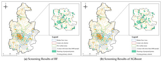
Figure 6.
Preliminary Secondary Site Selection Results Based on RF and XGBoost.
5.2.1. Screening Results for Low-Density Educational Demand Zones
The spatial distribution analysis of “school-age children” (children aged 5–14) across 120 streets and towns, based on the selection of RF and XGBoost models, identified 1026 and 1069 grid units with high site suitability in low-density education demand areas. As illustrated in Figure 7, the spatial distribution of grid points selected by both models exhibits regional clustering characteristics, primarily concentrated in the six urban districts, western Dongli District, Jinnan District, Xiqing District, Jinghai District, Baodi District, and Binhai New Area. Although these regions are categorized as low-density education demand areas (indicating that the existing school configuration is relatively adequate or the demand pressure is minimal), the spatial aggregation of high-suitability grid points reveals potential opportunities for optimizing educational resources. This can serve as strategic reserve locations for future population growth or service capacity upgrades. In the secondary site selection phase, priority is given to overlapping results from the models to enhance decision robustness.
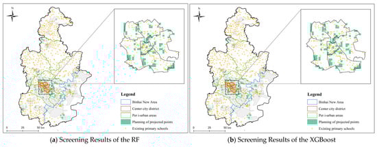
Figure 7.
Screening Results for Low-Density Educational Demand Zones.
5.2.2. Screening Results for Medium-Density Educational Demand Zones
Based on the selection results from the RF and XGBoost models, high-suitability site grid units were identified in medium-density education demand areas, with the RF model identifying 622 units and the XGBoost model identifying 643 units, as shown in Figure 8. These areas experience moderate pressure regarding the educational needs of school-age children, indicating an optimizable supply–demand gap between the existing school service capacity and the population size. The spatial distribution of grid points selected by both models exhibits significant regional concentration, primarily located in Jinnan District, Xiqing District, Dongli District, Baodi District, and Binhai New Area. As a key optimization target for the construction of the “15 min living circle,” this region requires the addition of educational facilities to alleviate the pressure on degree supply while enhancing spatial service equity. Therefore, combining the overlapping results from the models, Baoping Street in Baodi District and Huaming Street in Dongli District have been selected as priority candidate areas for secondary site selection.
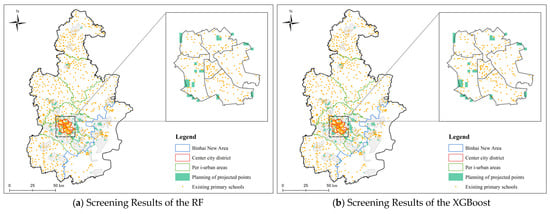
Figure 8.
Screening Results for Medium -Density Educational Demand Zones.
5.2.3. Screening Results for High-Density Educational Demand Zones
Based on the selection results from the RF and XGBoost models, 267 and 277 high-suitability site grid points were identified in high-density education demand areas, respectively, as illustrated in Figure 9. This region exhibits a severe imbalance between educational demand and supply, highlighting the critical contradiction between the overloaded service radius of existing schools and the acute shortage of available school places. The intersecting grid points from both models are primarily distributed in Jinghai District, Xiqing District, and Binhai New Area. As an urgent target for transformation in the construction of the “15 min living circle,” it is essential to rapidly alleviate enrollment pressure through the establishment of new facilities. Given this spatial distribution characteristic, areas such as Gulin Street in Binhai New Area and Liqizhuang Town in Xiqing District demonstrate a high match between educational demand and spatial suitability, warranting priority in site selection.
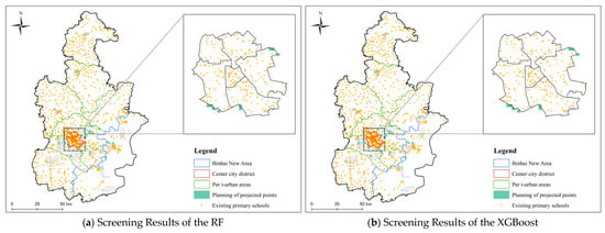
Figure 9.
Screening Results for High-Density Educational Demand Zones.
5.3. Conclusions and Recommendations for Secondary Site Selection
For secondary site selection, based on the overlapping results from the RF and XGBoost models, we draw the following conclusions and recommendations:
(1) A total of 12 subdistricts and townships are identified as priority areas for primary school construction: Baoping Subdistrict in Baodi District; Huaming Subdistrict in Dongli District; Zhongbei Town, Zhangjiawo Town, Liqizhuang Town, and Dasi Town in Xiqing District; Jinghai Town in Jinghai District; Xianshuigu Town in Jinnan District; and Hujayuan Subdistrict, Xinbei Subdistrict, Hangzhou Road Subdistrict, and Gulin Subdistrict in Binhai New Area, as shown in Figure 10a. By integrating the RF model’s capacity to capture spatial heterogeneity and the XGBoost model’s strength in nonlinear multivariate fitting, the selected sites effectively meet key requirements such as population density and transportation accessibility. For instance, the Gulin Subdistrict of Binhai New Area, being a rapidly developing area, has witnessed signifi cant population inflow in recent years, resulting in a rapid increase in the number of school-age children. However, the existing primary schools are insufficient to cover this demand, leading to concentrated educational pressure. Through model predictions, we not only identified these demand hotspots but also further combined land use types and population structure data to propose prioritizing the establishment of new schools in these areas.
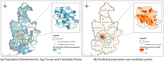
Figure 10.
Predicted Candidate Sites in Tianjin.
(2) Combining the SHAP results, it can be seen that population density has always been a crucial factor in determining the location of schools. To further incorporate the perspective of future urban development into the selection framework, we integrated the population prediction data for the 2030 km grid under the Shared Socioeconomic Pathways (SSPs) [31]. On one hand, the current population distribution can reveal the current demand for educational resources; on the other hand, the future population trend determines the continued applicability of the facility layout. By superimposing the population prediction results for 2030, we can ensure that the candidate locations not only meet the current supply–demand balance but also have forward-looking and sustainable characteristics, avoiding the problem of insufficient timeliness due to relying solely on current data. As shown in Figure 10b, we superimposed the population prediction with the secondary selection results. The results indicate that the secondary selection results show a high degree of consistency with the future population hotspots. This synergy effect indicates that these locations are not only suitable under the current conditions but also adaptable to future population structure changes, thereby providing support for the sustainable educational planning of the “15 min living circle”. The integration of future population data enhances the time scalability of the model and provides a more robust foundation for long-term educational infrastructure planning.
(3) During the site selection process, full consideration should be given to the living habits and cultural backgrounds of local children and adolescents to ensure the provision of primary education services that meet their needs. Meanwhile, a sound regulatory mechanism should be established to oversee the entire process of planning, construction, and operation of primary education facilities. This includes ensuring that school locations meet safety standards, that educational resources are allocated reasonably, and that the quality of education is continuously improved—ultimately ensuring the standardized and effective operation of schools.
6. Discussion
6.1. Theoretical and Practical Significance of the Findings
This study integrates multi-source big data with ensemble learning models to establish a refined evaluation framework for primary school site selection in Tianjin, providing a scientific basis for the optimized allocation of educational resources. The findings indicate that population density, the distribution of other educational institutions, and transportation accessibility are the core factors influencing site selection—highly consistent with the “15 min living circle” concept. This confirms the critical role of spatial supply–demand matching in planning. The model’s prediction results align closely with existing facilities (RF: 84.70%; XGBoost: 92.41%), demonstrating the reliability of the intersection-based approach. The ensemble models effectively overcome the limitations of single algorithms, offering more robust decision support for educational facility planning.
From a methodological perspective, ensemble learning models exhibit notable advantages, particularly in feature importance ranking and predictive accuracy. For instance, the XGBoost model, through SHAP value analysis, quantified the importance of population density (1.320), transportation facilities (0.217), and other educational institutions (0.210), providing an interpretable foundation for policy-making. Compared to traditional GIS spatial analysis or Analytic Hierarchy Process (AHP), this approach better captures complex multivariate nonlinear relationships, significantly improving model reliability.
From an international perspective, the results of this study show certain commonalities with similar studies conducted in China, Europe, and North America. For instance, the “compact city” concept in Europe [32] and the research on school accessibility and equity in North America [33] both emphasize the decisive role of population density and transportation conditions in the location of educational institutions. However, unlike traditional methods that rely on GIS analysis or multi-criteria approaches, this study employs an integrated learning model, which better captures nonlinear relationships and feature interactions, resulting in significantly improved prediction accuracy.
6.2. Limitations and Future Research Directions
Despite achieving phased results, this study has several limitations.
First, the data dimensions require expansion. Among the 17 categories of integrated multi-source data, key socioeconomic dynamics (e.g., household income, cultural preferences) and real-time traffic flow data are missing. This limits the model’s ability to capture the heterogeneity of educational demand.
Second, due to computational constraints, hyperparameter tuning did not explore higher-order interaction effects (e.g., between RF’s ‘max_features’ and ‘n_estimators’).
Third, the secondary screening indicators are incomplete. Relying solely on the 5–14 age population ratio excludes subjective factors like educational quality and parental preferences, which may lead to deviations between the site selection results and actual needs.
Future research can deepen in the following areas:
(1) Expand data dimensions by integrating emerging data sources such as mobile signaling and social media to build a multidimensional evaluation system covering “demand–supply–environment”.
(2) Introduce Bayesian optimization or genetic algorithms for more efficient search in high-dimensional parameter spaces, incorporating domain knowledge to define prior distributions for parameters and further improving tuning efficiency.
(3) Develop a spatiotemporal dynamic model and combine population prediction data to optimize the location selection strategy. Future research should incorporate predictive population models and urban planning data into the framework, such as the projected growth of the school-age population, the development trends of the built-up areas and new urban districts, in order to enhance the forward-looking and long-term adaptability of the site selection model.
6.3. Practical Application Suggestions
The location model and its output results constructed in this study can provide a scientific and operational decision support tool for local authorities in educational facility planning. Specifically, the multi-level outcomes generated by the model, including high-suitability location grids, priority ranking of streets and towns, and SHAP explanations of key driving factors, can be directly integrated into the existing workflow of urban planning. Firstly, the planning department can use the GIS platform to overlay the initial location results with the national spatial planning, current land use status, and detailed control planning to quickly identify potential plots that are both in line with the model’s predictions and have actual construction conditions, guiding the reservation and allocation of educational land. Secondly, for the high-priority streets and towns selected in the second round (such as Baoping Street in Baodi District and Huaming Street in Dongli District), the authorities can formulate differentiated construction strategies based on the key factors revealed by the SHAP values (such as population density and traffic accessibility): prioritize new construction projects in areas with high population concentration but facility shortages, and optimize bus routes around transportation hubs to improve service coverage efficiency. At the same time, overlaying future population prediction results with the secondary location results not only validates the rationality of the current results but also provides planners with references for future population hotspots. This combination approach effectively avoids the problem of timeliness deficiency caused by relying solely on the current situation, enabling educational facility location to take into account both current needs and future trends. More importantly, what this study provides is not just a static location map but a dynamic assessment framework. By regularly updating multi-source data such as population and POIs and re-running the model, local governments can continuously monitor the spatio-temporal changes in the supply and demand of educational facilities, make rolling adjustments to planning schemes, and evaluate their effectiveness, thereby transforming from “one-time planning” to “continuous governance” and promoting the refinement and dynamic optimization of the layout of educational resources.
7. Conclusions
This study selects Tianjin as the research area, integrating multi-source geospatial big data at a 500 m grid resolution to construct a suitability evaluation model for primary school site selection based on ensemble learning. The study yields both preliminary and secondary screening results. The main conclusions are as follows:
(1) The comprehensive evaluation metrics of the two ensemble learning models, RF and XGBoost, including accuracy, precision, recall, F1 score, and AUC value, are all around 85%, outperforming four individual learning models such as LR and SVM. More importantly, the model predictions demonstrate a fitting degree of 84.70% and 92.41% with the existing primary school educational facilities, effectively indicating that these models perform well and can accurately predict optimal site selections.
(2) Primary school site selection is closely related to population density, other educational institutions, transportation services, and medical services—these are the four key factors determining spatial distribution. SHAP results indicate that “population density,” “other educational institutions,” and “transportation services” are the most influential on suitability.
(3) Compared to previous studies, this research provides a more detailed classification of influencing factors, examines secondary features, and ranks the importance of each, offering references for planning other types of facilities.
(4) Preliminary site selection results in Tianjin show that highly suitable areas are concentrated in the city center and surrounding regions. By further screening subdistricts and townships with varying levels of school-age children and combining the overlapping results of RF and XGBoost models, the following priority areas are identified: Baoping Subdistrict in Baodi District; Huaming Subdistrict in Dongli District; Zhongbei Town, Zhangjiawo Town, Liqizhuang Town, and Dasi Town in Xiqing District; Jinghai Town in Jinghai District; Xianshuigu Town in Jinnan District; and Hujayuan, Xinbei, Hangzhou Road Subdistrict, and Gulin Subdistricts in Binhai New Area. Deploying educational infrastructure in these areas will significantly enhance the spatial equity and service quality of primary education provision.
Author Contributions
Conceptualization, Zhenhui Sun; methodology, Ying Xu and Zhenhui Sun; validation, Junjie Ning; visualization, Yufan Wang and Yunxiao Sun; writing—original draft preparation, Zhenhui Sun and Ying Xu; writing—review and editing, Zhenhui Sun and Ying Xu; funding acquisition, Zhenhui Sun. All authors have read and agreed to the published version of the manuscript.
Funding
This research was supported by the 2021 Tianjin Educational Science Planning Youth General Project (Project No. EHE210290), titled “Research on the Spatial Structure and Optimization Strategies of Teacher Mobility in Compulsory Education Between Tianjin and Binhai under the Perspective of Quality and Equity”.
Data Availability Statement
The data is public data.
Acknowledgments
We appreciate the constructive comments and suggestions from the reviewers, that helped improve the quality of this manuscript.
Conflicts of Interest
The authors declare no conflicts of interest.
References
- Moreno, C.; Allam, Z.; Chabaud, D.; Gall, C.; Pratlong, F. Introducing the “15-Minute City”: Sustainability, Resilience and Place Identity in Future Post-Pandemic Cities. Smart Cities 2021, 4, 93–111. [Google Scholar] [CrossRef]
- Chai, Y.W.; Li, C.J. Urban Life Cycle Planning: From Research to Practice. City Plan. Rev. 2019, 43, 9–16+60. [Google Scholar]
- Huang, A.; Xu, Y.; Zhang, Y.; Lu, L.; Liu, C.; Sun, P.; Liu, Q. A Spatial Equilibrium Evaluation of Primary Education Services Based on Living Circle Models: A Case Study within the City of Zhangjiakou, Hebei Province, China. Land 2022, 11, 1994. [Google Scholar] [CrossRef]
- Wu, H.; Wang, L.; Zhang, Z.; Gao, J. Analysis and Optimization of 15-Minute Community Life Circle Based on Supply and Demand Matching: A Case Study of Shanghai. PLoS ONE 2021, 16, e0256904. [Google Scholar] [CrossRef]
- Sakti, A.D.; Rahadianto, M.A.E.; Pradhan, B.; Muhammad, H.N.; Andani, I.G.A.; Sarli, P.W.; Abdillah, M.R.; Anggraini, T.S.; Purnomo, A.D.; Ridwana, R. School Location Analysis by Integrating the Accessibility, Natural and Biological Hazards to Support Equal Access to Education. ISPRS Int. J. Geo-Inf. 2021, 11, 12. [Google Scholar] [CrossRef]
- Al-Sabbagh, T.A. Gis Location-Allocation Models in Improving Accessibility to Primary Schools in Mansura City-Egypt. GeoJournal 2022, 87, 1009–1026. [Google Scholar] [CrossRef]
- Barbara, M.; Rey, D.; Akbarnezhad, A. Optimizing Location of New Public Schools in Town Planning Considering Supply and Demand. J. Urban Plan. Dev. 2021, 147, 04021057. [Google Scholar] [CrossRef]
- Prasetyo, D.H.; Mohamad, J.; Fauzi, R. A Gis-Based Multi-Criteria Decision Analysis Approach for Public School Site Selection in Surabaya, Indonesia. Geomatica 2018, 72, 69–84. [Google Scholar] [CrossRef]
- Lotfi, R.; Pilehforooshha, P.; Karimi, M. A Multi-Objective Optimization Model for School Location-Allocation Coupling Demographic Changes. J. Spat. Sci. 2023, 68, 225–244. [Google Scholar] [CrossRef]
- Chaturvedi, V.; de Vries, W.T. Machine Learning Algorithms for Urban Land Use Planning: A Review. Urban Sci. 2021, 5, 68. [Google Scholar] [CrossRef]
- Zaheer, N.; Hassan, S.-U.; Ali, M.; Shabbir, M. Optimal School Site Selection in Urban Areas Using Deep Neural Networks. J. Ambient. Intell. Humaniz. Comput. 2022, 13, 313–327. [Google Scholar] [CrossRef]
- Huang, J.-C.; Ko, K.-M.; Shu, M.-H.; Hsu, B.-M. Application and Comparison of Several Machine Learning Algorithms and Their Integration Models in Regression Problems. Neural Comput. Appl. 2020, 32, 5461–5469. [Google Scholar] [CrossRef]
- Marino, S.; Zhao, Y.; Zhou, N.; Zhou, Y.; Toga, A.W.; Zhao, L.; Jian, Y.; Yang, Y.; Chen, Y.; Wu, Q. Compressive Big Data Analytics: An Ensemble Meta-Algorithm for High-Dimensional Multisource Datasets. PLoS ONE 2020, 15, e0228520. [Google Scholar] [CrossRef]
- Boumeddane, S.; Hamdad, L.; Haddadou, H.; Dabo-Niang, S. A Kernel Discriminant Analysis for Spatially Dependent Data. Distrib. Parallel Databases 2021, 39, 583–606. [Google Scholar] [CrossRef]
- Zhang, Y.; Zhu, J.; Li, F.; Wang, Y. Site Selection of Elderly Care Facilities Based on Multi-Source Spatial Big Data and Integrated Learning. ISPRS Int. J. Geo-Inf. 2024, 13, 451. [Google Scholar] [CrossRef]
- Shukla, K.; Kumar, P.; Mann, G.S.; Khare, M. Mapping Spatial Distribution of Particulate Matter Using Kriging and Inverse Distance Weighting at Supersites of Megacity Delhi. Sustain. Cities Soc. 2020, 54, 101997. [Google Scholar] [CrossRef]
- Graells-Garrido, E.; Serra-Burriel, F.; Rowe, F.; Cucchietti, F.M.; Reyes, P. A city of cities: Measuring how 15-minutes urban accessibility shapes human mobility in Barcelona. PLoS ONE 2021, 16, e0250080. [Google Scholar] [CrossRef]
- Hastie, T.; Tibshirani, R.; Friedman, J. The Elements of Statistical Learning; Springer: New York, NY, USA, 2009. [Google Scholar]
- Cortes, C.; Vapnik, V. Support-Vector Networks. Mach. Learn. 1995, 20, 273–297. [Google Scholar] [CrossRef]
- Cover, T.; Hart, P. Nearest Neighbor Pattern Classification. IEEE Trans. Inf. Theory 1967, 13, 21–27. [Google Scholar] [CrossRef]
- Wu, X.; Kumar, V.; Ross Quinlan, J.; Ghosh, J.; Yang, Q.; Motoda, H.; McLachlan, G.J.; Ng, A.; Liu, B.; Yu, P.S. Top 10 Algorithms in Data Mining. Knowl. Inf. Syst. 2008, 14, 1–37. [Google Scholar] [CrossRef]
- Breiman, L. Random Forests. Mach. Learn. 2001, 45, 5–32. [Google Scholar] [CrossRef]
- Chen, T.; Guestrin, C. Xgboost: A Scalable Tree Boosting System. In Proceedings of the 22nd ACM SIGKDD International Conference on Knowledge Discovery and Data Mining 2016, San Francisco, CA, USA, 13–17 August 2016. [Google Scholar]
- Sun, Y.; Ai, H.; Li, Y.; Wang, R.; Ma, R. Data-Driven Large-Scale Spatial Planning Framework for Determining Size and Location of Offshore Wind Energy Development: A Case Study of China. Appl. Energy 2024, 367, 123388. [Google Scholar] [CrossRef]
- Sun, Y.; Luo, S. A Study on the Current Situation of Public Service Facilities’ Layout from the Perspective of 15-Minute Communities—Taking Chengdu of Sichuan Province as an Example. Land 2024, 13, 1110. [Google Scholar] [CrossRef]
- Fabian, P. Scikit-Learn: Machine Learning in Python. J. Mach. Learn. Res. 2011, 12, 2825–2830. [Google Scholar]
- Yuliana, H.; Basuki, S.; Hidayat, M.R.; Charisma, A.; Vidyaningtyas, H. Hyperparameter Optimization of Random Forest Algorithm to Enhance Performance Metric Evaluation of 5g Coverage Prediction. Bul. Pos Dan Telekomun. 2024, 22, 75–90. [Google Scholar]
- GB 50099-2011; Code for Design of Primary and Secondary School. Ministry of Housing and Urban-Rural Development of the People’s Republic of China; China Architecture & Building Press: Beijing, China, 2011.
- GB 50180-2018; Standard for Urban Residential Area Planning and Design. Ministry of Housing and Urban-Rural Development of the People’s Republic of China; China Architecture & Building Press: Beijing, China, 2018.
- Wu, W.; Divigalpitiya, P. Availability and Adequacy of Facilities in 15 Minute Community Life Circle Located in Old and New Communities. Smart Cities 2023, 6, 2176–2195. [Google Scholar] [CrossRef]
- Wang, X.; Meng, X.; Long, Y. Projecting 1 km-grid population distributions from 2020 to 2100 globally under shared socioeconomic pathways. Sci. Data 2022, 9, 563. [Google Scholar] [CrossRef]
- Bibri, S.E.; Krogstie, J.; Kärrholm, M. Compact city planning and development: Emerging practices and strategies for achieving the goals of sustainability. Dev. Built Environ. 2020, 4, 100021. [Google Scholar] [CrossRef]
- Villalba, A.; Vila Lladosa, L.; Carot, J.M. Analyzing Patterns of Accessibility to Schools: A Gravitational Metrics Study in València. Aims Math. 2024, 10, 809–825. [Google Scholar] [CrossRef]
Disclaimer/Publisher’s Note: The statements, opinions and data contained in all publications are solely those of the individual author(s) and contributor(s) and not of MDPI and/or the editor(s). MDPI and/or the editor(s) disclaim responsibility for any injury to people or property resulting from any ideas, methods, instructions or products referred to in the content. |
© 2025 by the authors. Published by MDPI on behalf of the International Society for Photogrammetry and Remote Sensing. Licensee MDPI, Basel, Switzerland. This article is an open access article distributed under the terms and conditions of the Creative Commons Attribution (CC BY) license (https://creativecommons.org/licenses/by/4.0/).