Digital Relations in ${\mathbb{Z}}^1$: Discretized Time and Rasterized Lines

Abstract

There is voluminous literature concerning the scope of topological relations that span various embedding spaces from ${\mathbb{R}}^1$ to ${\mathbb{R}}^2$, ${\mathbb{Z}}^2$ , ${\mathbb{S}}^1$ and ${\mathbb{S}}^2$ , and ${\mathbb{T}}^2$. In the case of the ${*}^1$ spaces, those relations have been considered as conceptualizations of both spatial relations and temporal relations. Missing from that list are the set of digital relations that exist within ${\mathbb{Z}}^1$ , representing discretized time, discretized ordered line segments, or discretized linear features as embedding spaces. Discretized time plays an essential role in timeseries data, spatio-temporal information systems, and geo-foundation models where time is represented in layers of consecutive spatial rasters and/or spatial vector objects colloquially referred to as space–time cubes or spatio-temporal stacks. This paper explores the digital relations that exist in ${\mathbb{Z}}^1$ interpreted as a regular topological space under the digital Jordan curve model as well as a folded-over temporal interpretation of that space for use in spatio-temporal information systems and geo-foundation models. The digital Jordan curve model represents the maximum expressive power between discretized objects, making it the ideal paradigm for a decision support system model. It identifies 34 9-intersection relations in ${\mathbb{Z}}^1$ , 42 9-intersection + margin relations in ${\mathbb{Z}}^1$ , and 74 temporal relations in ${\mathbb{Z}}^1$ , utilizing the 9+-intersection, the commercial standard for spatial information systems for querying topological relations. This work creates opportunities for better spatio-temporal reasoning capacity within spatio-temporal stacks and a more direct interface with intuitive language concepts, instrumental for effective utilization of spatial tools. Three use cases are demonstrated in the discussion, representing each of the utilities of ${\mathbb{Z}}^1$ within the spatial data science community.

1. Introduction

In a broad sense, temporal reasoning asserts new relations between events localized in time by facts known about the events themselves [1]. We can think of that in either quantitative terms, such as this event concludes 10 min before the next scheduled event at 9 a.m., or we can think of that in qualitative terms, such as this event happens before that other event. As Naïve Geography opines, topology matters, but metric refines [2]. The same is, in theory, true in time—our temporal language seems to rely on prepositions in many cases to succinctly communicate temporal concepts in our day-to-day life, just as topological relations are used as the basis for prepositional phrases [3,4]. Both of these concepts have been critical to the formation of the field of geographic information science, as geography almost necessarily invokes both space and time simultaneously, either implicitly or explicitly [5,6].

Temporal reasoning, however, can be more rigidly classified [1]. Over the decades of research developing spatial and temporal reasoning, researchers have identified many first-order logic, propositional logic, and reified logic structures for evaluating both spatial and temporal relations. These types of techniques include formalisms such as Allen’s interval algebra [7], the 4-intersection [8], the 9-intersection [9], the dimensionally extended 9-intersection [10], and the region connection calculus [11], amongst others. These types of reasoning structures have become implemented in different software products to answer core questions in modern day applications, but, nevertheless, they do not exhaust all possibilities or all aspects of temporal reasoning [1,12], or even spatial reasoning for that matter [13]. A basic compendium of qualitative relational sets that have been described in the literature is shown in

Table 1. Existing topological relation sets for simple polygons and lines in various spaces.

Space	Lines	Polygons	Polygons/Lines
${\mathbb{R}}^1$	[7]	-	-
${\mathbb{R}}^2$	[14,15]	[8,9,11]	[16]
${\mathbb{S}}^1$	[17]	-	-
${\mathbb{S}}^2$	[14,15] *	[18,19]	[16] *
${\mathbb{Z}}^1$	not identified	-	-
${\mathbb{Z}}^2$	not identified	[20,21,22,23]	not identified
${\mathbb{T}}^1$	not identified	-	-
${\mathbb{T}}^2$	not identified	[24]	not identified

* extended to spherical embedding spaces by default due to negligible change between spherical and planar space with respect to the participating objects

.

${\mathbb{R}}^1$${\mathbb{R}}^2$${\mathbb{S}}^1$${\mathbb{S}}^2$${\mathbb{Z}}^1$${\mathbb{Z}}^2$${\mathbb{T}}^1$${\mathbb{T}}^2$Various embedding spaces are listed in Table 1 that will, in some sense, permeate throughout this manuscript. Most readers will be familiar with ${\mathbb{R}}^1$ and ${\mathbb{R}}^2$ from a rudimentary study of high school algebra and geometry. These spaces represent the one-dimensional real number line and its cross product that embedding spaces typically used to express time (${\mathbb{R}}^1$) and localized geographic space (${\mathbb{R}}^2$). When we consider the Earth’s geoidal surface, a different embedding space is needed. This embedding space is called ${\mathbb{S}}^2$, a sphericalized version of ${\mathbb{R}}^2$, fundamentally similar to the latitudinal and longitudinal reference on Earth. Similarly, we can consider a cyclic real line counterpart, namely ${\mathbb{S}}^1$. For example, if we treated the time of the year independent of the year, we would be addressing a space similar to ${\mathbb{S}}^1$, an approach often found in climatological graphics expressing changes in global mean temperature. Readers may not be as familiar with the discretized spaces ${\mathbb{Z}}^n$ and ${\mathbb{T}}^n$. Loosely speaking, these spaces discretize their counterpart spaces ${\mathbb{R}}^n$ and ${\mathbb{S}}^n$. ${\mathbb{Z}}^n$ spaces can be thought of as a pixelation of ${\mathbb{R}}^n$ spaces and, as such, are conceptually familiar in some sense to anyone with a background in digital raster imagery. ${\mathbb{T}}^n$ spaces similarly represent the pixelation of ${\mathbb{S}}^n$ spaces and are thus fundamentally less familiar to readers who have never worked with technologies such as spherical screens. A basic representation of the eight spaces is shown in Figure 1.

The structure of Table 1 places continuous vector spaces above discretized raster spaces, ranging from continuous to discrete, linear to planar, and planar to spherical. As becomes evident in the bottom four rows of the table, discrete spaces ($\mathbb{Z}$-spaces and $\mathbb{T}$-spaces) lack foundational research into the relationships between line segments in these spaces, with the first column entirely devoid of formalisms that relate these items together. Without these relations, information systems lay devoid of the insights garnered from them, a massive oversight given the saliency of topology toward human reasoning [2,3,4,25]. It is noteworthy that ${\mathbb{T}}^2$ relations would be derivable from ${\mathbb{Z}}^2$ relations, just as ${\mathbb{S}}^2$ relations are derivable from ${\mathbb{R}}^2$ relations as the objects have co-dimension 1 to the space. As such, there is a notable gap in the research literature for ${\mathbb{Z}}^1$ and ${\mathbb{Z}}^2$ with respect to lines. Temporal objects themselves are almost always conceptualized in one form or another as lines, because we have a distinctive concept of intervals being represented in that way that permeates fields such as data visualization [26].

As data become more and more of a lynchpin in an informatics driven world across various disciplines and methods of inquiry, the need to fill the gaps in ${\mathbb{Z}}^1$ and ${\mathbb{Z}}^2$ are paramount. ${\mathbb{Z}}^1$ and ${\mathbb{Z}}^2$ are essential for both geographic information systems and Geo-AI [27] in that they represent temporal layering (${\mathbb{Z}}^1$) and rasterized images (${\mathbb{Z}}^2$), respectively. Objects such as roads and streams in rasterized images would necessarily take on this type of discretized format as well, an overtly spatial concept. Since layering is inherently discrete, ${\mathbb{Z}}^1$ is automatically endowed in a vertical sense as a necessity. When layering represents time, temporal relations (important vocabulary for creating descriptions of changes to data) demonstrate the sheer importance of having this space unlocked in the literature, unlocking a plethora of expressive spatio-temporal possibilities. Such an advance would lead to the potential to address human-centric queries in the spatio-temporal stack [28,29], a common data type in modern spatial data science applications which couple spatial raster layers at different timestamps. Unlike ${\mathbb{R}}^3$ where all dimensions have a similar role, the spatio-temporal stack’s vertical dimension has core semantic differences to its lateral ones, which makes it imperative to understand ${\mathbb{Z}}^3$ as a simultaneous cross product: ${\mathbb{Z}}^1\times {\mathbb{Z}}^2$, where ${\mathbb{Z}}^1$ represents time and ${\mathbb{Z}}^2$ represents space. Similarly, we could also intuit a ${\mathbb{Z}}^1\times {\mathbb{R}}^2$ space where the spatial layers of the stack represent vector objects at discretized timestamps. This type of work has already been conducted in an ${\mathbb{R}}^3$ setting [30], but discretized representations have always theoretically lagged behind their continuous counterparts in geographic information science, manifesting in a fundamental lack of products that address topological changes in rasterized settings. It is important to note that continuous time and Allen’s interval algebra cannot serve this purpose practically because the data structure of the spatio-temporal stack is necessarily discretized in its temporal axis [28,29]; therefore, relations that pre-exist in ${\mathbb{R}}^1$ [7] and ${\mathbb{S}}^1$ [17] are insufficient to meet the needs of the spatio-temporal stack data structure. Similarly, relations in ${\mathbb{Z}}^2$ [20,23] and ${\mathbb{T}}^2$ [24] are insufficient for the temporal dimension of the spatio-temporal stack because they change the structural topology of the objects involved relative to the exterior, namely their co-dimension creates an additional degree of freedom to navigate.

When utilizing ${\mathbb{Z}}^1$ to represent ordered discrete points in a timeseries, digital line segments represent intervals of time. These could be the hours of a day in which the sun is above the horizon, the minutes in which an animal is engaging in a single foraging bout, or countless other applications. These intervals become the backdrop for countless important questions, either on their own or in conjunction with spatial relations or other restrictive tasks in spatio-temporal relational databases or in geo-foundation models [27]. To fully realize answers to these practical questions, it is incumbent to provide the information science theory to construct meaningful data products with full knowledge of the possibilities available.

In this paper, we aim to fill the gap in the literature for intervals in ${\mathbb{Z}}^1$, first as order-invariant (representing the sheer spatial relationship within that space) and then as order-dependent (representing temporal relations in that space). We accomplish these aims using the 9-intersection model [9] and then, when moving to temporal relations, the 9+-intersection model [31]. This choice has been made as an acknowledgment of the construction of most spatio-temporal reasoning applications today foundationally relying upon these intersection-based models, including Oracle Spatial, ArcGIS, and the sf libraries within languages such as R and Python [25].

The remainder of this paper is structured as follows. Section 2 focuses on the mathematics behind this work, culminating in the 9-intersection family of models. Section 3 details the current state of line–line relations in ${\mathbb{R}}^1$ both from a temporal [7] and spatial [8,9] perspective, which will be used as an organizing framework for the naming of relations in Section 4 and Section 5. Section 4 focuses on constraints that can be used to generate the discrete linear relations in ${\mathbb{Z}}^1$ in an order-invariant setting. 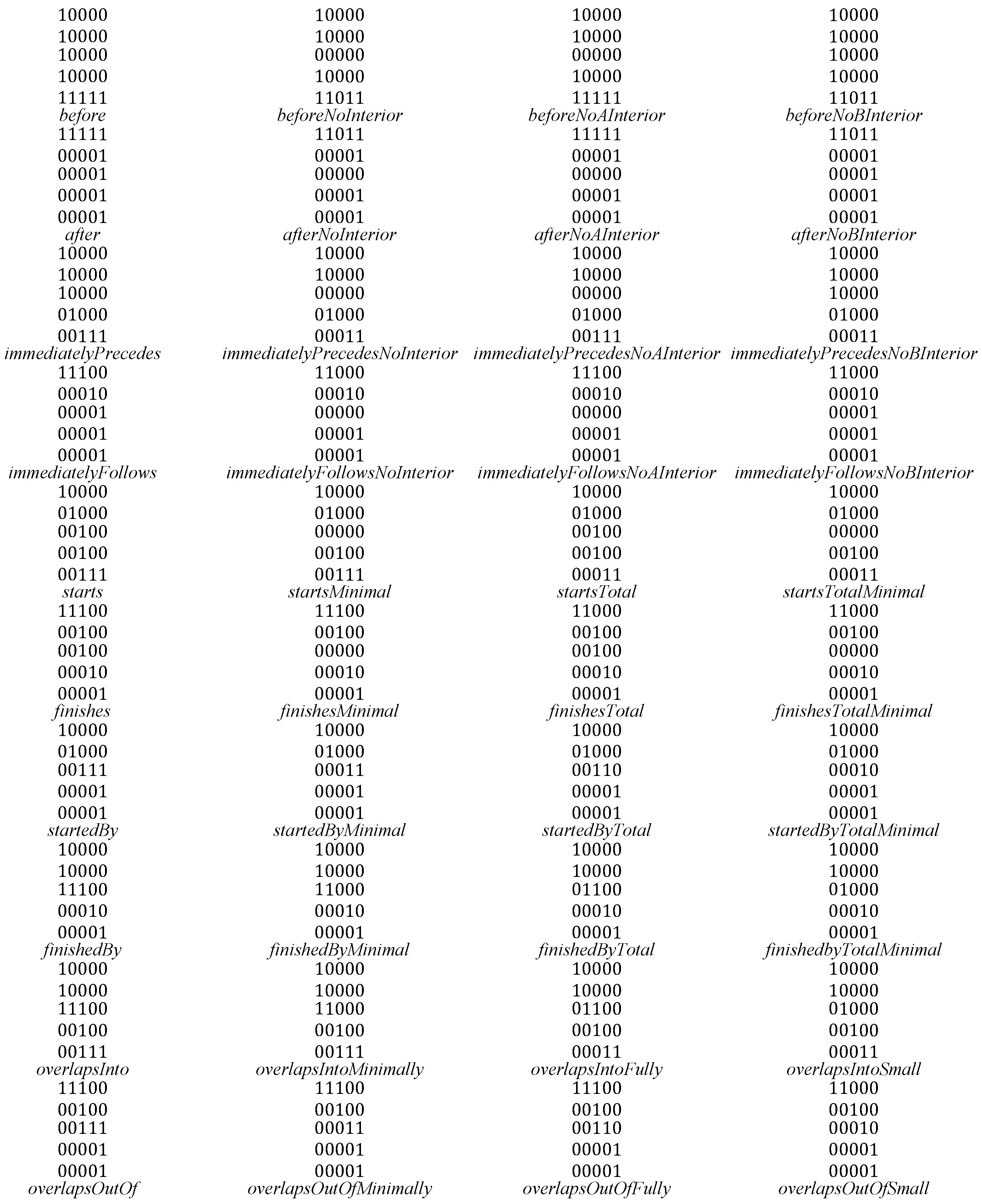Section 5 transforms these relations into their temporal counterparts through folding and extension into the 9+-intersection, bifurcating the exterior and boundary intersections. Finally, Section 6 discusses the work, shows application examples, and provides calls for future work in this area.

2. Foundational Mathematics for the Paper

The mathematics of qualitative topological relations in the 9-intersection family of models have their backbone in a hybridized version of point-set and algebraic topology [8,9]. In this section, we detail the foundations of point-set topology [32] that will loosely be translated conceptually into digital lines in ${\mathbb{Z}}^1$. Definitions 2–5 align with basic intuition about inside, outside, and edge, making them the most relevant starting point for this paper [2].

Definition 1 (Set).

Let A be a collection of points from within an embedding space. A is called a set.

Definition 2 (Interior).

Let A be a set of points within a topological space X. The interior of A, denoted $A^0$, is the largest open set from the topological space X contained within A.

Definition 3 (Exterior).

Let A be a set of points within a topological space X. The complement of the set A, denoted by $A^{-}$, represents the exterior of the set.

Definition 4 (Closure).

Let A be a set of points within a topological space X. The closure of set A, denoted  $\overline{A}$, is the smallest closed set from the topological space X, that contains A.

Definition 5 (Boundary).

Let A be a set of points within a topological space X. The boundary of the set A, denoted  $\partial A$, is the set $\overline{A}\backslash A^0$.

The interior, boundary, and exterior of an object form the vocabulary for the 9-intersection matrix [9]. The 9-intersection matrix (Equation (1)) considers the intersection between these topological components of two such objects A and B in a pairwise manner.

$$rel\left(A,B\right)=\begin{array}{ccc}{A}^0\cap B^0& A^0\cap \partial B& A^0\cap B^{-}\\ \partial A\cap B^0& \partial A\cap \partial B& \partial A\cap B^{-}\\ A^{-}\cap B^0& A^{-}\cap \partial B& A^{-}\cap B^{-}\end{array}$$

(1)

The structure and definition of the topological components in the 9-intersection family of models is dependent upon the topology induced upon the embedding space, making this family of formalisms extremely flexible for practical application in information systems. This allows practitioners to use formal topological approaches or to engineer topologically motivated conventions to better represent the desiderata of a system. This formalism was designed with simple objects in mind and gives binary detail (yes or no) about whether an intersection is empty or not. Simple objects in a naïve sense are those that have connected interiors, boundaries, and exteriors. Other types of embedding spaces and other types of objects create circumstances where an object may separate portions of the interior (or any other part) from one another. In situations such as this, an extension to the 9-intersection matrix called the 9+-intersection matrix [31] was developed. This has been used to describe simple objects [33], raster-based objects [22,34], and directed line segments [31] by deconstructing the topological components into regular prototypical simple objects. This technique has also been used to develop nomenclatures for scene recognition [35,36,37,38]. A different extension of this intersection technique is known as the dimensionally extended 9-intersection matrix [10], a common fixture in spatial reasoning applications. An example of the 9+-intersection for two objects, each with a disconnected boundary and exterior, is shown in Equation (2). While the 9+-intersection is capable of expressing far more complex objects, this specific representation will be leveraged in Section 5 of the paper as digital line segments have disconnected exterior components with semantic relevance (−< before and −> after) and two boundary points ($\partial$ < start and $\partial$ > end), each with semantic difference and more than likely disconnected in their own right. For the remainder of this paper, the partitions of the boundary and exterior of an object (where applicable) will follow the following naming conventions.

$$rel\left(A,B\right)=\begin{array}{cc}\begin{array}{ccc}{A}^{-<}\cap B^{-<}& A^{-<}\cap {\partial B}^{<}& A^{-<}\cap B^0\\ {\partial A}^{<}\cap B^{-<}& {\partial A}^{<}\cap {\partial B}^{<}& {\partial A}^{<}\cap B^0\\ A^0\cap B^{-<}& A^0\cap {\partial B}^{<}& A^0\cap B^0\end{array}& \begin{array}{cc}{A}^{-<}\cap {\partial B}^{>}& A^{-<}\cap B^{->}\\ {\partial A}^{<}\cap {\partial B}^{>}& {\partial A}^{<}\cap B^{->}\\ A^0\cap {\partial B}^{>}& A^0\cap B^{->}\end{array}\\ \begin{array}{ccc}{\partial A}^{>}\cap B^{-<}& {\partial A}^{>}\cap {\partial B}^{<}& {\partial A}^{>}\cap B^0\\ A^{->}\cap B^{-<}& A^{->}\cap {\partial B}^{<}& A^{->}\cap B^0\end{array}& \begin{array}{cc}{\partial A}^{>}\cap {\partial B}^{>}& {\partial A}^{>}\cap B^{->}\\ A^{->}\cap {\partial B}^{>}& A^{->}\cap B^{->}\end{array}\end{array}$$

(2)

In the case of a digital line in ${\mathbb{Z}}^1$, objects have disconnected exterior components and disconnected boundary components by default, all while maintaining a connected interior (if the interior exists at all). If the interior does not exist, then the two boundary points are connected, but in no circumstance may the exterior be connected. The boundary points, however, have a distinct characterization in that one of them can be thought of specifically as the starting point, while the other is the ending point when we consider concepts such as flow, routing, or time. This creates a 5 × 5 grid to explain topological relations within the 9+-intersection matrix that can be recombined into the 9-intersection as needed [34].

Three types of approaches are used to represent topological objects in not only continuous spaces but digital spaces as well. Digital spaces, however, provide a practical challenge: how does one define boundary? The most simplistic utilizes standard digital topology, resulting in pixels as the interior or exterior and the edge between the outermost pixels of the object and the exterior as the boundary [32,39]. This approach yields for regions in ${\mathbb{Z}}^2$ the same set of relations that exist in ${\mathbb{R}}^2$ [21] and would similarly do the same in linear embedding. The second approach is the digital Jordan curve [40]. Mirroring the philosophy of the point-set topology version of the Jordan curve theorem, the outermost pixels of an object are declared to be its boundary pixels; thus, every boundary pixel theoretically borders both interior pixels and exterior pixels (just as in continuous embeddings), while the interior pixels never border the exterior pixels and vice versa. This approach yields 16 relations in ${\mathbb{Z}}^2$ under the 9-intersection [20], and a further 3 additional relations when employing the 9+-intersection [31]. This approach also has the effect of making it possible that a line segment would not have an interior if it were sufficiently small compared with the resolution of the space, complicating the process of inventorying potential relations as will be seen in Section 4. The final method for representing these types of regions incorporates a margin approach [41]. The margin approach identifies rings on each side of the boundary to help alert if objects are near each other, the inner of which being the digital Jordan curve boundary. This approach adds the additional three relations in ${\mathbb{Z}}^2$ [20]. This type of approach has been used to extend beyond non-simple regions to simply connected regions (yielding 62 relations) [23] and has been extended to the digital sphere (yielding 29 relations) [24]. In this paper, we will utilize the digital Jordan curve, though it would be possible to include a margin approach to provide subtle distinctions between various digital Jordan curve relations with minimal modification (resulting in what are called touch relations, seen in Section 4). For a more rigorous formalization of the digital Jordan curve, please consult [40]. For the purposes of this manuscript, the intuitive definition of the immediate endpoints of the object representing the boundary, the interior being between those endpoints, and the exterior being beyond those endpoints will suffice. Employing a margin approach would lead to a more complicated 9+-intersection matrix. A comparative figure to show the three types of boundary approaches is shown in Figure 2.

For the remainder of this paper, we will consider the class of intervals represented in ${\mathbb{Z}}^1$ (Definition 7). Each interval can be seen as simply a line segment in the space (pursued in Section 4) but can also be seen as a directed line segment with a starting point and an ending point (pursued in Section 5). Definitions 6 and 7 set the stage for the discussion of these types of objects in Section 4 and Section 5.

Definition 6 (Connected).

Let P be a collection of pixels in a discrete space. P is connected if there exists an exhaustive sequence of pixels p₁, p₂, … p_n such that p_i neighbors both p_i−1 and p_i+1.

Definition 7 (Interval object).

Let I be a finite group of connected pixels in ${\mathbb{Z}}^1$ consisting of at least two pixels. I is defined as an interval object.

With the definition of connected interval objects constructed, the paper can move forward to constructing constraints that must exist on the 9-intersection relation between two such objects.

3. Line–Line Relations in a Continuous Linear Embedding Space

The seminal research motivating line–line relations in linear embeddings is well established and has been the subject of decades of further research. While this paper is not concerned specifically with continuous linear embedding spaces such as ${\mathbb{R}}^1$, the basic building blocks of the presentation of the results of this paper are most easily conveyed with these relations in mind as, ultimately, the goal of information systems is to produce responses that are in cognitive alignment with their users’ cognitive states.

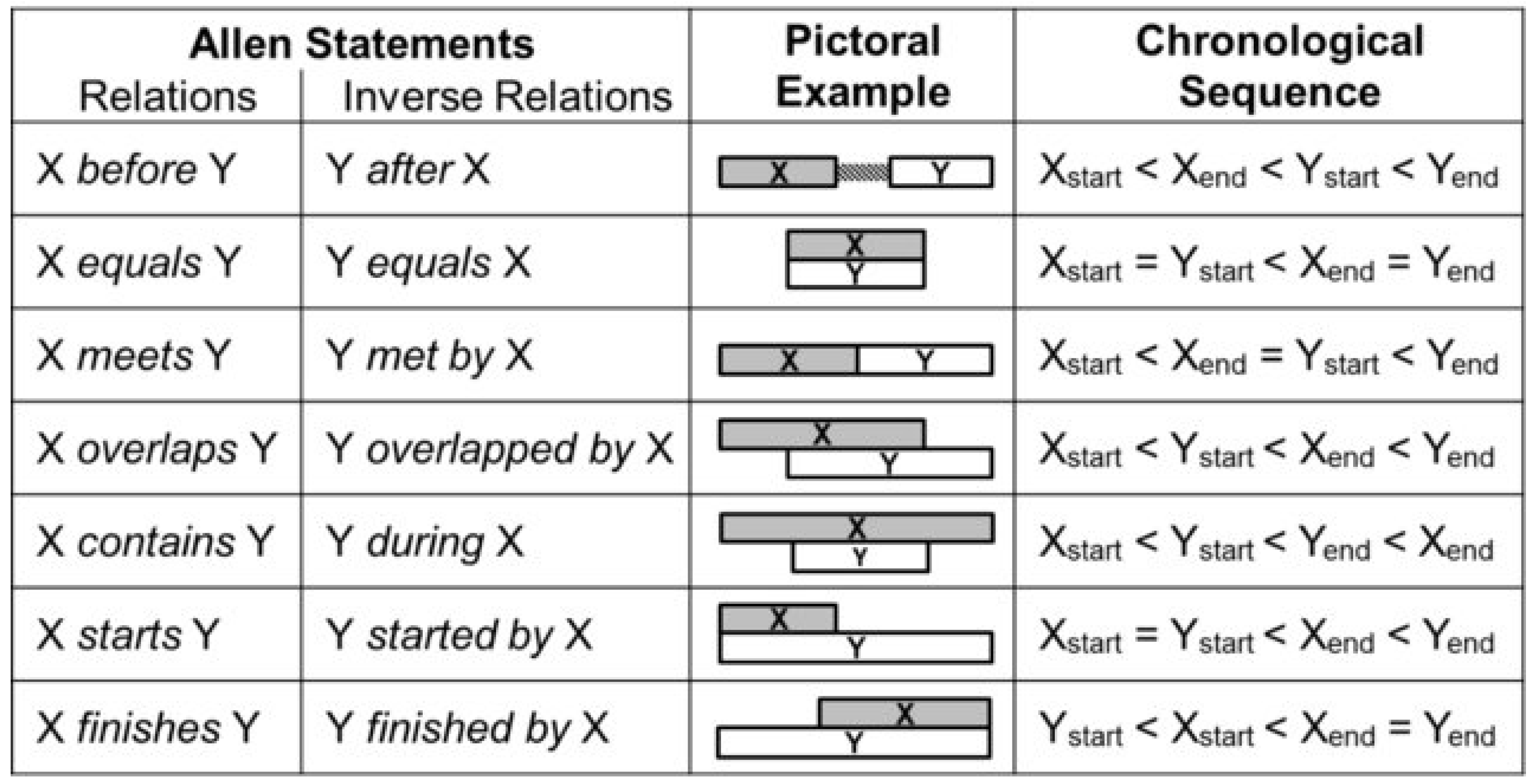
Allen’s interval algebra [7] considers the relationships between the starting and ending points of two objects. The sequence of the points in question defines the relation between the intervals. Allen identified 13 plausible sequences for the four points (Figure 3), collapsible into seven groups.

Using the 9-intersection, intervals in ${\mathbb{R}}^1$ can also be studied, removing the ordering principle from Allen’s interval algebra. If we consider the pictorial representations in Figure 3, we can assess definitively the 9-intersection matrices associated with them. These are shown in Figure 4. Interestingly, contains and during form two separate 9-intersection relations.

The folding of the Allen intervals reflects the notion that the order in which the objects occur is irrelevant in the spatial domain in that specific context. If the order were consequential, the 9+-intersection would be used to capture it by distinguishing the start/endpoints and the before and after exteriors.

With knowledge of the state of the art in continuous space, we can now move on to developing similar relations in discretized spaces. Going forward in the manuscript, we will use these simpler relations to group the more numerous discretized relations, showing the fundamental relationship between Allen’s interval algebra and continuous relations to their discretized counterparts.

4. Line–Line Relations in a Discretized Linear Embedding Space

To determine the types of relations available within ${\mathbb{Z}}^1$, we have to consider different types of objects that can form digital intervals. This is methodologically a deviation from continuous spaces where the embedding space is dense, making the concern irrelevant in that domain. Because a discretized space is not dense, it becomes possible for boundaries of objects to exhaust topological portions (i.e., boundary, interior, and exterior) or for closures of objects (boundary + interior) to do the same. This represents a critical difference between ${\mathbb{Z}}^1$ and ${\mathbb{R}}^1$ that has the effect of ballooning possible relations.

Digital intervals can have interior pixels or not when considering the digital Jordan curve. The number of interior pixels (0, 1, 2, or 3+) can have an impact on the types of digital relations available because the various sizes convey whether a boundary or the closure of an object can exhaust the interior pixels of the other. An interior with zero pixels creates a line consisting entirely of a boundary; an interior with one pixel allows for a single boundary component to exhaust the interior; an interior with two pixels can be exhausted by an object with no interior pixels; an interior with 3+ pixels would facilitate the capability of containing a digital line with an interior, possibly exhaustive. We will thus break our consideration down into different groups of objects to extract the relevant qualitative digital relations in the space using a constraint sieve. The constraint sieve will systematically eliminate possibilities. At the conclusion of the constraint sieve, the remaining relations should be realizable between two interval objects as described in Definition 7 and, as a matter of presentation, will be shown in figures throughout the analysis.

A set of basic constraints exist between an object’s topological components and between the interplay of objects’ topological components within a relation by virtue of the structure of interval objects. Because the 9-intersection and the 9+-intersection leverage knowledge of the intersection of topological components of the two objects involved, each constraint can be expressed somehow through elements of these symbolic representations. As such, the discussion begins with constraints that exist independent of an object’s interior cardinality. These constraints largely follow constraint logic used in discretized reasoning papers with respect to region relations [20,23,24,34], amended appropriately to account for the separated exterior and boundary of a digital line unique to linear embedding spaces.

• Constraint 1: An interval object I must have an exterior.

• Rationale: ${\mathbb{Z}}^1$ is a countably infinite space. Since I is finite by construction (cardinality of interior + 2), there must exist at least one pixel z that does not belong to that object.

C1 passes down to the 9-intersection that at least one member of the $A^{-}$ row must be non-empty and that at least one member of the $B^{-}$ column must also be non-empty.

• Constraint 2: Two interval objects I and J in a space must have at least one pixel in common between their exteriors.

• Rationale: Consider $I\cup J$. Since the cardinality of both I and J is finite, then their union has cardinality of at most |I| + |J|, which is still finite. By C1, there exists such a pixel exterior to the union, and therefore exterior to both. Conveniently, C2 immediately refines C1 in ${\mathbb{Z}}^1$; however, C2 would not be enforced in ${\mathbb{T}}^1$ as two objects could together exhaust the space, a result similar to continuous parallels ${\mathbb{R}}^1$ and ${\mathbb{S}}^1$ [17], producing relations such as attach, embrace, and entwined.

C2 passes down to the 9-intersection that no matter what, two objects A and B are under consideration in ${\mathbb{Z}}^1$,

$$A^{-}\cap B^{-}=\neg \mathrm{\varnothing }$$

(3)

• Constraint 3: An interval object I has exactly two boundary pixels.

• Rationale: The definition of a boundary, utilizing the digital Jordan curve, dictates that boundary pixels are those pixels which neighbor exterior pixels. Since I has at least two pixels, two of them (namely the outermost two) must touch $I^{-}$. In this case, each boundary pixel touches a different connected component of $I^{-}$.

C3 passes down to the 9-intersection that the $\partial A$ row must have exactly one or two non-empty intersections and that the $\partial B$ column must have exactly one or two non-empty intersections, namely

$$0<\left|\partial A\cap \mathrm{*}\right|\le 2$$

(4)

$$0<\left|*\cap \partial B\right|\le 2$$

(5)

These could produce 1 only if both boundary pixels occupy the same topological component of their relation partner. In all other cases, these will produce 2.

• Constraint 4: If the boundaries of interval objects I and J are identical, then their interiors and exteriors must be identical as well.

• Rationale: Constraint 4 depends upon the connectivity of the interior and the finite cardinality of the interior. Since ${\mathbb{Z}}^1\backslash \partial I$ has separated components (and only one of them has a finite cardinality), the one with a finite cardinality is the interior, and the union of the other two is the exterior, as the boundary must surround the interior. Similarly to C2, C4 would not be enforced in ${\mathbb{T}}^1$ as the exterior would also be finite.

C4 passes down the following to the 9-intersection:

$$\begin{array}{c}(\partial A\cap B^0=\mathrm{\varnothing }\wedge \partial A\cap \partial B=\neg \mathrm{\varnothing }\wedge \partial A\cap B^{-}=\mathrm{\varnothing })\therefore (A^0\cap \partial B=\mathrm{\varnothing }\wedge A^0\cap B^{-}\\ =\mathrm{\varnothing })\wedge (A^{-}\cap B^0=\mathrm{\varnothing }\wedge A^{-}\cap \partial B=\mathrm{\varnothing }\wedge A^{-}\cap B^{-}=\neg \mathrm{\varnothing })\end{array}$$

(6)

$$\begin{array}{c}(A^0\cap \partial B=\mathrm{\varnothing }\wedge \partial A\cap \partial B=\neg \mathrm{\varnothing }\wedge A^{-}\cap \partial B=\mathrm{\varnothing })\therefore (\partial A\cap B^0=\mathrm{\varnothing }\wedge A^{-}\cap B^0\\ =\mathrm{\varnothing })\wedge (A^0\cap B^{-}=\mathrm{\varnothing }\wedge \partial A\cap B^{-}=\mathrm{\varnothing }\wedge A^{-}\cap B^{-}=\neg \mathrm{\varnothing })\end{array}$$

(7)

Depending on whether objects have interiors or not, the missing intersection ($A^0\cap B^0$) will be either empty (no interior) or non-empty (interior exists).

• Constraint 5: If both of the boundaries of interval object I are in the interior of another interval object J, then$I^0\cap \partial J=\varnothing \wedge I^0\cap J^{-}=\varnothing$.

• Rationale: Because the boundary pixels surround the connected interior pixels of I and the interior of J is connected by definition, both $\partial J$ and $J^{-}$ cannot exist in that space.

C5 passes down the following to the 9-intersection:

$$(\partial A\cap B^0=\neg \mathrm{\varnothing }\wedge \partial A\cap \partial B=\mathrm{\varnothing }\wedge \partial A\cap B^{-}=\mathrm{\varnothing })\therefore (A^0\cap \partial B=\mathrm{\varnothing }\wedge A^0\cap B^{-}=\mathrm{\varnothing })$$

(8)

$$(A^0\cap \partial B=\neg \mathrm{\varnothing }\wedge \partial A\cap \partial B=\mathrm{\varnothing }\wedge A^{-}\cap \partial B=\mathrm{\varnothing })\therefore (\partial A\cap B^0=\mathrm{\varnothing }\wedge A^{-}\cap B^0=\mathrm{\varnothing })$$

(9)

Depending on whether or not objects have interiors, the missing intersection ($A^0\cap B^0$) will be either empty (no interior) or non-empty (interior exists).

Such a constraint can be violated in ${\mathbb{T}}^1$, just as the similar condition can be violated in ${\mathbb{S}}^1$ when considering continuous line relations [17].

C1–C5 provide restrictions that exist independent of whether or not the interior of either or both objects exists. To continue forward, we must identify existing constraints that are unique to objects that must have interiors.

• Constraint 6: If the interior or exterior of an interval object I (I* is used to denote the topological component in question) intersects both the interior and exterior of an interval object J, then $I^{*}\cap \partial J=\neg \varnothing$.

• Rationale: The boundary of an object divides the interior from the exterior. For the interior, this is guaranteed because the interior of I must be connected. For the exterior, this is a bit more work. $I^{-}$ is disconnected within ${\mathbb{Z}}^1$. To demonstrate this, it must be shown that the interior intersection and the exterior intersection can occur on the same side of I. Consider an exposed interior pixel of J. Without loss of generality, assume that the exposed interior pixel is to the left of I’s boundary. This pixel’s left neighbor is either in J’s interior or boundary. If it is in J’s interior, continue left until the boundary is reached, satisfying the constraint. To violate this constraint would require that I had a separated interior, which, by construction, is a contradiction of the definition of an interval object (Definition 7).

C6 passes down the following to the 9-intersection:

$$A^{-}\cap B^0=\neg \mathrm{\varnothing }\wedge A^{-}\cap B^{-}=\neg \mathrm{\varnothing }\therefore A^{-}\cap \partial B=\neg \mathrm{\varnothing }$$

(10)

$$A^0\cap B^0=\neg \mathrm{\varnothing }\wedge A^0\cap B^{-}=\neg \mathrm{\varnothing }\therefore A^0\cap \partial B=\neg \mathrm{\varnothing }$$

(11)

$$A^0\cap B^0=\neg \mathrm{\varnothing }\wedge A^{-}\cap B^0=\neg \mathrm{\varnothing }\therefore \partial A\cap B^0=\neg \mathrm{\varnothing }$$

(12)

$$A^0\cap B^{-}=\neg \mathrm{\varnothing }\wedge A^{-}\cap B^{-}=\neg \mathrm{\varnothing }\therefore \partial A\cap B^{-}=\neg \mathrm{\varnothing }$$

(13)

• Constraint 7: If the two boundaries of interval object I are within the interior of interval object J and the exterior of interval object J, respectively, then the two boundaries of J must be within the interior and exterior of object I.

• Rationale: By construction, the interior and exterior pixels of J must be separated by at least one pixel. Since the interior of object I sits between the two boundary pixels of I, it must include the boundary point of J between these two pixels. Since the interior must remain connected, all pixels between that boundary point and I’s interior boundary pixel are interior of J. Consider the next pixel to the left (or right, if beyond) of I’s interior boundary pixel. That pixel is either the interior of J or boundary of J. Continue until reaching the boundary of J as in Constraint 6, achieving the result.

C7 passes the following to the 9-intersection matrix:

$$(\partial A\cap B^0=\neg \mathrm{\varnothing }\wedge \partial A\cap B^{-}=\neg \mathrm{\varnothing })\leftrightarrow (A^0\cap \partial B=\neg \mathrm{\varnothing }\wedge A^{-}\cap \partial B=\neg \mathrm{\varnothing })$$

(14)

• Constraint 8: If both interval objects I and J have a boundary pixel in each other’s interior and their exteriors share a common intersection, then the boundaries of I and J cannot intersect.

• Rationale: Similarly to that in C7, a pixel declared as a boundary inside the interior of another object has neighbors that are either the interior or boundary. If not the boundary, traversing further in that direction will encounter the boundary that is in the exterior. Therefore, finding the interior boundary of one results in finding the exterior boundary of the other, traversing opposite of one’s own interior. When applied to both objects, no construction can produce a boundary–boundary intersection. Given that C2 asserts that there must be a common exterior, this is enough to demonstrate the constraint.

C8 passes the following to the 9-intersection:

$$\left(\partial A\cap B^0=\neg \mathrm{\varnothing }\wedge A^0\cap \partial B=\neg \mathrm{\varnothing }\right)\therefore \partial A\cap \partial B=\mathrm{\varnothing }$$

(15)

• Constraint 9: If both interval objects I and J have a boundary pixel in each other’s exterior and their interiors share a common intersection, then the boundaries of I and J cannot intersect.

• Rationale: Constraint 9 is the dual of C8 [43].

C9 passes the following to the 9-intersection:

$$\left(\partial A\cap B^{-}=\neg \mathrm{\varnothing }\wedge A^{-}\cap \partial B=\neg \mathrm{\varnothing }\wedge A^0\cap B^0=\neg \mathrm{\varnothing }\right)\therefore \partial A\cap \partial B=\mathrm{\varnothing }$$

(16)

• Constraint 10: If both boundaries of an interval object I are within the exterior of object J, then either the entire interior of I is in the exterior of object J, the interior of I is the closure of J, or the interior of I will cross all three components.

• Rationale: These three possibilities stem from the placement of the boundary of I relative to J. If I’s boundary pixel is not adjacent to a boundary pixel of J, then an interior pixel of I intersects J’s exterior. If the other boundary pixel of I occurs sequentially before encountering J’s boundary, then we have the first condition. If I’s interior encounters J’s boundary, then it must continue until it reaches and passes J’s other boundary to retain both boundary pixels of I in J’s exterior. This is the third condition. The second condition is attained by placing I’s boundary directly adjacent to J’s boundary on both ends of J. The interior then intersects only J’s interior and boundary.

C10 passes the following constraints to the 9-intersection matrix:

$$\begin{array}{cc}(\partial A\cap B^0=\mathrm{\varnothing }\wedge & \partial A\cap \partial B=\mathrm{\varnothing }\wedge \partial A\cap B^{-}=\neg \mathrm{\varnothing })\therefore (A^0\cap B^0=\mathrm{\varnothing }\wedge A^0\cap \partial B\hfill \\ & =\mathrm{\varnothing }\wedge A^0\cap B^{-}=\neg \mathrm{\varnothing })\vee (A^0\cap B^0=\neg \mathrm{\varnothing }\wedge A^0\cap \partial B\hfill \\ & =\neg \mathrm{\varnothing }\wedge A^0\cap B^{-}=\neg \mathrm{\varnothing })\vee (A^0\cap B^0=\neg \mathrm{\varnothing }\wedge A^0\cap \partial B\hfill \\ & =\neg \mathrm{\varnothing }\wedge A^0\cap B^{-}=\mathrm{\varnothing })\hfill \end{array}$$

(17)

$$\begin{array}{cc}(A^0\cap \partial B=\mathrm{\varnothing }\wedge & \partial A\cap \partial B=\mathrm{\varnothing }\wedge A^{-}\cap \partial B=\neg \mathrm{\varnothing })\therefore (A^0\cap B^0=\mathrm{\varnothing }\wedge \partial A\cap B^0\hfill \\ & =\mathrm{\varnothing }\wedge A^{-}\cap B^0=\neg \mathrm{\varnothing })\vee (A^0\cap B^0=\neg \mathrm{\varnothing }\wedge \partial A\cap B^0\hfill \\ & =\neg \mathrm{\varnothing }\wedge A^{-}\cap B^0=\neg \mathrm{\varnothing })\vee (A^0\cap B^0=\neg \mathrm{\varnothing }\wedge \partial A\cap B^0\hfill \\ & =\neg \mathrm{\varnothing }\wedge A^{-}\cap B^0=\mathrm{\varnothing })\hfill \end{array}$$

(18)

The final constraint dictates the conditions for the sieve that guarantee whether the objects have an interior or not. For various sets of relations, these two constraints can be turned on or off where appropriate.

• Constraint 11: An interval object A must have an interior.

  $$A^0\cap B^0=\neg \varnothing \vee A^0\cap \partial B=\neg \varnothing \vee A^0\cap B^{-}=\neg \varnothing$$

  (19)

  $$A^0\cap B^0=\neg \varnothing \vee \partial A\cap B^0=\neg \varnothing \vee A^{-}\cap B^0=\neg \varnothing$$

  (20)

4.1. Two Objects with Interiors (C11 Active upon Both Intervals)

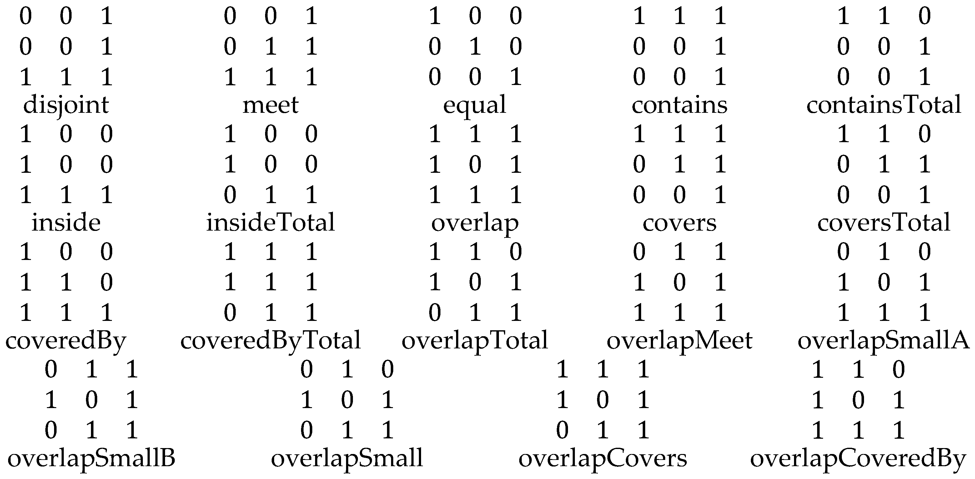
Applying these constraints to the class of 9-intersection relations produces 19 viable topological relations with distinct 9-intersection signatures when the objects both have an interior. That is three more than in the simple region–region relations in ${\mathbb{Z}}^2$ [20]. The resulting relations are shown in Figure 5. Notably, the line–line relations in ${\mathbb{R}}^1$ have the exact same set of relations as the corresponding region–region relations in ${\mathbb{R}}^2$.

4.2. Two Objects with No Interiors (C11 Reversed to Forbid Interior)

The relations between two objects with no interiors are much simpler to construct conceptually but can also be constructed by substituting constraint C11 with a constraint that no interior intersection can exist. On an intuitive level, this set can be thought of in three distinct forms: (1) the two boundaries are identical, implying that the two exteriors are equal; (2) the two boundaries are entirely distinct, implying a version of disjoint; and (3) one boundary is in common, while the others are different. This is the equivalent of meet or overlap. The three symbols for this are shown in Figure 6.

4.3. One Object with an Interior, One Object Without an Interior

While this result could be considered using a constraint sieve, this case is just as easily accomplished with a visual inspection. We must consider three distinct cases: (1) the object with an interior has only one interior pixel, (2) the object with an interior has exactly two interior pixels, and (3) the object with an interior has three or more pixels. Each class leads to similar relations, but in some cases, there are distinct relations that occur. These classes can alternatively be addressed by substituting C11 for one of the two objects with its juxtaposition, but not the other.

4.3.1. Common Core

The common core relations between these three cases are ones where the two pixels of the interior-less object do not encounter the interior of the other object. There are four such cases: disjoint (and its converse) and meet (and its converse), as shown in Figure 7.

4.3.2. One-Pixel Interior

The relations with the one-pixel interior that are added are all versions of coversTotal and coveredByTotal. The object that has the one-pixel interior will always subsume the other. These relations in this form are not shared by the two-pixel interior or above, yet there are distinct covers and coveredBy relations that appear in those sets. These relations are shown in Figure 8.

4.3.3. Two-Pixel Interior

The relations with the two-pixel interior that are added are versions of covers, coveredBy, insideTotal, and containsTotal. These relations are shown in Figure 9.

4.3.4. 3+ Pixel Interior

The relations with more than two pixels in their interior in this group of object relations add the potential for a proper contains or inside. These relations are shown in Figure 10.

When combining all of these sets, we determine 34 distinct 9-intersection symbols between two objects A and B in ${\mathbb{Z}}^1$.

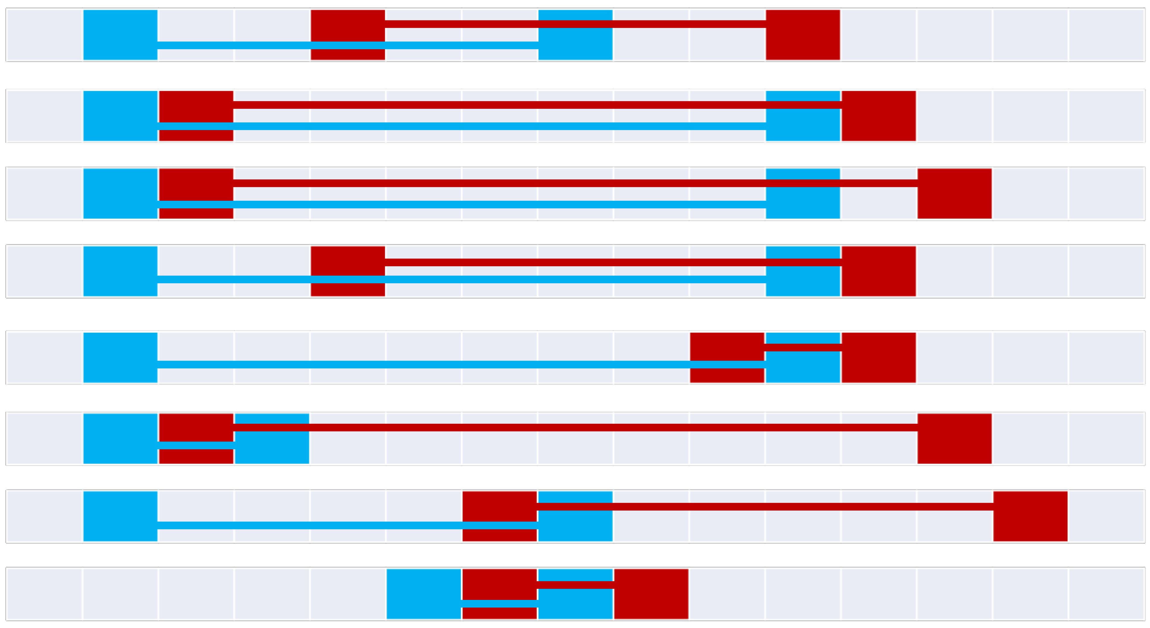
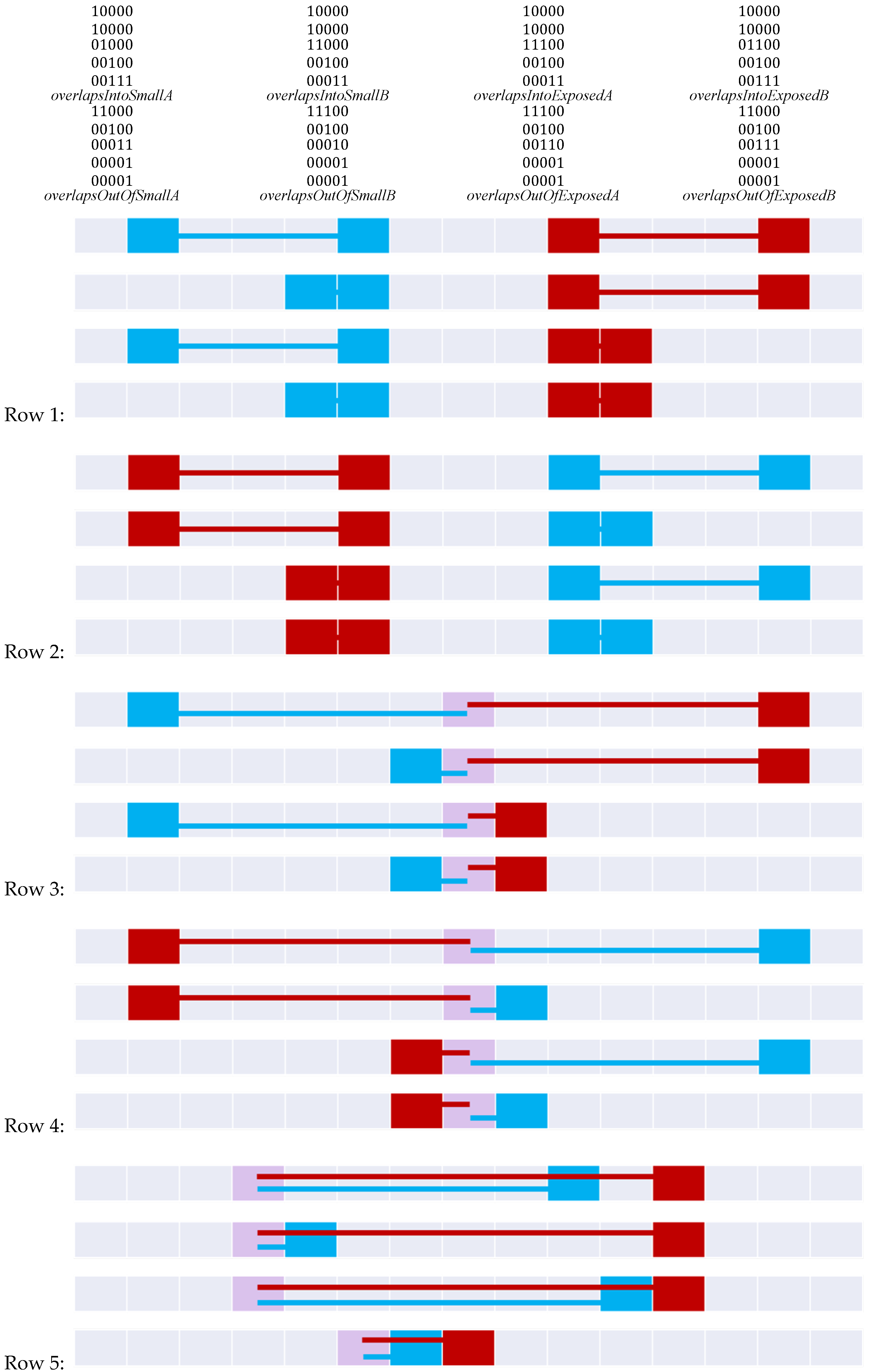
4.4. Visualizing the Set

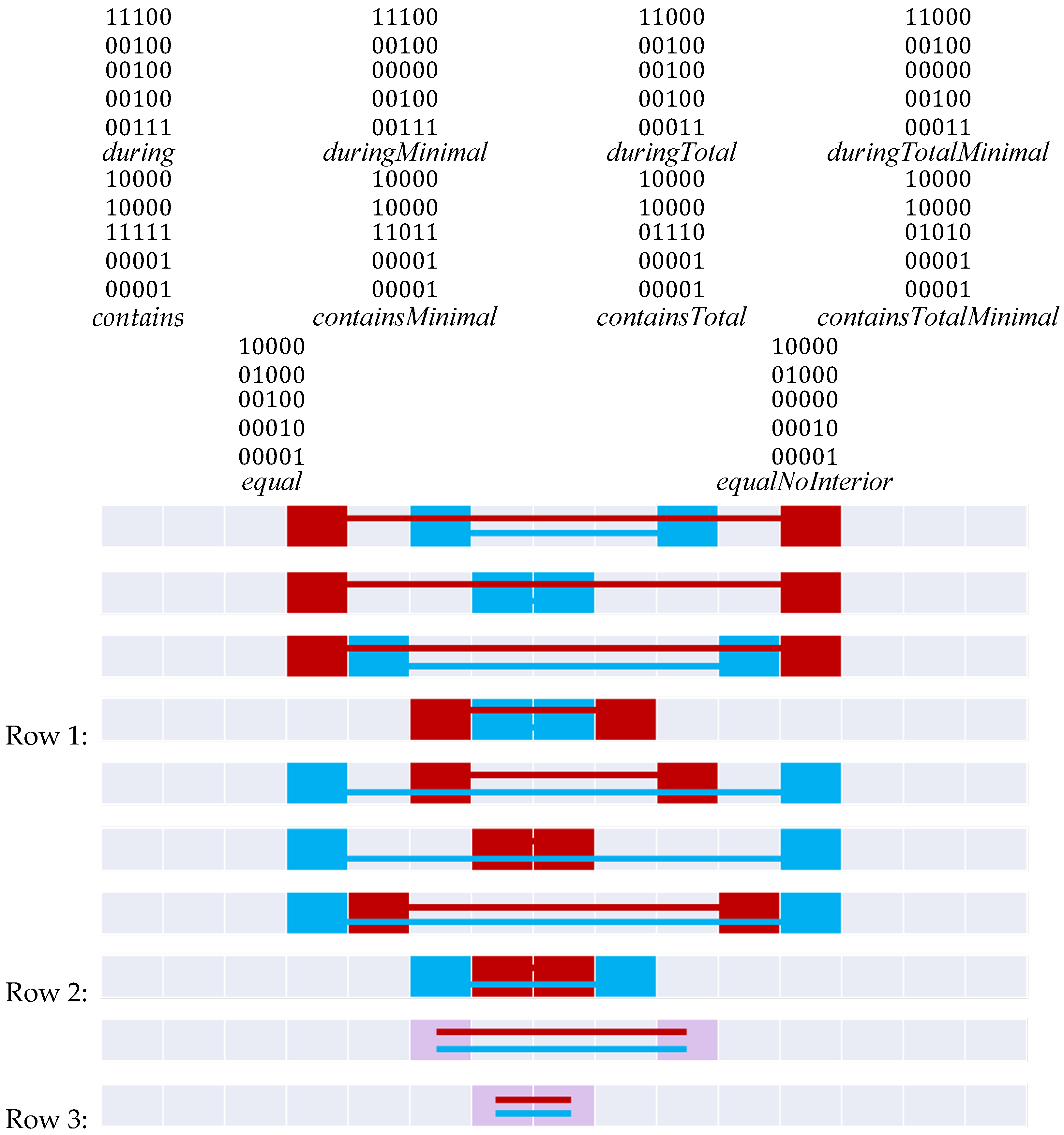
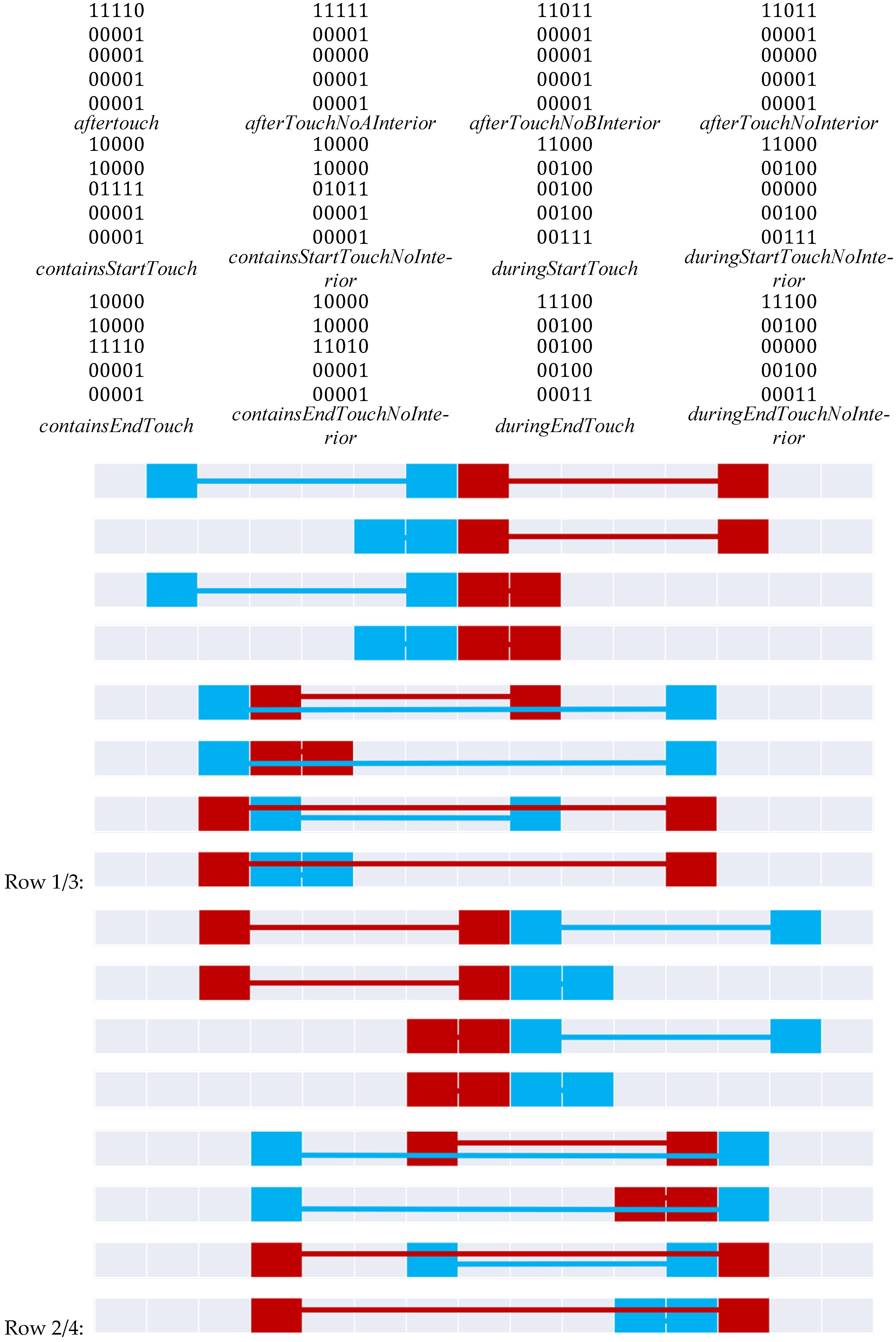
Figure 11, Figure 12, Figure 13, Figure 14, Figure 15, Figure 16, Figure 17 and Figure 18 demonstrate the various relations as an entire set, organized by their parent line–line relation in ${\mathbb{R}}^1$ from Figure 4. In all cases, the blue object is line A, and the red object is line B. If two boundaries are shared, the boundary point is purple. If the lines encounter common pixels (including boundaries), the two connectors are offset to convey the path (A on bottom, B on top).

This is a good first start, but it is not complete. While most scenarios are accounted for by this simple symmetric exercise, the touch relationships [20,24,34] that are not distinguishable by the 9-intersection for spatial relations disjoint, inside, and contains are not.

The discrete region–region relations in ${\mathbb{Z}}^2$ also rely on boundary adjacency (a concept that cannot be modeled directly with the 9-intersection) to produce the relations disjointTouch, insideTouch, and containsTouch. Using a similar philosophy, each version of disjoint, pure inside, and pure contains can be bifurcated as in Figure 19. Figure 19 displays the type of relation that is bifurcated from the prototype relations from Figure 11, Figure 13 and Figure 14.

All told, when considering this bifurcation, 42 distinct relations exist between non-ordered lines in ${\mathbb{Z}}^1$, shown in Figure 11, Figure 12, Figure 13, Figure 14, Figure 15, Figure 16, Figure 17, Figure 18 and Figure 19. If looking only for distinct 9-intersection matrices, there are 34 relations, shown in Figure 11, Figure 12, Figure 13, Figure 14, Figure 15, Figure 16, Figure 17 and Figure 18.

5. Digital Temporal Relations

When ${\mathbb{Z}}^1$ is treated as time, this induces an ordering which bifurcates certain relations into copies, depending on which boundary is shared or which exterior is intersected (e.g., the coveredBy relations into starts and finishes). Temporal relations make use of the 9+-intersection to be able to distinguish which boundary and which exterior they interact with specifically. In a sense, we can accomplish the same concept by examining which types of relations can be formed in two directions, versus relations which are inherently symmetric. The discretized temporal relations will be presented in the 9+-intersection in the following arrangement:

$$\begin{array}{cc}\begin{array}{ccc}{A}^{-<}\cap B^{-<}& A^{-<}\cap {\partial B}^{<}& A^{-<}\cap B^0\\ {\partial A}^{<}\cap B^{-<}& {\partial A}^{<}\cap {\partial B}^{<}& {\partial A}^{<}\cap B^0\\ A^0\cap B^{-<}& A^0\cap {\partial B}^{<}& A^0\cap B^0\end{array}& \begin{array}{cc}{A}^{-<}\cap {\partial B}^{>}& A^{-<}\cap B^{->}\\ {\partial A}^{<}\cap {\partial B}^{>}& {\partial A}^{<}\cap B^{->}\\ A^0\cap {\partial B}^{>}& A^0\cap B^{->}\end{array}\\ \begin{array}{ccc}{\partial A}^{>}\cap B^{-<}& {\partial A}^{>}\cap {\partial B}^{<}& {\partial A}^{>}\cap B^0\\ A^{->}\cap B^{-<}& A^{->}\cap {\partial B}^{<}& A^{->}\cap B^0\end{array}& \begin{array}{cc}{\partial A}^{>}\cap {\partial B}^{>}& {\partial A}^{>}\cap B^{->}\\ A^{->}\cap {\partial B}^{>}& A^{->}\cap B^{->}\end{array}\end{array}$$

(21)

5.1. Bi-Directional Relations from Figure 11, Figure 12, Figure 15, Figure 16 and Figure 18

Figure 20 constructs the 9+-intersection [31] for each of the bifurcated asymmetric relations found in Figure 11, Figure 12, Figure 15, Figure 16 and Figure 18. The rows of the figure are paired, namely each odd row considers A interacting with B’s before exterior and its start, while the even rows show A’s interaction with B’s after exterior and its end where applicable. Visible representations are shown beneath the table, representing horizontal flips of the corresponding Figure 11, Figure 12, Figure 15, Figure 16 and Figure 18. This transformation is made possible by recognizing that there are two distinct versions of the ordering relations that govern these relations from Allen’s interval algebra [7], as shown in Figure 3. The name of each relation is derived from Allen’s interval algebra relation that corresponds semantically to the relation [7].

5.2. Symmetric Relations (10), Found in Figure 13, Figure 14 and Figure 17

The symmetric relations from Figure 13, Figure 14 and Figure 17 by their nature are the same if the corresponding figures are flipped horizontally. As such, no new matrices are created. Figure 21 shows the 9+-intersection matrices for these relations and repeats the images from Figure 13, Figure 14 and Figure 17.

5.3. Touch Relations (8)

When boundaries become adjacent with the 9+-intersection, interior–exterior intersections are removed. As such, we need to consider the eight relations between objects as shown in Figure 22, producing 16 more temporal relations.

This presents a total of 74 distinct 9+-intersection matrices to represent temporal intervals in ${\mathbb{Z}}^1$. These relations will exchange the start and endpoints of object A as well as the before and after exteriors associated with them. This directly explains the inflation of the set of relations from 34 to 74. The naming convention used in the relations provides a direct comparison with Allen’s interval algebra [7], a direct bifurcation of the 9-intersection relations in the non-symmetric cases.

6. Discussion

In this paper, the relations existing between two continuous sets in ${\mathbb{Z}}^1$ were explored, yielding 34 specific digital Jordan curve relations and 42 relations when adding appropriate adjacency information. These sets of relations have core similarities with each other as different objects shift and change size and are all generalizable to similar relations in the set of digital Jordan curve relations in ${\mathbb{Z}}^2$ [20]. As the boundaries are disconnected in these types of objects, different types of relations become possible to sustain that are not sustainable in other sets of region–region relations.

These relations were then bifurcated to form corresponding temporal relations, yielding 74 distinct digital Jordan curve relations in an ordered state when considering appropriate touch relations. Unlike with the pure 9-intersection, the 9+-intersection does change when the boundaries of two objects become adjacent. This occurs because an intersection is being deleted as the boundaries approach one another to the point of adjacency. These 74 relations become the building blocks for expressing more complex queries in spatio-temporal stacks. This concept recognizes the difference between a pure discrete cube embedding and the corresponding spatio-temporal stack: the vertical dimension is not the same semantically as the horizontal planar ones are, and thus that dimension must be treated separately rather than pursuing a digital cube relation.

Digital relations in ${\mathbb{Z}}^1$ lead to important unresolved problems in spatio-temporal information science. Most notably, digital relations between lines in ${\mathbb{Z}}^2$ have been elusive but represent the missing link in digital spatial reasoning. This paper surrounds that problem with three specific sets of relations that should provide meaningful insights into the process of deriving relationships in that embedding. The biggest challenge to that task is the sequencing of a path. Conceptually speaking, the task of deriving relationships between the pixels should be rather straightforward. This problem is important to solve as it recognizes the importance of leveraging both vectorized and discretized data in applications such as Geo-AI [13,27]. To meet the demands of variability in the format of datasets, we need to complete the discretized versions of every continuous space relation set we have in the qualitative spatial reasoning community. This paper fills two of those gaps.

The contributions of this manuscript come in two separate cases which need to be implemented into modern GIS.

The first instance is in the purely geographic case. Consider any spatial object which is conceptualized in a linear format under cartographic generalization (such as a river, road, or municipal boundary). The 34/42 relations identified in this paper serve as the vocabulary to express relations of interest within that discretized linear embedding space. For example, imagine a transportation engineer searching for sectors of traffic congestion and their relation to areas of construction. We might suspect that the relation between these two phenomena might come from the family of covers relations, suggesting that the road construction backs up the queue of traffic up to the construction zone and through to the end of the construction zone. A relation such as one from the disjoint family of relations might suggest the presence of an accident on the roadway, an entirely different source of congestion altogether. Because road networks are ordered (i.e., traffic flows in a direction), we can consider the 74 relations identified in this work to also be of distinct relevance. We would expect the traffic congestion to end with the road construction, but if there were an accident somewhere on the highway, the distinction between before and after becomes far more relevant to users, be they motorists or traffic analysts.

The second instance of applicability comes from within the spatio-temporal stack architecture. While modern GIS is equipped with tools to determine topological relations between objects in a spatial layer within a spatio-temporal stack [25,34], the modern GIS is not currently equipped with the ability to interpret relationships across layers of the spatio-temporal stack. The prototypical example of such a query would be to find instances of a topological relation x during the coverage of the spatio-temporal stack. Such a query is intuitively fulfilled simply by finding the topological relation x in any one of the layers of the stack. A different query would be to find instances of topological relation x that start other events found in the spatio-temporal stack. Those events may have a duration or not, projecting information about the event onto the temporal axis of the spatio-temporal stack. This instance is the fundamental breakthrough necessary to realize a qualitative spatio-temporal information system on the foundation of a spatio-temporal stack, as this paper provides the computational temporal prepositions that have been missing in the extant literature.

Relations do not exist necessarily in a vacuum, and this is particularly true for linear or planar spaces. These spaces in our natural world are often considered in cyclic versions of the same space. To fully realize the potential of spatial and temporal information, it is important to generalize from linear spaces to cyclic spaces. Such adaptations have journeyed from Allen’s interval algebra to the cycle algebra [7,17], from the RCC-8 relations to the RCC-11 relations [11,19], from the point-set topological relations to the spherical topological relations [9,18], and from the raster relations in ${\mathbb{Z}}^2$ to the raster relations in ${\mathbb{T}}^2$ [20,24]. This set of relations can be transformed using similar processes, completing the set of linear embeddings.

The other important step to take from this starting point is to consider the alphabet of spatio-temporal queries. Research has focused on spatial queries and temporal queries, but the queries that engage both together are fewer in number. Jiang et al. [44] studied the notion of topological changes in objects. While this is an important step, it does not solve issues that involve the sequence of binary relationships more related to conceptual neighborhood graphs [45,46]. That innovation will unlock many doors in spatial informatics in numerous application spaces, most notably as complex spatial phenomena related to species migration and shifting climates are knocking at our doors.

While this research develops an alphabet for spatial and spatio-temporal relations in a digital linear embedding space, it is important to note that this paper represents a combinatorics exercise in a theoretical space. While these relations may exist mathematically, some of them may be nuanced and not applicable in practical instances. It may be important to consider combinations of these relations as, in effect, one and the same. Section 4 and Section 5 of this paper were constructed with that in mind, grouping the relations by Allen’s interval algebra [7]. This may not be the only relevant combination, as prior research has shown that conceptual neighborhood graphs offer windows to study or construct non-primitive topological relations found in speech (such as the term along in spatial applications) [3,13]. As such, the immediate next step in theoretical spaces is to identify the conceptual neighborhood graphs of these relations. It is similarly important to gather human insights regarding which relations are meaningful. While it is well established that the topological relations represent prepositions in continuous spaces, the corresponding study has not been undertaken in discretized phenomena. Given the growing prevalence of discretized data, this human subjects’ work is of the utmost importance.