Article

Representation of 3D Land Cover Data in Semantic City Models

1
Department of Physical Geography and Ecosystem Science, Lund University, Sölvegatan 12, SE-223 62 Lund, Sweden
2
City Planning Department, Fleminggatan 4, SE-104 20 Stockholm, Sweden
3
Urban City Planning Office, August Palms Plats 1, SE-205 80 Malmö, Sweden
4
Viati AB, Forskargatan 3, SE-781 70 Borlänge, Sweden
5
Urban Planning Authority, Köpmansgatan 20, SE-411 13 Göteborg, Sweden
*
Author to whom correspondence should be addressed.
ISPRS Int. J. Geo-Inf. 2025, 14(9), 328; https://doi.org/10.3390/ijgi14090328
Submission received: 2 July 2025 / Revised: 20 August 2025 / Accepted: 22 August 2025 / Published: 26 August 2025

Abstract

A large number of cities have created semantic 3D city models, but these models are rarely used as input data for simulations, such as noise and flooding, in the urban planning process. Reasons for this are that many simulations require detailed land cover (LC) and elevation data that are often not included in the 3D city models, and that there is no linkage between the elevation and land cover data. In this study, we design, implement and evaluate methods to handle LC and elevation data in a 3D city model. The LC data is stored in 2.5D or 3D in the CityGML modules Transportation, Vegetation, WaterBody, CityFurniture and LandUse, and a complete 3D LC partition is created by combining data from these modules. The entire workflow is demonstrated in the paper: creating 2D LC data, extending CityGML, creating 2.5D/3D data from the 2D LC data, dividing the LC data into CityGML modules, storing it in a database (3DCityDB) and finally visualizing the data in Unreal Engine. The study is part of the 3CIM project where a national profile of CityGML for Sweden is created as an Application Domain Extension (ADE), but the result is generally applicable for CityGML implementations.

1. Introduction

Several cities are today using their 3D semantic city model as a foundation for an urban digital twin [1,2,3]. To support common digital twin applications, such as support for participatory and collaborative processes [4] and linkages to real-time data [5], the requirements on the information content in the city models are high. In this study, we focus on the representation of land cover and elevation data in 3D city models.
Many of the applications in the urban planning process require both land cover and elevation data such as noise [6], flooding [7] and urban climate [8] simulations. But these applications seldom use 3D city models as input data. As a consequence, the 3D city model cannot fulfill all the requirements of an urban digital twin where the city model is used both as input data for analyses and simulations as well as a basis for storing and visualizing the results [9,10]. In other words, realizing the vision of 3D city models being the basis of an urban digital twin would require (among others) a good ability to represent land cover and elevation data in 3D city models.
Land cover (LC) data describes the material of a ground surface (e.g., grass or asphalt) and should not be confused with land use (LU) data, which describes how a ground surface is utilized (e.g., park or football court). Moreover, materials have physical properties (e.g., noise reflectance, water absorption, etc.) whose values are required for various simulations (e.g., noise or flood). LC data could either be stored as raster or vector data. For both cases, LC data should be a partition, implying that LC surfaces should cover the entire region of interest and there should not be any overlap between LC surfaces. To facilitate this, a 3D city model needs to include data from several themes (building, transportation, etc.) and be structured in a standardized way.
Still today, several 3D city models do not properly represent elevation data. Sometimes, the city is regarded as planar, but more commonly, there is a 2.5D surface, represented by a grid or Triangulated Irregular Network (TIN), that is not integrated with the objects in the 3D city model [11]. This integration is essential for, e.g., good visualizations and several types of simulations.
The most common open standard for semantic 3D city models is CityGML, which is also used in this study. CityGML [12,13] contains ten thematic modules including Building, LandUse, Transportation, Vegetation and Waterbody, and the standard can be extended by adding new classes and attributes with an Application Domain Extension (ADE) [12]. There is, however, no specific module for LC data only. Instead, the LC data is most commonly stored in several modules, e.g., Vegetation, Transportation and LandUse. For elevation data, CityGML has a module called Relief. However, due to efficiency reasons, this module is rarely used in practice [14]. Instead, elevation is most commonly stored in external datasets. It is also possible to integrate elevation into other modules by using 2.5D or 3D surfaces (see, e.g., [15]).
In this study, we design, implement and evaluate methods to handle LC and elevation data in a 3D city model. LC data is stored in 2.5D or 3D in the CityGML modules Transportation, Vegetation, WaterBody, CityFurniture and LandUse. A partition is created by combining the features within these modules to obtain LC data over the entire study area with no holes. Furthermore, the elevation is represented by using 2.5D and 3D surfaces of the LC data in combination with vertical surfaces from the module CityFurniture (e.g., retaining walls). To accomplish this, the following research questions are addressed:
(1)
How should LC data be represented in a semantic 3D city model using the CityGML standard?
(2)
How should elevation data be integrated with the LC data to generate a 3D land cover surface using the CityGML standard?
The study is part of a project where the three largest cities in Sweden—Stockholm, Gothenburg and Malmö—together with Lund University, are creating a national profile of CityGML 2.0 called 3CIM [16]. Even though the study is devoted to improving the 3CIM model, the results are applicable to other CityGML implementations.

2. Review of the Literature

2.1. Applications of Land Cover Data in 3D City Models

2.1.1. Noise Simulations

Noise is unwanted sound that can have a wide range of negative effects on health, from concentration difficulties to increased risk of cardiovascular diseases [17]. The Noise Directive (2002/49/EC) requires EU member states to map noise strategically every five years so that status and preventive measures can be followed at the EU level. There are several simulation models for noise, and 3D city models are often used as input to these simulations [18,19,20,21,22,23]. In Europe, CNOSSOS-EU (Common Noise Assessment Methods in Europe) is commonly used for the simulations [6].
Land cover is important in noise simulations as it affects how noise is amplified, spread and attenuated from sources such as roads, airports and railways. The effect of LC on noise has been evaluated in several studies. Gaudon et al. [24] conducted a study in Canada regarding how LC and seasonal variations in the environment affect noise levels in urban areas and areas in close proximity to them. Yuan et al. [25] studied the relationship between the built environment and noise, taking into account, among other things, LC and LU in an area with high density and high buildings. Pantazatou et al. [26] studied the effect of classification rules and spatial resolution of LC data in noise modeling and found that the classification rules used for the LC data have a significant effect on the simulated noise values.

2.1.2. Flooding Simulations

The risk of flooding has increased due to climate change [27]. Impervious surfaces where precipitation cannot infiltrate increase the risk of flooding, which is a common problem in urban environments. Vegetated surfaces and other surfaces with a greater ability to infiltrate precipitation can instead reduce the effects of heavy rainfall. Flooding can be simulated in several hydrological models [7,28,29], and 3D city models could be used as input to these simulations [30,31].
Several studies show the need for LC data for reliable simulations to understand flood risks and effects of mitigation actions. Zope et al. [32] studied the impact of urbanization and changes in LC on the risk of flooding in Mumbai. Recanatesi and Petroselli [33] investigated how LC changes affect flood risk in peri-urban areas around Rome. Shanableh et al. [34] studied how LC changes due to urbanization have affected flooding and rainwater management opportunities in Sharaja, United Arab Emirates. In addition to the land cover, flood simulations in urban areas are strongly influenced by the roof material of buildings, such as green roofs [35]. Hence, the roof material should be stored in a 3D city model, e.g., as an attribute in the building module, to be easily obtained and combined with the LC data.

2.1.3. Urban Climate Simulations

Land cover data is interesting for modeling climate change effects of entire cities [36,37] and evaluating the green and blue infrastructure of larger regions [38]. However, what is mainly interesting in 3D city models is analyses in smaller areas where the representation of the third dimension, as well as the LC, is crucial. Examples of such analyses are modeling of urban heat islands (UHIs) and heat stress (HS). These phenomena are due to dense building structures, impervious surfaces (e.g., roads) and low vegetation cover. Hence, to analyze UHI and HS on a city scale requires good representation of the land cover (as part of a digital twin) [39,40].

2.1.4. Visualization

Land cover information is important for various types of visualizations within municipal operations and the civil engineering sector where the actual cover on the ground needs to be visualized in a realistic way. Commonly, LC information is represented as (true) orthophotos [41] or by rasterizing LC data in vector format before visualization [42]. Both methods provide realistic visualizations, but do not facilitate the possibility of linking other information to the LC surfaces, which is often wanted in a visualization context. The challenge of creating good visualizations based on CityGML data is that the LC information is stored in several modules [15]. In theory, all LC data could be stored in the LandUse module, but that would entail other problems with overlap with, e.g., the Transportation module. For realistic visualizations, the LC data must be in 2.5D or 3D and not only flat surfaces in 2D. Most solutions are based on the fact that elevation data is separated from LC data, and that the LC data is simply draped on top of a digital terrain model [42], but there are also examples where the elevation data is integrated with the LC data for visualization as in a study from Vienna by Lehner et al. [15] (Figure 1).

2.2. Land Cover Data and Classification Systems

Coordination of Information on the Environment (CORINE) is a pan-European open-access LC product with a minimum mapping unit of 25 ha for aerial phenomena and a minimum width of 100 m for linear phenomena [43], which is too coarse a spatial resolution for urban studies. Many countries provide open-access LC datasets with national coverage and higher spatial resolution than CORINE, usually derived from satellite remote sensing data. Urban LC datasets of even higher spatial resolution, and often in vector format, are collected by municipalities as a primary resource for urban planning. These LC products are usually produced from aerial images, very-high-resolution satellite images [44], LiDAR data [45], and occasionally even terrestrial observations. To produce these LC datasets, artificial intelligence (AI) techniques are increasingly used [46,47]. Furthermore, cities often have very detailed LC data for some LC classes such as transportation, water and park areas for maintenance work, but this data does not cover the entire city.
CORINE is based on a classification system featuring 5 top-level classes and 44 thematic classes on level 3 and also includes LU classes such as Airport and Industrial or commercial units on level 3 [43]. In Sweden, there is ongoing work by the national mapping agency, the national environmental protection agency, cities, national statistics, etc., to define an LC classification scheme that includes LC classes only, as part of new national specifications (NS) for geospatial data; in parallel, a scheme for LU classes is being developed. This LC classification is denoted as the NS LC classification below. NS LC is hierarchical, with seven classes on the top level: forest, open wetland, open land, mountain birch forest, open mountain, impervious/artificial ground and water. In the draft version of NS LC available at the time of this study, there were three levels of LC classes, but the plan is to have four levels. However, within the 3CIM project, code lists for land cover at level 4 have been created, and those were used in this study (https://github.com/3CIM/3CIM2.0/tree/main/kodlistor, accessed on 20 August 2025).

2.3. The 3D Semantic City Model Standard CityGML

2.3.1. Overview of CityGML

The Open Geospatial Consortium (OGC) has defined the open 3D city model standard CityGML, which is used in several cities in Europe [2,15,16], Asia [1] and other parts of the world. The latest version of CityGML is 3.0 [13], but version 2.0 [12] is still commonly used in many practical applications including this study.
CityGML is a comparatively thin and generic model, which can be expanded for, e.g., harmonization with national standards [16,48,49,50] and application-specific tasks; see the overview in [51]. Technically, these extensions can be implemented as a CityGML Application Domain Extension (ADE) or with generic city objects and attributes [12].
The data exchange format for CityGML is XML/GML [12], which results in large files due to the hierarchical and complex structure. An alternative to the XML/GML encoding is the 3D City Database (3DCityDB) [52], an open-source relational database that facilitates efficient querying. The database includes tools for import and export of data and can be extended to support ADEs.
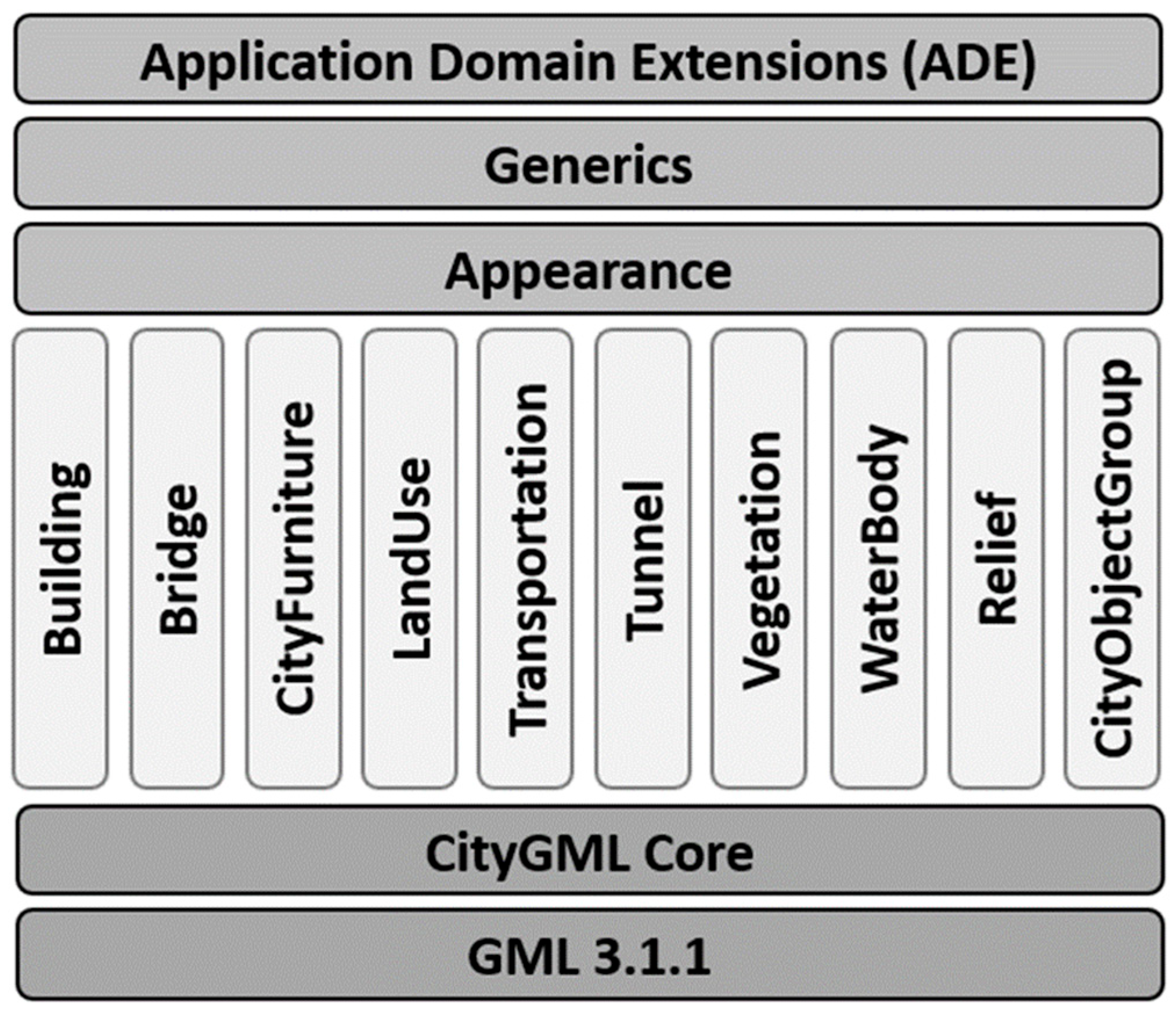
CityGML 2.0 consists of a core module, modules for extending the information model, a module for appearance and ten thematic modules for different types of objects (Figure 2). The data in CityGML can be stored in different levels of detail (LOD). For some thematic modules, the LODs are well defined, such as for Building [53] and Transportation [54], while for other modules, including LandUse, there is no consensus on the LOD definition.
There have been several studies on how to handle the thematic modules within CityGML, e.g., Building [53,55], Transportation [56,57,58] and Vegetation [59,60]. The focus in this study is on LC and elevation data, which are described in detail below.
Figure 2. Overview of the CityGML 2.0 modules. The vertical boxes show the thematic modules (following [12], modified from [61]).
Ijgi 14 00328 g002

2.3.2. Land Cover Data in CityGML

CityGML has a module LandUse that can be used for storing both LC and LU data. In addition, LC data is stored in other modules, e.g., Vegetation and Transportation, which means there will be redundancy if the LandUse module is used to create an LC partition of a city. One alternative, explored in this study, is to store LC data in several modules and combine data from those modules to create an LC partition. With this approach, surfaces that do not naturally fit in any other module, e.g., paved surfaces in schoolyards that are neither Vegetation nor Transportation surfaces, are stored in the LandUse module. This alternative requires that the code lists in all the modules are tailored to support the LC classification used and that surfaces in the LandUse module are separated into LC and LU surfaces.

2.3.3. Elevation Data in CityGML and Other Urban Digital Twin Models

Within CityGML, elevation data can be stored in the Relief module represented as GRID, Triangulated Irregular Network (TIN), break lines and point clouds [12,13]. However, this module is rarely used even though there are some examples (e.g., [62]). One reason is that elevation data in the Relief module is stored as Geography Markup Language (GML) geometries, which is space-intensive; there are significantly more efficient storage models such as LAS files for point clouds and GeoTIFF for GRID. Furthermore, the TIN representation in the Relief module has some limitations [14]. More efficient TIN structures, among other things, were proposed by Kumar et al. [63], which could technically be implemented as a CityGML ADE.
Elevation can also be stored in other CityGML modules using 2.5D and 3D surfaces by adding elevation to, e.g., road surfaces (in the Transportation module), vegetated areas (in the Vegetation module), and water bodies (in the WaterBody module). Furthermore, elevation is stored as 3D objects in the Building, Bridge and CityFurniture modules. The challenges here lie in achieving a consistent and topologically correct description of ground elevation and 3D objects where it does not exist: (a) holes or overlaps between (2.5D) surfaces, (b) 2.5D surfaces that do not meet vertically, and (c) 3D objects that do not connect to 2.5D surfaces, e.g., buildings that do not connect to the ground.
To solve challenges (a) and (b), it is possible to share geometric objects in CityGML via xLink, but this is a complex structure that is difficult to implement in practice [64]. To practically solve challenge (c), terrain intersection curves (TICs) are sometimes used. TICs are used in, e.g., the Building module to store the 3D line geometry that is the intersection between a building’s footprint and the ground surface (represented by, e.g., a TIN). That is, the TIC is a 3D break line/geometry, and there are methods to generate these topologically correctly [11]. TICs are important to ensure correct topological relationships between 3D objects and the 2.5D terrain in the city model, and are thus important for several purposes, e.g., for flood analysis [65] and visualizations [66]. However, it should be pointed out that few 3D city models store TICs; a survey found that only three 3D city models (Espoo, Hamburg, Sofia) out of twenty models examined used TICs [66].
Lehner et al. [15] created a 3D city model of Vienna where they stored elevation data in, e.g., the LandUse, Transportation and WaterBody modules (but not Relief) as multisurfaces (MultiSurfaces) and 3D objects (e.g., buildings). To create a hole-free LC partition when all 2.5D objects are added together without 3D city objects, a virtual surface (added in an ADE and named LandUseClosureSurface) is used for land areas covered by, e.g., buildings; the outer edges of these virtual surfaces then coincide with a TIC [15].
CityGML can handle elevation data in several LODs, regardless of whether the elevation data is stored in the Relief module or other modules. There are no definitions of these LOD levels in the CityGML conceptual model [13], but there are proposals of such definitions, e.g., given by Kumar et al. [67]:
LOD0—A 2.5D terrain elevation model (which cannot handle vertical surfaces).
LOD1—A surface elevation model that can handle vertical surfaces.
LOD2—A 2.5D ground elevation model where footprints of semantic objects have been integrated.
LOD3—A surface elevation model that can handle vertical surfaces where semantic objects from other CityGML modules have been integrated.
However, it can be argued that this definition is not optimal because it mixes terrain elevation models with surface elevation models; another possibility would be to handle terrain and surface model separately, since there is a need for both types of models in different levels of detail (using a similar argument as used for separating outdoor and indoor information in the LOD definition in the Building module in CityGML 3.0 [13]).
In this study, as well as in many other 3D city model studies, the TIN model is mainly generated by creating a triangulation of thinned point clouds (collected by airborne laser scanning or photogrammetry). The disadvantage with this approach is that the triangles can vary in size and form (and in the worst case, they are not watertight), which makes them unsuitable for some urban digital twin applications. One example is wind simulations using techniques such as computational fluid dynamics (CFD). For this type of application method, generating well-formed triangles (meshes) optimized for the simulations is required (see, e.g., [68,69]).

2.3.4. Swedish Profile of CityGML—3CIM

The Swedish 3D city model profile 3CIM is based on a CityGML 2.0 ADE and semantically thin, mainly extending CityGML with attributes to harmonize with national standards; information should be stored and maintained at the source, such as operational systems (e.g., building permit systems) and external registers (e.g., the National Road Database) and linked to 3CIM. For details about ver. 1.0 of 3CIM, see Uggla et al. [16]. In this study, we use 3CIM ver. 2.0, which is defined in a UML model, following best practices for creating a CityGML ADE [70,71] and available on GitHub (https://github.com/3CIM/3CIM2.0, accessed on 20 August 2025). The only major update that is relevant for this study is that the LandUse module was updated to better handle LC data (see Section 3.4).

3. Methods

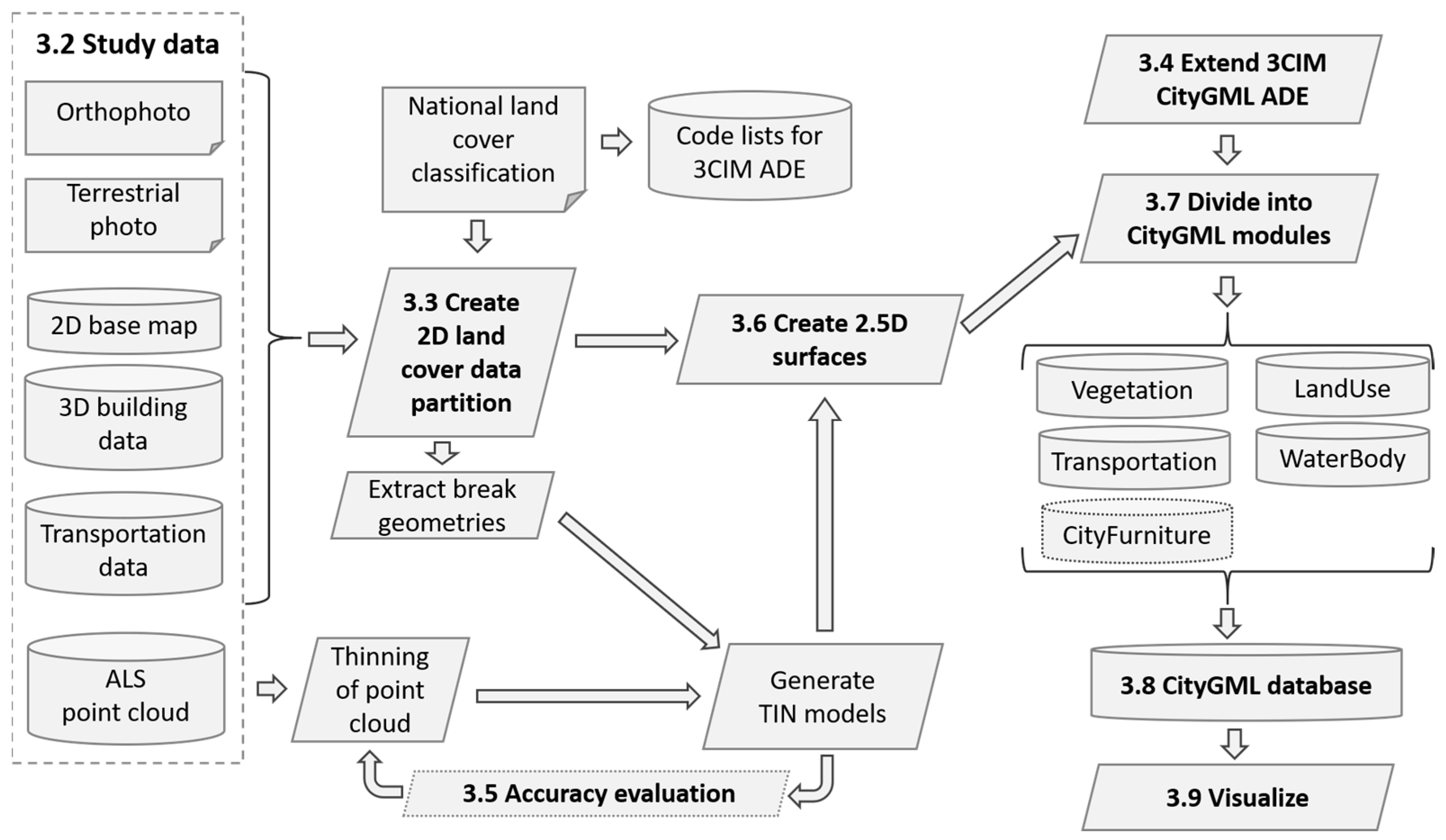
This study includes all steps from creating the LC data for the study area, converting it to CityGML/3CIM data and storing it in the 3DCityDB database, to create a final visualization (Figure 3). The data used in the study is described in Section 3.2. The creation of the LC partition is described in Section 3.3 and the extension of the 3CIM ADE in Section 3.4. The LC and elevation data are integrated by draping the LC partition on a TIN, modeled from a thinned point cloud, to create 2.5D LC surfaces. Before the final TIN was created, we performed an accuracy evaluation of TIN models created from point clouds with different levels of thinning. The creation of TIN models and evaluation are described in Section 3.5 and the creation of 2.5D LC data in Section 3.6. The LC data was then divided into CityGML modules (Section 3.7), stored in a CityGML database (Section 3.8) and visualized in LOD2 (Section 3.9).

3.1. Study Area

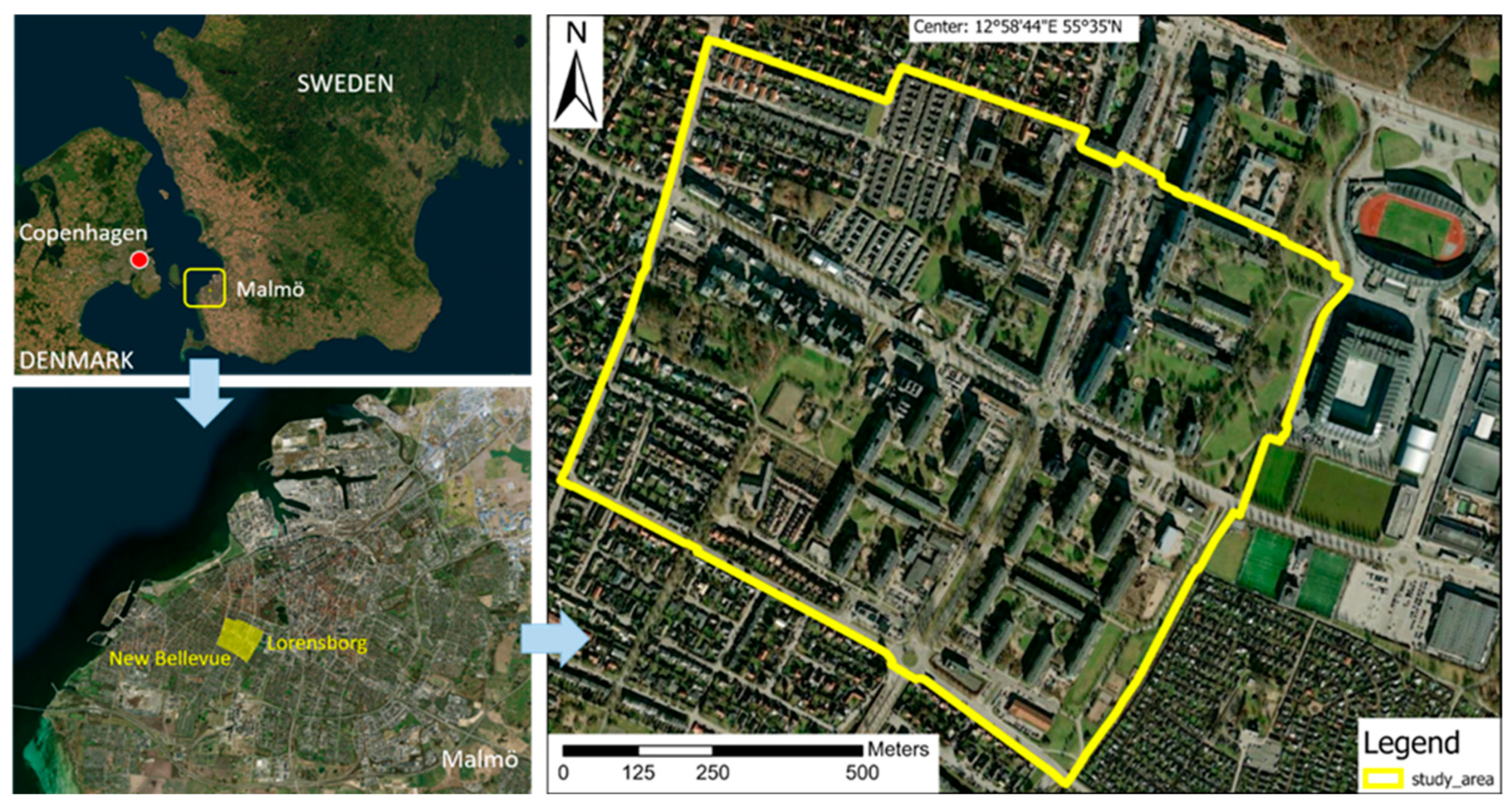
The study area encompasses the new Bellevue and Lorensborg neighborhoods of the Malmö municipality in southern Sweden and covers an area of approximately 945,000 m2 (Figure 4). The area is dominated by residential buildings (villas as well as 3–6-story buildings) with some commercial and educational buildings. Moreover, the study area is characterized by varying land cover types comprising both vegetated and built-up areas and has a relatively flat topography.

3.2. Study Data

The geospatial data used in this study are described in Table 1. All data, except the terrestrial photographs which were taken by the authors, are owned by the city of Malmö. For the east part of the study area, buildings and transportation data were reused from 3CIM ver. 1.0 test data [16].

3.3. Create 2D Land Cover Map Partition

The 2D LC dataset used in this study was generated by manually digitizing Malmö municipality’s base map in ArcGIS Pro (www.esri.com) to form polygons from various line objects (such as roads, biking paths, walking paths, pavements, parks, etc.) or polygons (building footprints) and assigning an LC class to each digitized polygon [26]. For a portion of the study area, major road polygons were derived from Malmö municipality’s 3CIM test area [16]. Road data for the remaining areas were digitized by overlaying the corresponding line objects from the municipality’s base map on orthophotos. To represent the ground surface material more accurately, the digitized LC layer was enhanced by incorporating data from terrestrial photos, as well as imagery from Google Earth and Google Street View. The creation of detailed LC layers is not easy. Besides the time required for manual digitization, the fact that the ancillary datasets have different updating frequencies, i.e., biannually updated orthophotos and continuously updated base maps, complicates the process even further. In this instance, the datasets containing the most recent information, i.e., terrestrial photos and base maps, were prioritized.

3.4. Extending the LandUse Model in 3CIM

The limitation with the LandUse module for the method presented in this study is that LC and LU surfaces are not separated. Hence, the 3CIM ADE was extended by creating the subclass LandCover to the LandUse module (Figure 5) to facilitate storage of LC data and LU data in separate classes. Furthermore, the LandUse module was extended with a LandCoverClosureSurface, a virtual 2.5D surface to fill holes from 3D objects in the LC data, e.g., for building footprints (cf. [15]). To link a LandCoverClosureSurface feature to its corresponding 3D object, an attribute originalObjectUUID (ursprungsObjektUUID in Swedish; Figure 5) was added. The originalObjectUUID will act as a foreign key to the UUID of the 3D object it represents.
The new UML model was created in Enterprise Architect (https://www.sparxsystems.eu/, accessed on 20 August 2025) and transformed to an XML schema (xsd-file) using the ShapeChange tool (https://shapechange.net/, accessed on 20 August 2025). The xsd-file is available here: https://github.com/3CIM/3CIM2.0/tree/main (accessed on 20 August 2025).

3.5. Thinning of Point Cloud and Accuracy Evaluation of TIN Models

A TIN model is formed by a triangulation of 3D points, e.g., in a point cloud from airborne laser scanning (ALS). The ALS point clouds are generally so dense that only a subset of the points is included. It is important that the points included in the TIN model preserve important structures in the terrain, for example ridges and human-made structures such as the topography of roads [72,73]. Break geometries, which force some points and edges to be included in the TIN, are often used in the production of TIN to maintain the structures [73,74]. Break geometries also reduce the need for points in the model by providing clear, well-measured geometries to support the TIN model [72,75].
The TIN model used to create 2.5D LC data in this study was created from an ALS point cloud and break geometries from the 2D LC data in two steps, where the point cloud was thinned in both steps. In step 1, 3D break geometries were created by first creating a temporary TIN model from the original ALS point cloud, then the boundaries of the 2D polygons in the LC data were draped on the TIN to obtain the 3D break geometries. In step 2, the final TIN model was created from the ALS data with the 3D break geometries from step 1 as constraints, and the 2.5D LC data was created by draping the 2D LC data on this TIN. The processing was performed with the extract, transform, and load (ETL) tool Feature Manipulation Engine (FME; www.safe.com/).
The point cloud in the study area is dense (35–40 points/m2), which entails that not all points can be used in the TIN models for performance reasons. To decide how many points should be used in the triangulation (step 2), we studied how the vertical accuracy was influenced by the number of points used to create the TIN model; various thinning strategies, both with and without break geometries, were tested. With fewer points included in the TIN, the vertical distance between the points (not included in the triangulation) and the triangulated surface increases. The total vertical uncertainty depends on both the positional uncertainty in the point cloud and the uncertainty created by using a subset of the points [76,77]. The total uncertainty was calculated with the error propagation formula:
σ y = σ x t h i n n i n g 2 + σ x p o s i t i o n a l   a c c u r a c y 2
where σy is the total uncertainty, σx,thinning is the uncertainty due to point selection and σx,positional accurace is the vertical accuracy in the point cloud.
In this study, we accepted a total vertical uncertainty up to 0.1 m, which implies that the uncertainty generated by the point selection must be within a few cm. For further details, see Andersson [78].

3.6. Creation of 2.5D Land Cover Surfaces

The LC and elevation data were integrated by draping the 2D LC data on the TIN to create 2.5D LC surfaces, where the TIN was created from the thinned point cloud, with the LC polygons as break geometries (see Section 3.5). This procedure was performed in FME; see Appendix A for details.
In this step, the buildings were included in the LC data as building footprints in 2.5D (3CIM ADE class LandCoverClosureSurface). The LandCoverClosureSurface objects were linked to correct 3D building objects in the next step, when the LC data was split into CityGML modules (Section 3.7).
Vertical features, such as retaining walls, that could not be modeled by draping polygons on the TIN were manually digitized in ArcGIS Pro version 3.2 from ESRI (www.esri.com) and assigned to the CityFurniture module in CityGML.

3.7. Divide the LC Data into CityGML Modules

The 2.5D LC surfaces were divided into the CityGML modules Transportation, Vegetation, WaterBody and LandUse (in the subclass LandCover in the 3CIM ADE) based on the NS LC class and the mappings in Table 2 (see below for details). The retaining walls (CityFurniture) were already assigned to the correct CityGML module.
FME (TestFilter transformer) was used to divide the LC data into CityGML modules. The xml schema (xsd) file for the 3CIM ADE (see Section 3.4) was used to extend the FME CityGML writer and the data was saved as a CityGML file. In Table 2 and the text below, we have translated the attribute values in NS LC to English.

3.7.1. Transportation

The NS LC classes asphalt, sett (paving) and cobblestone were mapped to the Transportation module (TrafficArea only) and the LC class was added as surface material (attribute SurfaceMaterial). To enable storage and import/export to/from 3DCityDB, the TrafficArea and AuxilliaryTrafficArea (from 3CIM ver. 1.0 test data [16]) objects were assigned to Road (subclass of TransportationComplex) objects with one Road object for each TrafficArea and AuxilliaryTrafficArea.

3.7.2. Vegetation

The NS LC classes grass and bushes were mapped to the Vegetation module in CityGML as PlantCover.

3.7.3. WaterBody

The NS LC classes pool and pond were mapped to the WaterBody module in CityGML.

3.7.4. LandUse

The remaining LC classes were mapped to the LandCover class (the 3CIM subclass of LandUse; see Figure 5), namely concrete, natural stone, gravel bed, excavated land, artificial turf, rubber surface and paving stone. In addition, several of the surfaces that were mapped to the Transportation module based on surface material had to be manually assigned to the LandCover module instead; these were mainly asphalt surfaces, e.g., in schoolyards or courtyards that do not belong to the Transportation module. Furthermore, the building footprints in 2.5D (3CIM ADE class LandCoverClosureSurface) were linked to the original 3D buildings via a spatial join to set the value of the original object UUID attribute (denoted ursprungsObjektUUID in Figure 5).

3.8. Storing the Data in a Database

In this study, we stored the data in 3DCityDB where the 3CIM ADE was implemented by the company Virtual City Systems based on the XML schema (xsd-file) described in Section 3.4. The database was installed on top of a PostgreSQL/PostGIS installation, and the 3DCityDB ADE Manager was used to import the 3CIM ADE into 3DCityDB.
The Importer/Exporter tool for 3DCityDB was used to import and export data to/from the database and an FME script was developed to automate the workflow. The FME script runs the Importer/Exporter via Command Line Interface (CLI) and communicates directly with the database via SQL, e.g., to extract metadata (ADE version) that is saved together with the exported CityGML data.
To enable realistic visualization, additional objects were added to the LC data: 3D buildings (Building module), solitary trees (Vegetation module) and walls (CityFurniture module). Solitary trees and walls were obtained from 3CIM ver. 1.0 test data [16] and LOD2.1 3D buildings from 3CIM ver. 1.0 test data and the City of Malmö. The objects were added to the CityGML file with the LC data in FME and all data was imported to 3DCityDB at the same time with the Importer/Exporter tool.

3.9. Visualize the Data in 3D

The data was exported from 3DCityDB and a 3D visualization in LOD2 was performed with Unreal Engine (UE) version 5.2.2 (https://www.unrealengine.com/en-US, accessed on 20 August 2025) following the workflow described below.

3.9.1. Data Pre-Processing

The data was first exported from 3DCityDB as CityGML (gml-file) and read into FME to convert it to the UE-compatible obj-format. The following steps were performed:
  • Attributes were saved as csv-files.
  • Positions of point objects (trees) were exported from the gml-file as csv.
  • The data was transformed to a local coordinate system.
The files were grouped into separate folders based on the CityGML/3CIM object type (TrafficArea, AuxilliaryTrafficArea, LandCover, etc.) and saved as top-level folders. For each object type, one sub-folder for each surface material (i.e., LC class in this study) was added. For the purpose of this study, we generalized the output to a total of 10 LC classes. The geometry of each object (except for point objects) was then exported with gml:id as the unique identifier.
For objects that are represented as points (here only trees as SolitaryVegetationObject), the offset from the coordinate reference system to the local coordinate system was made and the coordinates were extracted before being exported.

3.9.2. Visualization in Unreal Engine

A project was created in UE and the following items/settings were prepared before any data was imported:
  • Basic lighting and associated settings;
  • Material library containing roughly 10 materials;
  • User Interface (UI) and camera with associated controls;
  • Function for replacing point data with meshes;
  • Function and UI for displaying attributes.
The geometries (3D models) were imported to UE following the same structure as we used to write the files above. Since the extent of the study is small, all data could be imported at once; for larger areas, a recommendation would be to batch process.
All objects were placed at the same position (X, Y, Z) in the UE scene to maintain their relative positions. This was performed folder by folder, and groups were created in UE Outliner for easier access later. With this structure, all 3D models within a folder could be selected and have the material assigned at the same time. This process could also be automated using the attribute information directly within UE, which would be advantageous when working with larger datasets and a larger number of materials but has not been tested as part of this study.
For the csv-files, “Data Structures” were created within UE so they could be read correctly. The structures were created by defining the correct data type (float, string, etc.) for each attribute. These were then used in the already existing functionality to place models and create references for the attributes to the UI.

4. Results

The 3D LC data created in this study resulted in a file size of 17 MB in gml-format, including around 1500 LandCover objects, 500 LandCoverClosureSurface objects (buildings), 2300 Vegetation (PlantCover) objects, 800 Transportation (TrafficArea, AuxilliaryTrafficArea) objects and 20 objects each in the WaterBody and CityFurniture modules. When the 3D buildings (500 objects; solid and surface representation), trees (2000 objects) and walls (50 objects) were added to the CityGML file, the size increased to 49 MB.

4.1. Accuracy Evaluation of TIN Models

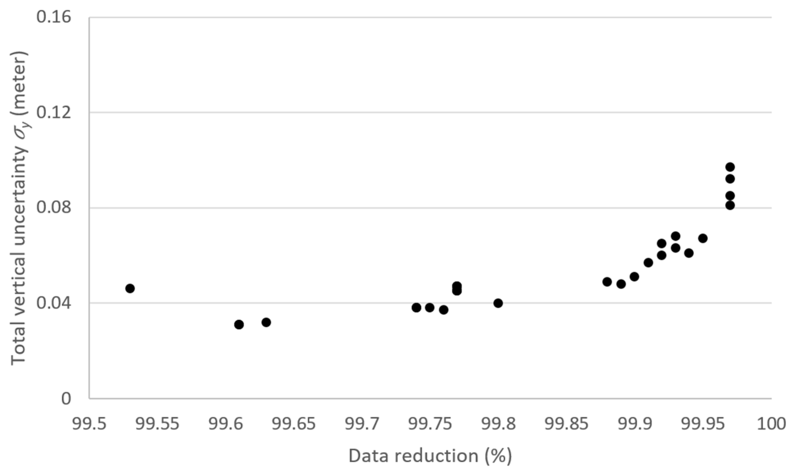
In this part, several methods to generate 2.5D surfaces from the dense ALS point cloud were tested. The tests revealed that the point cloud could be substantially reduced when creating a TIN if a total vertical accuracy (Equation (1)) of 0.1 m was accepted. From Figure 6, we can observe that more than 99.9% of the points can be removed if break geometries are used. The main result from these tests was experience with methodologies, including parameter settings and usage of break geometries, for generating TIN models.

4.2. CityGML Modules and Land Cover Partition

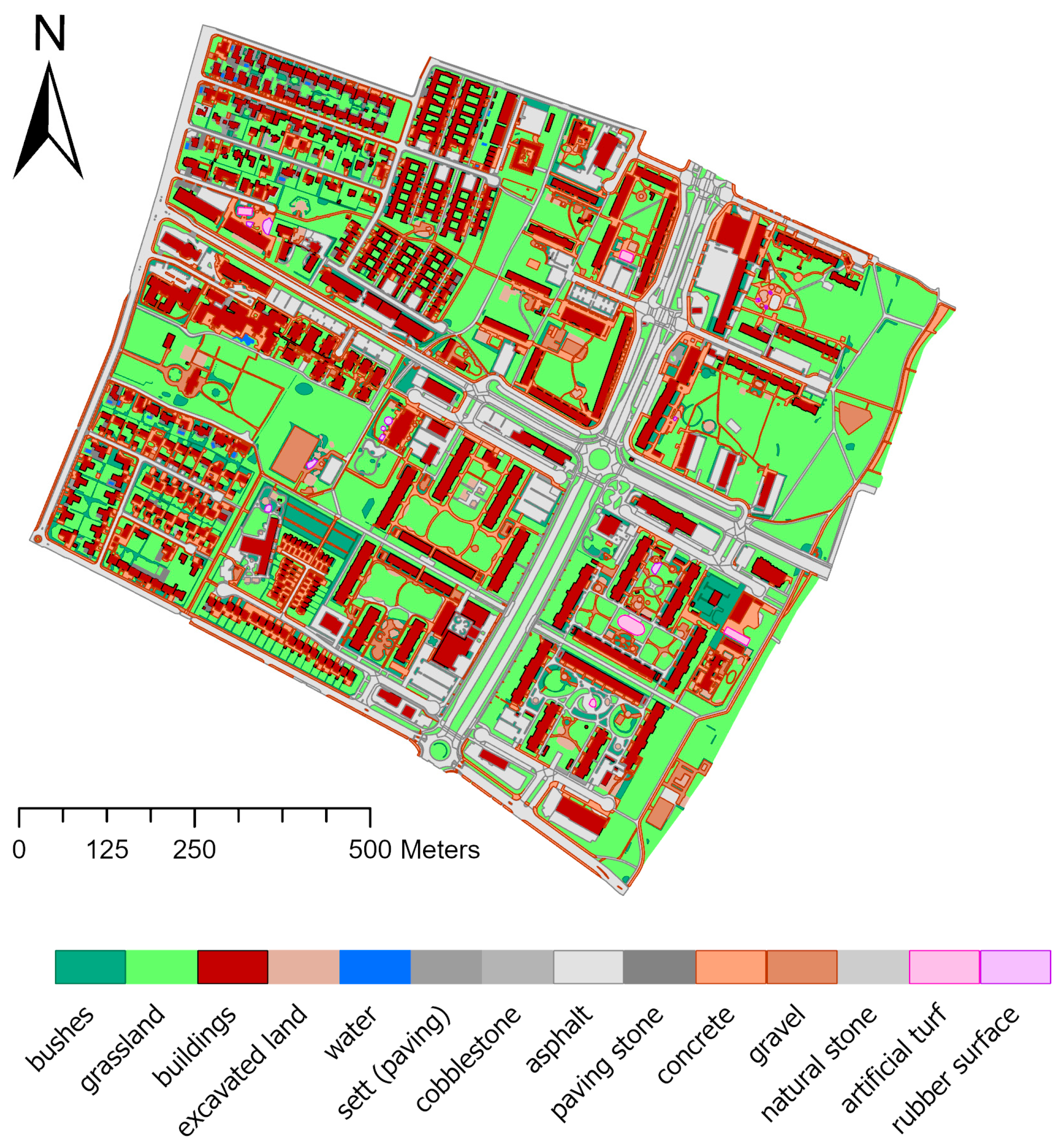
In the left part of Figure 7, the LC data in the CityGML modules LandUse, Transportation, Vegetation, WaterBody and CityFurniture (not visible in 2D) are shown. These modules, with the footprint of 3D buildings included as LandCoverClosureSurface objects in the LandUse module, could successfully be merged to a complete 3D LC partition including five NS LC classes on level 3, namely bushes, grassland, buildings, hard/impervious surfaces and water (Figure 7, right side). Figure 8 illustrates the land cover data on the most detailed level used in this study.

4.3. Three-Dimensional Visualization

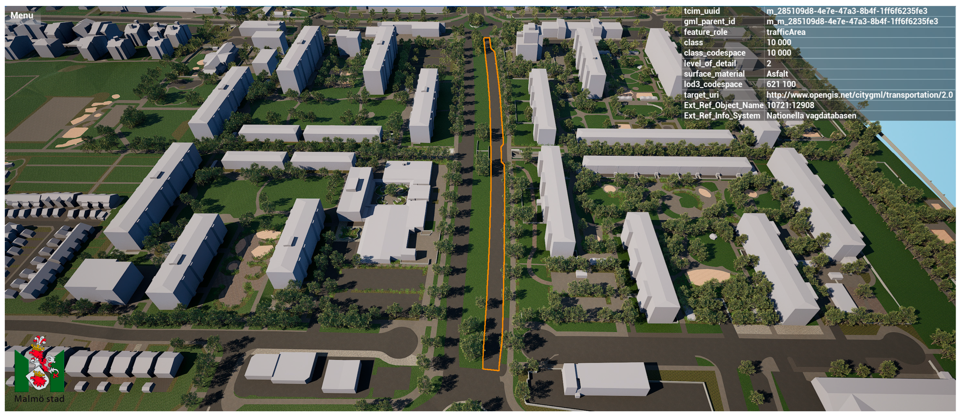
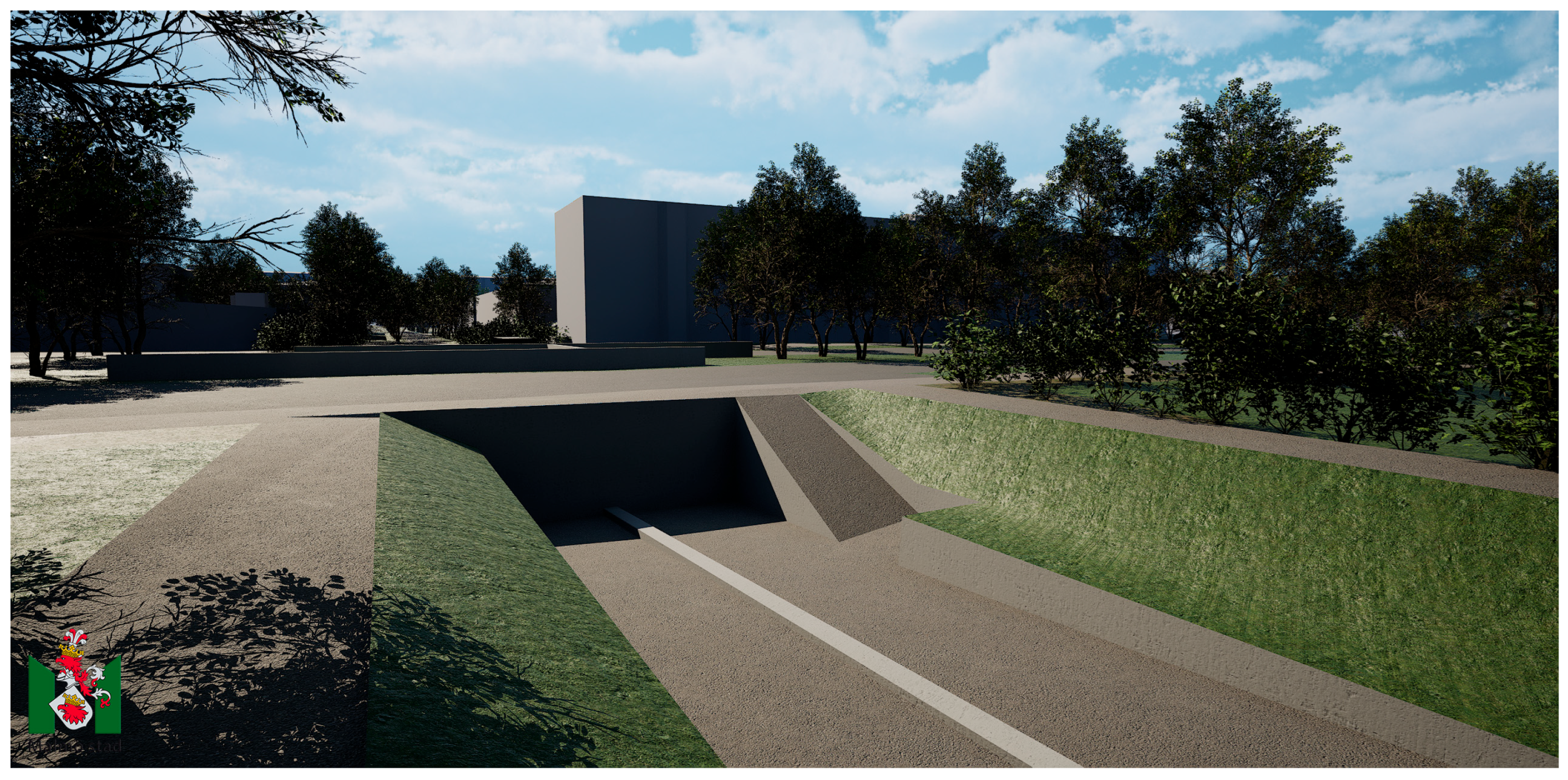
The CityGML/3CIM data, exported as a gml-file from 3DCityDB, was visualized in Unreal Engine in LOD2. Figure 9 shows an overview of one part of the study area with one road selected (highlighted with an orange boundary) to illustrate how the attribute values of selected objects are displayed. Figure 10 is a zoomed-in view over a small area.

5. Discussion

In this study, we demonstrate how a 3D LC partition can be created by storing LC data in the CityGML modules Transportation, Vegetation, WaterBody, LandUse and CityFurniture as 2.5D/3D multisurfaces. The main advantage of this approach, rather than utilizing the Relief module in CityGML, is the integration of the elevation data in the LC data. This is not only of interest to create nice visualization, but also a prerequisite for some simulations (e.g., some hydrological models used for flood estimations).
Combining the CityGML modules to create a 3D LC partition worked well, but there were some issues when mapping the LC partition to CityGML modules. For most LC classes, the mapping worked well. The LC class that resulted in most errors was asphalt, which was mapped to the Transportation module; however, several surfaces with asphalt, e.g., in schoolyards or courtyards that do not belong to the Transportation module, had to be manually changed to the LandUse module. Other LC classes that were mapped to the incorrect CityGML module were also related to the Transportation module; stone surfaces such as cobblestone and sett, which can belong to both Transportation and LandUse; and grass or bushes in roundabouts and median dividing, that should be mapped as Transportation (AuxilliaryTrafficArea) instead of Vegetation.
For the WaterBody, Vegetation and LandCover modules, the process to divide LC data into CityGML modules was fairly simple since the objects were handled individually. For the Transportation module, it is a complex process since individual TrafficArea and AuxilliaryTrafficArea objects need to be grouped into TransportationComplex. As an example, a Road (subclass of TransportationComplex) might consist of several TrafficArea objects (e.g., lanes for cars and walkways) and AuxilliaryTrafficArea objects (e.g., grass median dividing) [12]. In this study, we did not group the individual TrafficArea and AuxilliaryTrafficArea objects into TransportationComplex; instead, we created one Road object for each TrafficArea and AuxilliaryTrafficArea to enable storage and Import/Export to/from 3DCityDB. However, the recommendation in 3CIM is that TrafficArea and AuxilliaryTrafficArea are grouped into sections following CityGML 3.0 [13,54].
To avoid confusion between land cover and land use, we added a subclass LandCover to the CityGML module LandUse. The main motivation for this is that storing LC data in a separate class facilitates the creation of the LC partition. In addition, separating LC from LU means there will not be overlapping surfaces in the same class, for example paved areas (LC) inside a park (LU). If adapting the 3CIM ADE to CityGML 3.0, which introduced physical and logical spaces [13], the class LandCover could be modeled as physical spaces (what exists on the ground) and LandUse as logical spaces (how the areas are used).
In this study, we extended the 3CIM ADE with a LandCoverClosureSurface in a similar fashion to Lehner et al. [15] to fill the holes in the LC data below 3D objects such as buildings. LandCoverClosureSurface has an attribute (UrsprungsObjektUUID in Figure 5) to link the 2.5D surface with the original 3D object. In simulations where the materials of facades (e.g., noise simulations [26]) or roofs (e.g., flooding [35]) must be known, the actual material can be derived from the original 3D building object if the ADE is extended with attributes for surface materials in the Building module.
Vertical surfaces (e.g., retaining walls) that are not actual land cover could also have been modeled as LandCoverClosureSurface. In this study, we decided to include the retaining walls (part of the CityFurniture module) in the 2.5D LC partition instead. The advantage of this is that we avoid redundancy, i.e., there is no need to store the geometry of the retaining walls both as CityFurniture and LandCoverClosureSurface, and all attributes from the original CityFurniture object are available with the LC data, which is an advantage for, e.g., noise and flood simulations. However, it needs to be decided which objects from the CityFurniture module should be included in the LC partition; in our study area (Figure 4), the only vertical structures were retaining walls.
Since this study focuses on land cover, the most relevant class in the Vegetation module is PlantCover. Some analyses, e.g., daylight simulations [59] and urban climate [39], also require 3D data on trees. In CityGML, trees can be stored in the Vegetation module as SolitaryVegetationObjects, which is also the approach taken within 3CIM and tested in this study when importing trees for the 3D visualization.
No attempt to define LODs for the LandUse module in a similar fashion to Building [53] and Transportation [54] was made. However, for the Transportation module, LOD2 is required since the land cover information is stored as SurfaceMaterial, and that attribute is only available in LOD2 or higher (in the TrafficArea and AuxilliaryTrafficArea classes); in lower LODs, the TrafficArea and AuxilliaryTrafficArea objects are aggregated into TransportationComplex, which only gives information about land use [12,13]. Hence, the recommendation in 3CIM is to use LOD2 for the land cover data.
A major issue in this study was creating the 2.5D/3D surfaces from the 2D LC data with the ALS point cloud as the only source for elevation. This was performed by creating a TIN from the ALS data and draping the 2D LC data on the TIN. However, the method has limitations in steeper areas and is insufficient for vertical surfaces, such as retaining walls, which cannot be modeled by draping on a TIN. In this study, we conducted some manual digitizing, which is time-consuming. To facilitate better 3D modeling, improvements should be made to the measuring guidelines for the 3D city model (see examples of such guidelines in [79,80]). In these guidelines, it should be stated that the upper part of retaining walls or edges of roads and biking paths, etc., should be measured and include elevation; then, it would be possible to automatically generate the 3D surfaces. It could also be interesting to use methods to generate TIN models developed for wind simulations in urban digital twins, which could create better-formed triangles to enhance both simulations and visualizations [68,69]. If this approach is taken, it would be a requirement that land cover boundaries, as well as steep edges, would act as break geometries in the TIN generation.
In this study, we classified the land cover according to a preliminary Swedish national specification. The main motivations for using the Swedish classification are that it facilitates data sharing via the national geoportal and it includes only LC classes. Furthermore, the classification scheme needs to be more detailed than, e.g., CORINE, and the code lists for classification at level 4 created within 3CIM can be used if a fourth level is developed for the Swedish classification system. Since CORINE includes LU classes, it would not be straightforward to add a level 4; for example, asphalt would belong to several of the level 3 classes in CORINE (e.g., Continuous urban fabric, Industrial or commercial units, and Airports).
The classification scheme that is used does not influence the overall methodology of this study. However, using a standard classification scheme is a major advantage for many analyses and simulations since the LC classes (materials) can be linked to code lists to map materials to physical property values. This would be one more step towards fully automating the execution of simulation processes using semantic 3D city models as input. For example, to conduct noise simulations, it is important that accurate flow resistivity values (simplified: if it is a soft or hard surface in terms of noise modeling) are measured for the land cover classes [26,81]. To make this work in practice, there needs to be cooperation between noise experts (as well as other domain experts) and the geospatial community when defining the land cover specifications.

6. Conclusions

In this study, we have established methods to integrate land cover (LC) data, elevation data and 3D objects to create a 3D LC representation in a semantic 3D city model. As part of the work, we have developed a framework for dividing LC data between the CityGML modules Transportation, Vegetation, WaterBody and LandUse. The LC data is draped on a TIN generated from an airborne laser scanning point cloud to generate 2.5D LC surfaces. To generate a complete 3D partition, we added vertical structures, which in our study area were retaining wall objects (stored in the CityFurniture module). That is, the elevation data is integrated (as multisurfaces) in the LC data, rather than being stored separately in the Relief module. We demonstrate that this approach enables nice visualizations; another main advantage of this approach is that the semantic 3D city model could be used as input to simulations (flood, noise, etc.) where integrated elevation and land cover data improves the simulation results or is even required. Finally, we stress the importance of using good classification schemes for LC data. In our study, we have used a preliminary national specification for land cover, an approach that will likely enable the city model data to work as input to simulations since there will be recommendations for parameter settings for infiltration capacities, acoustic properties, etc., based on the LC classes in this scheme.

Author Contributions

Conceptualization, Lars Harrie and Per-Ola Olsson; methodology, all authors; investigation, Per-Ola Olsson, Axel Andersson, Erik Lökholm and Axel Loreman; data curation, Per-Ola Olsson and Karolina Pantazatou; writing—original draft preparation, Per-Ola Olsson and Lars Harrie; writing—review and editing, all authors; visualization, Axel Loreman, Karolina Pantazatou and Per-Ola Olsson; supervision, Lars Harrie and Per-Ola Olsson; project administration, Lars Harrie and Maria Uggla; funding acquisition, Maria Uggla. All authors have read and agreed to the published version of the manuscript.

Funding

The 3CIM project is part of the Smart Built Environment program funded by Formas, Sweden’s Innovation Agency Vinnova, and the Swedish Energy Agency, grant number Formas-2023-00094. Creation of LC data was a cooperation with the project “Increase the potential for energy and noise simulations when planning urban densification”, funded by Formas 2020-01460. Financial support has also been provided by the cities of Stockholm, Gothenburg, and Malmö, as well as by Lund University (Sweden).

Data Availability Statement

Data are available here: https://github.com/3CIM/3CIM2.0/tree/main/testdata (accessed on 20 August 2025).

Acknowledgments

Thanks to the city of Malmö for providing all the data and colleagues in the 3CIM project for their work and fruitful discussions. Thanks to Claus Nagel and his colleagues at Virtual City Systems for their support with developing the 3CIM ADE and implementing it in 3DCityDB.

Conflicts of Interest

The authors declare no conflicts of interest. The funders had no role in the design of the study; in the collection, analyses, or interpretation of data; in the writing of the manuscript; or in the decision to publish the results.

Abbreviations

The following abbreviations are used in this manuscript:
3CIMNational profile of CityGML (Sweden)
ADEApplication domain extension
LCLand cover
LODLevel of detail
LULand use
NSNational specifications for geodata (Sweden)
NS LCNational classification scheme for LC data (Sweden)
TICTerrain intersection curve
TINTriangulated irregular network
UEUnreal Engine (here version 5.2.2)

Appendix A. Thinning Procedure and Creation of 2.5D Land Cover Surfaces

The thinning procedure was performed in FME in two steps, where part of the thinning was conducted in both steps:
  • Step 1—creating 3D break lines:
A PointCloudThinner was applied to remove every 2nd point. Then the point cloud was further thinned with a PointCloudSimplifier (Filter Ratio = 0.3), and a TINGenerator (Surface Tolerance = 0.5) was used to create the TIN. Finally, the boundaries of the LC polygons were draped on the TIN with a SurfaceDraper (Surface Tolerance = 0; Drape Method = Vertex) to create the 3D break geometries.
  • Step 2—creating 2.5D LC data:
A PointCloudThinner was applied to remove every 2nd point (applied to the original point cloud). Then a digital terrain model (DTM) with a spatial resolution of 1 m was created with a RasterDEMGenerator (Surface Tolerance = 0.5), and a TIN was created with a TINGenerator (Surface Tolerance = 0.3 and break lines from step 1). The TIN was created from a DTM to obtain a more even spatial distribution of vertices. Finally, the 2.5D LC data was created by draping the 2D LC data on the TIN with a SurfaceDraper (Surface Tolerance = 0; Drape Method = Vertex).

References

  1. Seto, T.; Furuhashi, T.; Uchiyama, Y. Role of 3D City Model Data as Open Digital Commons: A Case Study of Openness in Japan’s Digital Twin “Project Plateau”. Int. Arch. Photogramm. Remote Sens. Spat. Inf. Sci. 2023, XLVIII-4/W7-2023, 201–208. [Google Scholar] [CrossRef]
  2. Helsinki. The Kalasatama Digital Twins Project, the Final Report of the KIRA-Digi Pilot Project. 2019. Available online: https://www.hel.fi/static/liitteet-2019/Kaupunginkanslia/Helsinki3D_Kalasatama_Digital_Twins.pdf (accessed on 22 October 2024).
  3. Schrotter, G.; Hürzeler, C. The digital twin of the City of Zurich for urban planning. PFG 2020, 88, 99–112. [Google Scholar] [CrossRef]
  4. Dembski, F.; Wössner, U.; Letzgus, M.; Ruddat, M.; Yamu, C. Urban Digital Twins for Smart Cities and Citizens: The Case Study of Herrenberg, Germany. Sustainability 2020, 12, 2307. [Google Scholar] [CrossRef]
  5. Ketzler, B.; Naserentin, V.; Latino, F.; Zangelidis, C.; Thuvander, L.; Logg, A. Digital Twins for Cities: A State of the Art Review. Built Environ. 2020, 46, 547–573. [Google Scholar] [CrossRef]
  6. Kephalopoulos, S.; Paviotti, M.; Anfosso-Lédée, F. Common Noise Assessment Methods in Europe (CNOSSOS-EU); Publications Office of the European Union: Brussels, Belgium, 2012. [Google Scholar]
  7. Vieux, B.E.; Vieux, B.E. Distributed Hydrologic Modeling Using GIS; Springer: Dordrecht, The Netherlands, 2001; pp. 1–17. [Google Scholar]
  8. Rahman, M.A.; Franceschi, E.; Pattnaik, N.; Moser-Reischl, A.; Hartmann, C.; Paeth, H.; Pretzsch, H.; Rötzer, T.; Pauleit, S. Spatial and temporal changes of outdoor thermal stress: Influence of urban land cover types. Sci. Rep. 2022, 12, 671. [Google Scholar] [CrossRef]
  9. Harrie, L.; Kanters, J.; Mattisson, K.; Nezval, P.; Olsson, P.-O.; Pantazatou, K.; Kong, G.; Fan, H. 3D City models for supporting simulations in city densifications. Int. Arch. Photogramm. Remote Sens. Spat. Inf. Sci. 2021, XLVI-4/W4-2021, 73–77. [Google Scholar] [CrossRef]
  10. Gonzalez-Caceres, A.; Hunger, F.; Forssén, J.; Somanath, S.; Mark, A.; Naserentin, V.; Bohlin, J.; Logg, A.; Wästberg, B.; Komisarczyk, D.; et al. Towards digital twinning for multi-domain simulation workflows in urban design: A case study in Gothenburg. J. Build. Perform. 2024, 18, 311–332. [Google Scholar] [CrossRef]
  11. Yan, J.; Zlatanova, S.; Aleksandrov, M.; Diakite, A.A.; Pettit, C. Integration of 3D objects and terrain for 3D modelling supporting the digital twin. ISPRS Ann. Photogramm. Remote Sens. Spat. Inf. Sci. 2019, 4, 147–154. [Google Scholar] [CrossRef]
  12. Gröger, G.; Kolbe, T.H.; Nagel, C.; Häfele, K.H. (Eds.) OGC City Geography Markup Language (CityGML) Encoding Standard, Ver. 2.0. 2012. Available online: http://www.opengeospatial.org/standards/citygml (accessed on 25 May 2022).
  13. Kolbe, T.H.; Kutzner, T.; Smyth, C.S.; Nagel, C.; Roensdorf, C.; Heazel, C. (Eds.) OGC City Geography Markup Language (CityGML) Part 1: Conceptual Model Standard, Ver. 3.0.0. 2021. Available online: http://www.opengeospatial.org/standards/citygml (accessed on 25 May 2022).
  14. Kumar, K.; Ledoux, H.; Stoter, J. A CityGML extension for handling very large TINs. In Proceedings of the 11th 3D Geoinfo Conference, ISPRS, Athens, Greece, 20–21 October 2016. [Google Scholar]
  15. Lehner, H.; Kordasch, S.L.; Glatz, C.; Agugiaro, G. Digital geoTwin: A CityGML-Based Data Model for the Virtual Replica of the City of Vienna. In Recent Advances in 3D Geoinformation Science, Proceedings of the International 3D GeoInfo Conference, Munich, Germany, 12–14 September 2023; Springer Nature: Cham, Switzerland, 2023; pp. 517–541. [Google Scholar]
  16. Uggla, M.; Olsson, P.; Abdi, B.; Axelsson, B.; Calvert, M.; Christensen, U.; Gardevärn, D.; Hirsch, G.; Jeansson, E.; Kadric, Z.; et al. Future Swedish 3D City Models-Specifications, Test Data, and Evaluation. ISPRS Int. J. Geo-Inf. 2023, 12, 47. [Google Scholar] [CrossRef]
  17. Van Kempen, E.; Casas, M.; Pershagen, G.; Foraster, M. WHO environmental noise guidelines for the European Region: A systematic review on environmental noise and cardiovascular and metabolic effects: A summary. Int. J. Environ. Res. Public Health 2018, 15, 379. [Google Scholar] [CrossRef]
  18. Lu, L.; Becker, T.; Löwner, M.O. 3D Complete Traffic Noise Analysis based on CityGML. In Advances in 3D Geoinformation; Abdul-Rahman, A., Ed.; Springer International Publishing: Berlin/Heidelberg, Germany, 2017; pp. 265–283. [Google Scholar]
  19. Kumar, K.; Ledoux, H.; Schmidt, R.; Verheij, T.; Stoter, J. A harmonized data model for noise simulation in the EU. ISPRS Int. J. Geo-Info. 2020, 9, 121. [Google Scholar] [CrossRef]
  20. Stoter, J.; Peters, R.; Commandeur, T.; Dukai, B.; Kumar, K.; Ledoux, H. Automated reconstruction of 3D input data for noise simulation. Comput. Environ. Urban Syst. 2020, 80, 101424. [Google Scholar] [CrossRef]
  21. Kumar, K.; Ledoux, H.; Commandeur, T.J.F.; Stoter, J.E. Modelling urban noise in CityGML ADE: Case of the Netherlands. In ISPRS Annals of the Photogrammetry, Remote Sensing and Spatial Information Sciences, Proceedings of the ISPRS 12th Geoinfo Conference, Melbourne, Australia, 26–27 October 2017; Copernicus GmbH: Göttingen, Germany, 2017; Volume IV-4/W5, pp. 73–81. [Google Scholar]
  22. Konde, A.; Saran, S. Web enabled spatio-temporal semantic analysis of traffic noise using CityGML. J. Geomat. 2017, 11, 248–259. [Google Scholar]
  23. Stoter, J.; de Kluijver, H.; Kurakula, V. 3D noise mapping in urban areas. Int. J. Geogr. Inf. Sci. 2008, 22, 907–924. [Google Scholar] [CrossRef]
  24. Gaudon, J.M.; McTavish, M.J.; Hamberg, J.; Cray, H.A.; Murphy, S.D. Noise attenuation varies by interactions of land cover and season in an urban/peri-urban landscape. Urban Ecosyst. 2022, 25, 811–818. [Google Scholar] [CrossRef]
  25. Yuan, M.; Yin, C.; Sun, Y.; Chen, W. Examining the associations between urban built environment and noise pollution in high-density high-rise urban areas: A case study in Wuhan, China. Sustain. Cities Soc. 2019, 50, 101678. [Google Scholar] [CrossRef]
  26. Pantazatou, K.; Mattisson, K.; Olsson, P.-O.; Telldén, E.; Kettisen, A.; Hosseinvash Azari, S.; Liu, W.; Harrie, L. Influence of land cover on noise simulation output—A case study in Malmö, Sweden. Noise Mapp. 2025, 12, 20250016. [Google Scholar] [CrossRef]
  27. Masson-Delmotte, V.; Zhai, P.; Pirani, A.; Connors, S.L.; Péan, C.; Berger, S.; Caud, N.; Chen, Y.; Goldfarb, L.; Gomis, M.I.; et al. (Eds.) IPCC, 2021: Summary for Policymakers. In Climate Change 2021: The Physical Science Basis. Contribution of Working Group I to the Sixth Assessment Report of the Intergovernmental Panel on Climate Change; Cambridge University Press: Cambridge, UK; New York, NY, USA, 2023; pp. 3–32. [Google Scholar] [CrossRef]
  28. Nilsson, H.; Pilesjö, P.; Hasan, A.; Persson, A. Dynamic spatio-temporal flow modeling with raster DEMs. Trans. GIS 2021, 26, 1572–1588. [Google Scholar] [CrossRef]
  29. Lindström, G.; Pers, C.P.; Rosberg, R.; Strömqvist, J.; Arheimer, B. Development and test of the HYPE (Hydrological Predictions for the Environment) model: A water quality model for different spatial scales. Hydrol. Res. 2010, 41, 295–319. [Google Scholar] [CrossRef]
  30. Schulte, C.; Coors, V. Development of a CityGML ADE for dynamic 3D flood information. In Proceedings of the Joint ISCRAMCHINA and GI4DM Conference on Information Systems for Crisis Management, Harbin, China, 4–6 August 2008; Volume 103, p. 10. [Google Scholar]
  31. Shen, J.; Zhou, J.; Zhou, J.; Herman, L.; Reznik, T. Constructing the CityGML ADE for the Multi-Source Data Integration of Urban Flooding. ISPRS Int. J. Geo-Inf. 2020, 9, 359. [Google Scholar] [CrossRef]
  32. Zope, E.J. Impacts of land use–land cover change and urbanization on flooding: A case study of Oshiwara River Basin in Mumbai, India. CATENA 2016, 145, 142–154. [Google Scholar] [CrossRef]
  33. Recanatesi, F.; Petroselli, A. Land cover change and flood risk in a peri-urban environment of the metropolitan area of Rome (Italy). Water Resour. Manag. 2020, 34, 4399–4413. [Google Scholar] [CrossRef]
  34. Shanableh, A.; Al-Ruzouq, R.; Yilmaz, A.G.; Siddique, M.; Merabtene, T.; Imteaz, M.A. Effects of land cover change on urban floods and rainwater harvesting: A case study in Sharjah, UAE. Water 2018, 10, 631. [Google Scholar] [CrossRef]
  35. Pantazatou, K.; Persson, A.; Olsson, P.-O.; Harrie, L. Do green roofs and spatial resolution influence flood simulation output?—A case study in Malmö, Southern Sweden. Agil GISci. Ser. 2025, 6, 41. [Google Scholar] [CrossRef]
  36. Carter, J.G. Urban climate change adaptation: Exploring the implications of future land cover scenarios. Cities 2018, 77, 73–80. [Google Scholar] [CrossRef]
  37. Pauleit, S.; Friedrich, D. Assessing the environmental performance of land cover types for urban planning. Landsc. Urban Plan. 2000, 52, 1–20. [Google Scholar] [CrossRef]
  38. Pauleit, S.; Hansen, R.; Rall, E.; Rolf, W. Urban Green Infrastructure: Strategic planning of urban green and blue for multiple benefits. In The Routledge Handbook of Urban Ecology; Taylor and Francis: Abingdon, UK, 2020; pp. 931–942. [Google Scholar]
  39. Cárdenas-León, I.; Morales-Ortega, R.; Koeva, M.; Atún, F.; Pfeffer, K. Digital twin-based framework for heat stress calculation. ISPRS Ann. Photogramm. Remote Sens. Spat. Inf. Sci. 2024, 10, 67–74. [Google Scholar] [CrossRef]
  40. Sidiqui, P.; Roös, P.B.; Herron, M.; Jones, D.S.; Duncan, E.; Jalali, A.; Allam, Z.; Roberts, B.J.; Schmidt, A.; Atiq Ur Rehman Tariq, M.; et al. Urban Heat Island vulnerability mapping using advanced GIS data and tools. J. Earth Syst. Sci. 2022, 131, 266. [Google Scholar] [CrossRef]
  41. Buyukdemircioglu, M.; Kocaman, S. Reconstruction and Efficient Visualization of Heterogeneous 3D City Models. Remote Sens. 2020, 12, 2128. [Google Scholar] [CrossRef]
  42. Somanath, S.; Naserentin, V.; Eleftheriou, O.; Sjölie, D.; Wästberg, B.S.; Logg, A. Towards Urban Digital Twins: A Workflow for Procedural Visualization Using Geospatial Data. Remote Sens. 2024, 16, 1939. [Google Scholar] [CrossRef]
  43. Büttner, G. CORINE land cover and land cover change products. In Land use and Land Cover Mapping in Europe: Practices & Trends; Springer: Dordrecht, The Netherlands, 2014. [Google Scholar]
  44. Belgiu, M.; Guţ, L.; Strobl, J. Quantitative evaluation of variations in rule-based classifications of land cover in urban neighbourhoods using WorldView-2 imagery. ISPRS J. Photogramm. Remote Sens. 2014, 87, 205–215. [Google Scholar] [CrossRef]
  45. Yan, W.Y.; Shaker, A.; El-Ashmawy, N. Urban land cover classification using airborne LiDAR data: A review. Remote Sens. Environ. 2015, 158, 295–310. [Google Scholar] [CrossRef]
  46. Cecili, G.; De Fioravante, P.; Dichicco, P.; Congedo, L.; Marchetti, M.; Munafò, M. Land Cover Mapping with Convolutional Neural Networks Using Sentinel-2 Images: Case Study of Rome. Land 2023, 12, 879. [Google Scholar] [CrossRef]
  47. Hosseiny, B.; Abdi, A.M.; Jamali, S. Urban land use and land cover classification with interpretable machine learning—A case study using Sentinel-2 and auxiliary data. Remote Sens. Appl. Soc. Environ. 2022, 28, 100843. [Google Scholar] [CrossRef]
  48. Aydar, S.A.; Tahsin, Y.; Elif, D.Ö. Modeling Turkey National 2D Geo-Data model as a CityGML application domain extension in UML. Int. J. Environ. Geoinform. 2016, 3, 1–10. [Google Scholar] [CrossRef]
  49. Stoter, J.; Ledoux, H.; Penninga, F.; van den Brink, L.; Reuvers, M.; Vermeij, M.; Wiersma, M.G. Towards a generic 3D standardisation approach for the Netherlands supporting different applications and encodings. Int. Arch. Photogramm. Remote Sens. Spatial Inf. Sci. 2019, 42, 89–96. [Google Scholar] [CrossRef]
  50. Liamis, T.; Mimis, A. Establishing semantic 3D city models by GRextADE: The case of the Greece. J. Geovis. Spat. Anal. 2022, 6, 15. [Google Scholar] [CrossRef]
  51. Biljecki, F.; Kumar, K.; Nagel, C. CityGML application domain extension (ADE): Overview of developments. Open Geospat. Data Softw. Stand. 2018, 3, 13. [Google Scholar] [CrossRef]
  52. Yao, Z.; Nagel, C.; Kunde, F.; Hudra, G.; Willkomm, P.; Donaubauer, A.; Adolphi, T.; Kolbe, T.H. 3DCityDB—A 3D geodatabase solution for the management, analysis, and visualization of semantic 3D city models based on CityGML. Open Geospat. Data Softw. Stand 2018, 3, 5. [Google Scholar] [CrossRef]
  53. Biljecki, F.; Ledoux, H.; Stoter, J. An improved LOD specification for 3D building models. Comput. Environ. Urban Syst. 2016, 59, 25–37. [Google Scholar] [CrossRef]
  54. Beil, C.; Kolbe, T.H. CityGML and the streets of New York—A proposal for detailed street space modeling. ISPRS Ann. Photogramm. Remote Sens. Spat. Inf. Sci. 2017, 44W5, 9. [Google Scholar]
  55. Eriksson, H.; Johansson, T.; Olsson, P.-O.; Andersson, M.; Engvall, J.; Hast, I.; Harrie, L. Requirements, development, and evaluation of a national building standard—A Swedish case study. ISPRS Int. J. Geo-Inf. 2020, 9, 78. [Google Scholar] [CrossRef]
  56. Beil, C.; Kolbe, T.H. Combined modeling of multiple transportation infrastructure within 3D city models and its implementation in CityGML 3.0. In Proceedings of the 15th International 3D GeoInfo Conference 2020, University College London, London, UK, 8–11 September 2020; Volume VI-4/W1-2020, pp. 29–36. [Google Scholar]
  57. Beil, C.; Ruhdorfer, R.; Coduro, T.; Kolbe, T.H. Detailed Streetspace Modelling for Multiple Applications: Discussions on the Proposed CityGML 3.0 Transportation Model. ISPRS Int. J. Geo-Inf. 2020, 9, 603. [Google Scholar] [CrossRef]
  58. Labetski, A.; van Gerwen, S.; Tamminga, G.; Ledoux, H.; Stoter, J. A proposal for an improved transportation model in CityGML. Int. Arch. Photogramm. Remote Sens. Spat. Inf. Sci. 2018, XLII-4/W10, 89–96. [Google Scholar] [CrossRef]
  59. Pantazatou, K.; Kanters, J.; Mattisson, K.; Olsson, P.-O.; Harrie, L. Recommendation for Vegetation Information in Semantic 3D City Models Used in Urban Planning Applications. In Recent Advances in 3D Geoinformation Science, Proceedings of the International 3D GeoInfo Conference, Munich, Germany, 12–14 September 2023; Springer Nature: Cham, Switzerland, 2023. [Google Scholar]
  60. Zhang, W.; Li, X.; He, Z. Semantic urban vegetation modelling based on an extended CityGML description. J. Digit. Landsc. Archit. 2022, 200–212. [Google Scholar]
  61. Löwner, M.-O.; Benner, J.; Gröger, G.; Gruber, U.; Häfele, K.-H.; Schlüter, S. CityGML 2.0–Ein internationaler Standard für 3D-Stadtmodelle. Teil 1: Datenmodell. Zfv–Z. für Geodäsie Geoinf. und Landmanagement 2012, 6, 340–349. [Google Scholar]
  62. Soon, K.H.; Khoo, V.H.S. CityGML modelling for Singapore 3D national mapping. Int. Arch. Photogramm. Remote Sens. Spat. Inf. Sci. 2017, 42, 37–42. [Google Scholar] [CrossRef]
  63. Kumar, K.; Ledoux, H.; Stoter, J. Compactly representing massive terrain models as TINs in CityGML. Trans. GIS 2018, 22, 1152–1178. [Google Scholar] [CrossRef]
  64. Noardo, F.; Arroyo Ohori, K.; Biljecki, F.; Ellul, C.; Harrie, L.; Krijnen, T.; Eriksson, H.; van Liempt, J.; Pla, M.; Ruiz, A.; et al. Reference study of CityGML software support: The GeoBIM benchmark 2019—Part II. Trans. GIS 2021, 25, 842–868. [Google Scholar] [CrossRef]
  65. Jang, Y.H.; Park, S.I.; Kwon, T.H.; Lee, S.H. CityGML urban model generation using national public datasets for flood damage simulations: A case study in Korea. J. Environ. Manag. 2021, 297, 113236. [Google Scholar] [CrossRef]
  66. Shirinyan, E.; Dessislava, P.-A. Modeling buildings in CityGML LOD1: Building parts, terrain intersection curve, and address features. ISPRS Int. J. Geo-Inf. 2022, 11, 166. [Google Scholar] [CrossRef]
  67. Kumar, K.; Labetski, A.; Ledoux, H.; Stoter, J. An improved LOD framework for the terrains in 3D city models. ISPRS Ann. Photogramm. Remote Sens. Spat. Inf. Sci. 2019, 4.4/W8, 75–82. [Google Scholar] [CrossRef]
  68. Pantusheva, M.; Petrova-Antonova, D.; Naserentin, V.; Mitkov, R.; Spaias, G.; Logg, A. Towards a Comprehensive Workflow for Mesh Generation in Urban Wind Engineering using CFD. J. Phys. Conf. Ser. 2025, 3027, 012079. [Google Scholar] [CrossRef]
  69. Gargallo-Peiró, A.; Avila, M.; Folch, A. A hybrid meshing framework adapted to the topography to simulate atmospheric boundary layer flows. Comput.-Aided Des. 2022, 144, 103168. [Google Scholar] [CrossRef]
  70. Van den Brink, L.; Stoter, J.; Zlatanova, S. Modeling an application domain extension of CityGML in UML. Int. Arch. Photogramm. Remote Sens. Spat. Inf. Sci. 2012, 38, 11–14. [Google Scholar] [CrossRef]
  71. Van den Brink, L.; Stoter, J.; Zlatanova, S. Modeling an application domain extension of CityGML in UML (OGC Best Practice). Open Geospatial Consortium Document reference. Int. Arch. Photogramm. Remote Sens. Spatial Inf. Sci. 2014, XXXVIII-4/C26, 11–14. [Google Scholar] [CrossRef]
  72. Little, J.J.; Shi, P. Structural Lines, TINs, and DEMs. Algorithmica 2001, 30, 243–263. [Google Scholar] [CrossRef]
  73. Briese, C. Extraction of Digital Terrain Models. In Airborne and Terrestrial Laser Scanning; Vosselman, G., Maas, H.-G., Eds.; Whittles Publishing: St Albans, UK, 2010; pp. 135–167. [Google Scholar]
  74. Vivoni, E.R.; Ivanov, V.Y.; Bras, R.L.; Entekhabi, D. Generation of Triangulated Irregular Networks Based on Hydrological Similarity. J. Hydrol. Eng. 2024, 9, 288–302. [Google Scholar] [CrossRef]
  75. Liu, X.; Zhang, Z. LIDAR data reduction for efficient and high quality DEM generation. Int. Arch. Photogramm. Remote Sens. Spat. Inf. Sci. 2008, 37, 173–178. [Google Scholar]
  76. Costantino, D.; Angelini, M.G. Production of DTM quality by TLS data. Eur. J. Remote Sens. 2013, 46, 80–103. [Google Scholar] [CrossRef]
  77. Liu, X.H.; Hu, H.; Hu, P. Accuracy Assessment of LiDAR-Derived Digital Elevation Models Based on Approximation Theory. Remote Sens. 2015, 7, 7062–7079. [Google Scholar] [CrossRef]
  78. Andersson, A. Kvalitetsbeskrivning och Kvalitetspåverkande Faktorer vid Produktion av TIN-Modeller. Master’s Thesis, Lund University, Lund, Sweden, 2025. [Google Scholar]
  79. SIG3D Quality Working Group. Modeling Guide for 3D Objects Part2: Modeling of Buildings (LoD1, LoD2 and LoD3), Version 2.0.1 EN. 2017. Available online: https://files.sig3d.org/file/ag-qualitaet/201711_SIG3D_Modeling_Guide_for_3D_Objects_Part_2.pdf (accessed on 16 June 2025).
  80. Blaauboer, J.; Goos, J.; Ledoux, H.; Penninga, F.; Reuvers, M.; Stoter, J.; Vosselman, G.; Commandeur, T. Technical Specifications for the Construction of 3D IMGeo-CityGML, Version 2.1. Available online: https://www.geonovum.nl/uploads/documents/20170102Guidetotender3DCityGMLIMGeo_v2.1_0.pdf (accessed on 16 June 2025).
  81. Gustafson, A.; Genell, A. NORD2000—UNDERLAG TILL MARKIMPEDANS: Inventering Av Underlag för Markimpedansklasser. Kunskapscentrumbuller.se. 2024. Available online: http://kunskapscentrumbuller.se/documents/Rapport%20inventering%20underlag%20f%C3%B6r%20markimpedans%20KCB%202024.pdf (accessed on 16 June 2025).
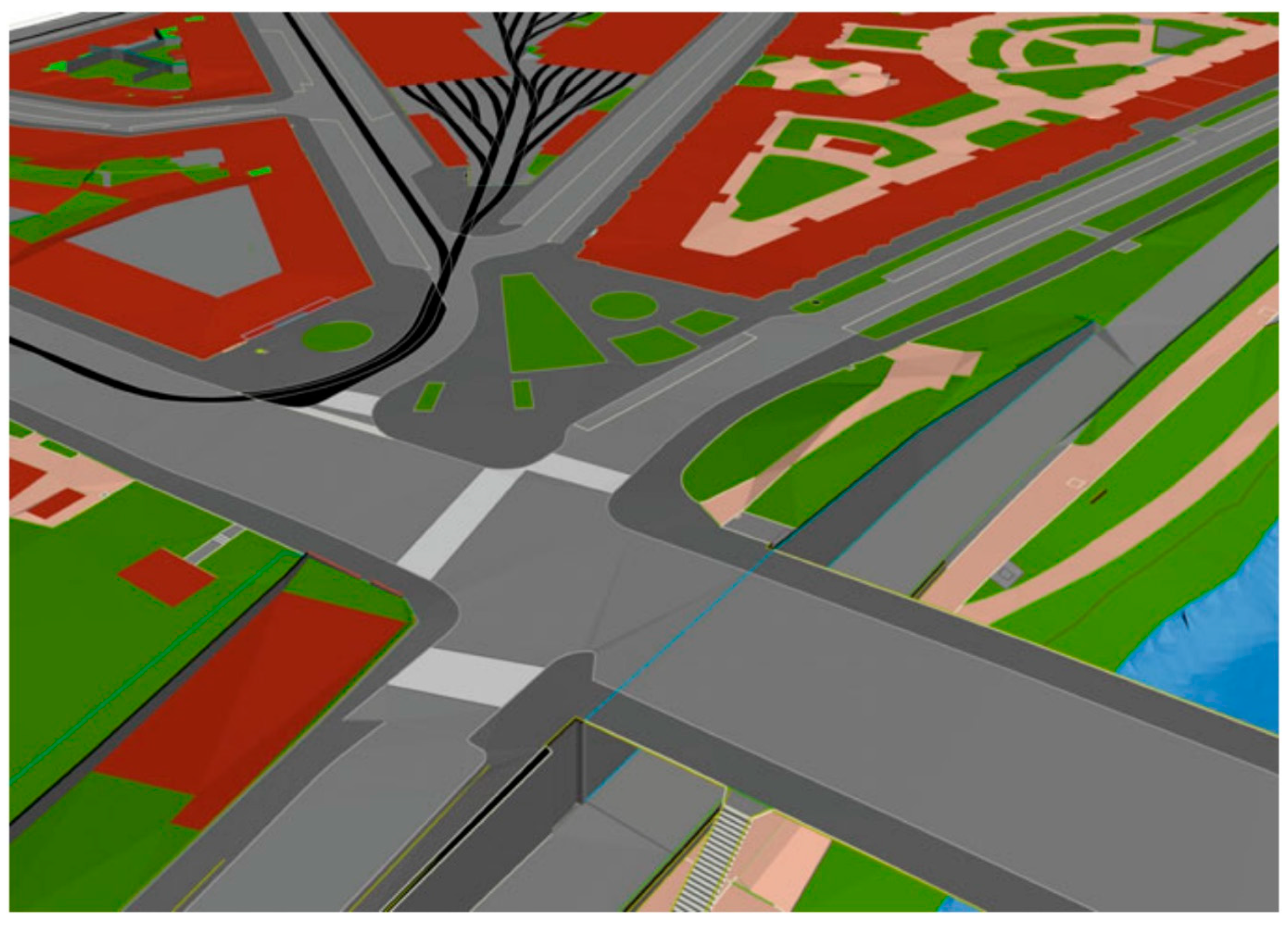
Figure 1. Visualization of land cover objects in the CityGML modules LandUse, Transportation (gray, black) and WaterBody in a study from Vienna [15]; the red objects are virtual surfaces representing building footprints. Source: [15] (p. 529).
Ijgi 14 00328 g001
Figure 3. Workflow of the study.
Ijgi 14 00328 g003
Figure 4. Study area—new Bellevue and Lorensborg neighborhoods of Malmö municipality, southern Sweden.
Ijgi 14 00328 g004
Figure 5. UML diagram of the LandUse module in 3CIM ver. 2.0 with two classes added in the 3CIM ADE: LandCover and LandCoverClosureSurface.
Ijgi 14 00328 g005
Figure 6. The relationship between data reduction in the ALS point cloud (indicating the proportion of points removed from the point cloud when creating the TIN model) and the total vertical uncertainty (Equation (1)). In this test, the land cover boundaries were used as break geometries.
Ijgi 14 00328 g006
Figure 7. Data in the CityGML/3CIM modules to the left where LandCoverClosureSurface represents building footprints (note that the retaining walls in the CityFurniture module are not visible in 2D). This data was merged to generate the 3D LC partition to the right. The LC data is classified at level 3 according to the national specification land cover classes (NS LC).
Ijgi 14 00328 g007
Figure 8. The 3D LC partition classified at level 4 according to the code lists for land cover created in the 3CIM project as an extension of the three levels in the national specification land cover classes (NS LC).
Ijgi 14 00328 g008
Figure 9. Three-dimensional visualization in LOD2 of a part of the study area in Unreal Engine with buildings, trees and walls added to the land cover data for a more realistic visualization. In the upper right corner, the attribute values of the selected road (highlighted with an orange boundary) are shown.
Ijgi 14 00328 g009
Figure 10. Three-dimensional visualization of a pedestrian/biking path with vertical retaining walls. The steep paved path up to the higher level should be steps, but they are not modeled in the study.
Ijgi 14 00328 g010
Table 1. Datasets used to create the land cover data in the study. For the east part of the area, we used data from the CityGML/3CIM modules Buildings and Transportation from 3CIM ver. 1.0 test data [16]. For the remaining area and modules, we used the datasets described in the table.
DataDescriptionAccuracy/ResolutionObservation Year
OrthophotoFrom Malmö municipalitySpatial resolution: 8 cm2018
Terrestrial photosPhotos of the ground surface materials of the inner yards of Bellevuegården (SW part of the study area).cm level2023
2D base mapMunicipality base map representing roads, pavements, parks, etc.Positional accuracy: 10 cmLast update 2023
3D building dataBuilding footprints from 3CIM test area [16] and from City of Malmö’s 3D modelLOD2.1 (according to definition in [53])2022
Transportation dataMajor road polygons were derived from 3CIM test data [16] and the base map from City of Malmö. Minor streets and biking/walking paths were digitized manually based on the city’s orthophoto.Positional accuracy:
Major roads, 10 cm
Walking paths, around 10 cm
Major roads: 2022
Minor roads, biking/walking paths 2018 (as the orthophoto)
ALS point cloudAirborne laser scanning (ALS) data ordered by City of Malmö.Point density: 35–40 points/m2
Vertical accuracy: 5–10 cm
2022
Table 2. The mapping of land cover classes to CityGML modules used in the study.
Land Cover ClassCityGML Module
asphaltTransportation
sett (paving)Transportation
cobblestoneTransportation
grassVegetation
bushesVegetation
poolWaterBody
pondWaterBody
concreteLandUse
natural stoneLandUse
gravel bedLandUse
excavated landLandUse
artificial turfLandUse
rubber surfaceLandUse
paving stoneLandUse
Disclaimer/Publisher’s Note: The statements, opinions and data contained in all publications are solely those of the individual author(s) and contributor(s) and not of MDPI and/or the editor(s). MDPI and/or the editor(s) disclaim responsibility for any injury to people or property resulting from any ideas, methods, instructions or products referred to in the content.