Multi-Channel Spatio-Temporal Data Fusion of ‘Big’ and ‘Small’ Network Data Using Transformer Networks

Abstract

The integration of heterogeneous spatio-temporal datasets presents a critical challenge in geospatial data science, particularly when combining large-scale, passively collected “big” data with precise but sparse “small” data. In this study, we propose a novel framework—Multi-Channel Spatio-Temporal Data Fusion (MCST-DF)—that leverages transformer-based deep learning to fuse these data sources for accurate network flow estimation. Our approach introduces a Residual Spatio-Temporal Transformer Network (RSTTNet), equipped with a layered attention mechanism and multi-scale embedding architecture to capture both local and global dependencies across space and time. We evaluate the framework using real-world mobile sensing and loop detector data from the London road network, demonstrating over 89% prediction accuracy and outperforming several benchmark deep learning models. This work provides a generalisable solution for spatio-temporal fusion of diverse geospatial data sources and has direct relevance to smart mobility, urban infrastructure monitoring, and the development of spatially informed AI systems.

1. Introduction

In the era of ubiquitous computing and digital sensing, the explosive growth of data has transformed how we understand and manage complex systems across a wide range of domains. This transformation is largely driven by the rise of big data: large-scale, high-frequency, and passively collected datasets that offer unprecedented coverage and granularity across both space and time. In contrast, small data refers to datasets that are actively and deliberately collected, typically through precise measurement instruments or manual surveys. While small data is usually of high accuracy and reliability, it tends to be limited in volume and spatial extent due to high acquisition and maintenance costs.

These two types of data—big and small—offer complementary strengths but also pose distinct challenges for analysis and integration. Big data provides wide spatial and temporal coverage, often enabling continuous monitoring at low marginal cost. However, it is inherently noisy and incomplete, frequently capturing only partial observations of the underlying phenomena. Small data, on the other hand, offers ground-truth measurements with high precision, but is often sparsely distributed in space and time. The challenge, therefore, is how to combine the broad, low-fidelity coverage of big data with the sparse but high-fidelity accuracy of small data to reconstruct true spatio-temporal patterns at scale.

Addressing this problem is critical for improving modelling, monitoring, and decision-making across a wide range of networked systems, from infrastructure management to environmental monitoring and social dynamics analysis. However, fusing big and small data streams is not straightforward. Existing approaches often rely on extrapolating from small datasets or smoothing noisy big data, but they typically fail to fully exploit the complementary strengths of both [1]. This motivates the development of a new data fusion paradigm capable of intelligently integrating heterogeneous data sources while addressing three key challenges:

• Mismatch: Traditional time series forecasting methods often assume access to large volumes of accurate data. In practice, however, we are often confronted with an abundance of imprecise, passively collected data combined with a small amount of highly accurate but sparsely distributed observations. This mismatch introduces unique challenges for effective and robust data fusion.
• Sparsity: In real-world systems, high-precision small data is often spatially and temporally sparse due to practical limitations in data collection. This restricted coverage makes it difficult to infer complete system-wide patterns, requiring advanced integration techniques that can effectively leverage limited but high-quality observations.
• Heterogeneity: Although big and small data may reflect similar underlying phenomena, differences in collection methods—such as sampling frequency, resolution, and measurement context—result in heterogeneous data structures. This heterogeneity complicates fusion, as traditional methods often assume homogeneous datasets. A robust integration framework must be capable of learning from diverse, complementary data sources while preserving their unique contributions.

To address these challenges, we propose the Multi-Channel Spatio-Temporal Data Fusion (MCST-DF) framework. This framework utilises spatio-temporal transformer networks to model complex dynamics and effectively mitigate the mismatch between big and small data sources. A layered attention network enables multi-channel spatio-temporal feature embedding, supporting robust integration across heterogeneous inputs. Furthermore, a transformer-based approach is employed to optimise the use of sparse, highly accurate data, enhancing adaptability to incomplete datasets. Empirical tests using real-world network data demonstrate significant improvements in fusion accuracy compared to traditional methods, validating the effectiveness of the proposed MCST-DF framework. To the best of our knowledge, this is the first study focused on addressing the complex challenge of fusing big and small spatio-temporal data across networked systems. The main contributions of this paper are summarised as follows:

• We formalise the problem of fusing network-wide big and small spatio-temporal data for improved prediction and reconstruction.
• We propose the Multi-Channel Spatio-Temporal Data Fusion (MCST-DF) framework and introduce the Residual Spatio-Temporal Transformer Network (RSTTNet) to address the fusion challenge.
• We conduct extensive experiments under a zero-shot setting using a large-scale network dataset, providing a comprehensive visual and quantitative evaluation of the framework’s performance. In this context, the zero-shot setting refers to evaluating model performance on road segments that were completely unseen during training, thereby testing the model’s ability to generalise to new, unobserved parts of the network.

The remainder of this paper is organised as follows. Section 2 reviews related work on spatio-temporal data fusion and discusses existing limitations. Section 3 presents the proposed MCST-DF framework in detail. Section 4 describes the empirical evaluation, including the dataset, experimental design, and results. Finally, Section 5 concludes the paper with a summary of findings, discussion of implications, and suggestions for future research.

2. Related Work

Data fusion has been extensively studied across various domains [2,3], including mobility systems [4], neuroimaging [5], and geoengineering [6]. Early methods focused on converting different data sources into a common feature-based representation, treating the transformed data as a unified dataset [7]. However, such approaches have shown limitations in scalability and flexibility, particularly when applied to spatio-temporal systems where data exhibits complex dynamics across both space and time.

In the context of spatio-temporal data fusion, particular attention has been given to the integration of heterogeneous sources, where spatial and temporal characteristics require fusion strategies that go beyond simple handling of missing data [8,9,10]. Traditional missing-data techniques primarily address data incompleteness but are often insufficient when the integration of diverse sources, each with different levels of quality and coverage, is required. These complexities demand more robust and adaptive fusion frameworks, as discussed in recent works on traffic data imputation and heterogeneous spatio-temporal modelling [8,10,11]. The evolution of deep learning has introduced powerful tools to address some of these challenges, enabling models to capture intricate patterns within large-scale, complex datasets [2,12]. However, most conventional deep learning fusion techniques are designed for homogeneous, high-quality data sources, and often fail when attempting to integrate large volumes of noisy, passively collected data with small volumes of precise, actively collected data. This mismatch, together with the sparsity and heterogeneity of real-world spatio-temporal data, presents fundamental challenges not fully addressed by existing methods.

Current approaches to spatio-temporal data fusion generally fall into three main categories [3]:

• DL-output-based fusion: Independent deep learning models are applied separately to spatial and temporal data, with feature-level merging performed afterward [13]. While this approach provides a solid baseline for feature extraction, it often fails to capture the complex interdependencies across space and time, leading to suboptimal integration.
• DL-input-based fusion: Here, different data sources are merged at the input stage, and a unified deep learning model is trained on the combined data [14]. This method captures some interdependencies during training but may introduce significant computational overhead and scalability challenges when handling very large datasets.
• DL-double-stage-based fusion: A more sophisticated approach that fuses data at both the input and output stages, offering improved handling of data complexity through multiple layers of processing [15]. However, this approach often assumes compatibility and uniform coverage across datasets, which limits its applicability in settings characterised by mismatched and incomplete data sources.

Although these methods have shown effectiveness in specific applications, they are fundamentally unsuited for fusing large-scale spatio-temporal data where the “big” and “small” data sources differ sharply in quality, coverage, and structure. Mismatch is a key challenge: integrating abundant but imprecise data with sparse yet highly accurate data requires models that can handle varying levels of uncertainty. For instance, ref. [16] introduced a macro–micro-spatio-temporal network to leverage data at different granularities. While promising, this method relies heavily on precise spatio-temporal alignment, limiting its effectiveness under significant mismatch. Similarly, methods based on embedding techniques or graph structures [11,17] often assume homogeneity across data sources, which constrains their ability to integrate heterogeneous, misaligned datasets. Sparsity presents another major hurdle, where small data is geographically or temporally limited, making it difficult to generalise across large networks. Graph-based methods such as GraphSAGE [18] and cluster-based flow estimation models [19] attempt to infer missing data, but they often fail to fully leverage the precision of sparse, ground-truth observations for network-wide predictions. Heterogeneity complicates integration further, as big and small data sources frequently differ in structure, resolution, and measurement practices. Some hybrid models [20,21] attempt to unify heterogeneous data through embedding strategies, but rigid model structures often struggle to dynamically adapt to highly diverse inputs found in complex networks.

In summary, although considerable progress has been made in spatio-temporal data fusion, existing methods often fall short when confronted with the combined challenges of data mismatch, sparsity, and heterogeneity. Many current frameworks assume homogeneous and well-aligned datasets, and struggle to integrate large volumes of noisy, low-fidelity data with limited but high-quality observations [22,23,24]. These limitations highlight the need for a new approach capable of robustly fusing diverse data sources across complex networks while preserving both accuracy and scalability. In response, we propose the Multi-Channel Spatio-Temporal Data Fusion (MCST-DF) framework, specifically designed to integrate heterogeneous datasets, address sparsity, and manage data mismatch effectively. Our framework demonstrates significant potential for improving predictive accuracy and enhancing robustness in large-scale spatio-temporal systems by optimising the fusion of complex, diverse data streams.

3. Preliminaries and Problem Formulation

In this section, we formally define the problem of fusing “big” and “small” network data, providing the foundation for the methodologies and experiments that follow.

Problem Formulation

This study addresses a general challenge: how to effectively integrate heterogeneous big and small data sources to estimate the true underlying flow across complex networks. Mathematically, we seek to develop a function that maps observations from both big and small datasets to an accurate estimation of the true flow. The problem can be formulated as follows:

$$S_{0,0,T}=f\left({\{B_{i,j,t},S_{i,j,t}·I_{i,j,t}\}}_{i=0,j=1,t=0}^{i=3,j=N_i,t=T}\right)$$

(1)

where

• $S_{i,j,t}$ represents the small data for the j-th road in the i-th order neighbourhood at time t;
• $B_{i,j,t}$ represents the big data for the same segment;
• $I_{i,j,t}$ is an indicator function that denotes the availability of small data for each segment at each time point (1 if available, 0 otherwise);
• $N_i$ is the number of roads in the i-th order neighbourhood, of which the i-th order neighbourhood includes all segments reachable from the target segment within i hops; the 0-th order neighbourhood consists of the target segment itself.

The function f predicts flow on the target road at time T using both big data and any small data available from the road and its neighbours up to the third order. Each segment of the road and its neighbours are identified by their order in the neighbourhood (i) and an index (j), with $i=0$ representing the target road itself.

To simplify the flow representation across the network, we use the notation $F_{0,0,t}$ to denote the total flow, which includes two components: the accurate unknown flow (UF) and the known flow, represented by small data. Our goal is to use both big and small data to infer the unknown flow UF accurately.

The inclusion of data up to the third-order neighbourhood is supported not only by empirical findings from previous work [24,25], which showed that dynamic spatial autocorrelation diminishes significantly beyond the third order, but also by established spatial statistics theory. In particular, Anselin’s work on local indicators of spatial association (LISA) demonstrates that spatial dependencies typically decay rapidly with distance, and higher-order neighbourhoods often contribute negligible correlation [26]. Therefore, limiting the neighbourhood to the third order is both empirically and theoretically justified for capturing significant spatial dependencies while ensuring computational efficiency.

However, if there are no available small data within the third-order neighbourhood, the accuracy of the estimation for the unknown flow may diminish, as our model relies on integrating small data alongside big data to enhance precision. In cases where small data is unavailable within this threshold, alternate small data modelling methods are employed to approximate the missing small data impact.

To address this complexity, we propose a Multi-Channel Spatio-Temporal Data Fusion (MCST-DF) framework that allows us to derive the unknown flow by optimally combining the information from both big and small data sources. We will introduce the MCST-DF framework in detail in the next section.

4. Methodology

In this section, we present the Multi-Channel Spatio-Temporal Data Fusion (MCST-DF) framework. First, we outline the general framework, providing a high-level understanding of the approach. Then, we introduce the embedding network designed specifically for extracting spatio-temporal features effectively. Next, we elaborate on the RSTTNet, which is pivotal for modelling network-based spatio-temporal dependencies. Lastly, we discuss the optimisation objective, which guides the training process to achieve the desired performance.

4.1. Multi-Channel Spatio-Temporal Data Fusion Framework

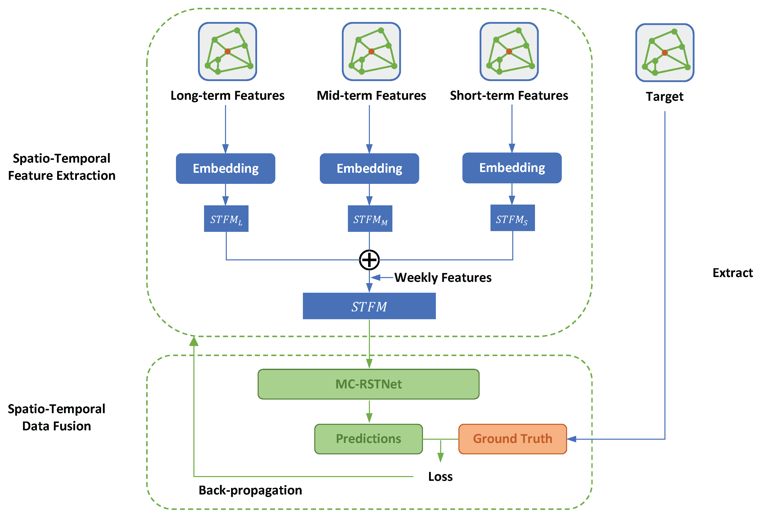
To address the problem of data fusion between network-wide “big” and “small” flow data, we propose the Multi-Channel Spatio-Temporal Data Fusion (MCST-DF) framework, which consists of two modules, as shown in Figure 1. Our MCST-DF framework extends beyond standard Transformer architectures by introducing multi-scale temporal channels and hierarchical neighbourhood modelling. Specifically, we design separate temporal channels (long-term, mid-term, short-term) to capture dynamics at varying time scales, and a layered attention mechanism to process different neighbourhood orders (0th–3rd) independently. These innovations enable the model to learn from noisy but comprehensive big data while effectively integrating sparse yet high-precision small data. In our framework, the term multi-channel explicitly denotes the construction of separate feature channels in both temporal and spatial dimensions. Temporally, we divide historical data into long-term, mid-term, and short-term channels. Spatially, we construct channels for the target road and its 1st- to 3rd-order neighbours. This design enables the model to capture multi-scale dependencies within each data source. Meanwhile, the multi-scale aspect of our framework refers to the combination of heterogeneous big and small datasets.

Multi-Channel Spatio-Temporal Feature Extraction. The input data is processed and segmented into three distinct temporal features: long-term, mid-term, and short-term features. This division enables the model to capture patterns and dependencies at various temporal resolutions, thereby enhancing its ability to comprehend complex temporal dynamics. Each set of temporal features is passed through an embedding layer. The embedding layers transform these raw features into dense, lower-dimensional representations that encapsulate the essential spatio-temporal information. This transformation results in the creation of Spatio-Temporal Feature Maps (STFM), denoted as $STF{M}_L$, $STF{M}_M$, and $STF{M}_S$ for long-term, mid-term, and short-term features, respectively. The individual Spatio-Temporal Feature Maps are then combined into a unified feature representation. This process integrates the diverse temporal information, allowing the model to utilise the comprehensive spatio-temporal context provided by all three feature sets.

Spatio-temporal Data Fusion. The concatenated spatio-temporal feature map is fed into the Residual Spatio-Temporal Transformer Network (RSTTNet), which is specifically designed to handle multi-channel spatio-temporal data.

The predicted flows generated by the RSTTNet are compared against the ground-truth flow values to compute the MSE loss. The whole framework is trained end-to-end using backpropagation, where the loss gradients are propagated back through the network to optimise the model parameters.

4.2. Multi-Channel Spatio-Temporal Feature Extraction

4.2.1. Multi-Channel Spatio-Temporal Feature Construction

To better capture spatio-temporal information on the network and make full use of both big data and small data for improved data fusion, we need to construct reasonable spatio-temporal features. Our approach focuses on two key aspects: multi-channel temporal feature construction and multi-channel spatial feature construction.

Temporal Features. To accurately capture the temporal dynamics in network data, we utilise three months of historical data. The rationale behind selecting a three-month period is rooted in the need to encompass various temporal patterns, such as short-term, mid-term, and long-term trends, each of which serves as a distinct channel of temporal information. This time frame is long enough to observe recurring events and trends, which are crucial for making accurate fusion of short-term flow. For instance, certain flow patterns may only emerge over longer periods, such as long-term variations, while mid-term and short-term patterns capture regular commuting behaviours.

In addition, we introduce a weekly feature, where each day of the week is treated as a separate entity. For instance, Monday’s patterns are captured distinctly from Tuesday’s, and so forth for each day through to Sunday. This approach allows us to create an additional channel specifically for daily variances. When making predictions for a particular day (e.g., Monday), the corresponding weight for that day is selectively applied to enhance the model’s accuracy. By incorporating this weekly feature, we add a nuanced temporal dimension that better reflects the unique daily patterns within weekly cycles, further enriching our temporal representation of network data.

Temporal Multi-channel Mechanism. The multi-channel mechanism refers to the process of learning a model from historical data at multiple scales to predict accurate flow. By selecting historical data at varying scales, such as time slices from a few days, a week, or several months, the model can capture a broader range of features and thus enhance its performance. This approach takes advantage of different temporal dimensions to improve the accuracy of predicted flows. Specifically, the features corresponding to long-term, mid-term, and short-term data are denoted as $F_L$, $F_M$, and $F_D$ respectively.

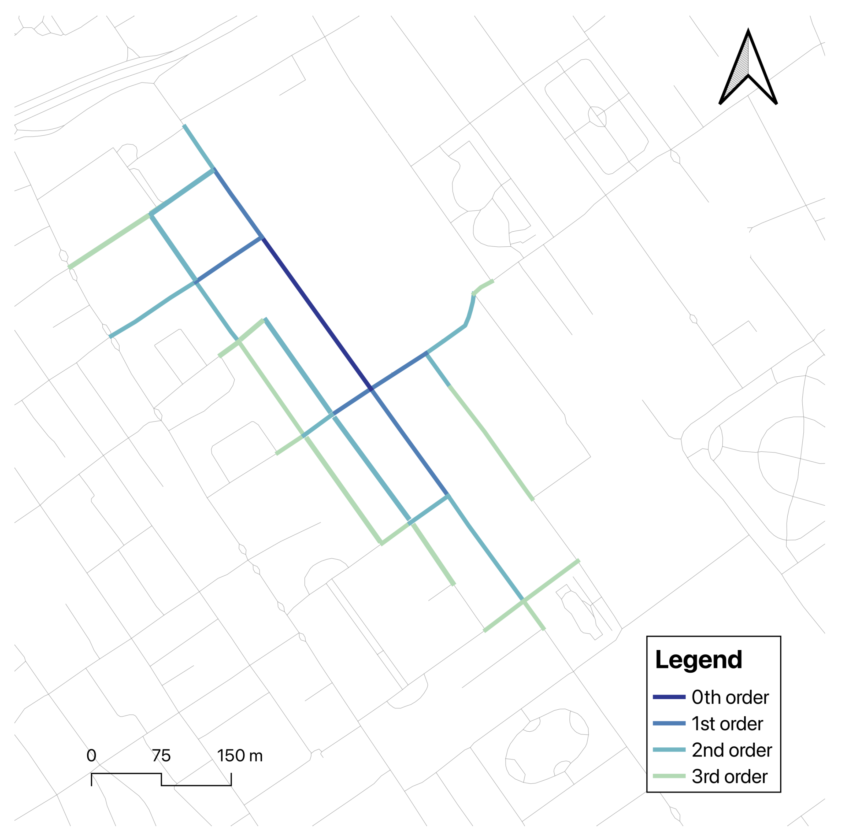
Spatial Features. In the domain of network analysis, spatial features are pivotal for comprehending the impact of neighbouring areas on a specific location. To construct these spatial features, we extract 0th- to 3rd-order neighbours, effectively creating a sub-graph of the entire network as depicted in Figure 2. This approach entails not only analyzing a location’s immediate neighbours but also considering the neighbours of these neighbours up to three levels deep. The rationale behind this methodology is that network conditions at a specific site are frequently influenced by a wider area beyond the immediate vicinity. By incorporating 0th- to 3rd-order neighbours into our analysis, we can capture more intricate spatial interactions and dependencies, thereby providing a more holistic understanding of the network dynamics. This comprehensive approach enables us to uncover patterns and relationships that would be overlooked if only immediate neighbours were considered.

Spatial Multi-channel Mechanism. Similar to the temporal multi-channel mechanism, the spatial multi-channel mechanism handles spatial features by treating different orders of neighbouring roads as separate channels. Specifically, the 0th-order neighbour (the road itself), as well as the 1st-, 2nd-, and 3rd-order neighbours, are each treated as distinct channels of spatial information. This multi-channel approach enables the model to capture spatial dependencies at various scales. For example, the 1st-order neighbours reflect the immediate surrounding network conditions, while higher-order neighbours provide information about more distant but still relevant areas in the network. By learning spatial patterns across these different channels, the model can account for both local and more global network interactions, enhancing its ability to predict flows with greater accuracy. This layered structure captures a broader and more detailed view of the network, much like how the temporal multi-channel mechanism enriches the temporal dynamics.

To enhance the model’s utilisation of spatio-temporal data, it is imperative to preprocess the data instead of directly passing raw, varying-length sequences to the subsequent layers. This preprocessing is achieved through the Layered Attention Network (LAN), which systematically organises and embeds the data. Following this, the integrated spatio-temporal feature map is generated, providing a unified representation that captures the intricate spatial and temporal dependencies essential for accurate data fusion. Details on the LAN framework will be discussed in the following section.

4.2.2. Layered Attention Network for Multi-Channel Spatio-Temporal Feature Embedding

The Layered Attention Network (LAN) plays a crucial role in our framework by embedding spatial and temporal features into a comprehensive feature map. This module is essential for capturing the correlations and patterns across different time scales, which significantly enhances the model’s predictive capabilities.

In dynamic networks, the propagation of information often varies based on the proximity and connectivity of the network. Therefore, segmenting information according to different orders of neighbours (0th, 1st, 2nd, and 3rd) allows the model to more accurately capture the hierarchical and localised influences within the network. This segmentation is critical because network patterns are often influenced by both immediate and distant road segments, necessitating a structured approach to information integration.

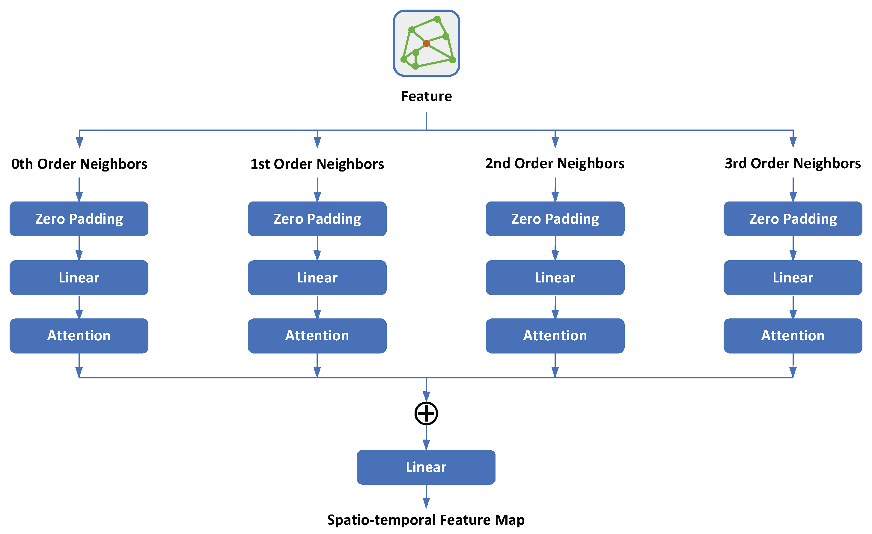
As discussed previously, we have obtained the long-term, mid-term, and short-term features. By processing these features through the embedding network, we obtain the corresponding embedding network feature map. The structure of the embedding network is illustrated in Figure 3. In this architecture, the feature is passed through multiple layers that handle different orders of neighbours (0th, 1st, 2nd, and 3rd). Each layer consists of the following components:

• Zero Padding: To maintain the spatial dimensions, zero padding is applied to the input features.
• Linear Layer: A linear layer is applied to project the input features into a higher dimensional space.
• Attention Mechanism: An attention mechanism is employed to focus on the most relevant parts of the input features.

One of the significant advantages of the LAN lies in its ability to flexibly handle the varying numbers of neighbours in networks. Traditional Graph Convolutional Networks (GCN) face complexities due to the inconsistent number of neighbours for different roads [27]. LAN addresses this issue through the use of padding techniques, ensuring that the number of neighbours in each layer remains consistent. This consistency in input dimensions allows the model to process nodes with diverse connectivity patterns seamlessly, avoiding the need for complex sampling or pooling operations. Furthermore, the attention mechanism allows the model to weigh the importance of different data points, making it particularly effective in scenarios with heterogeneous data sources such as GPS and ATC data. This design specifically addresses the spatial heterogeneity between big data’s wide coverage and small data’s localised precision, allowing the model to assign appropriate importance to each neighbourhood based on its data quality and availability.

Moreover, traditional GCN-based methods model the entire network as a single graph, leading to substantial computational overhead and exacerbating the Zero-inflated problem [28] in small data scenarios. To mitigate these issues, we employ LAN to process information from different hierarchical levels of neighbours. By categorising neighbours into 0–3 hop layers and processing each layer independently, LAN effectively captures the hierarchical relationships among neighbours. The linear and attention mechanisms in each layer focus on extracting information specific to that tier, thereby preventing the blending of information that typically occurs in GCNs. This hierarchical processing enhances the model’s ability to accurately represent and leverage the unique contributions of each layer, thus improving overall predictive performance.

After processing through these layers, the outputs from each order of neighbours are concatenated and passed through a final linear layer to generate the spatio-temporal feature map, which captures both spatial and temporal dependencies. This spatio-temporal feature map is crucial as it serves as a unified representation that integrates information across different scales and locations. By capturing these dependencies, the feature map enables the model to understand complex patterns within the data.

4.2.3. Spatio-Temporal Feature Map

In Figure 1, the feature extraction part includes three sub-models, which respectively generate the long-term, mid-term, and recent spatio-temporal feature maps. The three sub-models shared an identical structure: the embedding network. This embedding network is specifically designed for the geographically-based road network, where neighbourhood relationships are derived from the spatial topology of the transport network, integrating both the geographical locations and the connectivity of road segments. The integration of spatial and temporal features on the feature map allows for the simultaneous modelling of correlations in both space and time. Although many existing works opt for a simple summation-based approach to merge feature maps [27,29], this method tends to overlook the multi-channel nature of data and can result in significant information loss. Instead, we employ a parameter-based method to concatenate the three feature maps: long-term, mid-term, and recent features (denoted as $STF{M}_L$, $STF{M}_M$, and $STF{M}_S$, respectively). Equation (2) defines this method:

$$STFM=STF{M}_L·W_L\oplus STF{M}_M·W_M\oplus STF{M}_S·W_S$$

(2)

where $STFM$ represents the combined spatio-temporal feature map, $STF{M}_M$, $STF{M}_L$, and $STF{M}_S$ denote the long-term, mid-term, and short-term spatio-temporal feature maps, respectively, and $W_L$, $W_M$, and $W_S$ are trainable scalar weights corresponding to the long-term, mid-term, and short-term spatio-temporal feature maps, respectively. These parameters are optimised during training via backpropagation to automatically adjust the contribution of each temporal scale to the final prediction.

The resulting spatio-temporal feature map captures comprehensive spatio-temporal patterns by effectively combining information from different time scales. This combined feature map is then fed into the next module, RSTTNet, to further enhance the model’s predictive accuracy and capability.

4.3. RSTTNet for Network-Based Spatio-Temporal Data Fusion

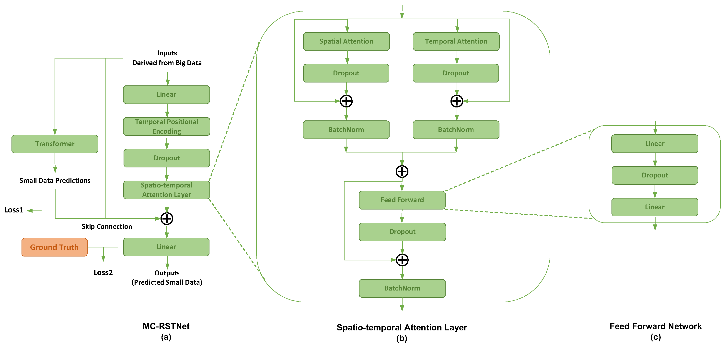
The Residual Spatio-Temporal Transformer Network (RSTTNet) is designed to capture and model spatio-temporal dependencies in network-based data. The architecture of RSTTNet, as illustrated in Figure 4, with Figure 4a showing the overall architecture, and Figure 4b,c presenting the framework of the spatio-temporal attention layer and its feed-forward network, begins with an initial linear transformation applied to the inputs. This is followed by a temporal positional encoding. This encoding helps the network understand the temporal aspects of the data. After the temporal positional encoding, a dropout layer is applied to prevent overfitting by randomly setting a fraction of input units to zero at each update during training.

4.3.1. Small Data Modelling for Effective Data Utilisation

To solve the problem of small data sparsity, which is a core issue in data fusion as opposed to traditional time series prediction problems, it is crucial to address the scarcity of real label information. To effectively utilise the limited available labels, we adopt a specific modelling approach. Initially, we use the few available real labels to model the small data, enabling us to generate relatively accurate small data. This approach partially addresses the problem of insufficient small data.

The upper part of Figure 4a illustrates the transformer module used for small data modelling. The input consists of big data, and the output is small data. The predicted small data are compared with the ground truth small data by computing the Mean Squared Error (MSE) loss to ensure accuracy. Although the predicted small data is relatively accurate, it is not sufficiently precise. Consequently, the relatively accurate small data predicted by the transformer module, along with the big data, is fed into the subsequent model to enhance the final prediction accuracy of the small data. This process can be understood as the subsequent model learning the residuals between the ground-truth small data and the small data predicted by the transformer model. By leveraging this residual learning approach, we aim to refine the predicted flows and address the challenges posed by the limited availability of label information in data fusion tasks. This residual learning mechanism helps bridge the gap in data quality, ensuring the model can accurately estimate flows even when small data is unavailable or sparse, thus directly tackling the mismatch challenge between heterogeneous inputs.

4.3.2. Temporal Positional Encoding

Temporal positional encoding is a fundamental technique in transformer models, designed to inject information about the sequence order of the input data. This method allows the model to distinguish between different positions within a sequence, an ability that is critical for processing temporal data effectively.

The core idea of temporal positional encoding is to generate unique positional vectors for each position in the sequence. These vectors are then added to the input embeddings, thus incorporating temporal information. The encoding vectors are constructed using sine and cosine functions of different frequencies. This approach ensures that the positional encodings are smoothly varying and distinct across dimensions.

The positional encoding vector $\mathrm{PE}(pos,2i)$ for a given position $pos$ and even dimension $2i$ is defined as follows:

$$\mathrm{PE}(pos,2i)=sin\left({\displaystyle \frac{pos}{{10000}^{2i/d}}}\right)$$

(3)

For odd dimensions $2i+1$, the positional encoding vector is given by the following:

$$\mathrm{PE}(pos,2i+1)=cos\left({\displaystyle \frac{pos}{{10000}^{2i/d}}}\right)$$

(4)

where d represents the dimensionality of the input embeddings. The use of sine and cosine functions at varying frequencies allows the encoding to capture both short-term and long-term dependencies in the data. Specifically, the division term ${10000}^{2i/d}$ ensures that the wavelengths form a geometric progression, providing a range of periodicities suitable for different positional dependencies.

By adding these positional encodings to the input embeddings, the transformer model can leverage the temporal information effectively, enabling it to process and understand sequential data such as time series, language, and more. This mechanism is essential for tasks that require an understanding of the order and structure within the input data.

4.3.3. Spatio-Temporal Attention Layer

The core component of RSTTNet is the spatial–temporal attention layer, depicted in Figure 4b. This layer is responsible for capturing both spatial and temporal dependencies in the data. It consists of two main sub-layers: the spatial attention layer and the temporal attention layer. Each sub-layer includes a dropout mechanism to improve generalisation and a batch normalisation (BatchNorm) layer to stabilise and accelerate training by normalising the input features.

Temporal Attention Layer. Temporal attention is designed to model the temporal dependencies. It computes attention weights across the temporal dimension for each joint. Given a sequence of embeddings $\mathbf{X}\in {\mathbb{R}}^{B\times T\times D}$ where B is the batch size, T is the sequence length, and D is the embedding dimension; the temporal attention layer performs the following operations:

$$\begin{array}{cc}\hfill {\mathbf{Q}}_{h,i}& ={\mathbf{X}}_i{\mathbf{W}}_{h,i}^Q\hfill \end{array}$$

(5)

$$\begin{array}{cc}\hfill {\mathbf{K}}_{h,i}& ={\mathbf{X}}_i{\mathbf{W}}_{h,i}^K\hfill \end{array}$$

(6)

$$\begin{array}{cc}\hfill {\mathbf{V}}_{h,i}& ={\mathbf{X}}_i{\mathbf{W}}_{h,i}^V\hfill \end{array}$$

(7)

$$\begin{array}{cc}\hfill {\mathbf{A}}_{h,i}& =\mathrm{Softmax}\left({\displaystyle \frac{{\mathbf{Q}}_{h,i}{\mathbf{K}}_{h,i}^T}{\sqrt{d_k}}}+\mathbf{M}\right)\hfill \end{array}$$

(8)

$$\begin{array}{cc}\hfill {\mathbf{O}}_{h,i}& ={\mathbf{A}}_{h,i}{\mathbf{V}}_{h,i}\hfill \end{array}$$

(9)

where ${\mathbf{W}}_{h,i}^Q,{\mathbf{W}}_{h,i}^K,{\mathbf{W}}_{h,i}^V$ are the learned weight matrices for the i-th joint and h-th attention head, $d_k$ is the dimension of the keys (and queries), and $\mathbf{M}$ is a mask applied to ensure causality (only attending to past time steps).

The outputs from all heads are concatenated and projected back to the original embedding dimension:

$$\begin{array}{cc}\hfill {\mathbf{O}}_h& =\mathrm{Concat}({\mathbf{O}}_{h,1},{\mathbf{O}}_{h,2},\dots ,{\mathbf{O}}_{h,N})\hfill \end{array}$$

(10)

$$\begin{array}{cc}\hfill \mathbf{Z}& ={\mathbf{O}}_h{\mathbf{W}}^O\hfill \end{array}$$

(11)

where ${\mathbf{W}}^O$ is the projection matrix of the output.

Spatial Attention Layer. Spatial attention focuses on capturing the spatial relationships in the data across different joints. Given the same sequence of embeddings $\mathbf{X}$, the spatial attention layer performs the following operations:

$$\begin{array}{cc}\hfill {\mathbf{Q}}_h& =\mathbf{X}{\mathbf{W}}_h^Q\hfill \end{array}$$

(12)

$$\begin{array}{cc}\hfill {\mathbf{K}}_h& =\mathbf{X}{\mathbf{W}}_h^K\hfill \end{array}$$

(13)

$$\begin{array}{cc}\hfill {\mathbf{V}}_h& =\mathbf{X}{\mathbf{W}}_h^V\hfill \end{array}$$

(14)

$$\begin{array}{cc}\hfill {\mathbf{A}}_h& =\mathrm{Softmax}\left({\displaystyle \frac{{\mathbf{Q}}_h{\mathbf{K}}_h^T}{\sqrt{d_k}}}\right)\hfill \end{array}$$

(15)

$$\begin{array}{cc}\hfill {\mathbf{O}}_h& ={\mathbf{A}}_h{\mathbf{V}}_h\hfill \end{array}$$

(16)

Again, the outputs from all heads are concatenated and projected back:

$$\begin{array}{cc}\hfill {\mathbf{O}}_s& =\mathrm{Concat}({\mathbf{O}}_{s,1},{\mathbf{O}}_{s,2},\dots ,{\mathbf{O}}_{s,N})\hfill \end{array}$$

(17)

$$\begin{array}{cc}\hfill \mathbf{Y}& ={\mathbf{O}}_s{\mathbf{W}}^O\hfill \end{array}$$

(18)

Aggregation. Lastly, the combined output from the temporal and spatial attention layers is passed through a feed-forward network (FFN) to produce the final output, as shown in Figure 4c. The feed-forward network consists of a series of linear transformations interspersed with dropout layers to further refine the features extracted by the attention mechanisms:

$$\begin{array}{cc}\hfill \mathbf{F}& =\mathrm{ReLU}(\mathbf{Z}{\mathbf{W}}_1+{\mathbf{b}}_1)\hfill \end{array}$$

(19)

$$\begin{array}{cc}\hfill \mathbf{G}& =\mathbf{F}{\mathbf{W}}_2+{\mathbf{b}}_2\hfill \end{array}$$

(20)

where ${\mathbf{W}}_1,{\mathbf{W}}_2$ are the weights of the FFN, and ${\mathbf{b}}_1,{\mathbf{b}}_2$ are the biases. Dropout and batch normalisation are applied as needed to improve generalisation and training stability. The spatial–temporal attention mechanism thus allows the model to effectively capture both temporal and spatial dependencies in the data, enabling more accurate data fusion. The outputs from the feed-forward network are combined and normalised using BatchNorm, as shown in Figure 4b.

4.3.4. Residual Connection

Residual learning [30] has proven to be a powerful technique for training deep neural networks by facilitating gradient flow and allowing the model to learn meaningful features more easily. In our approach, the output of the spatio-temporal attention layer and the output of the transformer module are added to the original input through a residual connection. This skip connection helps mitigate the vanishing gradient problem and enables the construction of deeper networks.

Lastly, the processed features pass through another linear layer to produce the final output. This architecture allows RSTTNet to effectively model complex spatio-temporal dependencies, making it well-suited for tasks involving network-based data where both spatial and temporal dynamics are critical.

4.4. Optimisation Objective

In the training process, the objective is to optimise the function f by minimising a combined loss, which includes three components: the MSE loss between the output of the transformer module and actual flows, the MSE loss between the model’s final predicted output and actual flows, and an L2 regularisation loss.

Firstly, the MSE loss between the output of the transformer module and actual flows ($LOS{S}_1$) is defined as follows:

$$LOS{S}_1={\displaystyle \frac{1}{N}}\sum _{t=1}^N{(S_t-{\widehat{S}}_{trans,t})}^2$$

(21)

where N is the number of observations in the training set, $S_t$ represents the actual observed small data at time t, and ${\widehat{S}}_{trans,t}$ represents the predicted output from the transformer module at time t.

Secondly, the MSE loss between the model’s final predicted output and actual flows ($LOS{S}_2$) is defined as follows:

$$LOS{S}_2={\displaystyle \frac{1}{N}}\sum _{t=1}^N{(S_t-{\widehat{S}}_t)}^2$$

(22)

where ${\widehat{S}}_t$ represents the model’s final predicted output for the target road at time t.

Thirdly, the L2 regularisation loss ($L{2}_{reg}$) is included to prevent overfitting by penalising large weights in the model. This regularisation term is defined as follows:

$$L{2}_{reg}={∥\theta ∥}_2^2$$

(23)

where $\theta$ denotes the model parameters.

The final combined loss function is given by the following:

$$LOSS=LOS{S}_1+LOS{S}_2+{\lambda }_{L2}·L{2}_{reg}$$

(24)

In this equation, ${\lambda }_{L2}$ is the weight for the L2 regularisation loss, set to 0.01. By minimising this combined loss, the training process ensures that the model accurately predicts flows while maintaining robustness and preventing overfitting through regularisation. This comprehensive approach optimises the model’s performance by integrating both the predicted outputs and the regularisation term into the training objective.

Our algorithm uses backpropagation to update network parameters and train the model. By calculating the gradient of the loss function with respect to the network’s parameters, backpropagation allows us to make iterative adjustments to minimise the loss and improve the model’s performance. This end-to-end optimisation approach ensures that all components of the model are tuned simultaneously to achieve the best possible predictive accuracy. The detailed pseudocode for our method is provided in Algorithm 1.

Algorithm 1 Multi-Channel Spatio-Temporal Data Fusion (MCST-DF) Framework

1: Input: Input data D  2: Output: Predicted results  3: for each training epoch do  4:    for each data sample d in D do  5:      Spatio-temporal Feature Extraction  6:      for each road in d do  7:         Extract 0th to 3rd order neighbours to construct spatial features  8:      end for  9:      Extract temporal features from three months of historical data 10:     Segment spatio-temporal features into long-term features $F_L$, mid-term features $F_M$, and recent features $F_S$ 11:     Construct multi-channel features $F_L$, $F_M$, and $F_S$ for different temporal scales 12:     Generate long-term, mid-term, and recent feature maps $STF{M}_L$, $STF{M}_M$, and $STF{M}_S$ using Layered Attention Network (LAN) 13:     Combine feature maps using Equation (2) to obtain $STFM$ 14:     RSTTNet for Network-Based Spatio-temporal Data Fusion 15:     Input $STFM$ into RSTTNet 16:     Apply temporal positional encoding 17:     Pass through spatio-temporal attention layers 18:     Input $STFM$ into transformer module and generate predicted flows 19:     Combine all the information and generate final predicted flows for d 20:     Compute Loss and Update 21:     Compute $LOS{S}_1$ by comparing the transformer’s predicted output with the actual flows 22:     Compute $LOS{S}_2$ by comparing the model’s final predicted output with the actual flows 23:     Compute $L{2}_{reg}$ as the L2 regularisation term 24:     Compute the total loss: $LOSS=LOS{S}_1+LOS{S}_2+{\lambda }_{L2}·L{2}_{reg}$ using Equation (24) 25:     Minimise the accumulated loss using backpropagation 26:     Update model parameters iteratively to improve predictive accuracy 27:    end for 28: end for

5. Experiment and Analysis

In this section, we present comprehensive experiments and analyses to validate the effectiveness of the proposed MCST-DF framework and RSTTNet. We systematically cover the following aspects: datasets utilised in our study, the environment and training settings, the baselines for comparison, and the evaluation metrics employed. Additionally, we explore the experimental results and their analysis, provide visualisations to illustrate key findings, perform sensitivity analysis to assess the robustness of our model and conduct ablation studies to understand the contribution of each component of RSTTNet. By conducting these experiments, we aim to provide a comprehensive evaluation of the proposed methods and demonstrate their superior performance, robustness to parameter variations, and the significance of their individual components. This work focuses on the effective integration of big data and small data. Although we use traffic flow data as an example, our approach is generalisable to other domains.

5.1. Experiment Settings

5.1.1. Dataset Description

In this case study, two primary datasets were used to validate the effectiveness of the proposed MSCT-DF framework and RSTTNet.

First, driving flow data derived from mobile phone applications serves as the proxy for big data. This data, collected with GDPR consent, is compiled from more than 50 mobile phone applications used by UK citizens and visitors, including travel-related and lifestyle applications. The dataset provides a range of valuable indicators, such as device ID, location, time, and speed. Although the device ID is initially linked to an individual and can be tracked over prolonged periods, robust anonymisation techniques, such as ID hashing, are applied to safeguard personal privacy. Furthermore, data handling is conducted in the security computing environment, compiling with ethical standards and legal frameworks to prevent re-identification and misuse. During preprocessing, GPS points are matched to road segments using spatial map-matching algorithms and filtered using techniques embedded within the travel mode detection framework. These include noise reduction and outlier removal to exclude implausible trajectories, such as unrealistic speed jumps or inconsistent travel paths.

A hierarchical segment-based travel mode detection algorithm is adopted to detect comprehensive travel modes from mobile phone data, including car, bus, train, tube, cycle, walk, and stationary [31]. This algorithm integrates a moving-window Support Vector Machine (SVM) with Geographic Information System (GIS) techniques and rule-based methods [32]. According to individuals’ routes and travel modes, driving flow can be generated from mobile phone application datasets with travel mode information. This dataset can provide short-term or hourly sampled flow information for the entire road network, which has 45,572 links in total [33]. These are the “big” data for our case.

Additionally, hourly traffic data from Transport for London is used to represent small data. This data is collected from a set of 296 automatic traffic counters (ATCs). ATCs are magnetic loops embedded in the road that count all motorised vehicle movements passing over the loop. These ATCs were originally deployed to provide a statistically representative flow count at the levels of central, inner, and outer London, as well as at the specific locations where the ATCs were installed. ATC data is temporally aligned with mobile phone flow data by matching timestamps and spatially matched by road segment IDs.

We represent the urban road network as a directed spatial graph, where nodes correspond to major intersections and edges represent individual road segments. The spatial geometry of the network was derived from the Ordnance Survey Integrated Transport Network (ITN), providing a consistent and topologically accurate base map for spatial analysis. High-quality “small” data were obtained from Automatic Traffic Counters (ATC), maintained by Transport for London (TfL). These detectors provide daily aggregated flow counts and have been pre-processed and spatially aligned with the Ordnance Survey road network by the data provider. As such, each ATC record is mapped directly to a specific road segment within the base network. Given their reliability and precision, we treat the ATC flow counts as ground-truth calibration data. These small but authoritative observations form the benchmark against which the fusion model is trained and evaluated.

The sparse and spatially biased distribution of ATC sensors presented a significant challenge for generalising across the entire network. These sensors are predominantly located along major arterial roads and in central areas, resulting in limited calibration coverage for peripheral or lower-volume segments. To address this, our model incorporates spatial attention mechanisms that learn dynamic spatial dependencies beyond local neighbourhoods, enabling effective generalisation to unobserved areas. We further evaluated the model’s generalisability through zero-shot prediction experiments on road segments with no direct ATC observations, demonstrating its capacity to infer plausible flows based solely on contextual information from big data and the learned spatial–temporal structure.

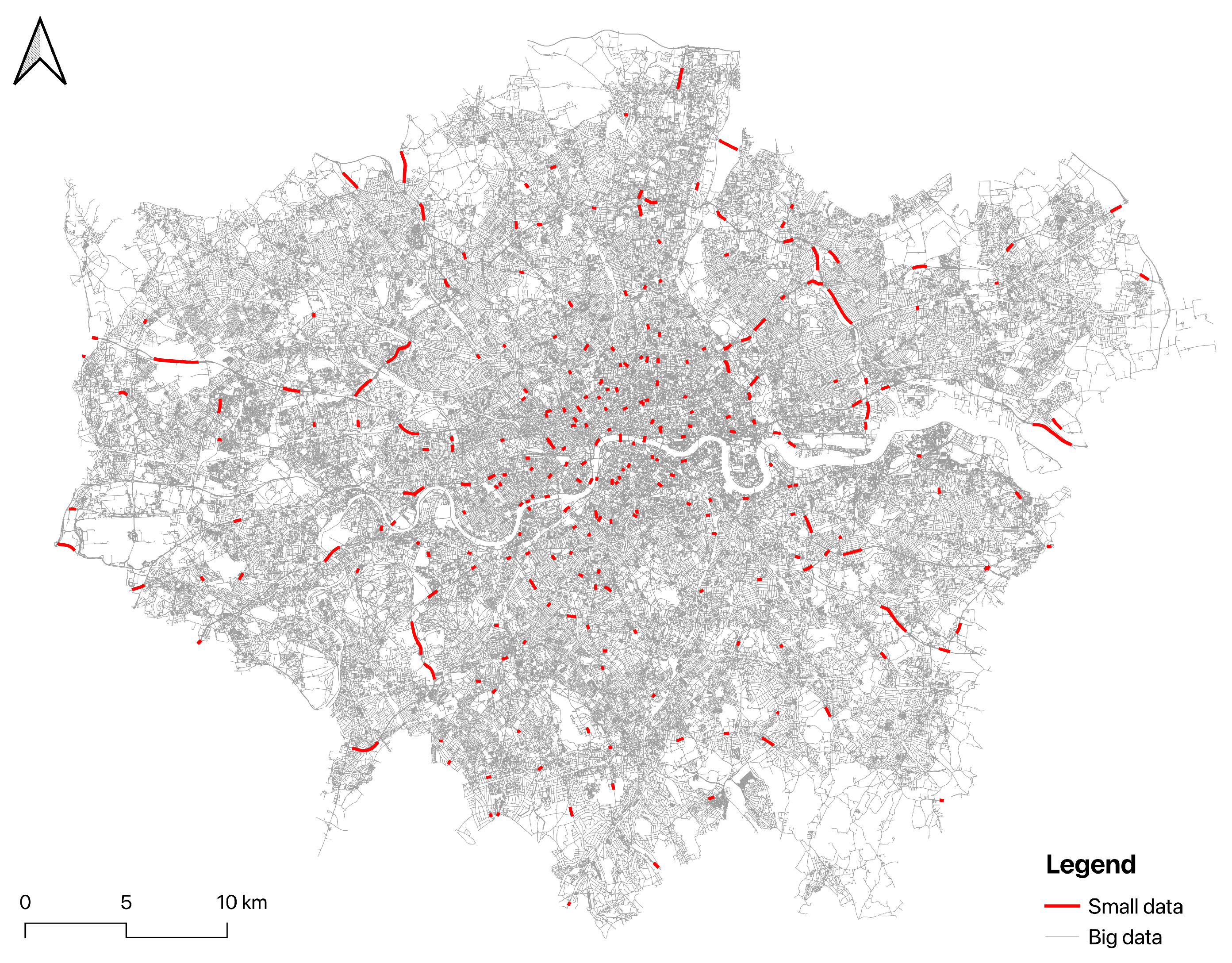
Figure 5 visualise the relationship between big data and small data, illustrating their distribution and spatial correspondence over the London road network. The two datasets used in this case study offer distinct perspectives on traffic flow, each with its advantages and limitations. Mobile phone data, derived from numerous applications, provides a broad, albeit sampled, view of traffic patterns across the entire road network, capturing a variety of travel modes and behaviours over time. This extensive coverage, however, relies on sampling methods that may not capture every nuance of traffic flow. On the other hand, the hourly traffic data from TfL, gathered through ATCs, offers precise and reliable counts of motorised traffic but is confined to fixed locations. While this method delivers high accuracy and detailed data at these points, it lacks the mobile phone data’s comprehensive network coverage, potentially missing broader traffic trends outside the areas monitored by ATCs.

5.1.2. Data Preparation

In this section, we begin by selecting roads that contain both big data and small data. For these selected roads, we divide the dataset into training, validation, and test sets in the ratio of 7:1:2 to ensure a balanced evaluation across different stages of model development.

To address the issue of small data sparsity, we implement a sliding window approach to maximise the use of available training data. Specifically, we use data from every consecutive 90-day period to fuse the traffic flow for the following day. This approach ensures that the historical information for each road is fully leveraged, allowing the model to learn from a comprehensive set of temporal patterns. Crucially, to prevent information leakage, data from the same road is confined to sets: training, validation, or test. This ensures that information from different time periods for the same road does not split across different sets, thereby maintaining the integrity of our model’s training, validation, and testing processes.

To address the issue of big data mismatch, we apply log normalisation to the initial big data to mitigate the long-tail distribution problem. The log normalisation formula used is

$$y=log(1+x)$$

(25)

where y represents the log-normalised flow value, and x represents the original flow value. This normalisation technique reduces the skewness in the data, bringing the distribution closer to a normal distribution. This step is critical for improving the performance of the model by ensuring that the data fed into it is more balanced and less prone to the distortions that can arise from highly skewed distributions. Through these data preparation steps, we aim to create a robust dataset that allows our model to effectively learn from both big and small data, ultimately improving the accuracy and reliability of the traffic flow predictions.

5.1.3. Implementation Details

The hyperparameter settings for our algorithm are provided in

Table 1. Hyperparameter settings.

Hyperparameter	Value
Batch Size	1024
Learning Rate	0.01
Epochs	50
Optimiser	Adam
Embedding Dimension for the Transformer Module	16
Embedding Dimension for Spatio-temporal Attention Layer	128
Attention Heads	2
Loss Function	MSE
Activation Function	ReLU
Batch Normalisation	True
Dropout Rate	0.1
Layer Normalisation	True
Residual Connections	True
Temporal Attention Horizon	120
Weight for the L2 Regularisation Loss	0.01

. These settings ensure that our experiments are conducted under consistent conditions. To ensure fairness in our comparisons, the hyperparameter settings for the baseline models are kept the same as those used in our algorithm, and we record the most effective results. This approach ensures consistency and reproducibility. For hyperparameters unique to our proposed model, such as the number of attention heads and hidden dimensions, we conducted grid search on the validation set to select optimal values. We also employed early stopping with a patience of five epochs, stopping training when validation loss did not improve for five consecutive epochs, to avoid overfitting. Our experiments are conducted on a Linux platform with an AMD Ryzen 9 5950X 16-Core Processor and an NVIDIA TITAN RTX GPU with 24 GB of GPU memory. We use Python 3.7.3 and PyTorch 1.13.1 for implementing our models.

5.1.4. Baselines

While the primary focus of our research is on a novel data fusion task, the underlying architectures of several well-established prediction models offer significant insights and utility for our purposes. Even though these models are traditionally used for prediction, their network structures can be effectively adapted for data fusion tasks, providing robust frameworks for integrating diverse data streams. Notably, these methods do not employ a LAN to construct an STFM, but instead use the raw data directly as input. Below is a brief introduction of the benchmark models:

• RNN: A recurrent neural network model designed to capture temporal dependencies in flow data.
• Transformer [34]: A transformer-based model that utilises self-attention mechanisms to model temporal dependencies in data.
• ST-Transformer [35]: A novel spatio-temporal transformer architecture that generates predictions autoregressively using decoupled temporal and spatial self-attention mechanisms.
• STTNs [36]: Spatial–temporal transformer networks (STTNs) that improve long-term flow forecasting accuracy by dynamically modelling time-varying spatial dependencies and long-range temporal dependencies.

By evaluating our method against these benchmark models, we aim to provide a comprehensive assessment of its effectiveness and highlight the advancements achieved through our proposed framework.

5.1.5. Evaluation Metrics

When evaluating the performance of predictive models, common performance metrics include Mean Absolute Error (MAE), Mean Absolute Percentage Error (MAPE), Root Mean Squared Error (RMSE), and Accuracy.

Mean Absolute Error (MAE). The Mean Absolute Error is the average of the absolute differences between the predicted values and the actual values. It reflects the average magnitude of errors in a set of predictions. The formula for MAE is as follows:

$$\mathrm{MAE}={\displaystyle \frac{1}{n}}\sum _{i=1}^n\left|y_i-{\widehat{y}}_i\right|$$

(26)

where n is the number of samples, $y_i$ is the actual value of the i-th sample, and ${\widehat{y}}_i$ is the predicted value of the i-th sample.

Mean Absolute Percentage Error (MAPE). The Mean Absolute Percentage Error is the average of the absolute percentage errors between the predicted values and the actual values. It is often used to assess the accuracy of a forecasting method. The formula for MAPE is as follows:

$$\mathrm{MAPE}={\displaystyle \frac{1}{n}}\sum _{i=1}^n\left|{\displaystyle \frac{y_i-{\widehat{y}}_i}{y_i}}\right|\times 100\%$$

(27)

It is important to note that MAPE can produce extremely large errors when actual values $y_i$ are close to zero.

Root Mean Squared Error (RMSE). The Root Mean Square Error is the square root of the average of the squared differences between the predicted values and the actual values. RMSE gives a higher weight to larger errors, emphasising significant deviations. The formula for RMSE is as follows:

$$\mathrm{RMSE}=\sqrt{{\displaystyle \frac{1}{n}}\sum _{i=1}^n{(y_i-{\widehat{y}}_i)}^2}$$

(28)

where n is the number of samples, $y_i$ is the actual value of the i-th sample, and ${\widehat{y}}_i$ is the predicted value of the i-th sample.

Accuracy (ACC). The Accuracy metric measures the proportion of predictions that are within 10% of the true values [4]. It is calculated as follows:

$$Accuracy={\displaystyle \frac{{\sum }_{i=1}^n⊮\left(\left|\frac{y_i-\widehat{y_i}}{y_i}\right|\le 0.1\right)}{n}}$$

(29)

where $⊮$ is the indicator function that returns 1 if the condition is true and 0 otherwise.

5.2. Experimental Results

We conducted comparative experiments with the aforementioned baselines on a real-world dataset under a zero-shot setting. This means that the roads encountered during testing were not seen during training. To ensure fairness, all experiments were conducted using the same five seeds (42–46), and we recorded the average performance on the test set when the validation set loss was at its minimum.

Table 2. Performance comparison with baseline algorithms on the real-world dataset.

Dataset	Model	Evaluation Metrics
		MAE↓	MAPE↓	RMSE↓	ACC↑
London Car Flow Dataset	RNN	0.579 ± 0.068	0.052 ± 0.006	0.660 ± 0.078	84.433 ± 5.184
	Transformer	0.592 ± 0.065	0.053 ± 0.005	0.676 ± 0.075	82.959 ± 6.058
	ST-Transformer	0.672 ± 0.131	0.060 ± 0.011	0.781 ± 0.130	76.723 ± 8.690
	STTN	0.743 ± 0.193	0.066 ± 0.016	0.860 ± 0.241	74.009 ± 4.799
	MCST-DF (Ours)	0.476 ± 0.029	0.042 ± 0.002	0.545 ± 0.032	89.879 ± 2.941

shows a performance comparison between our method and the baseline models, where bold indicates the best results.

From the results in Table 2, we can draw several key observations. First, our proposed RSTTNet method significantly outperforms all baseline models across all evaluation metrics, including Mean Absolute Error (MAE), Mean Absolute Percentage Error (MAPE), and Root Mean Square Error (RMSE). Specifically, RSTTNet achieves the lowest MAE of 0.483, the lowest MAPE of 0.043, and the lowest RMSE of 0.551, providing more accurate predicted flows compared to baseline models. It is important to note that the results shown in Table 2 are based on the test dataset corresponding to the lowest validation loss, rather than selecting the best-performing test data directly. This approach ensures that the evaluation reflects a more generalisable performance rather than overfitting to the test dataset.

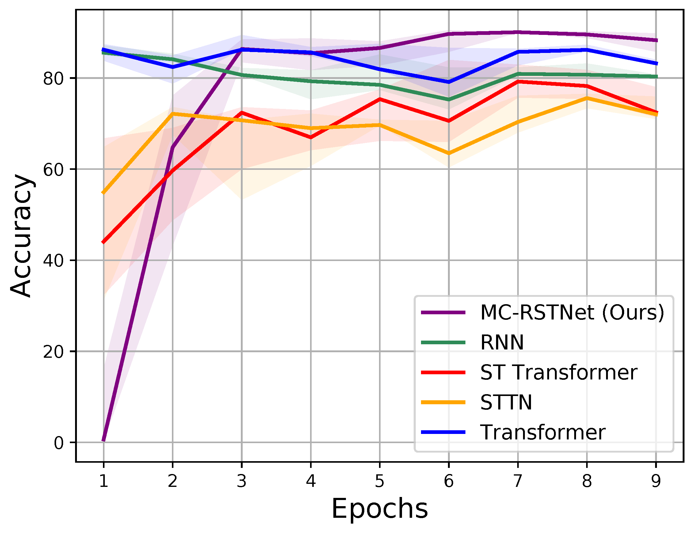
In addition, Figure 6 provides a visual comparison of the mean accuracy for each method, represented by solid lines, with the interquartile range (25–75% percentile) shaded. This figure further illustrates the robustness and reliability of RSTTNet, as it consistently demonstrates higher win rates compared to other models.

In comparison, while the RNN model is the second-best performer, it still lags behind RSTTNet by a notable margin, particularly in terms of MAE and RMSE. The transformer-based models, though generally effective, do not achieve the same level of performance, further emphasising the advantages of our approach. This discrepancy may be due to their failure to fully exploit the spatio-temporal relationships between big data and small data, as well as their lack of adequate handling of key challenges in data fusion tasks such as the mismatch of big data and the sparsity of small data.

Although the RNN model outperforms the transformer in Table 2, the MCST-DF framework is built around the transformer due to its ability to capture long-range dependencies, efficiently integrate heterogeneous data, and leverage parallel processing for large-scale networks. While RNNs perform well in standalone time series forecasting, they struggle with long-distance interactions and are less efficient for network-wide spatio-temporal data fusion. The transformer-based RSTTNet in MCST-DF effectively models complex relationships between “big” and “small” data, leading to superior overall performance in network flow estimation.

These results highlight the efficacy of our proposed method in capturing complex spatio-temporal dynamics and effectively integrating big data and small data. The marked improvement over traditional models and even advanced Transformer-based models suggests that the innovations in our RSTTNet architecture, including the use of small data modelling and residual connection, play a crucial role in enhancing predictive performance. In conclusion, the experimental analysis clearly demonstrates the superiority of RSTTNet in network flow data fusion tasks, validating its effectiveness and robustness in real-world applications.

5.3. Validation

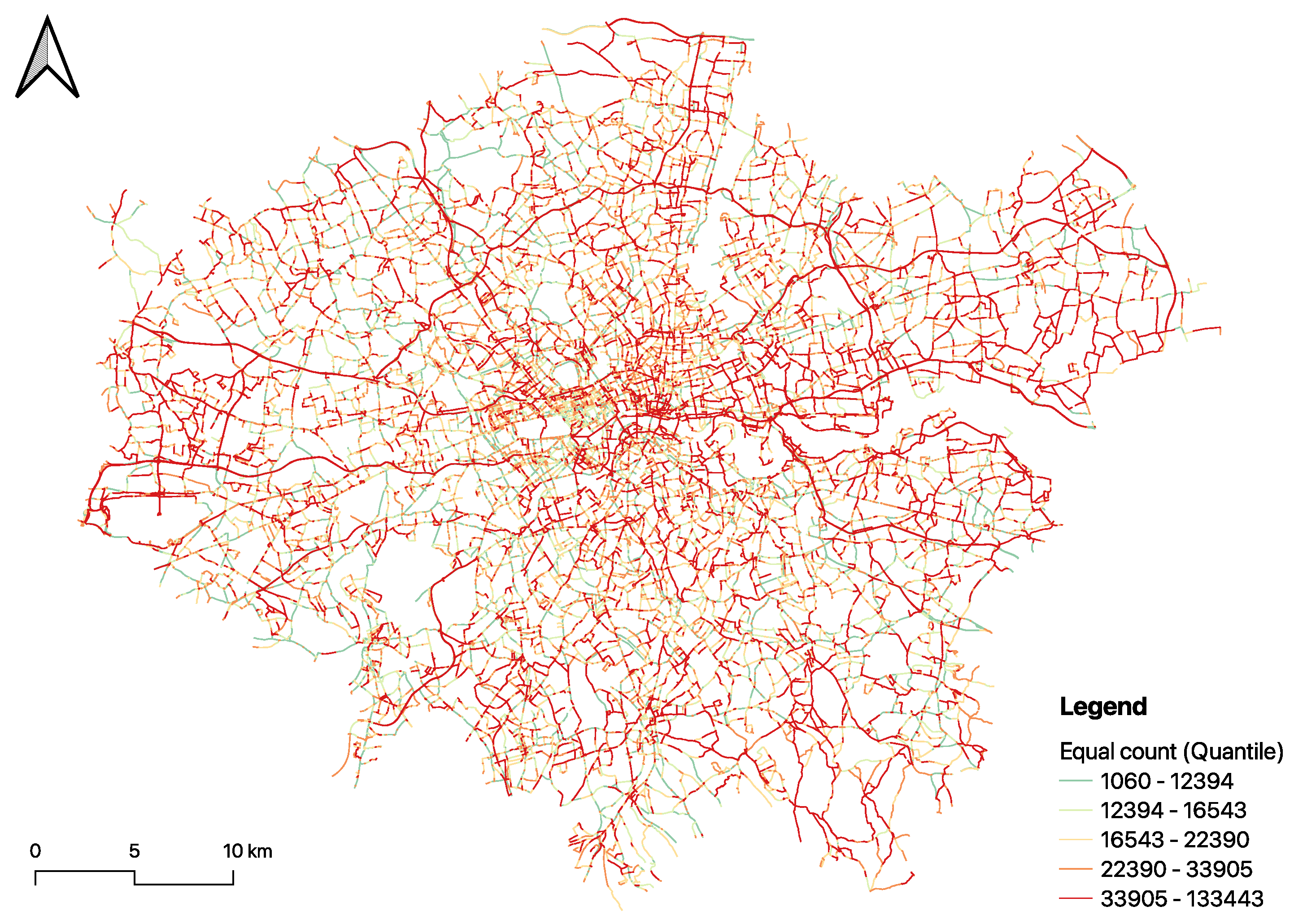
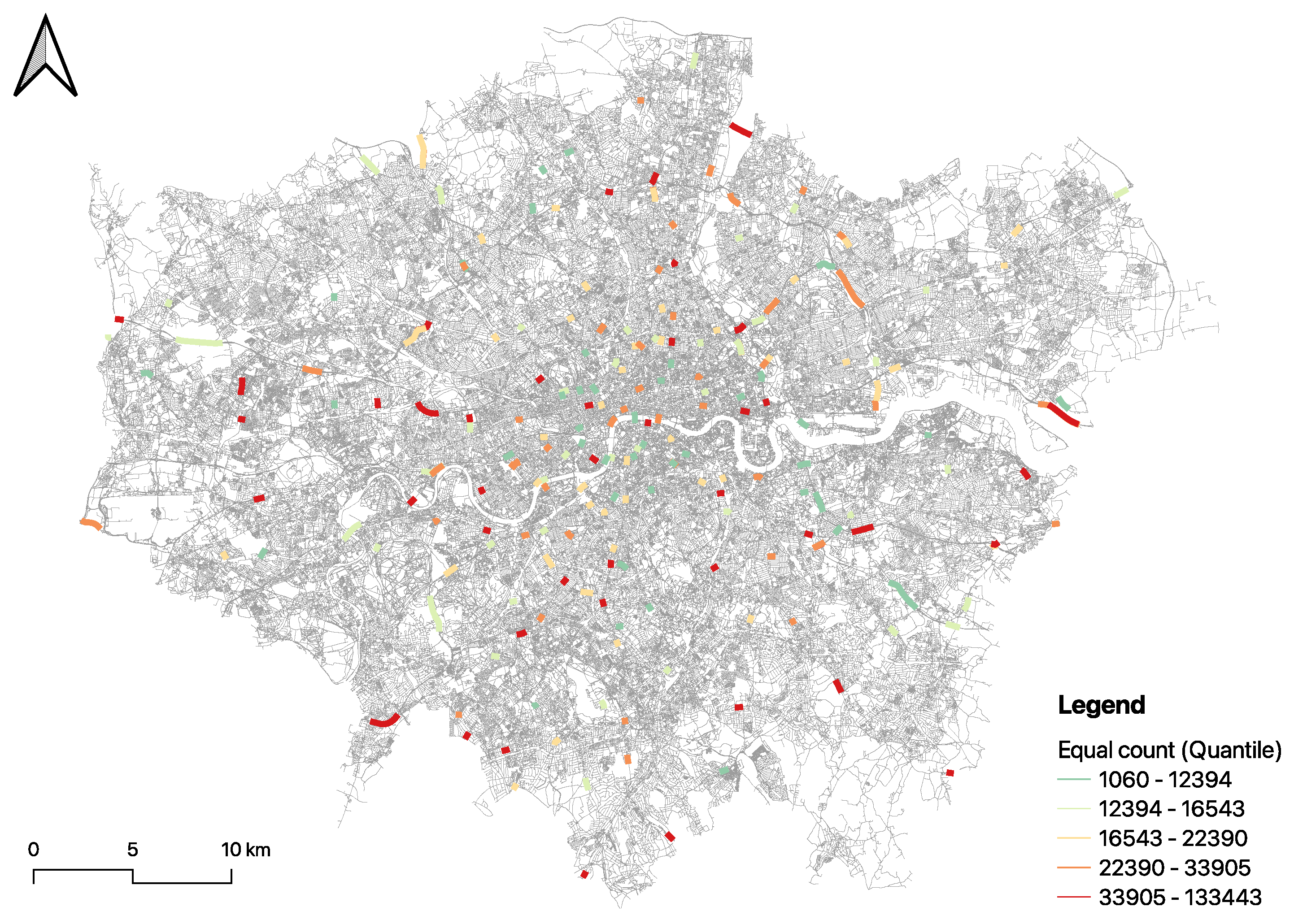
We predicted the real car flow on the TfL’s Common Operation Road Network (CORN) using the aforementioned dataset and visualised the results. Figure 7 presents a visualisation of car flow trends in London on 17 June 2024. The spatial distribution of traffic generally aligns with well-understood traffic patterns and the existing infrastructure layout in London. The traffic flow is notably dense along major transport corridors and strategic roads, such as the North Circular (A406), while local roads exhibit significantly lower traffic volumes. Additionally, our results are consistent with the visualisation of the real small data flow, as shown in Figure 8, thereby indicating the accuracy of our predictions.

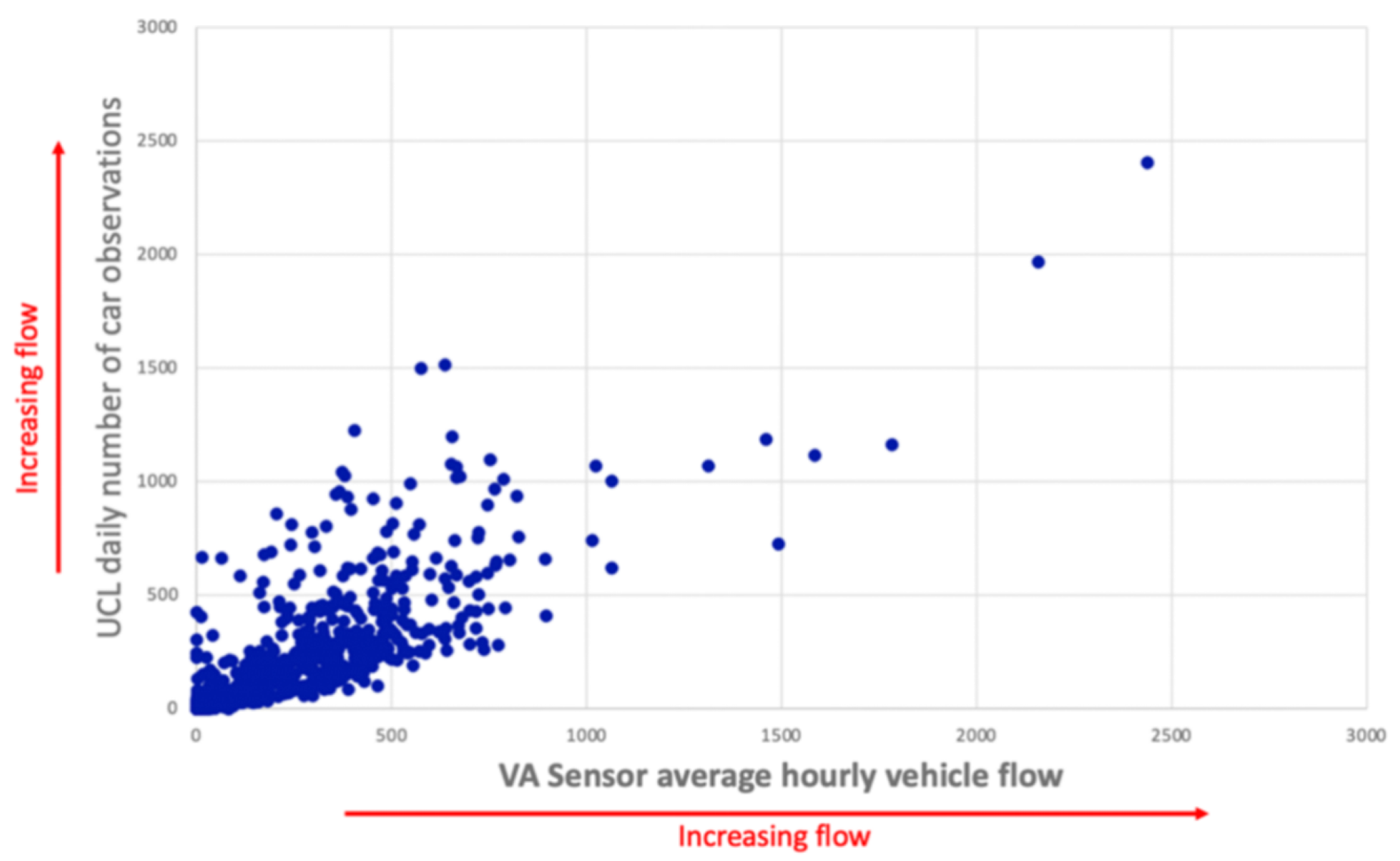
Driving flow data derived from a mobile phone application has been validated by Transport for London (TfL). TfL utilises hourly vehicle flow data from 615 road links, incorporating sensors from TfL and 10 London boroughs. The collected data spans all road hierarchies, including A Road Primary (40), A Road (231), B Road (62), Minor Road (92), and Local Road (190). According to TfL’s validation, the driving flow derived from the mobile phone application exhibits a strong correlation with officially collected flow data, with an overall correlation of 0.78 (without outlier removal). However, due to TfL’s restrictions, these validation results will not be included in the article.

While the validation confirms a high degree of accuracy, it is important to acknowledge the limitations and potential biases inherent in the mobile phone dataset. For instance, data coverage may be skewed due to uneven smartphone penetration across age groups, socioeconomic status, or geographic regions. Individuals who do not use location-enabled applications or who use less common devices (e.g., non-Android or privacy-focused phones) may be underrepresented. These factors should be considered when interpreting the results, and future work may benefit from complementary datasets or correction techniques to address these disparities. The correlation between UCL mobile application-derived vehicle flow and TfL sensor data is illustrated in Figure 9.

5.4. Analysis

5.4.1. Sensitivity Analysis

We further examine whether our proposed algorithm is sensitive to different parameter settings. We conduct experiments to test how the model performance varies with different numbers of attention layers, hidden dimensions and attention heads. In the following, we present a detailed analysis of the results obtained for various configurations, followed by a summary and conclusion on the sensitivity of our model.

As shown in

Table 3. Performance comparison with varying numbers of attention layers on the real-world dataset.

Dataset	Model	Evaluation Metrics
		MAE↓	MAPE↓	RMSE↓	ACC↑
London Car Flow Dataset	Attention Layers = 1	0.476 ± 0.029	0.042 ± 0.002	0.545 ± 0.032	89.879 ± 2.941
	Attention Layers = 2	0.494 ± 0.020	0.044 ± 0.001	0.566 ± 0.021	89.146 ± 2.986
	Attention Layers = 3	0.516 ± 0.076	0.046 ± 0.006	0.585 ± 0.081	87.805 ± 4.769

, we first analyze the impact of varying the number of attention layers. The results indicate that the model achieves the best performance with one attention layer, resulting in the lowest MAE of 0.483, MAPE of 0.043, and RMSE of 0.551. As the number of attention layers increases to 2 and 3, the performance slightly deteriorates, with MAE increasing to 0.494 and 0.516, respectively. This suggests that while a single attention layer is sufficient for capturing the necessary spatio-temporal dynamics, adding more layers may introduce unnecessary complexity, leading to overfitting.

Next, in

Table 4. Performance comparison with varying hidden dimension sizes on the real-world dataset.

Dataset	Model	Evaluation Metrics
		MAE↓	MAPE↓	RMSE↓	ACC↑
London Car Flow Dataset	Hidden Dim = 2	0.497 ± 0.080	0.045 ± 0.006	0.566 ± 0.080	89.151 ± 6.237
	Hidden Dim = 4	0.558 ± 0.196	0.050 ± 0.017	0.627 ± 0.195	85.954 ± 9.108
	Hidden Dim = 16	0.476 ± 0.029	0.042 ± 0.002	0.545 ± 0.032	89.879 ± 2.941

, we examine the effect of varying the hidden dimension size on model performance. The results show that the hidden dimension of 16 yields the best results with the lowest MAE of 0.483, MAPE of 0.043, and RMSE of 0.551. When the hidden dimension is reduced to 2 or increased to 4, the model’s performance declines, indicating that a hidden dimension of 16 strikes the optimal balance between model complexity and capacity.

Lastly,

Table 5. Performance comparison with varying numbers of attention heads on the real-world dataset.

Dataset	Model	Evaluation Metrics
		MAE↓	MAPE↓	RMSE↓	ACC↑
London Car Flow Dataset	Attention Heads = 1	0.479 ± 0.047	0.043 ± 0.004	0.549 ± 0.048	90.198 ± 4.657
	Attention Heads = 2	0.483 ± 0.055	0.043 ± 0.005	0.551 ± 0.059	89.965 ± 3.321
	Attention Heads = 4	0.476 ± 0.029	0.042 ± 0.002	0.545 ± 0.032	89.879 ± 2.941

presents the performance comparison when varying the number of attention heads. The results show that while the model achieves slightly better performance with four attention heads, resulting in the lowest MAE of 0.469, MAPE of 0.042, and RMSE of 0.541, the differences between configurations with one and two attention heads are minimal. This suggests that the network’s performance is relatively insensitive to the number of attention heads, indicating that this parameter does not significantly impact the model’s ability to capture the intricate relationships within the data.

In summary, the sensitivity analysis reveals that our proposed RSTTNet model is robust across various configurations, yet certain parameters significantly impact its performance. Specifically, the best results are obtained with one attention layer, a hidden dimension size of 16, and four attention heads. These findings highlight the importance of careful tuning of the model’s architecture to fully leverage its strengths in capturing complex spatio-temporal dependencies. Overall, our RSTTNet method demonstrates superior performance and robustness, confirming its effectiveness in network flow data fusion tasks.

5.4.2. Ablation Studies

We conduct ablation studies to assess the necessity and impact of each component in our proposed RSTTNet model.

Table 6. Performance comparison with ablation algorithms on the real-world dataset.

Dataset	Model	Evaluation Metrics
		MAE↓	MAPE↓	RMSE↓	ACC↑
London Car Flow Dataset	No Layered Attention Network	0.564 ± 0.169	0.051 ± 0.010	0.651 ± 0.168	84.816 ± 8.501
	No Small Data Modelling	0.566 ± 0.073	0.050 ± 0.006	0.640 ± 0.079	84.612 ± 4.480
	Linear Small Data Modelling	0.517 ± 0.131	0.046 ± 0.012	0.589 ± 0.176	87.085 ± 9.998
	MCST-DF (Ours)	0.476 ± 0.029	0.042 ± 0.002	0.545 ± 0.032	89.879 ± 2.941

presents a performance comparison across different variations of our model on the real-world dataset. Figure 10 provides a visual comparison of the mean accuracy for each method, represented by solid lines, with the interquartile range (25–75% percentile) shaded. Below, we describe each variation and its corresponding results in detail.

• No Layered Attention Network: In this variation, the Layered Attention Network is removed, but zero padding is retained for easier processing. This configuration results in an MAE of 0.564, a MAPE of 0.051, and an RMSE of 0.651. The higher error metrics indicate that the absence of the Layered Attention Network hampers the model’s ability to capture complex spatio-temporal relationships.
• No small data modelling: This variant removes the specialised small data modelling component. It yields an MAE of 0.566, a MAPE of 0.050, and an RMSE of 0.640. The slightly worse performance compared to other variants suggests that small data modelling is essential for effectively integrating sparse and accurate small data with large-scale but noisy big data.
• Linear small data modelling: In this version, the transformer network in the small data modelling module is replaced with a simpler linear model. This configuration achieves an MAE of 0.517, a MAPE of 0.046, and an RMSE of 0.589. While this approach performs better than the previous two variants, it still does not match the full RSTTNet model, underscoring the importance of using more advanced small data modelling techniques.
• RSTTNet: The complete RSTTNet model, which includes both the Layered Attention Network and advanced small data modelling, achieves the best performance across all metrics, with an MAE of 0.483, a MAPE of 0.043, and an RMSE of 0.551. These results highlight the effectiveness of the full model configuration in capturing spatio-temporal dependencies and integrating heterogeneous data sources.

In summary, the ablation studies clearly demonstrate that both the Layered Attention Network and the advanced small data modelling components are essential to achieving superior predictive performance. The full RSTTNet model significantly outperforms its ablated variants, validating the design choices made in developing our method. Also, the proposed Multi-Channel Spatio-Temporal Data Fusion (MCST-DF) framework along with its components, multi-chanel spatio-temporal feature mapping, effectively addresses the issues of mismatch, sparsity, and heterogeneity.

The MCST-DF framework specifically addresses the issue of mismatch by extracting the spatio-temporal features from the big data then combined with the small data through the RSTTNet. This underscores the framework’s capability in enhancing overall data accuracy. Regarding sparsity, the transformer-based small data modelling approach effectively utilises sparse and geographically limited data, which is evident from the improvement in model performance when compared to configurations without small data modelling. Lastly, the heterogeneity challenge is tackled through the Layered Attention Network which embeds multi-channel spatio-temporal features, allowing for a better understanding of complex data structures. This is demonstrated by the advanced modelling capabilities of RSTTNet, which outperforms the variant without the Layered Attention Network in all key metrics, supporting its effectiveness in handling diverse data types and structures.

6. Conclusions and Future Work

This study addresses a fundamental challenge in spatio-temporal data integration: how to effectively fuse large-scale, passively collected “big” data with sparse, high-quality “small” data to reconstruct underlying network dynamics. We proposed the Multi-Channel Spatio-Temporal Data Fusion (MCST-DF) framework, underpinned by a novel Residual Spatio-Temporal Transformer Network (RSTTNet). The framework leverages the complementary strengths of both data types to capture complex spatial and temporal dependencies while mitigating issues of sampling bias and data sparsity.

Empirical evaluation on a real-world urban road network demonstrates significant improvements in predictive accuracy compared to baseline deep learning models, confirming the effectiveness of our approach for intelligent mobility monitoring and geospatial data enrichment. By addressing a pressing need in GeoAI—the fusion of heterogeneous spatio-temporal data—this work contributes to advancing scalable solutions for smart cities, infrastructure resilience, and network state estimation.

Future work will focus on extending this framework to incorporate multimodal data sources, including real-time imagery, environmental sensors, and social media feeds. Such integration will enable richer representations of urban dynamics and support advanced tasks such as anomaly detection, flow forecasting, and policy-driven simulation. Ultimately, our goal is to develop robust, transferable data fusion techniques that support decision-making in increasingly complex and data-rich geospatial systems. Furthermore, although this study focuses on traffic flow estimation, we believe the proposed framework can be generalised to other spatio-temporal data fusion tasks, and we plan to explore its application to domains such as environmental monitoring and urban sensing in future research. In addition, evaluating the generalisability of the proposed framework in diverse settings will be an important direction for future work, enabling further demonstration of its robustness and broad applicability.

References

- Li, S.; Dragicevic, S.; Castro, F.A.; Sester, M.; Winter, S.; Coltekin, A.; Pettit, C.; Jiang, B.; Haworth, J.; Stein, A.; et al. Geospatial big data handling theory and methods: A review and research challenges. ISPRS J. Photogramm. Remote Sens. 2016, 115, 119–133. [Google Scholar] [CrossRef]
- Zheng, Y. Methodologies for cross-domain data fusion: An overview. IEEE Trans. Big Data 2015, 1, 16–34. [Google Scholar] [CrossRef]
- Liu, J.; Li, T.; Xie, P.; Du, S.; Teng, F.; Yang, X. Urban big data fusion based on deep learning: An overview. Inf. Fusion 2020, 53, 123–133. [Google Scholar] [CrossRef]
- Kashinath, S.A.; Mostafa, S.A.; Mustapha, A.; Mahdin, H.; Lim, D.; Mahmoud, M.A.; Mohammed, M.A.; Al-Rimy, B.A.S.; Fudzee, M.F.M.; Yang, T.J. Review of data fusion methods for real-time and multi-sensor traffic flow analysis. IEEE Access 2021, 9, 51258–51276. [Google Scholar] [CrossRef]
- Zhang, Y.D.; Dong, Z.; Wang, S.H.; Yu, X.; Yao, X.; Zhou, Q.; Hu, H.; Li, M.; Jiménez-Mesa, C.; Ramirez, J.; et al. Advances in multimodal data fusion in neuroimaging: Overview, challenges, and novel orientation. Inf. Fusion 2020, 64, 149–187. [Google Scholar] [CrossRef]
- Di Curzio, D.; Castrignanò, A.; Fountas, S.; Romić, M.; Rossel, R.A.V. Multi-source data fusion of big spatial-temporal data in soil, geo-engineering and environmental studies. Sci. Total Environ. 2021, 788, 147842. [Google Scholar] [CrossRef]
- Maragos, P.; Gros, P.; Katsamanis, A.; Papandreou, G. Cross-modal integration for performance improving in multimedia: A review. In Multimodal Processing and Interaction: Audio, Video, Text; Springer: Boston, MA, USA, 2008; pp. 1–46. [Google Scholar]
- Liang, Y.; Zhao, Z.; Sun, L. Memory-augmented dynamic graph convolution networks for traffic data imputation with diverse missing patterns. Transp. Res. Part C Emerg. Technol. 2022, 143, 103826. [Google Scholar] [CrossRef]
- Wang, A.; Ye, Y.; Song, X.; Zhang, S.; James, J. Traffic prediction with missing data: A multi-task learning approach. IEEE Trans. Intell. Transp. Syst. 2023, 24, 4189–4202. [Google Scholar] [CrossRef]
- Cui, Z.; Lin, L.; Pu, Z.; Wang, Y. Graph Markov network for traffic forecasting with missing data. Transp. Res. Part C Emerg. Technol. 2020, 117, 102671. [Google Scholar] [CrossRef]
- Guo, S.; Lin, Y.; Wan, H.; Li, X.; Cong, G. Learning dynamics and heterogeneity of spatial-temporal graph data for traffic forecasting. IEEE Trans. Knowl. Data Eng. 2021, 34, 5415–5428. [Google Scholar] [CrossRef]
- Zhang, L.; Xie, Y.; Xidao, L.; Zhang, X. Multi-source heterogeneous data fusion. In Proceedings of the 2018 International Conference on Artificial Intelligence and Big Data (ICAIBD), Chengdu, China, 26–28 May 2018; pp. 47–51. [Google Scholar]
- Zhang, J.; Zheng, Y.; Qi, D. Deep spatio-temporal residual networks for citywide crowd flows prediction. In Proceedings of the AAAI Conference on Artificial Intelligence, San Francisco, CA, USA, 4–9 February 2017; Volume 31. [Google Scholar]
- Yi, X.; Zhang, J.; Wang, Z.; Li, T.; Zheng, Y. Deep distributed fusion network for air quality prediction. In Proceedings of the 24th ACM SIGKDD International Conference on Knowledge Discovery & Data Mining, London, UK, 19–23 August 2018; pp. 965–973. [Google Scholar]
- Du, S.; Li, T.; Gong, X.; Horng, S.J. A hybrid method for traffic flow forecasting using multimodal deep learning. Int. J. Comput. Intell. Syst. 2020, 13, 85–97. [Google Scholar] [CrossRef]
- Feng, S.; Wei, S.; Zhang, J.; Li, Y.; Ke, J.; Chen, G.; Zheng, Y.; Yang, H. A macro–micro spatio-temporal neural network for traffic prediction. Transp. Res. Part C Emerg. Technol. 2023, 156, 104331. [Google Scholar] [CrossRef]
- Li, M.; Zhu, Z. Spatial-temporal fusion graph neural networks for traffic flow forecasting. In Proceedings of the AAAI Conference on Artificial Intelligence, Virtual, 2–9 February 2021; Volume 35, pp. 4189–4196. [Google Scholar]
- Liu, J.; Ong, G.P.; Chen, X. GraphSAGE-based traffic speed forecasting for segment network with sparse data. IEEE Trans. Intell. Transp. Syst. 2020, 23, 1755–1766. [Google Scholar] [CrossRef]
- Lu, L.; Wang, J.; He, Z.; Chan, C.Y. Real-time estimation of freeway travel time with recurrent congestion based on sparse detector data. IET Intell. Transp. Syst. 2018, 12, 2–11. [Google Scholar] [CrossRef]
- Wang, S.; Zhang, X.; Cao, J.; He, L.; Stenneth, L.; Yu, P.S.; Li, Z.; Huang, Z. Computing urban traffic congestions by incorporating sparse GPS probe data and social media data. ACM Trans. Inf. Syst. 2017, 35, 1–30. [Google Scholar] [CrossRef]
- Benkraouda, O.; Thodi, B.T.; Yeo, H.; Menendez, M.; Jabari, S.E. Traffic data imputation using deep convolutional neural networks. IEEE Access 2020, 8, 104740–104752. [Google Scholar] [CrossRef]
- Yu, B.; Yin, H.; Zhu, Z. Spatio-temporal graph convolutional networks: A deep learning framework for traffic forecasting. arXiv 2017, arXiv:1709.04875. [Google Scholar]
- Li, Y.; Yu, R.; Shahabi, C.; Liu, Y. Diffusion convolutional recurrent neural network: Data-driven traffic forecasting. arXiv 2017, arXiv:1707.01926. [Google Scholar]
- Guo, S.; Lin, Y.; Feng, N.; Song, C.; Wan, H. Attention based spatial-temporal graph convolutional networks for traffic flow forecasting. In Proceedings of the AAAI Conference on Artificial Intelligence, Honolulu, HI, USA, 27 January–1 February 2019; Volume 33, pp. 922–929. [Google Scholar]
- Lv, M.; Hong, Z.; Chen, L.; Chen, T.; Zhu, T.; Ji, S. Temporal multi-graph convolutional network for traffic flow prediction. IEEE Trans. Intell. Transp. Syst. 2020, 22, 3337–3348. [Google Scholar] [CrossRef]
- Anselin, L. Local indicators of spatial association—LISA. Geogr. Anal. 1995, 27, 93–115. [Google Scholar] [CrossRef]
- Zhang, Y.; Cheng, T.; Ren, Y. A graph deep learning method for short-term traffic forecasting on large road networks. Comput.-Aided Civ. Infrastruct. Eng. 2019, 34, 877–896. [Google Scholar] [CrossRef]
- Gao, X.; Jiang, X.; Haworth, J.; Zhuang, D.; Wang, S.; Chen, H.; Law, S. Uncertainty-aware probabilistic graph neural networks for road-level traffic crash prediction. Accid. Anal. Prev. 2024, 208, 107801. [Google Scholar] [CrossRef]
- Nejad, A.S.; Alaiz-Rodríguez, R.; McCarthy, G.D.; Kelleher, B.; Grey, A.; Parnell, A. SERT: A Transfomer Based Model for Spatio-Temporal Sensor Data with Missing Values for Environmental Monitoring. arXiv 2023, arXiv:2306.03042. [Google Scholar]
- He, K.; Zhang, X.; Ren, S.; Sun, J. Deep residual learning for image recognition. In Proceedings of the IEEE Conference on Computer Vision and Pattern Recognition, Las Vegas, NV, USA, 27–30 June 2016; pp. 770–778. [Google Scholar]
- Zhang, X.; Cheng, T. Unlocking the Power of Mobile Phone Application Data to Accelerate Transport Decarbonisation (Short Paper). In Proceedings of the 12th International Conference on Geographic Information Science (GIScience 2023), Leeds, UK, 12–15 September 2023. [Google Scholar]
- Bolbol, A.; Cheng, T.; Tsapakis, I.; Haworth, J. Inferring hybrid transportation modes from sparse GPS data using a moving window SVM classification. Comput. Environ. Urban Syst. 2012, 36, 526–537. [Google Scholar] [CrossRef]
- Transport for London. Freedom of Information Request Detail. 2024. Available online: https://discovery.ucl.ac.uk/id/eprint/10209012/ (accessed on 6 September 2024).
- Vaswani, A.; Shazeer, N.; Parmar, N.; Uszkoreit, J.; Jones, L.; Gomez, A.N.; Kaiser, Ł.; Polosukhin, I. Attention is all you need. Adv. Neural Inf. Process. Syst. 2017, 30, 5998. [Google Scholar]
- Aksan, E.; Kaufmann, M.; Cao, P.; Hilliges, O. A spatio-temporal transformer for 3d human motion prediction. In Proceedings of the 2021 International Conference on 3D Vision (3DV), London, UK, 1–3 December 2021; pp. 565–574. [Google Scholar]
- Xu, M.; Dai, W.; Liu, C.; Gao, X.; Lin, W.; Qi, G.J.; Xiong, H. Spatial-temporal transformer networks for traffic flow forecasting. arXiv 2020, arXiv:2001.02908. [Google Scholar]