Accelerating Computation for Estimating Land Surface Temperature: An Efficient Global–Local Regression (EGLR) Framework

Abstract

Rapid urbanization elevates land surface temperature (LST) through complex urban spatial relationships, intensifying the urban heat island (UHI) effect. This necessitates efficient methods to analyze surface urban heat island (SUHI) factors to help develop mitigation strategies. In this study, we propose an efficient global–local regression (EGLR) framework by integrating XGBoost-SHAP with global–local regression (GLR), enabling accelerated estimation of LST. In a case study of Wuhan, the EGLR reduces the computation time of GLR by 44.21%. The main contribution of computational efficiency improvement lies in the procedure of Moran eigenvector selecting executed by XGBoost-SHAP. Results of validation experiments also show significant time decrease of the EGLR for a larger sample size; in addition, transplanting the framework of the EGLR to two machine learning models not only reduces the executing time, but also increases model fitting. Furthermore, the inherent merits of XGBoost-SHAP and GLR also enables the EGLR to simultaneously capture nonlinear causal relationships and decompose spatial effects. Results identify population density as the most sensitive LST-increasing factor. Impervious surface percentage, building height, elevation, and distance to the nearest water body are positively correlated with LST, while water area, normalized difference vegetation index, and the number of bus stops have significant negative relationships with LST. In contrast, the impact of the number of points of interest, gross domestic product, and road length on LST is not significant overall.

1. Introduction

Over the past decade, extensive urban expansion and worldwide population growth have triggered a series of environmental challenges, among which the urban heat island effect stands out as a prominent issue [1]. The urban heat island (UHI) effect, characterized by elevated temperatures in urban areas relative to surrounding rural regions [2], has long been recognized as a significant threat to the health of urban residents [3]. This phenomenon is intricately linked to summer heatwaves [4], air pollution [5,6], energy consumption [7], biodiversity loss [8], and human health and comfort [9]. With substantial evidence indicating increased health risks and mortality rates [10,11], these multifaceted impacts pose severe challenges to the sustainable development of cities. Therefore, analyzing the UHI effect is crucial for guiding the sustainable development of cities.

UHIs are mainly divided into the urban canopy layer (UCL), urban boundary layer (UBL), and surface urban heat island (SUHI) [12]. Research on UCL and UBL typically relies on complex monitoring equipment and dense observational networks, making it challenging to achieve high-precision studies. In contrast, SUHI has been extensively investigated due to the advantages of continuous satellite image coverage, accessibility, and the development of GIS software packages [13]. Numerous land surface temperature (LST) datasets are currently available, such as high-resolution Landsat 8 data products and the Moderate Resolution Imaging Spectroradiometer (MODIS) MOD11A1 or MOD11A2 products.

It is widely acknowledged that the UHI effect arises from two primary factors. On one hand, intensive human activities within urban areas release substantial amounts of anthropogenic heat. On the other hand, the replacement of natural vegetation, green spaces, and water bodies with impervious surfaces in urban landscapes plays a significant role. These impervious surfaces absorb considerable solar radiation during the day and gradually release it at night, leading to localized temperature increases. This process reduces evaporative cooling, impedes gas exchange between soil and the atmosphere, and restricts air circulation, collectively exacerbating the UHI phenomenon [14,15,16,17]. If the relationship between urban land surface temperature and human social activities, as well as the connection between land use and land cover, can be quantified [18,19,20], it would provide a scientific basis and decision-making support for urban planning and management, enabling the balance and improvement of the urban thermal environment.

Currently, researchers are developing various models to estimate urban land surface temperature, aiming to elucidate the underlying causes of the UHI effect. In these models, the dependent variable is typically defined as land surface temperature or air temperature, while the selection of independent variables encompasses multiple dimensions, primarily determined by the characteristics of the model and the feasibility of data acquisition. These models can be broadly categorized into two types. The first type comprises simulation models based on extensive actual measurement data, such as the urban canopy model (UCM) [21]; some studies have also attempted to integrate the UCM with climate models, such as the weather research and forecasting model (WRF) [22,23]. The other type comprises primarily data-driven regression models. With the rapid advancement of remote sensing technology and its extensive temporal and spatial coverage, regression models have been increasingly applied in the analysis of the UHI effect.

For instance, Guo et al. [24] employed spatial lag models (SLM) and spatial error models (SEM) to investigate how spatial variables of land use influence land surface temperature at the neighborhood scale, taking into account urban spatial morphology. Shahfahad et al. [25] utilized geographically weighted regression (GWR) models with Landsat datasets to analyze land use/land cover changes and their impact on surface UHI intensity and urban thermal comfort in the Delhi metropolitan area. Yang et al. [26] applied multiscale geographically weighted regression (MGWR) to examine how urban morphological factors, biophysical parameters, land use types, socioeconomics, and landscape pattern indices affect variations in land surface temperature in Fuzhou, China.

In recent years, many machine learning methods also have been used in UHI effect modeling. For example, Gao et al. [27] compared multivariate linear regression (MLR), geographically weighted regression (GWR), random forest (RF), and artificial neural networks (ANN) to establish the relationship between land use/cover and land surface temperature (LST), concluding that the fitting performance ranked as follows: RF > GWR > ANN > MLR. These machine learning models have yielded highly satisfactory results. Notably, two typical nonlinear models—RF and ANN—outperform the linear model MLR. This further confirms that incorporating nonlinear characteristics into urban heat island (UHI) modeling can more accurately reflect the actual interactions between driving factors and LST.

Classic (spatial) regression models and machine learning models possess their own strengths and limitations; by extracting and integrating the advantages of regression models, the resulting hybrid models often achieve more effective and efficient improvements. For instance, Zhang [28] proposed a hybrid time series forecasting approach that integrates the autoregressive integrated moving average (ARIMA) model with a neural network model to leverage the unique strengths of ARIMA and ANN in linear and nonlinear modeling, respectively. Jia et al. [29] developed a hybrid model that combines GWR with a deep neural network (DNN) to estimate land surface temperature, utilizing the DNN’s nonlinear modeling capabilities to model the residuals of GWR and subsequently integrating the linear and nonlinear components to estimate LST. Hagenauer et al. [30] introduced a geographically weighted artificial neural network (GWANN) model by integrating GWR with neural networks, demonstrating that GWANN outperforms GWR when the relationships within the data are nonlinear and exhibit high spatial variation. Du et al. [31] proposed a geographically neural network weighted regression (GNNWR) model, which combines ordinary least squares (OLS) with neural networks to precisely express the weighting kernel of the GWR model, achieving superior fitting accuracy and more robust predictions compared to OLS and GWR. These studies highlight the potential of hybrid models in addressing complex spatial non-stationarity across various geographical processes and environments.

Although the global–local regression (GLR) model [32], integrating GWR [33] with Moran eigenvector spatial filtering (MESF) technique [34], can capture global spatial autocorrelation and local spatial heterogeneity, it tends to be time consuming. Building on this, the present study seeks to reduce computation time by employing XGBoost-SHAP method, and to extend the conceptual framework of the efficient global–local regression (EGLR) model to machine learning models.

The main contribution of this study includes three aspects. First, the study formulates an accelerated variable selecting procedure by integrating XGBoost-SHAP methods to significantly improve the computation efficiency of global–local regression. Second, the research reveals impacting mechanisms of eleven driving factors within four categories on LST of Wuhan central areas. And third, the work extends the conceptual framework of EGLR (i.e., the efficiency improved global–local regression) to machine learning based models, enriching methodological toolkit for urban heat island analysis.

2. Study Area and Data

2.1. Study Area

The study area is within Wuhan (30°32′ N, 114°17′ E), a major metropolitan city in central China, and located at the confluence of the Yangtze River and the Han River, historically known as the “Thoroughfare of Nine Provinces.” As the capital of Hubei Province, Wuhan serves as a vital transportation hub and economic center in China (see Figure 1a). According to statistical data from 2023, Wuhan has an urbanization rate of 84.3% and a permanent resident population of 13.774 million. Based on the Köppen–Geiger climate classification [35], Wuhan experiences a subtropical monsoon climate characterized by hot, rainy summers and cold, humid winters, with an average annual temperature of approximately 16.5 °C and an annual precipitation of around 1200 mm.

However, with the rapid acceleration of urbanization, extreme climate events in Wuhan have become increasingly frequent, particularly during the summer months. For instance, in the summer of 2022, Wuhan experienced many consecutive days with extremely high temperatures exceeding 40 °C, setting a historical record. Additionally, the UHI effect in Wuhan is pronounced, with the average temperature in the city center being 3–5 °C higher than in suburban areas, especially during the night. This extreme climate phenomenon may be closely linked to the rapid urbanization process [36], where extensive artificial surfaces (e.g., buildings and roads) have replaced natural surfaces (e.g., vegetation and water bodies), leading to increased land surface temperatures and intensified heat island effects [37,38]. Therefore, the relatively central parts of Wuhan were selected as the research area (comprising approximately 2123.26 square kilometers) for this study (Figure 1). The Yangtze River runs through this area directly, naturally dividing the region into the north-west and south-east halves, which endows it with more intricate geomorphic features. Additionally, this region is predominantly covered by artificial surfaces, reflecting a high degree of urbanization and intensive economic activities.

To ensure spatial consistency and analytical precision, the study area was discretized into standardized 1 km × 1 km grid units, because 1 km × 1 km corresponds to the distance people can cover on foot within a 15-min walk [39]. Therefore, the basic research unit is the 1 km × 1 km grid, and we have 2424 such units in central areas of Wuhan.

2.2. Multi-Sourced Datasets and Variables

2.2.1. Sources of Datasets

The land surface temperature (LST) data was obtained from the MOD11A2 product, provided by the National Aeronautics and Space Administration (NASA), with a spatial resolution of 1 km and a temporal resolution of 8 days. To ensure more reliable results, multiple remote sensing images during the summer seasons (June to August) were selected for LST retrieval, as the SUHI effect is most pronounced during this period. To ensure high-quality analysis, this study utilized four cloud-free images acquired from 20 August 2020 to 27 August 2020. These images were mosaicked to achieve complete coverage of the entire study area for the investigation.

Previous studies have shown that urban form factors [26,29], land use type [26], socioeconomics [26,40], landscape metrics [29], anthropogenic activities [41], location and local climate [42], and natural environment [29,42] have significant impacts on LST. Based on prior research, we selected variables including water area (Water), normalized difference vegetation index (NDVI), gross domestic product (GDP), population density (PD), impervious surface area (ISP), the number of points of interest (POI), the number of bus stops (Station), road length (RL), building height (BH), elevation (DEM), and distance to the nearest water body (NWB).

The variables were categorized into the following groups.

(1)

Indicators of land use type

Water and NDVI variables are within this type. The Water data was obtained from the GLC_FCS30D product [43], which provides detailed classification of 35 land cover types at 30-m spatial resolution (resampled to 1 km). The NDVI data was derived from the MOD13A3 dataset, where the annual average NDVI for 2020 was calculated by averaging monthly Normalized Difference Vegetation Index values across 12 months.

(2)

Socioeconomic indicators

GDP and PD were employed as socioeconomic indicators. We collected GDP data from Zhao et al. [44] which provides China’s GDP at the pixel level using nighttime lights time series and population images. The PD data with 1 km resolution was obtained from the LandScan platform.

(3)

Urban Form Factors

ISP, POI, Stations, RL, and BH were collected as urban form factors. These were extracted from: the GLC_FCS30D product, Baidu Maps API, OpenStreetMap, and the Zenodo database [45], respectively.

(4)

Natural environmental factors

We collected DEM and NWB datasets, and they were acquired from the General Bathymetric Chart of the Oceans (GEBCO) and the GLC_FCS30D product, respectively.

A summary of sources and descriptions of the datasets used in the study are shown in

Table 1. Data source and descriptions.

Dataset	Year	Spatial Resolution (m)	Description	Data Source
MOD11A2 product	2020	1000	Surface temperature data from cloudless imagery on 20 August in the summer	https://www.nasa.gov/ (accessed on 25 November 2024)
GLC_FCS30D product	2020	30	Used to extract water body area and impervious surface area data, and to calculate the distance to the nearest water body	https://data.casearth.cn/ (accessed on 25 November 2024)
MOD13A3 product	2020	1000	Monthly NDVI data averaged to obtain annual NDVI values for 2020	https://www.earthdata.nasa.gov/ (accessed on 25 November 2024)
LandScan Population Dataset	2020	1000	1-km resolution population spatial distribution in 1 km × 1 km grids	https://landscan.ornl.gov/ (accessed on 25 November 2024)
Zenodo database	2020	0.5	Building data with height attributes	https://zenodo.org/ (accessed on 25 November 2024)
OpenStreetMap	2020	Vector data	Used for road length quantification	https://www.openstreetmap.org/ (accessed on 25 November 2024)
POI and Bus Station	2020	Point data	POI and bus station data	https://lbsyun.baidu.com/ (accessed on 25 November 2024)
GDP	2020	1000	Gross Domestic Product	https://www.tandfonline.com/doi/full/10.1080/15481603.2016.1276705 (accessed on 25 November 2024)
General Bathymetric Chart of the Oceans	2020	500	Digital Elevation Model	https://www.gebco.net/data_and_products/gridded_bathymetry_data/ (accessed on 25 November 2024)

.

2.2.2. Variables

Land surface temperature (LST) is the variable of interest. In this study, the MODIS LST product from MOD11A2 was utilized to represent the thermal field distribution. The digital number (DN) values in the MOD11A2 dataset represent brightness temperature, which were converted to actual LST values using the following formula:

$$\begin{array}{c}LST=a\times p+b,\#\end{array}$$

(1)

where LST represents the actual temperature value of a target pixel; $p$ denotes the digital number (DN) value of that pixel; $a$ is the scale factor of $p$; and $b$ is the offset. For the MOD11A2 dataset, the scale factor $a$ is 0.02, and the offset $b$ is −273.15 [46]. The average value of LST within each grid was used as the value of dependent variable.

For driving factors of land surface temperature (LST), we extracted eleven determinants spanning four categories from the data sources: land use/cover types, socioeconomic indicators, urban morphological features, and natural environmental variables (

Table 2. The explanatory variables.

Variable Category	Variable	Description	Measurement
Land use type	Water	Percentage of water body in the spatial unit	%
	NDVI	Normalized difference vegetation index	-
Socioeconomic indicators	GDP	Gross Domestic Product in the spatial unit	million yuan/km2
	PD	Population density in the spatial unit	people/km2
Urban form factors	ISP	Percentage of impervious surface in the spatial unit	%
	POI	Number of POIs in the spatial unit	n/km2
	Station	Number of Stations in the spatial unit	n/km2
	RL	Road Length	m/km2
	BH	Average height of total buildings	m
Natural environmental	DEM	Digital Elevation Model	m
	NWB	Distance to the nearest water body	m

). The dataset underwent rigorous preprocessing, including geometric rectification and coordinate system standardization.

3. Methods

3.1. Spatial Autocorrelation Analysis

This study employed the Global Moran’s I [47] index to quantify the global spatial autocorrelation of SUHI intensity. Generally, the Global Moran’s I ranges from −1 to 1. A value greater than 0 indicates positive spatial autocorrelation, suggesting that similar values are geographically clustered. Conversely, a value less than 0 indicates negative spatial autocorrelation, implying that dissimilar values are spatially adjacent. A value of 0 suggests no spatial autocorrelation, indicating that the values are randomly distributed in space.

Local spatial autocorrelation was used to evaluate the spatial association between individual spatial units and their neighboring areas, enabling the identification of local clustering patterns and outliers in spatial data. A commonly used metric is the Moran’s I version of local indicators of spatial association (LISA) [48], which can detect high-high (H-H) clusters, low-low (L-L) clusters, as well as high-low (H-L) and low-high (L-H) outliers.

3.2. The Global–Local Regression

The global–local regression (GLR) [32] is a combination of geographically weighted regression and Moran eigenvector spatial filtering (MESF) technique [49], as expressed below:

$$y_i={\beta }_0\left(u_i,v_i\right)+\sum _{k=1}^m{\beta }_k\left(u_i,v_i\right)x_{ik}+\sum _{e=1}^N{\beta }_e{E}_{ie}+{\epsilon }_i ,$$

(2)

In Equation (2), the expression $y_i={\beta }_0\left(u_i,v_i\right)+\sum _{k=1}^m{\beta }_k\left(u_i,v_i\right)x_{ik}+{\epsilon }_i$ is consistent with the GWR model, where $y_i$ denotes the observed value of the dependent variable LST at position $i$, ${\beta }_0\left(u_i,v_i\right)$ is the intercept term at position $i$ with coordinate $\left(u_i,v_i\right)$, $x_{ik}$ is the observation of the $k$th independent variable at position $i$, and ${\beta }_k\left(u_i,v_i\right)$ is its coefficient. ${\epsilon }_i$ is the random error term at position $i$. $\sum _{\mathrm{e}=1}^{\mathrm{N}}{\beta }_{\mathrm{e}}{E}_{ie}$ is a spatial filtering term related to position $i$, which is a linear combination of some Moran eigenvectors. Here, $N$ represents the number of selected Moran eigenvectors, and $E_{ie}$ represents the $i$-th entry of the $e$-th Moran eigenvector.

The GLR model incorporates Moran eigenvectors as proxy variables into the model to extract global spatial autocorrelation signals in land surface temperature data. By combining eigenvectors with the GWR model, the model can account for both global spatial autocorrelation and local spatial heterogeneity.

The GLR model falls within the category of classical statistical models, and its core modeling workflow comprises three key stages: variable selection, model construction, and model estimation and diagnostics. It is worth noting that one major reason for the relatively low efficiency of the GLR model lies in the limited efficiency of the eigenvector selection stage. The GLR model employs stepwise regression for eigenvector selection, starting from a basic model and gradually adding significant variables [50]. When the number of eigenvectors is large, however, the stepwise process becomes highly time-consuming. To address this issue, the present study fits the data using an Extreme Gradient Boosting (XGBoost) model, applies SHapley Additive exPlanations (SHAP) values to rank variable importance based on the fitted results, and then selects eigenvectors according to this ranking.

3.3. XGBoost-SHAP for Effectively Selecting Explanatory and Proxy Variables

XGBoost is an ensemble machine learning algorithm optimized and extended based on the Gradient Boosting Decision Tree (GBDT) framework. By integrating multiple weak learners to capture complex data patterns, this algorithm has significant advantages in modeling nonlinear relationships between variables [51]; meanwhile, it takes computational efficiency as its core design goal and incorporates regularization techniques and parallel computing capabilities, which can effectively enhance predictive performance while reducing overfitting risks [52].This can be represented by the following expression [53]:

$$\widehat{Y}=\sum _{n=1}^N{f}_n\left(X\right),$$

(3)

where $\widehat{Y}$ represents the predicted value of LST in this study, $X$ denotes the explanatory variables, and $N$ is the number of trees; $f_n$ represents a classification and regression tree (CART) established in the direction of residual reduction based on the ($n-1$)th tree.

The core idea of SHAP is to calculate the marginal contribution of features to model output, thereby characterizing the impacts of individual features and their interaction terms at both global and local levels. This process enhances the ability to interpret nonlinear causal relationships between variables, thus providing interpretability analysis for black-box models [54]. In this study, the SHAP method [55] was used to analyze the XGBoost model, so as to obtain the contribution of each feature to the model. Among them, the influence of each feature on $f\left(x\right)$ is characterized by ${\Phi }_i$. The prediction result of the XGBoost model $f\left(x\right)$ is expressed as:

$$f\left(x\right)={\Phi }_0+\sum _{\dot{l}=1}^m{\Phi }_i,$$

(4)

where ${\Phi }_0$ is the expected value of $f\left(x\right)$ and ${\Phi }_i$ can be represented by the following equation [56]:

$${\Phi }_i={\sum }_{S\subseteq \left\{M\setminus x_i\right\}}{\displaystyle \frac{\left|S\right|!\left(\left|M\right|-\left|S\right|-1\right)!}{\left|M\right|!}}\left\{f\left(x_{S\cup \left\{i\right\}}\right)-f\left(x_s\right)\right\},$$

(5)

where $M$ denotes the full feature set and $S$ represents the feature subset of $\left\{M\setminus x_i\right\}$. $S$ is some subset of the feature set M excluding $x_i$ considered depend on the particular feature combinations. $f\left(x_{S\cup \left\{\mathrm{i}\right\}}\right)$ and $f\left(x_s\right)$ denote the model results when the variable $x_i$ is included or excluded, respectively. The term $\left|S\right|!\left(\left|M\right|-\left|S\right|-1\right)!/\left|M\right|!$ represents the probability corresponding to various feature combinations, where ‘||’ denotes the number of elements in a set and ‘!’ signifies the factorial operation.

Although XGBoost can perform variable selection by leveraging feature importance metrics (such as feature score, gain, etc.) [57], the intrinsic complexity of the model means that for variables with complex spatial structures, relying solely on these importance indicators often provides insufficient explanatory power. Therefore, we introduce the SHAP method, which ensures fairness and consistency by computing the average marginal contribution of a feature across multiple different subsets of features [58]. The EGLR framework integrates XGBoost’s strengths in learning complex feature weights and uses SHAP value analysis to guide the selection of Moran eigenvectors. This enables the subsequent GLR model to not only accurately identify local spatial effects but also enhance the interpretability of causal relationships.

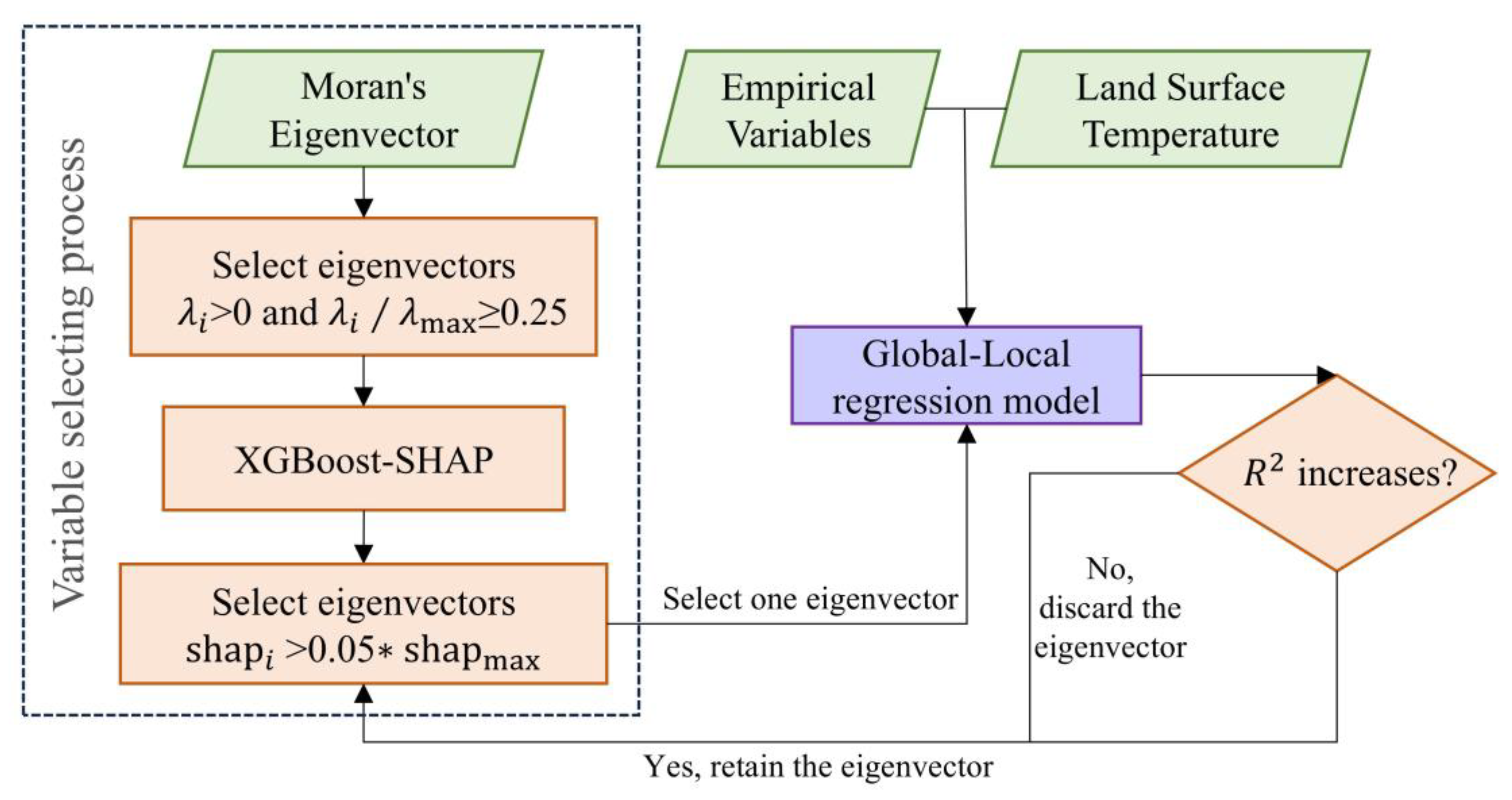
In this study, we retained only eigenvectors with eigenvalues satisfying ${\lambda }_i$ > 0 and ${\lambda }_i∕{\lambda }_{\mathrm{m}\mathrm{a}\mathrm{x}}$ ≥ 0.25 [59], where ${\lambda }_i$ denotes the eigenvalue corresponding to the $i$-th eigenvector and ${\lambda }_{\mathrm{m}\mathrm{a}\mathrm{x}}$ represents the maximum eigenvalue. The selection of Moran eigenvectors was performed by training an XGBoost model and evaluating variable contributions through SHAP analysis. We adopted those eigenvectors with SHAP values larger than 5% of the maximum SHAP value.

This variable selection method is employed to develop an efficient global–local regression (EGLR) model, which is used to estimate the surface temperature of Wuhan City. Figure 2 illustrates the research framework of this study.

4. Results

4.1. Spatial Distribution Characteristics of LST

Figure 3a presents the spatial distribution of land surface temperature (LST) of the study area in Wuhan. The maximum and minimum temperatures during the study period (August 2020) were 39.63 °C and 27.03 °C, respectively, with an average temperature of 33.21 °C and a standard deviation of 2.12 °C. The global Moran’s I value is 0.83, with a p-value significant at the 0.01 level, indicating a high level of spatial clustering of surface temperatures. Local spatial autocorrelation analysis (Figure 3b) indicates that high-high clusters are primarily distributed along both sides of the Yangtze River, predominantly involving built-up areas, including the central activity zone, residential service areas, and technology innovation zones. In contrast, the low-low clusters are predominantly distributed in the peripheral zones of the central urban area, encompassing wetland parks and urban lake systems. For example, the southern sector neighbors like Huangjia Lake Wetland Park, Tangxun Lake, and Canglong Island National Wetland Park, and the eastern sector adjoins like East Lake Ecological Tourism Scenic Area and Shahu Park, and the northern sector borders forested terrain are within relatively low-temperature areas.

4.2. Land Surface Temperature Modeling with Efficient Global–Local Regression

4.2.1. Variable Selection

A common procedure before building regression models is to test correlation and multicollinearity. The Pearson correlation analysis indicated that all explanatory variables across four major categories have strong correlation with the dependent variable (Figure A1). Additionally, variance inflation factor (VIF) values manifested the absence of multicollinearity among variables, as all VIF values were below 5 (

Table A1. OLS regression model results and VIF values.

Variable Category	Variable	Standardized Coefficient	VIF
Land use type	Water	−0.0357 **	2.076
	NDVI	−0.0074	1.850
Socioeconomic indicators	GDP	−0.0174	2.272
population	PD	0.0384	2.682
Urban form factors	ISP	0.2195 ***	3.753
	POI	0.0332	2.874
	Station	−0.0020	2.789
	RL	0.1395 ***	2.117
	BH	0.2020 ***	2.023
Natural environmental factors	DEM	0.1036 ***	1.213
	NWB	0.1713 ***	1.725
Moran’s I (error)	-	0.6363 ***	-
$R^2$	-	0.447	-

Note: ***, **, and * represent significance at the 0.001, 0.01, and 0.05 levels, respectively.

). All eleven variables under study have been selected.

The selection process of Moran eigenvectors is shown in Figure 4. First, only retain eigenvectors with eigenvalues satisfying ${\lambda }_i>0$ and ${\lambda }_i∕{\lambda }_{\mathrm{m}\mathrm{a}\mathrm{x}}\ge 0.25$. Second, put Moran eigenvectors obtained in the first step and eleven empirical variables as independent variables into the XGBoost model for fitting, then use the SHAP method to obtain the contribution value of each independent variable. Third, set 5% of the maximum SHAP value as the threshold and select the Moran eigenvectors with SHAP values exceeding this threshold. Last, take eigenvectors selected in the third step and the eleven research variables as independent variables, and use stepwise regression to gradually select the Moran eigenvectors for the GLR model. Retain eigenvectors that can improve the $R^2$ of the GLR model and remove those that cannot. In the end, seventeen Moran eigenvectors were identified through this process (

Table A2. XGBoost-SHAP-Selected Moran Eigenvectors.

Serial Number	Eigenvector Numbering	Eigenvalues	Moran’s I
1	spatial_component_1_7.9318	7.9318	0.993
27	spatial_component_27_7.4567	7.4567	0.944
148	spatial_component_148_5.7046	5.7046	0.746
16	spatial_component_16_7.6391	7.6391	0.961
60	spatial_component_60_6.9373	6.9373	0.889
35	spatial_component_35_7.3222	7.3222	0.927
11	spatial_component_11_7.7216	7.7216	0.971
21	spatial_component_21_7.5482	7.5482	0.953
4	spatial_component_4_7.8688	7.8688	0.987
7	spatial_component_7_7.8054	7.8054	0.980
36	spatial_component_36_7.2944	7.2944	0.925
9	spatial_component_9_7.7751	7.7751	0.977
29	spatial_component_29_7.4175	7.4175	0.938
42	spatial_component_42_7.2120	7.2120	0.920
3	spatial_component_3_7.8827	7.8827	0.988
78	spatial_component_78_6.6569	6.6569	0.861
100	spatial_component_100_6.3554	6.3554	0.823

). The experiments were conducted on a system running Windows 11 with Python 3.8, equipped with an Intel Core i7-13700KF processor, NVIDIA GeForce RTX 4070 Super graphics card, and 32 GB memory. For consistency and reproducibility, all subsequent experiments in this study adhered to the same hardware and software configuration.

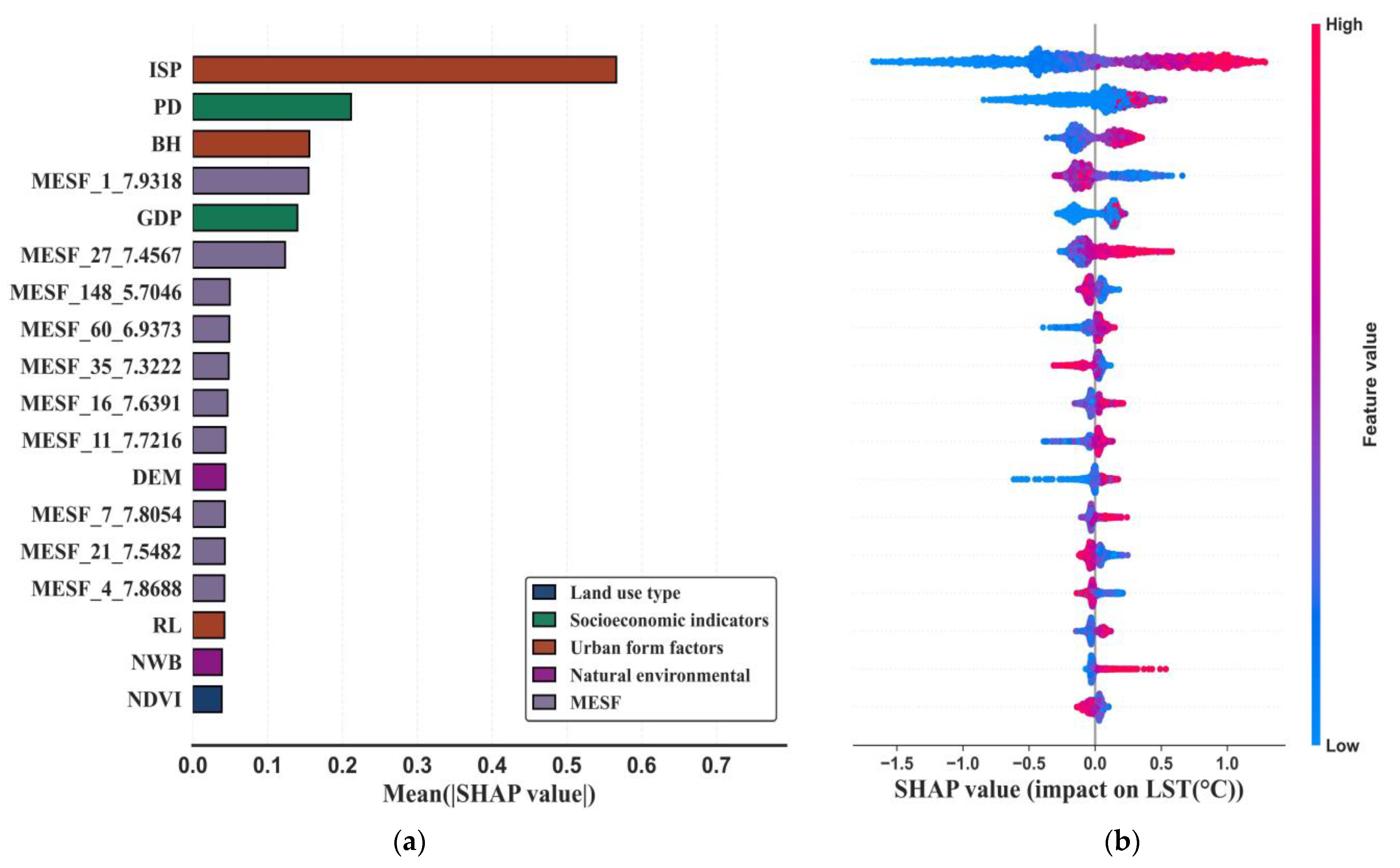
Figure 5 presents the SHAP feature importance summary plot for the influencing factors and Moran eigenvectors. Figure 5a illustrates the importance ranking of variables in relation to LST variation, ordered from the most to the least important. Figure 5b offers a local explanation of how these variables impact LST changes, visualizing the SHAP values and their directions for each variable. Here, red points represent high feature values, while blue points represent low feature values.

From Figure 5, it is evident that ISP is one of the strongest warming factors. This can be causally attributed to the high heat absorption and low emissivity of impervious surfaces, which trap more solar radiation and hinder heat dissipation, thus driving up LST. It is followed by PD and BH. Higher population density (PD) leads to more concentrated human activities, industrial operations, and waste heat release, while greater building height (BH) can disrupt air circulation and create heat-trapping urban canyons, both contributing to elevated temperatures. Then come the Moran eigenvectors, and subsequently GDP, DEM, RL, NDVI, and NWB. Urban form factors (like ISP, BH, and RL) and socioeconomic indicators (PD and GDP) exhibit the highest explanatory power for LST, which aligns with common SUHI mechanisms where urban development and economic activity reshape the thermal environment. The Moran eigenvectors also hold numerous positions, suggesting that spatial configuration—capturing the clustered or dispersed patterns of these influencing factors—has a notable explanatory effect on LST by modulating how heat is distributed across the study area. When high-value (red) points are mostly situated in the positive SHAP region, it implies that a higher value of that variable results in a greater increase in the predicted LST, as observed with ISP and BH. Conversely, when high-value (red) points are concentrated in the negative SHAP region, it indicates that higher values contribute to reducing LST, as is the case with NDVI—where lush vegetation enhances evapotranspiration and provides shading, exerting a cooling influence on the surrounding environment.

4.2.2. Model Building and Performances

As a baseline model, ordinary least squares (OLS) regression modeling was initially implemented and the GWR and MGWR models [60] were also implemented for comparison. The OLS, GWR, and MGWR models used eleven research variables, while the GLR model incorporated these eleven variables along with the Moran eigenvectors selected through forward stepwise regression. The EGLR model incorporated the same eleven research variables along with the Moran eigenvectors selected using XGBoost-SHAP procedure.

Table 3. Performance of Each Model.

Model	${\mathit{R}}^2$	MSE	Moran’s I of Residuals	Executing Time (s)
OLS	0.437	0.0159	0.630	1.4
GWR	0.876	0.0035	0.236	7.4
MGWR	0.936	0.0018	0.069	1704
GLR	0.962	0.0011	0.029	165.8
EGLR	0.961	0.0011	0.030	92.5

presents the performance of the five models. The $R^2$ of the GWR model is significantly higher than that of OLS model and the mean squared error (MSE) shows a notable decrease, indicating that the GWR model outperforms the OLS model and demonstrates significant effectiveness in capturing spatial heterogeneity. Moreover, the MGWR model further surpasses the GWR model in terms of R², while also achieving a lower MSE, suggesting that the MGWR model exhibits superior fitting performance. It is noteworthy that the GLR model demonstrates the best performance, achieving the highest R² and the lowest MSE.

In terms of computation efficiency, GWR achieved a relatively good $R^2$ value in a short amount of time, whereas MGWR took the longest time to obtain a relatively better fitting. The GLR model has the best $R^2$ value and a decent computation time. In contrast, the EGLR significantly reduces the runtime of the GLR model by up to 44.21% while maintaining nearly the same $R^2$ value. The efficient version of GLR (GLR commonly uses forward stepwise regression for variable selection, while EGLR uses XGBoost-SHAP for variable selection; the difference between GLR and EGLR is that the latter employs XGBoost-SHAP to choose variables), that is EGLR, achieved the best fitting with relatively short time, indicating that the method of selecting Moran eigenvectors using XGBoost-SHAP values is helpful to improve the operational efficiency of the GLR model.

4.2.3. Relationship Between Driving Factors and LST

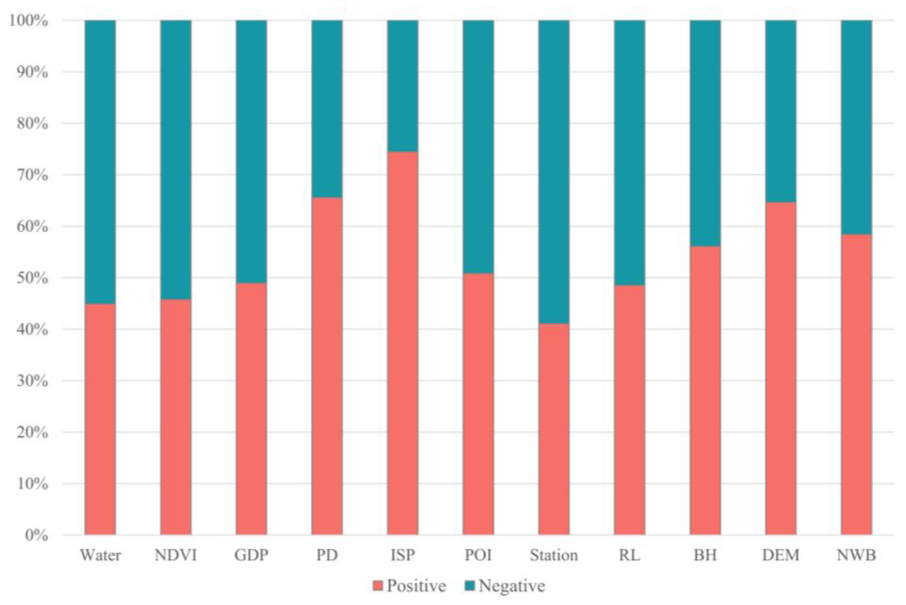
Figure 6 illustrates the proportions of positive and negative influences of eleven variables on land surface temperature (LST) in EGLR model. Among them, population density (PD), impervious surface area (ISP), building height (BH), elevation (DEM), and distance to the nearest water body (NWB) mainly exhibit positive effects on LST, with the influence proportions reaching 65.59%, 74.46%, 56.11%, 64.65%, and 58.42%, respectively. In contrast, water area (Water), normalized difference vegetation index (NDVI), and the number of bus stops (Station) show negative effects on LST, with the influence proportions reaching 55.07%, 54.21%, and 58.91%, respectively. The positive and negative influence proportions of the number of points of interest (POI), gross domestic product (GDP), and road length (RL) are almost equal.

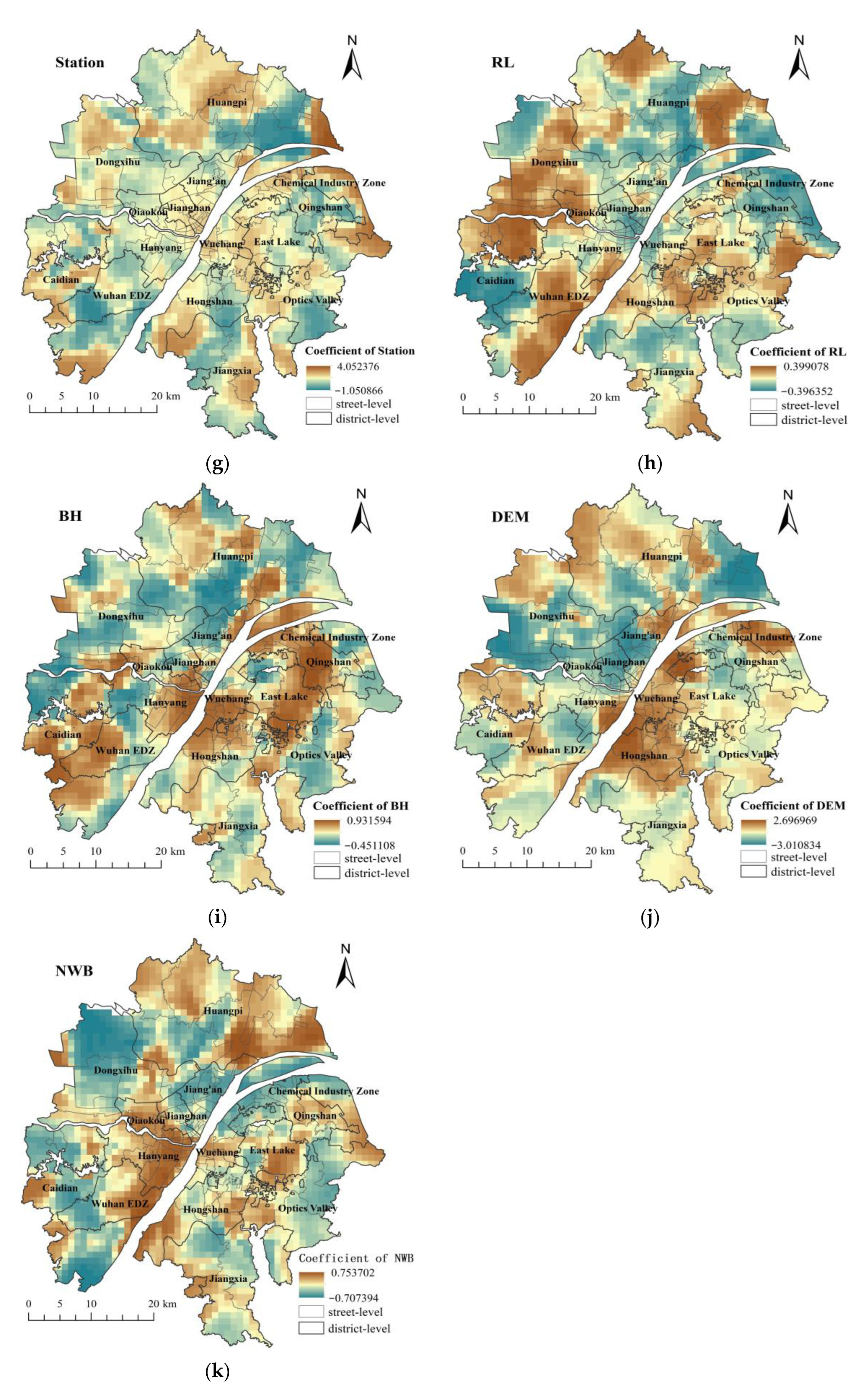
Figure 7 illustrates the spatial differentiation characteristics of the coefficients of each influencing factor in the EGLR model. In the following maps, red areas represent that the factor has a significant positive effect on the land surface temperature (LST), green areas indicate a significant negative effect, and yellow areas suggest that no statistically significant correlation has been detected.

(1)

Spatial impacts of land use type on LST

For the land use type factors, both percentage of water area (Water) and NDVI show significant spatial non-stationarity (Figure 7a,b). The mean coefficient of the percentage of water body is −0.019, indicating a weak negative correlation to LST. However, coefficients in local areas tell a different story. Negative correlation coefficients can be observed in the southern part of Huangpi District, the eastern and northern parts of Dongxihu District, Hanyang District, and the East Lake area, as well as along the edges of the study region. These areas are rich in water bodies, whose high specific heat capacity slows the rate of temperature increase and helps regulate the local microclimate [61,62]. Through these mechanisms, water bodies absorb heat during the day and release it at night, effectively lowering the surrounding environmental temperature. Unexpectedly, however, Jiang’an District, Jianghan District, and Wuchang District, located on both banks of the Yangtze River and likewise endowed with abundant water resources, exhibit positive correlation coefficients. In some water areas, an “urban heat bath” effect appears (Figure 7a). This phenomenon may be associated with high building density around lakes and deteriorating ventilation conditions. Brans et al. [63] reported that the impact of urbanization within a radius of 50 m on lake water temperature was much larger than the impact of urbanization in the vicinity of 3200 m.

The impact of the NDVI on LST is generally negative [64], however, in certain urban center areas of Wuhan, NDVI is positively correlated with LST. Under extreme heat conditions, this phenomenon may be related to differences between dry-heat and moist-heat characteristics within the region. The cooling capacity of vegetation varies markedly across urban functional zones: it is lowest in commercial areas and highest in green spaces [65]. In addition, this disparity may be influenced by vegetation type. For example, shorter vegetation (such as lawns and shrubs) has a limited effect in mitigating adverse thermal conditions in the surrounding environment [66,67]; by contrast, tree height, the height of surrounding buildings, and the shade provided by the canopy jointly constitute key factors in regulating surface temperature [68].

(2)

Spatial impacts of socioeconomic indicators on LST

The impacts of GDP also exhibit significant spatial non-stationarity (Figure 7c). In central areas where the economy is more developed, the impact of GDP on surface temperature is relatively smaller. In contrast, the surrounding areas exhibit clustered negative and positive effects. This phenomenon may be related to local industrial structures. For example, in service- and high technology-oriented areas (such as Jianghan, Wuchang, Jiang’an, and Qiaokou), industries centered on finance, commerce, and the digital economy are characterized by low pollution and low energy consumption [69,70]. Through the adoption of clean energy, improvements in energy efficiency, and optimization of production processes, these areas reduce sensible and waste heat emissions. Consequently, during economic expansion, the incremental increases in greenhouse gas emissions and residual heat are relatively small, resulting in a weaker elevating effect on land surface temperature. In contrast, industrially dominated areas such as Qingshan District, Dongxihu District, and Optics Valley agglomerate energy-intensive or heavy industries, including automobile manufacturing, steel and petrochemical supporting sectors, and new energy industries. Their industrial processes and equipment operation release large amounts of residual heat, markedly driving local air temperature increases.

The mean coefficient of population density (PD) is 0.373, indicating that PD is positively correlated to LST. However, being similar to GDP, population density also exhibits significant spatial non-stationarity. Population density in the central area has a relatively smaller impact on LST, while population density in the surrounding areas have greater influences on LST. The warming effect is mainly concentrated in the southwestern regions such as Huangpi and Economic and Technological Development Zone (ETDZ), while the cooling effect is primarily observed in Dongxihu and the northeastern part of the study area (Figure 7d). This phenomenon may stem from the fact that the central urban area is already highly urbanized: buildings are densely packed and permeable surfaces and vegetated patches are scarce, so the UHI has long been in a near “saturated” state. Under these conditions, further increases in population density produce only limited marginal changes in the composition and physical properties of the underlying surface, making it difficult to induce a substantial additional rise in land surface temperature. In contrast, the peripheral zones were originally dominated by farmland and natural surfaces; rising population density there is often accompanied by land-use conversion to built-up uses, with large increases in impervious, low-albedo and/or high heat-storage artificial materials, thereby intensifying surface warming. Moreover, given the relatively strong industrial base of the peripheral areas, higher population density may also signal the introduction or expansion of energy-intensive production facilities and ancillary equipment, further amplifying anthropogenic waste heat emissions and local warming effects.

(3)

Spatial impacts of urban form factors on LST

Among the urban form factors, impervious surface area (ISP) shows a significant positive correlation with LST in central areas such as Jiang’an, Wuchang, and Qingshan, where the high coverage of impervious surfaces leads to intensive heat accumulation, thus driving up LST. However, as depicted in Figure 7e, it turns into negative in the East Lake Area. In this region, the combined effect of the lake’s cooling influence and the relatively optimized spatial configuration counteracts the typical warming effect of ISP, resulting in a negative correlation with LST.

The relationship between POI and LST shows a distinct spatial differentiation pattern exhibits a pronounced spatial differentiation pattern characterized by two types of extreme patches: a strongly negative correlation, spanning Dongxihu and eastern Huangpi, and a strongly positive-correlation high-value zone, covering the Economic and Technological Development Zone (ETDZ) and the main body of Huangpi District. Beyond these zones, the remaining areas are dotted with multi-level positive and negative correlation patches of varying intensity, forming a fragmented pattern (Figure 7f).

Similarly, the relationship between the number of bus stops (Station) and land surface temperature shows pronounced spatial heterogeneity, with the region interwoven by positive and negative correlation patches of differing intensity in a multi-level, highly fragmented pattern (Figure 7g).

Road length (RL) exerts a predominantly positive influence on LST (Figure 7h), with hotspots mainly located in Dongxihu District, northern Caidian District, the ETDZ, and the junction area of East Lake, Optics Valley, and Hongshan District. The likely mechanism is that a high proportion of artificial impervious surfaces, with relatively large heat capacity and thermal conductivity, lowers surface albedo and enhances the absorption of solar radiation, thereby intensifying warming. The negative effects are mainly concentrated in the Chemical Industry Zone, Qingshan District, the southern part of Caidian District, and Huangpi District. This may be because these areas are dominated by farmland, wetlands/marshes, and water bodies, which weaken the surface RL warming effect and can even produce a net cooling effect.

Building height (BH) also exerts a significant influence on LST (Figure 7i). Positive correlations can be observed in Hanyang, Wuchang, Hongshan, Caidian, the ETDZ, East Lake, and Qingshan, likely because taller buildings and high-density urban morphology impede air circulation and reduce near-surface wind speed, thereby intensifying the SUHI effect [71]. In contrast, BH are negatively correlated with LST in peripheral urban areas.

(4)

Spatial impacts of natural environmental on LST

In terms of natural environmental factors, the digital elevation model (DEM) primarily exerts a positive influence on land surface temperature (LST). The regions with significant positive impacts are concentrated in Hongshan, Wuchang, and the Chemical Industry Zone. Within these areas, higher elevations may give rise to specific microclimatic conditions, such as diminished heat dissipation or modified solar radiation reception, which consequently contribute to elevated LST. Meanwhile, the areas with negative low values mainly occur in Huangpi, Qiaokou, Jianghan, and Jiang’an (Figure 7j). In these regions with negative impacts, lower elevations might be correlated with superior air circulation or other temperature-mitigating factors, leading to a negative correlation with LST.

NWB exhibits pronounced spatial non-stationarity. Regions including the Economic and Technological Development Zone (ETDZ) and Hanyang present positive coefficients. As illustrated in Figure 7k, the proximity to water bodies in these areas, in conjunction with urban development patterns, is likely to amplify the positive impact on LST. In contrast, Jiang’an and Qingshan show negative coefficients. Furthermore, areas that are far from water bodies or close to water but remote from the urban center, such as parts of Huangpi, tend to have negative values. This may be attributed to the fact that in these less urbanized or more distant regions, the cooling effect of water might be less significant or counteracted by other factors. On the other hand, zones adjacent to water bodies and near the urban center, like the vicinity of East Lake, display positive values. This is potentially due to the combined effect of urban heat and the intricate interaction between water and built environments in central areas.

5. Discussion

This section examines the role of the proposed Moran eigenvector selecting method in enhancing computational efficiency from multiple perspectives. First, we independently compare the selection efficiency of the forward stepwise regression method versus the proposed XGBoost-SHAP method for Moran eigenvectors. Second, we assess the performance of the GLR model under different sample sizes when using the classical versus the proposed selection strategy. Finally, we investigate how extending the EGLR framework to machine learning models improves their performance.

5.1. Computational Efficiency Comparison Between XGBoost-SHAP and Forward Stepwise Regressive Selecting for Moran Eigenvectors

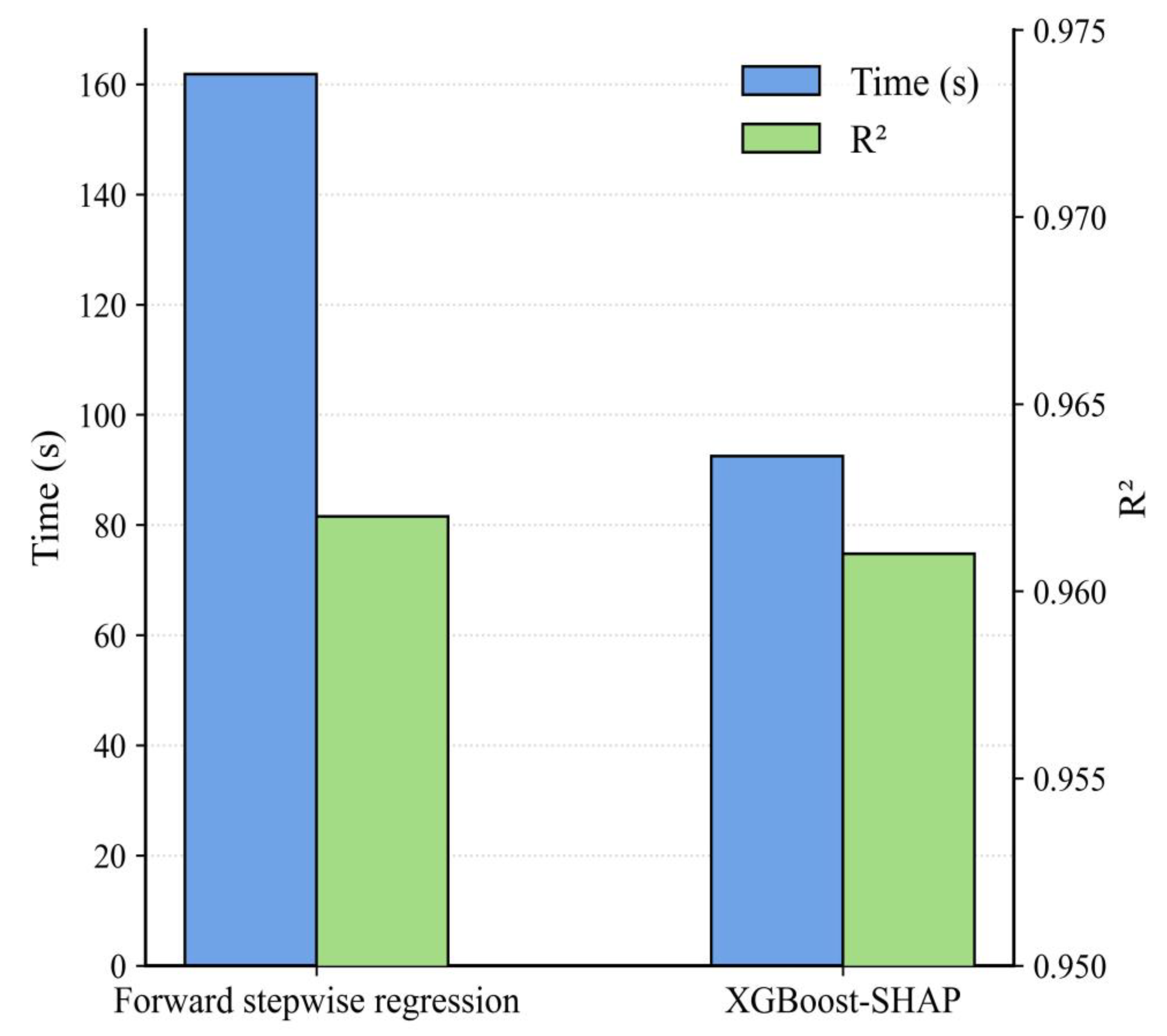
To separately evaluate the efficiency gains in feature selection afforded by the XGBoost-SHAP method, we designed the following experiment.

In the experiments, we uniformly defined the independent variables as the eleven factors influencing land surface temperature, along with the eigenvectors whose eigenvalues satisfy ${\lambda }_i>0$ and ${\lambda }_i∕{\lambda }_{\mathrm{m}\mathrm{a}\mathrm{x}}\ge 0.25$. In Experiment 1, variable selection was carried out using the forward selection method applied in the GLR model. In Experiment 2, variable selection was performed using the XGBoost-SHAP value method employed in the innovative EGLR model proposed in this study.

The results, as shown in Figure 8, indicate that the method utilizing XGBoost-SHAP achieves a substantial reduction in computation time at the expense of only a slight decrease in $R^2$.

5.2. XGBoost-SHAP Selecting for Moran Eigenvectors on Different Sample Sizes

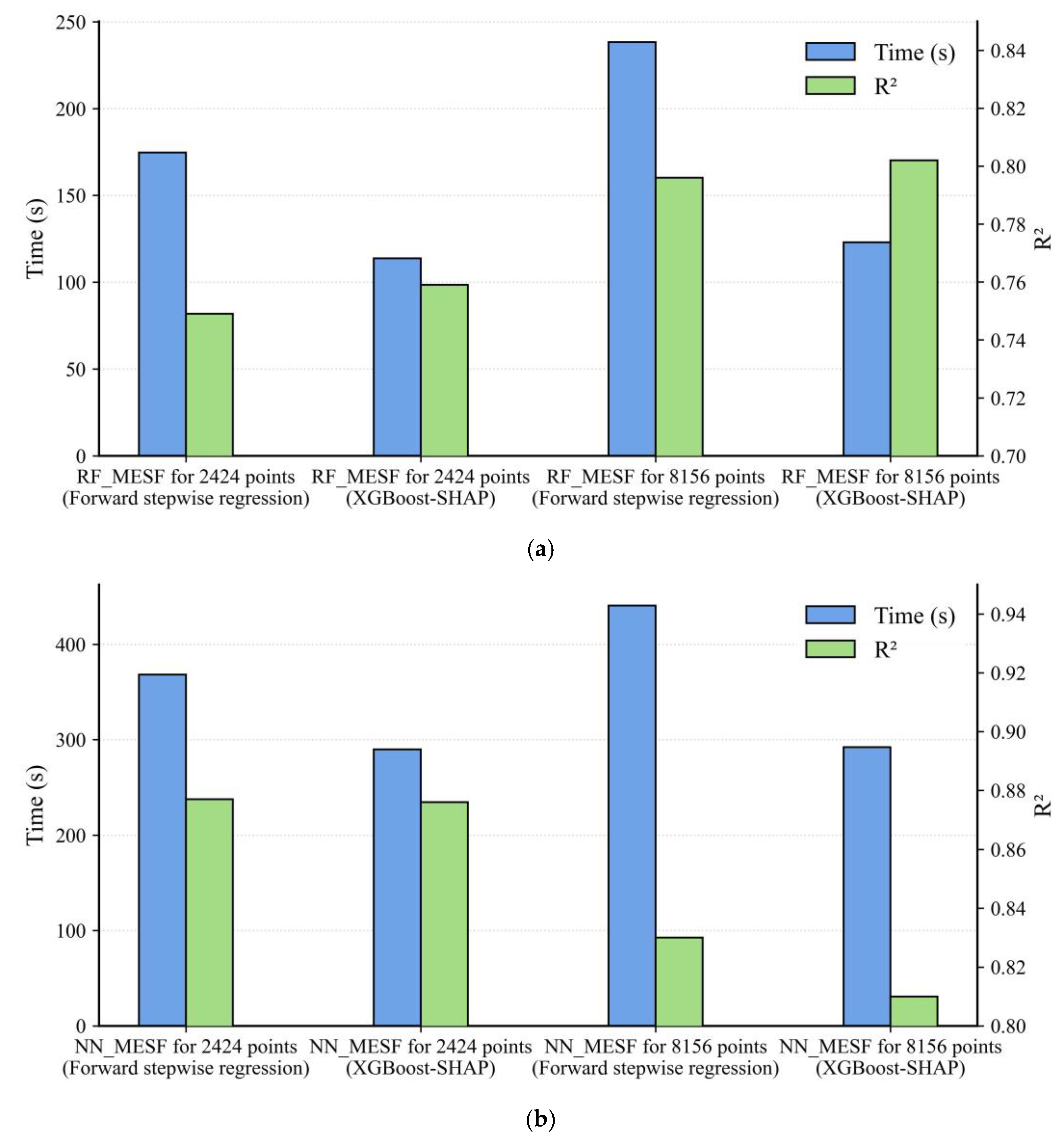
We also evaluated the model performances of GLR and EGLR for different sample sizes (Figure 9). The first sample consists of 2424 data points, representing the relatively central area of Wuhan (the study area of SUHI of this study), while the second sample includes 8156 data points, covering the entire city of Wuhan. In the experiment, we consistently selected eleven factors influencing land surface temperature as independent variables. These factors were chosen based on their eigenvalues and eigenvectors, satisfying the criteria ${\lambda }_i>0$ and ${\lambda }_i∕{\lambda }_{\mathrm{m}\mathrm{a}\mathrm{x}}\ge 0.25$. The GLR uses forward stepwise regression for variable selecting, while the EGLR employs the XGBoost-SHAP method. As shown in Figure 9, the GLR equipped with XGBoost-SHAP approach (i.e., the EGLR) cost less than 60% computational time of GLR for both 2424 and 8156 sample sizes, and the EGLR maintained nearly the same $R^2$ as GLR. When the sample size increases, the computation time for GLR rises by approximately 115.6%, while EGLR experiences an increase of about 115.8%. This indicates that while EGLR demonstrates exceptional performance in smaller sample sizes, its computational efficiency remains robust even as the sample size grows, maintaining its reliability and effectiveness in handling larger datasets.

5.3. Expanding EGLR Framework to Two Machine Learning Models

In thermal environment studies, some scholars have employed machine learning approaches such as random forest (RF) and neural networks (NN) [27]. To validate the applicability of the proposed efficient feature selecting framework, we incorporated the proposed EGLR concept into both RF and NN methodologies (Figure 10), in which both empirical variables and Moran eigenvectors are included as input features.

We compared model performances of traditional random forest (RF) and neural network (NN) models and their new versions with Moran eigenvectors (RF_MESF and NN_MESF, respectively). For RF_MESF and NN_MESF, the XGBoost-SHAP feature selection method was employed. The results are shown in

Table 4. Performance of machine learning models.

Model	${\mathit{R}}^2$	MSE	Time (s)
RF	0.521	0.0135	3.5
RF_MESF	0.759	0.0068	113.8
NN	0.433	0.0157	19.4
NN_MSEF	0.876	0.0036	289.68

. Although the execution efficiency of the Moran eigenvector versions is much slower than traditional RF and NN, the $R^2$ improves a lot, with increases by 45.68% and 102.31% for RF and NN, respectively.

In addition, the model performances of RF_MESF and NN_MESF equipped with forward regressive variable selection and XGBoost-SHAP variable selection for different sample sizes were evaluated. It can be seen from Figure 11 that RF_MESF and NN_MESF equipped with the XGBoost-SHAP method still maintain almost the same $R^2$ as those using forward stepwise regressive selecting procedure, but the former methods save a significant amount of running time.

In conclusion, the experimental results demonstrate that the XGBoost-SHAP method exhibits significant execution efficiency advantages over traditional forward stepwise regression across different sample sizes. Specifically, with a sample size of 2424, the EGLR model achieves the most prominent improvement in efficiency, reaching 44.21% (Figure 9), while the RF_MESF and NN_MESF models achieve time optimizations of 34.85% and 21.31%, respectively (Figure 11a,b). When the sample size increases to 8156, the RF_MSEF with XGBoost-SHAP demonstrates impressive time performance, reducing computation time by 48.39% (Figure 11a), while the GLR and NN_MESF models achieve time efficiency improvements of 39.89% (Figure 9) and 33.68% (Figure 11b), respectively. This indicates that the XGBoost-SHAP based selection of Moran eigenvectors yields a more pronounced improvement in runtime efficiency on datasets with large sample sizes.

5.4. Limitations

However, it is worth noting that the EGLR framework model has certain limitations. For instance, how to select an appropriate number of Moran eigenvectors after obtaining the feature importance ranking through the SHAP value method is a question worthy of consideration. Additionally, how dealing with situations where the fitting effect of the XGBoost model is extremely poor is also a problem that merits thought.

6. Conclusions

This study proposes a computationally efficient version of the global–local regression model (i.e., EGLR) by employing the XGBoost-SHAP method to accelerating variables selecting procedure. Experiments have shown that the EGLR reduces execution time by 44.21% while maintaining $R^2$. The results of EGLR also indicate spatial heterogeneity in the impacts of driving factors on LST.

Among the explanatory variables, population density (PD) exhibits the highest sensitivity to LST, showing a positive effect in 65.59% of the study units. Additionally, population density (PD) has the largest mean coefficient of 0.373. The impervious surface area (ISP), building height (BH), elevation (DEM), and distance to the nearest water body (NWB) exhibit positive influences across more than 50% of the study units. Conversely, water area (Water), normalized difference vegetation index (NDVI), and the number of bus stops (Station) show negative influences in more than 50% units. The number of points of interest (POI), gross domestic product (GDP), and road length (RL) present relatively balanced positive and negative influences. Variables with a positive impact on LST are typically associated with densely built-up areas along both sides of the Yangtze River, while variables with a negative impact on LST are generally linked to areas farther from the city center with lower building density.

These conclusions have several implications for mitigating SUHI effects. For example, in densely built urban centers where space is limited and large-scale greening is challenging, vertical greening, increased vegetation density, and the selection of appropriate plant species can be implemented. Additionally, optimizing building heights and spatial distribution to improve air circulation can effectively reduce temperatures. Furthermore, the study highlights that water bodies exhibit excellent negative effects, even surpassing those of vegetation. Given Wuhan’s abundant water resources, the rational utilization of water bodies—such as constructing parks, wetlands, and ponds near schools or factories—can play a more active role in temperature reduction [72]. Beyond these measures, enhancing energy efficiency, adopting clean energy to reduce anthropogenic heat emissions, and raising public environmental awareness to promote energy-saving policies and green lifestyles will contribute to mitigating the adverse effects of the SUHI phenomenon.

The computation efficiency of EGLR and machine learning models equipped with the EGLR framework (i.e., integrating the XGBoost-SHAP procedure and MESF) were also discussed, and we obtained following conclusions:

(1)

The XGBoost-SHAP method significantly reduces the time required for selecting Moran eigenvectors compared to the traditional forward stepwise regressive selecting procedure.

(2)

For datasets with a large sample size, the XGBoost-SHAP method still achieves significant computational time savings compared to the forward stepwise regressive selecting procedure.

(3)

The integrated XGBoost-SHAP process and MESF are also applicable to machine learning methods, significantly improving the R² of RF and NN models with acceptable running time.

In summary, the proposed efficient global–local regression (EGLR) framework integrates the XGBoost-SHAP method into statistical modeling, retaining model interpretability while significantly enhancing computational efficiency. Notably, beyond computational gains, both neural networks and random forest models exhibit substantial performance improvements. This demonstrates the significant potential of integrating spatial features with machine learning methodologies. As we enter the era of geographical artificial intelligence (GeoAI), future research may further explore synergistic integrations of machine learning and statistical models to achieve high computational efficiency, robust predictive performance, and enhanced interpretability.

References

1. Oke, T.R. City Size and the Urban Heat Island. Atmos. Environ. 1973, 7, 769–779. [Google Scholar] [CrossRef]
2. Zhao, L.; Lee, X.; Smith, R.B.; Oleson, K. Strong contributions of local background climate to urban heat islands. Nature 2014, 511, 216–219. [Google Scholar] [CrossRef] [PubMed]
3. Waha, K.; Krummenauer, L.; Adams, S.; Aich, V.; Baarsch, F.; Coumou, D.; Fader, M.; Hoff, H.; Jobbins, G.; Marcus, R.; et al. Climate change impacts in the Middle East and Northern Africa (MENA) region and their implications for vulnerable population groups. Reg. Environ. Change 2017, 17, 1623–1638. [Google Scholar] [CrossRef]
4. Founda, D.; Santamouris, M. Synergies between Urban Heat Island and Heat Waves in Athens (Greece), during an extremely hot summer (2012). Sci. Rep. 2017, 7, 10973. [Google Scholar] [CrossRef]
5. Qian, Y.; Chakraborty, T.C.; Li, J.; Li, D.; He, C.; Sarangi, C.; Chen, F.; Yang, X.; Leung, L.R. Urbanization Impact on Regional Climate and Extreme Weather: Current Understanding, Uncertainties, and Future Research Directions. Adv. Atmos. Sci. 2022, 39, 819–860. [Google Scholar] [CrossRef]
6. Ginzburg, A.S.; Dokukin, S.A. Influence of Thermal Air Pollution on the Urban Climate (Estimates Using the COSMO-CLM Model). Izv. Atmos. Ocean. Phys. 2021, 57, 47–59. [Google Scholar] [CrossRef]
7. Klimenko, V.V.; Ginzburg, A.S.; Demchenko, P.F.; Tereshin, A.G.; Belova, I.N.; Kasilova, E.V. Impact of urbanization and climate warming on energy consumption in large cities. Dokl. Phys. 2016, 61, 521–525. [Google Scholar] [CrossRef]
8. Souza, F.L.; Puppim de Oliveira, J.A.; Lepczyk, C.A. Editorial: Urban Ecosystem Services and Disservices in Tropical Regions. Front. Ecol. Evol. 2021, 9, 791070. [Google Scholar] [CrossRef]
9. Lee, Y.Y.; Din, M.F.M.; Ponraj, M.; Noor, Z.Z.; Iwao, K.; Chelliapan, S. Overview of Urban Heat Island (UHI) phenomenon towards human thermal comfort. Environ. Eng. Manag. J. 2017, 16, 2097–2111. [Google Scholar] [CrossRef]
10. Song, J.; Yu, H.; Lu, Y. Spatial-scale dependent risk factors of heat-related mortality: A multiscale geographically weighted regression analysis. Sustain. Cities Soc. 2021, 74, 103159. [Google Scholar] [CrossRef]
11. Guo, Y.; Li, S.; Liu, D.L.; Chen, D.; Williams, G.; Tong, S. Projecting future temperature-related mortality in three largest Australian cities. Environ. Pollut. 2016, 208, 66–73. [Google Scholar] [CrossRef] [PubMed]
12. Voogt, J.A.; Oke, T.R. Thermal remote sensing of urban climates. Remote Sens. Environ. 2003, 86, 370–384. [Google Scholar] [CrossRef]
13. Ali, J.M. Modelling the Spatiotemporal Change of Urban Heat Islands and Influencing Parameters. Ph.D. Thesis, University of Nottingham, Nottingham, UK, 2017. [Google Scholar]
14. Cai, J.; Tan, W.; Yan, B. The Structure of Urban Green Space System to tackle Heat-island Effect. Res. J. Chem. Environ. 2011, 15, 755–758. [Google Scholar]
15. Carpio, M.; Gonzalez, A.; Gonzalez, M.; Verichev, K. Influence of pavements on the urban heat island phenomenon: A scientific evolution analysis. Energy Build. 2020, 226, 110379. [Google Scholar] [CrossRef]
16. Mohajerani, A.; Bakaric, J.; Jeffrey-Bailey, T. The urban heat island effect, its causes, and mitigation, with reference to the thermal properties of asphalt concrete. J. Environ. Manag. 2017, 197, 522–538. [Google Scholar] [CrossRef]
17. Ward, K.; Lauf, S.; Kleinschmit, B.; Endlicher, W. Heat waves and urban heat islands in Europe: A review of relevant drivers. Sci. Total Environ. 2016, 569, 527–539. [Google Scholar] [CrossRef]
18. Ban, Y.; Liu, X.; Yin, Z.; Li, X.; Yin, L.; Zheng, W. Effect of urbanization on aerosol optical depth over Beijing: Land use and surface temperature analysis. Urban Clim. 2023, 51, 101655. [Google Scholar] [CrossRef]
19. Qiao, Z.; He, T.; Wang, N.; Wu, F.; Chen, J.; Xu, X.; Liu, L.; Zhang, Q. How Do Natural Factor and Human Activity Affect Urban Land Surface Heat Environment in China? Ecosyst. Health Sustain. 2023, 9, 0126. [Google Scholar] [CrossRef]
20. Wang, H.; Zhang, Y.; Tsou, J.Y.; Li, Y. Surface Urban Heat Island Analysis of Shanghai (China) Based on the Change of Land Use and Land Cover. Sustainability 2017, 9, 1538. [Google Scholar] [CrossRef]
21. Yu, M.; Chen, X.; Yang, J.; Miao, S. A new perspective on evaluating high-resolution urban climate simulation with urban canopy parameters. Urban Clim. 2021, 38, 100919. [Google Scholar] [CrossRef]
22. Kusaka, H.; Chen, F.; Tewari, M.; Dudhia, J.; Gill, D.O.; Duda, M.G.; Wang, W.; Miya, Y. Numerical Simulation of Urban Heat Island Effect by the WRF Model with 4-km Grid Increment: An Inter-Comparison Study between the Urban Canopy Model and Slab Model. J. Meteorol. Soc. Jpn. 2012, 90, 33–45. [Google Scholar] [CrossRef]
23. Byon, J.Y.; Choi, Y.J.; Seo, B.G. Evaluation of Urban Weather Forecast Using WRF-UCM (Urban Canopy Model) Over Seoul. Atmosphere 2010, 20, 13–26. [Google Scholar]
24. Guo, A.; Yang, J.; Xiao, X.; Xia, J.; Jin, C.; Li, X. Influences of urban spatial form on urban heat island effects at the community level in China. Sustain. Cities Soc. 2020, 53, 101972. [Google Scholar] [CrossRef]
25. Shahfahad; Naikoo, M.W.; Islam, A.R.M.T.; Mallick, J.; Rahman, A. Land use/land cover change and its impact on surface urban heat island and urban thermal comfort in a metropolitan city. Urban Clim. 2022, 41, 101052. [Google Scholar] [CrossRef]
26. Yang, L.; Yu, K.; Ai, J.; Liu, Y.; Yang, W.; Liu, J. Dominant Factors and Spatial Heterogeneity of Land Surface Temperatures in Urban Areas: A Case Study in Fuzhou, China. Remote Sens. 2022, 14, 1266. [Google Scholar] [CrossRef]
27. Gao, Y.; Li, N.; Gao, M.; Hao, M.; Liu, X. Modelling Future Land Surface Temperature: A Comparative Analysis between Parametric and Non-Parametric Methods. Sustainability 2024, 16, 8195. [Google Scholar] [CrossRef]
28. Zhang, G.P. Time series forecasting using a hybrid ARIMA and neural network model. Neurocomputing 2003, 50, 159–175. [Google Scholar] [CrossRef]
29. Jia, S.; Wang, Y.; Ling, C.; Bi, X. A novel approach to estimating urban land surface temperature by the combination of geographically weighted regression and deep neural network models. Urban Clim. 2023, 47, 101390. [Google Scholar] [CrossRef]
30. Hagenauer, J.; Helbich, M. A geographically weighted artificial neural network. Int. J. Geogr. Inf. Sci. 2022, 36, 215–235. [Google Scholar] [CrossRef]
31. Du, Z.; Wang, Z.; Wu, S.; Zhang, F.; Liu, R. Geographically neural network weighted regression for the accurate estimation of spatial non-stationarity. Int. J. Geogr. Inf. Sci. 2020, 34, 1353–1377. [Google Scholar] [CrossRef]
32. Su, H.; Chen, Y.; Tan, H.; Zhou, A.; Chen, G.; Chen, Y. Estimating Regional PM2.5 Concentrations in China Using a Global-Local Regression Model Considering Global Spatial Autocorrelation and Local Spatial Heterogeneity. Remote Sens. 2022, 14, 4545. [Google Scholar] [CrossRef]
33. Brunsdon, C.; Fotheringham, A.S.; Charlton, M.E. Geographically Weighted Regression: A Method for Exploring Spatial Nonstationarity. Geogr. Anal. 1996, 28, 281–298. [Google Scholar] [CrossRef]
34. Getis, A.; Griffith, D.A. Comparative Spatial Filtering in Regression Analysis. Geogr. Anal. 2002, 34, 130–140. [Google Scholar] [CrossRef]
35. Peel, M.C.; Finlayson, B.L.; McMahon, T.A. Updated world map of the Köppen-Geiger climate classification. Hydrol. Earth Syst. Sci. 2007, 11, 1633–1644. [Google Scholar] [CrossRef]
36. Zhou, X.; Chen, H. Impact of urbanization-related land use land cover changes and urban morphology changes on the urban heat island phenomenon. Sci. Total Environ. 2018, 635, 1467–1476. [Google Scholar] [CrossRef]
37. Gui, X.; Wang, L.; Yao, R.; Yu, D.; Li, C.A. Investigating the urbanization process and its impact on vegetation change and urban heat island in Wuhan, China. Environ. Sci. Pollut. Res. 2019, 26, 30808–30825. [Google Scholar] [CrossRef] [PubMed]
38. Zhao, Z.Q.; He, B.J.; Li, L.G.; Wang, H.B.; Darko, A. Profile and concentric zonal analysis of relationships between land use/land cover and land surface temperature: Case study of Shenyang, China. Energy Build. 2017, 155, 282–295. [Google Scholar] [CrossRef]
39. Oliver, L.N.; Schuurman, N.; Hall, A.W. Comparing circular and network buffers to examine the influence of land use on walking for leisure and errands. Int. J. Health Geogr. 2007, 6, 41. [Google Scholar] [CrossRef] [PubMed]
40. Li, Y.; Sun, Y.; Li, J.; Gao, C. Socioeconomic drivers of urban heat island effect: Empirical evidence from major Chinese cities. Sustain. Cities Soc. 2020, 63, 102425. [Google Scholar] [CrossRef]
41. Xi, Y.; Wang, S.; Zou, Y.; Zhou, X.; Zhang, Y. Seasonal surface urban heat island analysis based on local climate zones. Ecol. Indic. 2024, 159, 111669. [Google Scholar] [CrossRef]
42. Mashhoodi, B.; Unceta, P.M. Urban form and surface temperature inequality in 683 European cities. Sustain. Cities Soc. 2024, 113, 105690. [Google Scholar] [CrossRef]
43. Zhang, X.; Zhao, T.; Xu, H.; Liu, W.; Wang, J.; Chen, X.; Liu, L. GLC_FCS30D: The first global 30 m land-cover dynamics monitoring product with a fine classification system for the period from 1985 to 2022 generated using dense-time-series Landsat imagery and the continuous change-detection method. Earth Syst. Sci. Data 2024, 16, 1353–1381. [Google Scholar] [CrossRef]
44. Zhao, N.; Liu, Y.; Cao, G.; Samson, E.L.; Zhang, J. Forecasting China’s GDP at the pixel level using nighttime lights time series and population images. GISci. Remote Sens. 2017, 54, 407–425. [Google Scholar] [CrossRef]
45. Che, Y.; Li, X.; Liu, X.; Wang, Y.; Liao, W.; Zheng, X.; Zhang, X.; Xu, X.; Shi, Q.; Zhu, J.; et al. 3D-GloBFP: The first global three-dimensional building footprint dataset. Earth Syst. Sci. Data 2024, 16, 5357–5374. [Google Scholar] [CrossRef]
46. Delgado, R.C.; de Oliveira-Junior, J.F.; Gois, G.; Rodrigues, R.d.A.; Teodoro, P.E. Synoptic events associated with the land surface temperature in Rio de Janeiro. Biosci. J. 2017, 33, 1038–1047. [Google Scholar] [CrossRef]
47. Moran, P.A. Notes on continuous stochastic phenomena. Biometrika 1950, 37, 17–23. [Google Scholar] [CrossRef]
48. Amelin, L. Local Indicators of Spatial Association-LISA. Geogr. Anal. 1995, 27, 93–115. [Google Scholar]
49. Chun, Y.; Griffith, D.A. A quality assessment of eigenvector spatial filtering based parameter estimates for the normal probability model. Spat. Stat. 2014, 10, 1–11. [Google Scholar] [CrossRef]
50. Chun, Y.; Griffith, D.A.; Lee, M.; Sinha, P. Eigenvector selection with stepwise regression techniques to construct eigenvector spatial filters. J. Geogr. Syst. 2016, 18, 67–85. [Google Scholar] [CrossRef]
51. Yu, Z.; Yu, R.; Ge, X.; Fu, J.; Hu, Y.; Chen, S. Tabular prior-data fitted network for urban air temperature inference and high temperature risk assessment. Sustain. Cities Soc. 2025, 128, 106484. [Google Scholar] [CrossRef]
52. Joharestani, M.Z.; Cao, C.; Ni, X.; Bashir, B.; Talebiesfandarani, S. PM2.5 Prediction Based on Random Forest, XGBoost, and Deep Learning Using Multisource Remote Sensing Data. Atmosphere 2019, 10, 373. [Google Scholar] [CrossRef]
53. Chen, T.; Guestrin, C. XGBoost: A Scalable Tree Boosting System. In Proceedings of the 22nd ACM SIGKDD International Conference on Knowledge Discovery and Data Mining, San Francisco, CA, USA, 13–17 August 2016. [Google Scholar]
54. Meddage, D.P.P.; Ekanayake, I.U.; Weerasuriya, A.U.; Lewangamage, C.S.; Tse, K.T.; Miyanawala, T.P.; Ramanayaka, C.D.E. Explainable Machine Learning (XML) to predict external wind pressure of a low-rise building in urban-like settings. J. Wind Eng. Ind. Aerodyn. 2022, 226, 105027. [Google Scholar] [CrossRef]
55. Lundberg, S. Explainable Machine Learning for Science and Medicine. Ph.D. Thesis, University of Washington, Seattle, WA, USA, 2019. [Google Scholar]
56. Mo, T.; Li, S.; Li, G. An interpretable machine learning model for predicting cavity water depth and cavity length based on XGBoost-SHAP. J. Hydroinform. 2023, 25, 1488–1500. [Google Scholar] [CrossRef]
57. Liao, J.; Wang, L.; Duan, L.; Gong, F.; Zhu, H.; Pan, H.; Yang, H. Association between estimated glucose disposal rate and cardiovascular diseases in patients with diabetes or prediabetes: A cross-sectional study. Cardiovasc. Diabetol. 2025, 24, 13. [Google Scholar] [CrossRef]
58. Gu, X.; Wu, Z.; Liu, X.; Qiao, R.; Jiang, Q. Exploring the Nonlinear Interplay between Urban Morphology and Nighttime Thermal Environment. Sustain. Cities Soc. 2024, 101, 105176. [Google Scholar] [CrossRef]
59. Griffith, D.A.; Paelinck, J.H.P. Non-Standard Spatial Statistics and Spatial Econometrics; Springer: Berlin/Heidelberg, Germany, 2011. [Google Scholar]
60. Fotheringham, A.S.; Yang, W.; Kang, W. Multiscale Geographically Weighted Regression (MGWR). Ann. Am. Assoc. Geogr. 2017, 107, 1247–1265. [Google Scholar] [CrossRef]
61. Chi Lang Le, P.; Hoang Son, N.; Cham Dao, D.; Ngoc Bay, T.; Quoc Bao, P.; Xuan Cuong, N. Cooling island effect of urban lakes in hot waves under foehn and climate change. Theor. Appl. Climatol. 2022, 149, 817–830. [Google Scholar] [CrossRef]
62. Du, H.; Song, X.; Jiang, H.; Kan, Z.; Wang, Z.; Cai, Y. Research on the cooling island effects of water body: A case study of Shanghai, China. Ecol. Indic. 2016, 67, 31–38. [Google Scholar] [CrossRef]
63. Brans, K.I.; Engelen, J.M.; Souffreau, C.; de Meester, L. Urban hot-tubs: Local urbanization has profound effects on average and extreme temperatures in ponds. Landsc. Urban Plan. 2018, 176, 22–29. [Google Scholar] [CrossRef]
64. Kikon, N.; Kumar, D.; Ahmed, S.A. Quantitative assessment of land surface temperature and vegetation indices on a kilometer grid scale. Environ. Sci. Pollut. Res. 2023, 30, 107236–107258. [Google Scholar] [CrossRef]
65. Ren, Z.; Wang, C.; Guo, Y.; Hong, S.; Zhang, P.; Ma, Z.; Hong, W.; Wang, X.; Geng, R.; Meng, F. The cooling capacity of urban vegetation and its driving force under extreme hot weather: A comparative study between dry-hot and humid-hot cities. Build. Environ. 2024, 263, 111901. [Google Scholar] [CrossRef]
66. Shiflett, S.A.; Liang, L.L.; Crum, S.M.; Feyisa, G.L.; Wang, J.; Jenerette, G.D. Variation in the urban vegetation, surface temperature, air temperature nexus. Sci. Total Environ. 2017, 579, 495–505. [Google Scholar] [CrossRef]
67. Xi, C.; Ren, C.; Zhang, R.; Wang, J.; Feng, Z.; Haghighat, F.; Cao, S.-J. Nature-based solution for urban traffic heat mitigation facing carbon neutrality: Sustainable design of roadside green belts. Appl. Energy 2023, 343, 121197. [Google Scholar] [CrossRef]
68. Guo, A.; He, T.; Yue, W.; Xiao, W.; Yang, J.; Zhang, M.; Li, M. Contribution of urban trees in reducing land surface temperature: Evidence from china’s major cities. Int. J. Appl. Earth Obs. Geoinf. 2023, 125, 103570. [Google Scholar] [CrossRef]
69. Cui, Y.; Xu, X.; Dong, J.; Qin, Y. Influence of Urbanization Factors on Surface Urban Heat Island Intensity: A Comparison of Countries at Different Developmental Phases. Sustainability 2016, 8, 706. [Google Scholar] [CrossRef]
70. Singh, V.K.; Bhati, S.; Mohan, M.; Sahoo, N.R.; Dash, S. Numerical simulation of the impact of urban canopies and anthropogenic emissions on heat island effect in an industrial area: A case study of Angul-Talcher region in India. Atmos. Res. 2022, 277, 106320. [Google Scholar] [CrossRef]
71. Wang, R.; Hou, H.; Murayama, Y.; Morimoto, T. A Three-Dimensional Investigation of Spatial Relationship between Building Composition and Surface Urban Heat Island. Buildings 2022, 12, 1240. [Google Scholar] [CrossRef]
72. Cai, Z.; Han, G.; Chen, M. Do water bodies play an important role in the relationship between urban form and land surface temperature? Sustain. Cities Soc. 2018, 39, 487–498. [Google Scholar] [CrossRef]
Figure 1. Location of Wuhan and the research area of this study. (a) The location of Wuhan in China; (b) study area represented by the red outline on a satellite image; (c) study area at the street level scale; (d) green space in the study area; (e) impervious surfaces in the study area.
Ijgi 14 00427 g001
Figure 2. The flow diagram of this research.
Ijgi 14 00427 g002
Figure 3. Spatial distribution of land surface temperature of the study area of Wuhan. (a) The global distribution map; (b) The local clustering map.
Ijgi 14 00427 g003
Figure 4. The flow diagram of variable selecting.
Ijgi 14 00427 g004
Figure 5. SHAP summary plots for various variables. (a) Global Feature Importance; (b) Local Explanation.
Ijgi 14 00427 g005
Figure 6. Proportions of positive and negative impacts of different variables.
Ijgi 14 00427 g006
Figure 7. Spatial distributions of the coefficients of the eleven variables: (a) water area (Water), (b) normalized difference vegetation index (NDVI), (c) gross domestic product (GDP), (d) population density (PD), (e) impervious surface area (ISP), (f) the number of points of interest (POI), (g) the number of bus stops (Station), (h) road length (RL), (i) building height (BH), (j) elevation (DEM), and (k) distance to the nearest water body (NWB). Red indicates a positive correlation with the land surface temperature (LST), green indicates a negative correlation, and yellow indicates no correlation.
Ijgi 14 00427 g007aIjgi 14 00427 g007b
Figure 8. Model performance comparison of forward stepwise regression and XGBoost-SHAP in terms of Time (in seconds) and R2.
Ijgi 14 00427 g008
Figure 9. Model performance comparison of GLR and EGLR on sample sizes of 2424 and 8156.
Ijgi 14 00427 g009
Figure 10. The structural diagram of two selected machine learning models integrated with Moran eigenvector spatial filtering (MESF) technique. (a) structure of Random Forest with Moran Eigenvectors (RF_MESF) (b) structure of Neural Networks with Moran Eigenvectors (NN_MESF).
Ijgi 14 00427 g010aIjgi 14 00427 g010b
Figure 11. Model performance comparison of (a) RF and RF_MESF, and (b) NN and NN_MESF at two sample sizes (2424 and 8156).
Ijgi 14 00427 g011