Abstract
The automatic reconstruction of existing buildings has gained momentum through the integration of Building Information Modeling (BIM) into architecture, engineering, and construction (AEC) workflows. This study presents a hybrid methodology that combines deep learning with surface-based techniques to automate the generation of 3D models and 2D floor plans from unstructured indoor point clouds. The approach begins with point cloud preprocessing using voxel-based downsampling and robust statistical outlier removal. Room partitions are extracted via DBSCAN applied in the 2D space, followed by structural segmentation using the RandLA-Net deep learning model to classify key building components such as walls, floors, ceilings, columns, doors, and windows. To enhance segmentation fidelity, a density-based filtering technique is employed, and RANSAC is utilized to detect and fit planar primitives representing major surfaces. Wall-surface openings such as doors and windows are identified through local histogram analysis and interpolation in wall-aligned coordinate systems. The method supports complex indoor environments including Manhattan and non-Manhattan layouts, variable ceiling heights, and cluttered scenes with occlusions. The approach was validated using six datasets with varying architectural characteristics, and evaluated using completeness, correctness, and accuracy metrics. Results show a minimum completeness of 86.6%, correctness of 84.8%, and a maximum geometric error of 9.6 cm, demonstrating the robustness and generalizability of the proposed pipeline for automated as-built BIM reconstruction.
1. Introduction
The development of 3D acquisition systems such as terrestrial laser scanners [1,2], mobile laser scanners [3], and low-cost mobile mapping sensors [4] has transformed spatial data collection, enabling the capture of rich geometric and radiometric information in the form of point clouds. These technologies have laid the foundation for a wide range of applications in architecture, engineering, and construction (AEC), particularly with the growing integration of Building Information Modeling (BIM) into AEC workflows [5].
Despite the widespread adoption of BIM, the generation of as-built BIM models from raw point clouds remains a labor-intensive and time-consuming task [6]. This is particularly challenging in indoor environments, where issues such as clutter, occlusion, non-standard layouts, and variable ceiling heights are common. While outdoor reconstruction has seen substantial automation, indoor modeling, especially of structural components like walls, floors, columns, and ceilings, continues to pose significant difficulties [7].
Numerous methods have been proposed to automate the generation of 2D floor plans and 3D models. Okorn et al. [8] introduced a histogram-based method using height cues and Hough transform for detecting Manhattan-aligned wall segments, but their method lacked capabilities for wall opening detection or room segmentation. To address the room clustering challenge, Ambrus et al. [9] employed hierarchical clustering with an energy minimization framework, while Jung et al. [10] used morphological operations and heuristics—both sensitive to clutter and occlusions.
SLAM-based approaches have also been explored. Hossein et al. [11] combined RANSAC and voxel-based filtering to extract layouts, though extensive parameter tuning was required. Deep learning techniques have also been applied—Zhang et al. [12] proposed a neural network for floor plan generation from RGB-D videos, but it required constrained data acquisition and intensive training.
In the realm of 3D modeling, early methods often focused on individual rooms. Previtali et al. [13] applied primitive fitting with machine learning, though both approaches required scanner trajectory information. Diaz-Vilarino et al. [14] combined stereo imagery and point clouds for geometry estimation and door detection, but their reliance on RGB imagery limited their generality.
Some researchers have extended these efforts to full-scene modeling without explicit room segmentation. Sanchez and Zakhor [15] proposed primitive-based full-scene modeling, while Oesau et al. [16] used feature-sensitive partitioning. Xiao and Furukawa [17] employed constructive solid geometry but required scanner trajectories. More recent approaches aimed to address clutter and occlusion; Prieto et al. [18] used a mobile robot for mapping obstructed scenes, and Zavar et al. [19] reconstructed geometry using α-shapes and adjacency graphs.
Addressing layout complexity, Mura et al. [20] introduced polyhedral modeling for cluttered environments and later expanded it to support slanted ceilings and non-Manhattan structures. Ochmann et al. [21] applied graph-cut optimization for structure modeling. Murali et al. [22] and Shi et al. [23] focused on Manhattan-aligned reconstructions using RGB-D data, while Ochmann et al. [24] presented a volumetric reconstruction approach combining RANSAC and Markov clustering, though constrained to planar surfaces and fixed heights.
Several prior scan-to-BIM and primitive-based methods achieve high-quality geometry by combining volumetric or parametric reconstruction with optimization and trajectory/RGB cues (e.g., [20,21,24]). Most struggle with generalizing complex and cluttered environments or failing to detect wall-surface elements like open and closed doors and windows [14,18,25]. However, these methods often operate under restrictive assumptions—such as Manhattan-world constraints—or depend on dense RGB data, trajectory information, or volumetric orientation estimations. In addition, many are designed primarily for planar environments, which restricts their ability to reliably detect openings (e.g., doors and windows) and to manage complex indoor features such as inclined ceilings or heavily cluttered spaces. Moreover, even recent deep learning-based segmentation approaches often fail to identify full object classes in heavily furnished indoor scenes, and scalability to large or complex environments remains a challenge [26]. These issues underscore the need for a generalized, robust, and data-driven reconstruction approach capable of handling non-Manhattan geometries, occlusions, slanted ceilings, and wall-surface features—without imposing constraints on data acquisition. Our proposed hybrid pipeline (DBSCAN + density filtering + RandLA-Net + RANSAC) operates directly on unstructured point clouds without RGB or scanner trajectory, explicitly combines density-based prefiltering with semantic segmentation to isolate wall surfaces, and leverages RANSAC-based plane fitting plus interpolation to reliably detect and model wall openings and slanted ceilings in both Manhattan and non-Manhattan scenes. This allows reliable opening detection and interpolation in highly cluttered scans and supports slanted ceilings—capabilities not jointly demonstrated by the referenced volumetric or primitive-based baselines. Table 1 summarizes previous reconstruction methods and highlights the key differences between them and the proposed approach.

Table 1.
Comparison of recent indoor reconstruction approaches.
In this study, a fully automated and integrated pipeline is proposed for 3D reconstruction of interior structures and wall-surface elements from unstructured point clouds. The method combines density-based clustering (DBSCAN) for room partitioning, RandLA-Net for semantic segmentation, and RANSAC for planar surface fitting. The main contributions of this work are as follows:
- A hybrid pipeline that combines DBSCAN room partitioning, density-based filtering, RandLA-Net semantic segmentation, and RANSAC plane fitting to reconstruct structural elements and wall-surface openings from unstructured point clouds—operating without RGB imagery or scanner trajectory data.
- Demonstrated robustness to non-Manhattan geometry and slanted ceilings through RANSAC-based plane interpolation and opening detection, supporting heavily cluttered scenes via prefiltering + semantics.
- Practical wall opening detection (doors/windows) from point density and semantic cues on wall-aligned coordinates—enabling opening localization even when RGB or full trajectories are unavailable.
- Extensive evaluation on seven datasets (Manhattan/non-Manhattan, slanted ceilings, high clutter) to show generalizability.
2. Point Cloud Automated Reconstruction Approach
The proposed approach enables the automatic detection of indoor structural elements—including walls, floors, columns, and ceilings—as well as wall-surface objects such as doors and windows from unstructured point clouds. The proposed methodology consists of three primary stages. First, room clustering is performed to partition the scene into separate spatial units. Second, density map analysis is applied, followed by semantic segmentation using the RandLA-Net deep learning model to classify structural and non-structural components. Finally, a 3D reconstruction process is carried out to generate a detailed model of the indoor environment. Figure 1 presents the flowchart of the proposed pipeline, with each stage described in detail in the following sections.
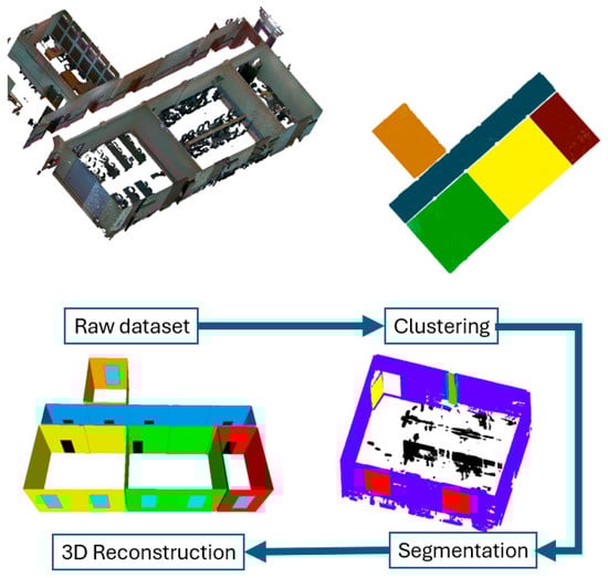
Figure 1.
Adopted flowchart for automatic 3D reconstruction from point cloud.
2.1. Clustering
The proposed approach begins by fragmenting the entire scene into smaller components, which are then processed individually. Preprocessing is conducted using two primary filtering techniques: voxel-based downsampling and statistical outlier removal. The latter is performed using the median and median absolute deviation (MAD) rather than the traditional mean and standard deviation, due to the improved robustness of MAD in identifying outliers [23]. To segment the scene into separate rooms, the DBSCAN [27] algorithm is applied to the point cloud projected onto the 2D (XY) plane. For indoor environments, a spacing threshold of 0.06 m—approximately half the average wall thickness (0.12 m)—is used to distinguish between clusters. The results of the clustering process for all rooms in the tested scene are illustrated in Figure 2.
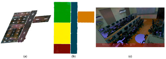
Figure 2.
Room clustering: (a) point cloud projection in XY plane and (b) cluster results using DBSCAN; (c) one cluster with furniture.
2.2. Segmentation
The segmentation process aims to extract object classes present within each clustered room. It consists of two main steps: density map analysis and deep learning-based segmentation using the RandLA-Net model.
The focus is placed on identifying structural components of the building, including walls, floors, ceilings, and wall-surface features such as doors and windows. Since wall elements generally exhibit the highest elevation, their projection onto the XY plane results in regions with elevated point density. To quantify this density, a predefined radius is assigned to each point, within which neighboring points are counted. An 8 cm threshold—chosen to be smaller than the minimum typical wall thickness—is used to define the search radius for density estimation.
For the automated extraction of high-density regions, an arithmetic mean is calculated across all point densities, and only points exceeding this mean are retained. The resulting density distribution is illustrated by a histogram in Figure 3a. However, despite the effectiveness of this method in identifying structural regions, cluttered areas are often preserved, demonstrating that density analysis alone is insufficient for fully removing non-structural elements, as also shown in Figure 3b–d.
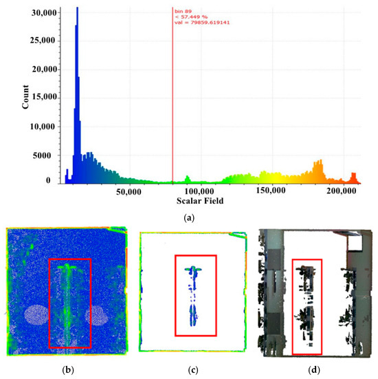
Figure 3.
Density analysis: (a) density histogram, (b) point density in XY plane, (c,d) results [blue for low density red for high density, and red box to highlight changes].
To address the challenge of high clutter, deep learning-based segmentation was performed using RandLA-Net. The model was trained on the Stanford Large-Scale 3D Indoor Spaces (S3DIS) dataset, which contains six indoor areas and 13 annotated semantic classes (ceiling, floor, wall, beam, column, window, door, chair, table, bookcase, sofa, board, and clutter). Following the official 6-fold protocol, five areas were used for training (see Figure 4), and one held-out area for testing (training was on Areas 1, 2, 3, 4 and testing on Area 5). This ensures that no points or scenes from the test area appear in the training or validation sets.
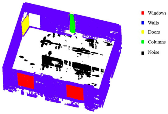
Figure 4.
Applying the RandLA-Net algorithm to a room cluster.
Each input block contained 4096 randomly sampled points normalized to local coordinates. Standard geometric augmentations were applied, including random rotation around the vertical axis, scaling, and jittering. Training was performed using the Adam optimizer with an initial learning rate of 0.01, decayed by 0.95 per epoch. The batch size was set to 8 for training and 16 for validation, and the network was trained for 100 epochs. A class-weighted cross-entropy loss was used to mitigate class imbalance. No pretraining or external data were used.
The results of applying the segmentation algorithm to the tested cluster are presented in Figure 5. As illustrated, the points within the room were segmented into five distinct classes. The majority of points were assigned to the wall class, while others were classified as columns, doors, and windows. The remaining points were labeled as noise. Notably, points associated with a room divider were categorized as noise, as the divider was only partially preserved during the preceding density filtering step and therefore did not conform to any of the trained object classes.
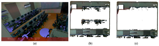
Figure 5.
Segmentation analysis for detection of structural elements: (a) raw cluster data, (b) initial results after applying density map analysis, and (c) RandLA-Net segmentation results.
2.3. Three-D Reconstruction
The reconstruction of 3D structural elements from the segmented results requires the extraction of planar primitives. These planar primitives are identified using the RANSAC algorithm, which is a robust model-fitting technique capable of handling datasets with significant noise or outliers—up to 50% of the points. RANSAC is particularly effective in detecting planes within point clouds, even when a substantial portion of the data is corrupted. Moreover, it is computationally efficient and widely supported across various programming platforms.
The general form of a plane equation derived from a point cloud is expressed as:
where = set of 3D points {, ,…., }, is normal vector = [, , ] and a distance from the origin
By applying RANSAC to the segmented dataset, planar primitives are extracted, as illustrated in Figure 6a. The RANSAC plane fitting was performed with a distance threshold of 0.5 m, 500 iterations, and three randomly sampled points (initₙ = 3) per model hypothesis. This threshold represents the maximum distance used to cluster nearby planar points during segmentation, rather than the inlier tolerance of the RANSAC plane model itself. The process iteratively detects dominant planes until less than 50% of the input points remain unassigned (min ratio = 0.5). A key advantage of RANSAC is that it provides the mathematical equations of the detected planes. These equations enable the computation of intersection points between primary planar surfaces, which are essential for generating the 2D floor plan. Examples of such intersection calculations are provided in Equations (3) and (4).

Figure 6.
Results of the RANSAC-based planar detection and modeling. (a) Detected planar primitives visualized in distinct colors. (b) Extracted intersection points corresponding to a selected cluster. (c) Initial mesh model generated from inlier points. (d) Refined mesh model after applying interpolation techniques.
To address occlusion or incomplete surfaces in the detected planes, interpolation is applied using the derived plane equations and the inlier points. A distance threshold of 10 cm between vertices is used to fill gaps and ensure surface continuity. Figure 6c,d visualize the differences between point clouds before and after interpolation.
The equations used for interpolation are as follows:
Openings within each wall are detected using a method adapted from the approach proposed by [23], with a projection threshold of 1.0 m applied to points located on the planar wall surface. Histogram analysis is then performed on each wall plane to identify boundary regions. This analysis distinguishes between two categories of points, namely, high-intensity points (those exceeding the average intensity) and low-density points (fewer than 50 points per 10 cm), which typically correspond to wall openings such as doors and windows. These two classes—representing the highest and lowest density regions—are then combined to delineate the wall boundaries, as illustrated in Figure 7a,b. The pseudocode provided in Appendix A summarizes the full workflow of the proposed method and reflects the default parameter settings used in all reported experiments.

Figure 7.
Wall border detection: (a) boundaries of high density, (b) histogram plot in the xy plane, (c) inliers and outlier boundaries, and (d) final reconstructed mesh model.
3. Evaluation
The performance of the proposed approach is assessed using three standard metrics, namely, completeness, correctness, and accuracy, as defined by [28,29]. These metrics are employed to evaluate the structural components of the generated model. A detailed explanation of each metric is provided in the following subsections.
3.1. Completeness
Completeness measures the extent to which the generated model captures the structure present in the reference model (). This is assessed by computing the overlap between the reference model and the generated model (), where the overlap is defined as the area of intersection between corresponding surfaces in the reference model and in the generated model.
The area of intersection is calculated by projecting each surface in the generated model onto the reference model and evaluating the overlap with each surface . The union of these overlapping regions is used to avoid double-counting. To enhance robustness, the completeness is calculated based on the total union area of all intersections, rather than summing individual overlap areas separately.
The completeness metric is formally expressed as:
where denotes the orthogonal projection of the generated surface onto the reference model.
3.2. Correctness
The metric of correctness is conceptually analogous to that of completeness, as it evaluates the extent to which the generated model aligns with the reference model. However, while completeness measures the proportion of the reference model captured by the generated model, correctness assesses the proportion of the generated model that intersects with the reference model. Specifically, this is achieved by modifying the completeness equation: the denominator, originally representing the surface area of the reference model, is replaced with the surface area of the generated model.
3.3. Accuracy
Accuracy is evaluated by measuring the geometric discrepancy between the generated model and the reference model. This is achieved by calculating the distances between individual sample points , which represent the reference model, and the nearest corresponding surfaces in the generated model. The error magnitude is quantified using the median absolute distance, as defined in Equation (7). To reduce the influence of outliers, a maximum distance threshold is imposed, beyond which any error values are capped.
4. Datasets
The proposed method was evaluated using a diverse set of indoor point cloud datasets, selected to capture a wide range of structural configurations and complexity levels. These datasets include both Manhattan and non-Manhattan layouts, simple and intricate geometries, and scenes with constant as well as variable ceiling heights. A summary of their specifications is presented in Table 2. The first dataset, acquired with a mobile laser scanner, depicts Manhattan-world geometry and features a long corridor with minimal clutter limited to decorative elements. The second dataset, referred to as the fire brigade scene, was captured in the office of fire brigade in Delft, The Netherlands, using Leica C10 terrestrial laser scanner. It also follows Manhattan geometry and comprises nine rooms and a large hall with a high density of clutter such as chairs and desks. The third dataset, also from UZH, represents a single non-Manhattan room heavily furnished with desks and bookshelves. The fourth dataset, an office scene, combines Manhattan and non-Manhattan spaces across multiple rooms, with significant clutter from office furniture. The fifth dataset, a cottage scene, maintains a Manhattan layout but incorporates varying ceiling heights and moderate clutter. The sixth dataset, Grainger Museum, represents a large non-Manhattan layout characterized by extensive clutter.
Table 2.
Dataset description.
In addition to these datasets, the evaluation included a point cloud collected at the Construction Engineering Technology Laboratory (CETL), Faculty of Engineering, Cairo University. This dataset was acquired using a BLK360 terrestrial laser scanner and follows a Manhattan-world configuration. It consists of five rooms connected by a long corridor, with substantial clutter from desks, chairs, and air conditioning units, providing a challenging scenario for structural element detection.
5. Discussion
This section presents a comprehensive evaluation of the proposed approach through four key stages. First, the sensitivity of the method to the predefined threshold parameters is examined. Second, an ablation study is conducted to assess the contribution of individual components within the processing pipeline. Third, the performance of the approach in detecting structural openings is evaluated. Finally, the overall effectiveness of the proposed method is analyzed across seven benchmark datasets. Each of these aspects is discussed in detail in the following subsections.
5.1. Sensitivity Study
Different parameter settings were adopted in the proposed pipeline (DBSCAN ε = 0.06 m; density radius = 0.08 m; opening projection = 1.0 m; and histogram low-count threshold = 50 points per 10 cm). A sensitivity analysis was then conducted to evaluate the robustness of these parameters. Each parameter was varied at three levels—0.5×, 1.0×, and 1.5× its default value—using a representative non-Manhattan scene (Office 2). The results are summarized in Table 3. The DBSCAN ε and histogram threshold exhibited the largest influence on reconstruction completeness, correctness, and geometric accuracy (up to ±15% variation), whereas the density radius and opening projection parameters showed minor sensitivity (±5–8%). Overall, the pipeline remained stable across a broad parameter range, confirming that the default values are appropriate for general indoor reconstruction tasks.
Table 3.
Sensitivity analysis of key geometric parameters in the reconstruction pipeline. Each parameter was varied by ±50% around its default value while others were kept fixed. The default configuration yields completeness = 97.6%, correctness = 98.2%, and mean geometric error = 2.4 cm.
These variations can be explained by the role each parameter plays in the reconstruction process. The DBSCAN ε parameter directly controls room partitioning, so smaller values tend to over-segment walls and lose completeness, while larger values merge adjacent spaces and reduce correctness. Similarly, the histogram threshold determines how small or noisy wall patches are filtered; if set too low, clutter is mistaken for structure, and if too high, valid thin walls are removed. In contrast, the density radius and opening projection affect only local smoothing and door/window estimation—processes that are less sensitive to moderate parameter shifts—resulting in more stable performance across their tested ranges.
5.2. Ablation Study of Pipeline Components
To assess the individual impact of each processing stage within the proposed hybrid pipeline, an ablation study was carried out using the indoor point cloud (CETL dataset). The analysis focused on three main modules:
- Density prefiltering before semantic segmentation (RandLA-Net).
- Semantic/density masking during planar fitting (RANSAC).
- Histogram-based refinement in wall-opening detection.
Each experiment was performed using the same RandLA-Net model weights, default parameters, and evaluation metrics—completeness, correctness, and geometric accuracy—were calculated (see Table 4). The full pipeline (density + DL + RANSAC + histogram refinement) serves as the baseline.
Table 4.
Ablation study on our dataset showing the effect of density filtering, semantic/density masking, and histogram refinement on indoor reconstruction accuracy.
The results on the CETL dataset confirm the importance of each pipeline module. Removing the density prefiltering stage reduces completeness by over 7% and correctness by 6–7%, demonstrating that eliminating outlier and background points prior to segmentation significantly improves the network’s learning of structural geometry. Introducing semantic and density masks during RANSAC fitting improves geometric consistency by preventing false planar fits on furniture and noise.
Finally, the histogram-based refinement step is essential for accurate opening detection—its absence increases false positives and misses slender door/window gaps. Together, these results validate that the hybrid combination of geometric filtering, semantic segmentation, and statistical refinement is crucial for achieving high-fidelity reconstructions.
5.3. Opening Detection Evaluation
To further verify the robustness of the evaluation metrics and the reliability of opening detection, additional analyses were conducted using the CETL dataset. The “accuracy = X cm @ 10 cm” values reported earlier in Table 3 correspond to the median point-to-surface distance computed with a maximum cap distance of 10 cm. This cap limits the influence of outliers and missing regions. This capped distance provides a stable geometric measure for comparing different datasets, but its interpretation depends on the chosen buffer size.
To confirm that the evaluation is not biased by this threshold, symmetric surface-distance metrics were also computed. These include the bidirectional Chamfer distance and the 95th-percentile Hausdorff distance, which evaluate surface proximity in both directions. The obtained values—2.6 cm (Chamfer) and 5.8 cm (95th-percentile Hausdorff)—indicate strong geometric agreement between the reconstructed and reference surfaces even without buffer dependence. Since accurate localization of wall openings (doors and windows) is one of the key contributions of this study, a precision–recall analysis was also conducted using manually annotated ground-truth openings from our dataset, within a 10 cm spatial tolerance. A prediction was considered correct if at least 70% of its projected area overlapped with a ground-truth opening. The results, summarized in Table 5, demonstrate that the proposed histogram-refinement step improves both precision and recall. It reduces false positives caused by clutter while recovering narrow openings missed by earlier steps.
Table 5.
Precision–recall evaluation of wall-opening detection on CETL dataset (10 cm tolerance).
5.4. Overall Effectiveness of the Proposed Method
To assess the effectiveness of the proposed approach for automatic reconstruction from unstructured point clouds, multiple datasets with varying characteristics were evaluated. The process of clustering unstructured point clouds into multiple rooms is demonstrated through the presented methodology. The proposed approach effectively handles complex indoor environments, including those with dense furniture arrangements. It performs well regardless of whether the layout adheres to Manhattan world assumptions (Figure 8a) or deviates from them (Figure 9). Initially, statistical outlier removal is performed using the median and MAD, followed by the application of the DBSCAN algorithm. A spatial threshold of 0.06 m—smaller than the typical wall thickness—was employed. This enables the successful identification of even narrow architectural features such as doorways and corridors (Figure 8b).

Figure 8.
Cottage dataset: (a) raw point cloud and (b) clustering result.

Figure 9.
Grainger Museum dataset: (a) raw point cloud and (b) clustering result.
Each cluster identified within the scene is processed using the proposed hybrid segmentation strategy, which integrates density map analysis with deep learning-based segmentation employing the RandLA-Net model. This combined approach effectively detects most pieces of furniture and clutter. It also enables accurate identification of planar surfaces such as walls, ceilings, and floors. During the density analysis phase, specific features of the datasets become apparent. For example, in the fire brigade dataset, glass partitions framed in wood within the hall produce high-density regions when projected onto a 2D plane (Figure 10a). Similarly, the shower enclosures in the bathrooms of the cottage dataset generate comparable high-density zones upon projection (Figure 10b). When the RandLA-Net deep learning model is applied to these high-density regions, it accurately segments non-structural elements—such as bookshelves, paper storage units, and shower enclosures—into either the bookshelf class or categorizes them as noise if they do not match any predefined classes within the model. The segmentation results for the evaluated datasets are illustrated in Figure 11 and Figure 12. In the hallway dataset, most of the point cloud was segmented as walls. Notably, the proposed method successfully detected and reconstructed indoor scenes with complex architectural features, including slanted ceilings as shown in Figure 8 and Figure 11.

Figure 10.
Density analysis results: (a) fire brigade dataset; (b) cottage dataset.
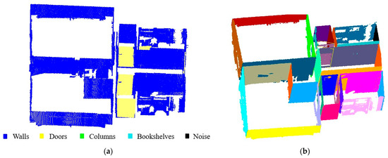
Figure 11.
Results of (a) segmentation and (b) planar surface detection for cottage dataset.
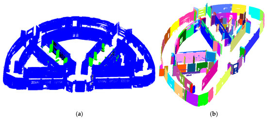
Figure 12.
Results of (a) segmentation results and (b) planar surface detection for Grainger Museum dataset.
The 3D reconstruction process involves the detection of planar primitives, wall surface object detection, and subsequent reconstruction of 2D floor plans and 3D models. Planar primitives—as shown in Figure 11b and Figure 12b—are detected for each separate room and then integrated to enhance visual representation. It is important to highlight that a single wall may be detected as multiple planar segments, particularly in cases where structural elements such as columns interrupt the wall’s continuity. However, these numerous detected planes will not affect the result negatively. They only increase the processing time slightly as each plane is processed and interpolated separately.
The reconstruction of 2D floor plans and 3D models is based on extracting the corners of each room and the corners of the wall surface openings. It should be noted that in the generation of 2D floor plans (Figure 13a and Figure 14a), each room is drawn and finished, and then the algorithm moves to the next room, which gives our approach the advantage of showing the thickness in the layout. It should also be noted that doors and windows are modeled as closed plans no matter if they were opened or closed during data acquisition. This will not affect the quality of the final model as our purpose is to locate the wall surface openings and their dimensions. The final 3D reconstruction results are presented in Figure 13b and Figure 14b.

Figure 13.
Office 2 dataset final reconstruction results: (a) 2D floor plan for AutoCAD (2023) and (b) 3D reconstructed model.

Figure 14.
Cottage dataset final reconstruction results: (a) 2D floor plan for AutoCAD and (b) 3D reconstructed model. (D for door, W for window).
While histogram analysis was performed on each wall plane to identify boundary regions for wall surface openings and the histogram-based refinement approach effectively enhances opening detection by filtering low-density regions along wall planes, several scene-dependent challenges remain. Table 6 summarizes per-scene detection results for all seven representative indoor datasets used in this study, illustrating that the method performs consistently across various layouts but degrades slightly in scenes with extensive transparent or reflective surfaces.
Table 6.
Per-scene precision and recall for door and window detection.
Most errors occur in scenes containing glass partitions, reflective displays, or recessed openings, where point density along wall planes does not clearly distinguish between solid and open regions. In such cases, transparent elements and bookcases can appear as high-density “false walls”, masking true openings.
For evaluation of the whole scene for each dataset, reference floor plans were manually delineated in 2D space and compared with the corresponding outputs generated by the algorithm. Table 7 presents an overview of the datasets used for testing, along with their associated performance metrics.
Table 7.
Evaluation results for tested datasets @ 10 cm buffer distance.
The cottage dataset, which features slanted ceilings, achieved the highest accuracy—1.3 cm—within a 10 cm buffer. In contrast, the fire brigade dataset exhibited the lowest accuracy at 9.6 cm, which can be attributed to the high level of clutter and inconsistencies in the point cloud data acquired from that environment.
In terms of completeness and correctness, the proposed approach consistently delivered high value across datasets. The results demonstrate that the method is robust and generalizable across a variety of indoor settings, including those with Manhattan and non-Manhattan layouts, different levels of clutter, and variable ceiling heights.
Table 8 presents a comparison between the previous work [30], evaluated on the fire brigade dataset, and the proposed approach. A comparison between Table 7 and Table 8 highlights that the proposed approach achieves higher completeness and correctness scores than prior benchmarks, confirming its improved reliability in reconstructing complex and cluttered indoor environments.
Table 8.
Fire brigade results from different approaches.
The computational efficiency of the proposed hybrid reconstruction pipeline was evaluated based on consumed runtime and memory consumption (see Table 9); they were measured on a workstation equipped with an Intel® Core™ i7-10750 CPU @ 2.60 GHz, 32 GB RAM, and an NVIDIA® GTX 1060 Ti GPU (6 GB VRAM).
Table 9.
Per-scene runtimes and peak memory.
In terms of computational complexity, the overall pipeline scales approximately as with respect to the number of input points . DBSCAN and local density computation dominate the preprocessing stage, each operating near , while RandLA-Net inference and RANSAC plane fitting scale linearly with the number of processed points. This ensures good scalability for large indoor scans, consistent with the runtime results reported in Table 9.
6. Conclusions
An automated approach for the reconstruction and modeling of three-dimensional indoor geometrical structures from unstructured point clouds has been presented. The process begins with room clustering using the DBSCAN algorithm to partition the scene. Density map analysis is then applied to the 2D-projected point cloud to retain only high-density points, effectively filtering out non-structural elements.
Point cloud segmentation is performed using the deep learning-based RandLA-Net model. Following segmentation, planar surface extraction is carried out using the RANSAC algorithm. Wall boundaries and openings are defined through density-based calculations, and wall-surface openings are refined by identifying inliers and outliers. Points obstructing wall openings are treated as outliers and removed through interpolation techniques. The process concludes with the generation of mesh models, planimetric models, and 2D floor plans for the entire scene.
The proposed method was evaluated across various indoor environments, including those with Manhattan and non-Manhattan geometries, as well as slanted and non-slanted ceilings. The evaluation was based on three standard metrics: completeness, correctness, and accuracy. The results demonstrated a minimum of 86.6% completeness, 84.8% correctness, and up to 1.3 cm accuracy, confirming the robustness and generalizability of the proposed approach across diverse indoor scenarios.
Author Contributions
Conceptualization, Youssef Hany and Wael Ahmed; methodology, Youssef Hany and Wael Ahmed; software, Youssef Hany; validation, Wael Ahmed, Walid Darwish and Ahmad M. Senousi; formal analysis, Youssef Hany, Wael Ahmed and Walid Darwish; investigation, Walid Darwish and Ahmad M. Senousi; writing—original draft preparation, Youssef Hany and Wael Ahmed; writing—review and editing, Wael Ahmed and Walid Darwish; visualization, Youssef Hany; supervision, Wael Ahmed and Adel Elshazly; project administration, Adel Elshazly. All authors have read and agreed to the published version of the manuscript.
Funding
This research received no external funding.
Data Availability Statement
The datasets used in this study will be made available upon request.
Acknowledgments
We acknowledge the Visualization and Multimedia Lab at the University of Zurich (UZH) and Claudio Mura for the acquisition of the 3D point clouds, and UZH as well as ETH Zürich for their support in scanning the rooms represented in these datasets. We would also like to acknowledge the Construction Engineering Technology Lab (CETL)—Faculty of Engineering, Cairo University, for their support of the laser scanner dataset which we used for testing each step in our proposed method.
Conflicts of Interest
Authors Ahmad M. Senousi and Walid Darwish are currently employed by Namaa for Engineering Consultations on part-time basis also was employed by Cairo University on full time basis. The remaining authors declare that the research was conducted in the absence of any commercial or financial relationships that could be construed as a potential conflict of interest.
Appendix A. Pseudocode of the Proposed 3D Reconstruction Pipeline
1. Preprocessing
1.1 P_down ← VOXEL_DOWNSAMPLE(P, voxel_size)
1.2 P_clean ← STATISTICAL_OUTLIER_REMOVAL(P_down)//use median + MAD
1.3 Normalize coordinates if needed (coordinate system)
2. Room partitioning
2.1 P_xy ← PROJECT_TO_XY(P_clean)
2.2 clusters ← DBSCAN(P_xy, eps = dbscan_eps, minpts = dbscan_minpts)
2.3 For each cluster c in clusters:
create partition Pc = points in P_clean with cluster id = c
3. For each partition Pc do
3.1 Density prefiltering (optional/adaptive)
//compute local density per point
For each p in Pc:
n_p ← COUNT_POINTS_WITHIN_RADIUS(Pc, p, density_radius)
//keep only points with n_p > avg_density OR use adaptive percentile
wall_candidates ← { p in Pc | n_p >= THRESH_DENSITY }
//note: ablation (RandLA-Net only): skip this step and set wall_candidates = Pc
3.2 Semantic segmentation (RandLA-Net inference)
//input: blocks sampled from wall_candidates (or Pc if prefilter skipped)
labels ← RANDLANET_INFERENCE(wall_candidates, block_points = randlanet_block_points)
//produce boolean masks:
mask_structural ← labels in {wall, floor, ceiling, column}
mask_opening_candidates ← labels in {door, window}
3.3 Combine density + semantic masks
//final mask for plane fitting
fit_points ← wall_candidates ∩ mask_structural
//for ablation: try fit_points_alt = mask_structural (no density mask)
3.4 RANSAC plane detection and fitting
planes ← []
remaining_points ← fit_points
while size(remaining_points) > min_inliers:
plane, inliers ← RANSAC_FIT_PLANE(remaining_points, threshold = t_plane)
if |inliers| < MIN_INLIERS: break
planes.append(plane, inliers)
remaining_points ← remaining_points\inliers
//optionally merge collinear/coplanar planes
planes ← MERGE_SIMILAR_PLANES(planes, angular_tol, dist_tol)
3.5 Plane interpolation/gap-filling
For each plane in planes:
boundary ← PROJECT_INLIERS_TO_PLANE(plane.inliers)
//fill small gaps using interpolation (max_gap = 0.10 m)
polygon ← INTERPOLATE_BOUNDARY(boundary, max_edge_len = 0.10)
add polygon to model M (as wall/ceiling patch)
3.6 Opening detection (histogram refinement)
For each wall_plane in planes labelled as wall:
//define wall-aligned 2D coordinate frame (u,v) on plane
W_points ← points projected to wall_plane
//build 2D histogram on wall plane (cell size e.g., 0.1 m)
hist ← BUILD_2D_HISTOGRAM(W_points, cell_size = 0.10)
//identify low-density cells
low_cells ← {cell | hist[cell] < hist_thresh} //or percentile-based
//optionally combine with semantic opening mask
candidate_regions ← CONNECTED_COMPONENTS(low_cells)
//refine candidates (filter by area, shape, height)
For each region r in candidate_regions:
if AREA(r) < MIN_OPENING_AREA: continue
if HEIGHT_PROFILE_VALID(r, W_points): accept
else reject
Record accepted openings in O (with polygon and bounding box)
4. Post-processing & model assembly
4.1 Merge planar patches across partitions (align walls across cluster borders)
4.2 Snap intersections → compute 2D floorplan corners
4.3 Attach openings O to corresponding wall polygons
5. Evaluation & Reporting
5.1 Compute completeness, correctness using projection-based overlap metrics
5.2 Compute accuracy as median (min (distances, d_cap))
5.3 Compute symmetric metrics (Chamfer, Hausdorff_95) for robustness
Return M, O
End Procedure
References
- Thomson, C.; Boehm, J. Automatic Geometry Generation from Point Clouds for BIM. Remote Sens. 2015, 7, 11753–11775. [Google Scholar] [CrossRef]
- Rocha, G.; Mateus, L.; Ferreira, V. Historical Heritage Maintenance via Scan-to-BIM Approaches: A Case Study of the Lisbon Agricultural Exhibition Pavilion. ISPRS Int. J. Geo-Inf. 2024, 13, 54. [Google Scholar] [CrossRef]
- Běloch, L.; Pavelka, K. Optimizing Mobile Laser Scanning Accuracy for Urban Applications: A Comparison by Strategy of Different Measured Ground Points. Appl. Sci. 2024, 14, 3387. [Google Scholar] [CrossRef]
- Wei, P.; Fu, K.; Villacres, J.; Ke, T.; Krachenfels, K.; Stofer, C.R.; Bayati, N.; Gao, Q.; Zhang, B.; Vanacker, E.; et al. A Compact Handheld Sensor Package with Sensor Fusion for Comprehensive and Robust 3D Mapping. Sensors 2024, 24, 2494. [Google Scholar] [CrossRef]
- Mahmoud, M.; Zhao, Z.; Chen, W.; Adham, M.; Li, Y. Automated Scan-to-BIM: A deep learning-based framework for indoor environments with complex furniture elements. J. Build. Eng. 2025, 106, 112596. [Google Scholar] [CrossRef]
- Xiang, Z.; Rashidi, A.; Ou, G. Integrating Inverse Photogrammetry and a Deep Learning–Based Point Cloud Segmentation Approach for Automated Generation of BIM Models. J. Constr. Eng. Manag. 2023, 149, 04023074. [Google Scholar] [CrossRef]
- Gan, V.J.L.; Hu, D.; Wang, Y.; Zhai, R. Automated indoor 3D scene reconstruction with decoupled mapping using quadruped robot and LiDAR sensor. Comput.-Aided Civ. Infrastruct. Eng. 2025, 40, 2209–2226. [Google Scholar] [CrossRef]
- Okorn, B.; Xiong, X.; Akinci, B.; Huber, D. Toward Automated Modeling of Floor Plans. In Proceedings of the Symposium on 3D Data Processing, Visualization and Transmission, Paris, France, 17–20 May 2010. [Google Scholar]
- Ambrus, R.; Claici, S.; Wendt, A. Automatic Room Segmentation from Unstructured 3-D Data of Indoor Environments. IEEE Robot. Autom. Lett. 2017, 2, 749–756. [Google Scholar] [CrossRef]
- Jung, J.; Stachniss, C.; Kim, C. Automatic Room Segmentation of 3D Laser Data Using Morphological Processing. ISPRS Int. J. Geo-Inf. 2017, 6, 206. [Google Scholar] [CrossRef]
- Pouraghdam, M.H.; Saadatseresht, M.; Rastiveis, H.; Abzal, A.; Hasanlou, M. Building Floor Plan Reconstruction from SLAM-Based Point Cloud using RANSAC Algorithm. Int. Arch. Photogramm. Remote Sens. Spat. Inf. Sci. 2019, XLII-4/W18, 483–488. [Google Scholar] [CrossRef]
- Zhang, Y.; Luo, C.; Liu, J. Walk&sketch: Create floor plans with an RGB-D camera. In Proceedings of the 2012 ACM Conference on Ubiquitous Computing, New York, NY, USA, 5–8 September 2012; pp. 461–470. [Google Scholar] [CrossRef]
- Previtali, M.; Barazzetti, L.; Brumana, R.; Scaioni, M. Towards automatic indoor reconstruction of cluttered building rooms from point clouds. ISPRS Ann. Photogramm. Remote Sens. Spat. Inf. Sci. 2014, II-5, 281–288. [Google Scholar] [CrossRef]
- Díaz-Vilariño, L.; Khoshelham, K.; Martínez-Sánchez, J.; Arias, P. 3D Modeling of Building Indoor Spaces and Closed Doors from Imagery and Point Clouds. Sensors 2015, 15, 3491–3512. [Google Scholar] [CrossRef] [PubMed]
- Sanchez, V.; Zakhor, A. Planar 3D modeling of building interiors from point cloud data. In Proceedings of the 2012 19th IEEE International Conference on Image Processing, Orlando, FL, USA, 30 September–3 October 2012; pp. 1777–1780. [Google Scholar] [CrossRef]
- Oesau, S.; Lafarge, F.; Alliez, P. Indoor scene reconstruction using feature sensitive primitive extraction and graph-cut. ISPRS J. Photogramm. Remote Sens. 2014, 90, 68–82. [Google Scholar] [CrossRef]
- Xiao, J.; Furukawa, Y. Reconstructing the World’s Museums. Int. J. Comput. Vis. 2014, 110, 243–258. [Google Scholar] [CrossRef]
- Prieto, S.A.; Quintana, B.; Adán, A.; Vázquez, A.S. As-is building-structure reconstruction from a probabilistic next best scan approach. Rob. Auton. Syst. 2017, 94, 186–207. [Google Scholar] [CrossRef]
- Zavar, H.; Arefi, H.; Malihi, S.; Maboudi, M. Topology-Aware 3D Modelling of Indoor Spaces from Point Clouds. Int. Arch. Photogramm. Remote Sens. Spat. Inf. Sci. 2021, XLIII-B4-2, 267–274. [Google Scholar] [CrossRef]
- Mura, C.; Mattausch, O.; Pajarola, R. Piecewise-planar Reconstruction of Multi-room Interiors with Arbitrary Wall Arrangements. Comput. Graph. Forum 2016, 35, 179–188. [Google Scholar] [CrossRef]
- Ochmann, S.; Vock, R.; Wessel, R.; Klein, R. Automatic reconstruction of parametric building models from indoor point clouds. Comput. Graph. 2016, 54, 94–103. [Google Scholar] [CrossRef]
- Murali, S.; Speciale, P.; Oswald, M.R.; Pollefeys, M. Indoor Scan2BIM: Building information models of house interiors. In Proceedings of the 2017 IEEE/RSJ International Conference on Intelligent Robots and Systems (IROS), Vancouver, BC, Canada, 24–28 September 2017; pp. 6126–6133. [Google Scholar] [CrossRef]
- Shi, W.; Ahmed, W.; Li, N.; Fan, W.; Xiang, H.; Wang, M. Semantic Geometric Modelling of Unstructured Indoor Point Cloud. ISPRS Int. J. Geo-Inf. 2018, 8, 9. [Google Scholar] [CrossRef]
- Ochmann, S.; Vock, R.; Klein, R. Automatic reconstruction of fully volumetric 3D building models from oriented point clouds. ISPRS J. Photogramm. Remote Sens. 2019, 151, 251–262. [Google Scholar] [CrossRef]
- Biljecki, F.; Ledoux, H.; Stoter, J.; Zhao, J. Formalisation of the level of detail in 3D city modelling. Comput. Environ. Urban Syst. 2014, 48, 1–15. [Google Scholar] [CrossRef]
- Sánchez-Aparicio, L.J.; Castro, Á.B.-D.; Conde, B.; Carrasco, P.; Ramos, L.F. Non-destructive means and methods for structural diagnosis of masonry arch bridges. Autom. Constr. 2019, 104, 360–382. [Google Scholar] [CrossRef]
- Deng, D. DBSCAN Clustering Algorithm Based on Density. In Proceedings of the 2020 7th International Forum on Electrical Engineering and Automation (IFEEA), Hefei, China, 25–27 September 2020; pp. 949–953. [Google Scholar] [CrossRef]
- Tran, H.; Khoshelham, K.; Kealy, A. Geometric comparison and quality evaluation of 3D models of indoor environments. ISPRS J. Photogramm. Remote Sens. 2019, 149, 29–39. [Google Scholar] [CrossRef]
- Senousi, A.M.; Ahmed, W.; Liu, X.; Darwish, W. Automated Digitization Approach for Road Intersections Mapping: Leveraging Azimuth and Curve Detection from Geo-Spatial Data. ISPRS Int. J. Geo-Inf. 2025, 14, 264. [Google Scholar] [CrossRef]
- Khoshelham, K.; Tran, H.; Acharya, D.; Vilariño, L.D.; Kang, Z.; Dalyot, S. The ISPRS Benchmark on Indoor Modelling-Preliminary Results. Int. Arch. Photogramm. Remote Sens. Spat. Inf. Sci. 2020, XLIII-B5-2, 207–211. [Google Scholar] [CrossRef]
- Maset, E.; Magri, L.; Fusiello, A. Improving Automatic Reconstruction of Interior Walls from Point Cloud Data. Int. Arch. Photogramm. Remote Sens. Spat. Inf. Sci. 2019, XLII-2/W13, 849–855. [Google Scholar] [CrossRef][Green Version]
- Tran, H.; Khoshelham, K. A Stochastic Approach to Automated Reconstruction of 3D Models of Interior Spaces from Point Clouds. ISPRS Ann. Photogramm. Remote Sens. Spat. Inf. Sci. 2019, IV-2/W5, 299–306. [Google Scholar] [CrossRef][Green Version]


Disclaimer/Publisher’s Note: The statements, opinions and data contained in all publications are solely those of the individual author(s) and contributor(s) and not of MDPI and/or the editor(s). MDPI and/or the editor(s) disclaim responsibility for any injury to people or property resulting from any ideas, methods, instructions or products referred to in the content. |
© 2025 by the authors. Published by MDPI on behalf of the International Society for Photogrammetry and Remote Sensing. Licensee MDPI, Basel, Switzerland. This article is an open access article distributed under the terms and conditions of the Creative Commons Attribution (CC BY) license (https://creativecommons.org/licenses/by/4.0/).