Landslide Susceptibility Assessment in the Japanese Archipelago Based on a Landslide Distribution Map

Abstract

Though danger prediction and countermeasures for landslides are important, it is fundamentally difficult to take preventive measures in all areas susceptible to dangerous landslides. Therefore, it is necessary to perform landslide susceptibility mapping, extract slopes with high landslide hazard/risk, and prioritize locations for conducting investigations and countermeasures. In this study, landslide susceptibility mapping along the whole slope of the Japanese archipelago was performed using the analytical hierarchy process (AHP) method, and geographic information system analysis was conducted to extract the slope that had the same level of hazard/risk as areas where landslides occurred in the past, based on the ancient landslide topography in the Japanese archipelago. The evaluation factors used were elevation, slope angle, slope type, flow accumulation, geology, and vegetation. The landslide susceptibility of the slope was evaluated using the score accumulation from the AHP method for these evaluation factors. Based on the landslide susceptibility level (I to V), a landslide susceptibility map was prepared, and landslide susceptibility assessment in the Japanese archipelago was identified. The obtained landslide susceptibility map showed good correspondence with the landslide distribution, and correlated well with past landslide occurrences. This suggests that our method can be applied to the extraction of unstable slopes, and is effective for prioritizing and implementing preventative measures.

1. Introduction

The Japanese archipelago is located near a converging plate boundary, and sediment disasters related to earthquakes and volcanoes, typhoons, and heavy rainfall occur frequently, reflecting topographical, geological, and meteorological conditions; thus, it is known as the global leader in sediment disasters. In particular, the geomorphology and geology of the Japanese archipelago are widely distributed in fragile ground and steep landforms because there are many products of magmatic activity, crustal deformation, and weathering, as well as hydrothermal alteration, fractured, and weathered zones that are widely distributed throughout the strata. Therefore, many sediment-related disasters have occurred due to landslides and slope failures that were triggered by rainfall and earthquakes. In the Japanese archipelago, there are approximately 530,000 sediment-related disaster risk areas and 350,000 sediment-related disaster-warning zones (of which approximately 200,000 are sediment-related disaster special warning zones) [1]. There are many extreme areas/zones. According to the database of landslide distribution maps [2] published by the National Research Institute for Earth Science and Disaster Resilience (NIED), landslide topography has been confirmed at approximately 370,000 locations (Figure 1). Therefore, the danger prediction and countermeasures for landslides are crucial; however, it is fundamentally difficult to take preventive measures for all landslide hazardous locations. Therefore, it is necessary to perform landslide susceptibility mapping, extract slopes with high landslide hazard/risk, and to conduct investigations and countermeasures after regions are prioritized. Considering that new landslides often occur in ancient landslide areas, the landslide distribution map [2] remains valid data.

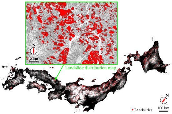
Figure 1. Landslide distribution map in the Japanese archipelago based on the NIED [2].

Naturally, although the Japanese archipelago varies in topography, geology, meteorological conditions, etc., for each region, it is important to effectively utilize the landslide topographic database and conduct landslide susceptibility assessments throughout the archipelago. However, very few cases of landslide susceptibility assessments throughout the Japanese archipelago have been reported. Therefore, this study attempted landslide susceptibility mapping using the AHP method and GIS analysis, and determined the landslide susceptibility of the entire Japan archipelago to extract slopes with the same hazard/risk as the areas with past landslide occurrences, based on landslide topography of the Japanese archipelago (Figure 1).

This study first conducted a literature review on landslide susceptibility mapping using the AHP method and GIS analysis. Secondly, we described the relationship between the landslide topography and evaluation factors/elements based on the landslide distribution map [2] in the target area. Thirdly, the procedure of setting the evaluation factors and method in landslide susceptibility assessment was briefly explained. Finally, landslide susceptibility mapping was performed, and the validity of the obtained maps was verified.

2. Literature Review

Presently, there have been many study cases in which the relationship between landslide topography and geology/landforms was examined using landslide distribution maps [2]. Particularly, Fujiwara et al. [3] clarified the geological divisions and topographical characteristics that define the landslide topographical distribution, using the landslide distribution map in the Japanese archipelago. Araiba et al. [4] clarified the relationship between the landslide distribution and geological characteristics based on the Japan landslide designated site survey report. In contrast, there have been many excellent studies on landslide hazard evaluation targeting each region globally. For example, Maeda et al. [5] summarized how to create a hydrothermal alteration zone landslide hazard map by scoring the landslide hazard in the Kanehana landslide area in Rubeshibe, northeastern Hokkaido, Japan, using the topography, geology, geological structure, and hydrothermal alteration zone of the whole slope, using the weighted slope allocation point method. Moriwaki and Sasaki [6] proposed a relative risk assessment method using the safety factor determined by dynamic slope stability analysis, assuming the circular landslide slope as an index, and prepared a hazard assessment map that was color coded into four levels according to the degree of safety in the Hachimantai area, Iwate, northern Japan. Lee et al. [7] performed landslide hazard mapping in Selangor, Malaysia, using landslide occurrence factors based on frequency ratio and logistic regression models. They listed landslide occurrence factors to be slope, aspect, curvature, distance from drainage, lithology, distance from lineaments, land cover, vegetation index, and precipitation distribution. Jiménez-Perálvarez et al. [8] used various methods (news reports, differential interferometric synthetic aperture radar, digital photogrammetry, light detection and ranging, photointerpretation, and dendrochronology) to perform landslide hazard mapping in the Betic Cordillera region in southern Spain. Bera et al. [9] performed landslide hazard mapping using a multi-criteria analysis method for the Eastern Himalayas, Namchi, South Sikkim. Then, based on the obtained landslide hazard map, the verification was conducted by field survey and geospatial technology-based analysis. Xu et al. [10] attempted to create a landslide risk assessment-zoning map based on landslide hazard and vulnerability assessment models, targeting landslide disasters in Xianyang City, Shaanxi Province. Batar et al. [11] evaluated the landslide susceptibility map by assigning weights to each class of 14 factors that cause landslides, using the weights of evidence (WoE) method, in the Indian Himalayan Region.

In recent years, a landslide hazard/risk assessment using geographic information systems (GIS) has been attempted, e.g., [12,13,14,15,16,17,18,19,20,21]. When limited to Japan, for example, Nagata et al. [12] analyzed the relationship between the distribution of unstable landslide topography, such as linear concave landslides, and topography/geology using GIS, for the range of 1/200,000 “Gifu” map width. Thus, a geological unit was identified where landslide topography may easily develop. Zhou et al. [13] proposed a novel preparation method of slope failure hazard mapping using GIS and quantification theory, applied it to the collapse case of Minamata City district in Kumamoto, Japan, and clarified that the proposed method is highly effective for preparing a precise hazard map. Hamasaki et al. [15] developed and proposed a buffer movement analysis and an error probability analysis method as a new analytical technique to complement various problems in slope change prediction evaluation, based on GIS, and applied it to landslides and slope failure cases caused by the Iwate-Miyagi Nairiku Earthquake in 2008. A case study of slope change prediction was evaluated using these techniques. However, several of these research results occurred because the objects of evaluation are limited within landslide landforms; this method was based on the consideration of reactive landslides, and subjective and empirical judgements of evaluators were strongly affected.

Several studies have been reported on the assessment of landslide risk using the analytic hierarchy process (AHP) method, e.g., [22,23,24,25,26,27,28,29,30,31,32,33,34]; thus, these subjective and empirical decisions can be evaluated as objectively as possible. The AHP method was first applied to judge the landslide topography risk, and Miyagi et al. [22] summarized the analysis technique. Since then, studies on landslide hazard assessment using the AHP method have been performed extensively, and applications of the method of Miyagi et al. [22] to various regions have been attempted. For example, Yagi et al. [24] developed a system for evaluating the risk of re-activity of landslide landforms using the AHP method, and applied it to 312 landslide slopes extracted in the Agano River middle basin (Fukushima and Niigata Prefectures) to create a re-activity risk distribution map of landslide topography. This evaluation system expresses the qualitative evaluation process by conventional aerial photograph interpretation, and can be utilized for quickly evaluating landslide hazards in a wide area without conducting a detailed field survey. Kohno and Maeda [26] attempted a landslide hazard assessment based on the AHP method, considering the mechanical properties of hydrothermally altered rocks based on the indefinite point load strength test, which could simply and quickly evaluate the rock strength, in addition to the topography, geology, geological structure, and hydrothermal alteration zones of the entire slope in the Ohekisawa-Shikerebenbetsugawa landslide area, Japan. Furthermore, the Geological Survey of Hokkaido [27] proposed a landslide hazard assessment technique that introduced the AHP method in Hokkaido district. However, many of these cases have been established through the brainstorming of several skilled engineers who have been conducting landslide surveys for many years, and there is a problem with the technique’s practical use as it requires sophisticated technology and time, and is largely based on the subjective and empirical judgment of the evaluators in terms of the way the evaluation items are subdivided.

3. Data and Materials

Though many landslide factors were considered in this study, the evaluation factors were set as “elevation”, “slope angle”, “slope type”, “flow accumulation”, “geology”, and “vegetation”.

The GIS software used was ArcGIS Pro by ESRI. GIS data models included vector, raster, and three-dimensional (3D) GIS data. The vector data were represented by three elements: points (points), lines (lines), and polygons (plane). The raster data comprised cells (pixels) arranged in a grid of rows and columns. The 3D GIS data had geographical 3D coordinate values: the X-axis and Y-axis plus the Z-axis (height). In this study, the landslide susceptibility scores for each evaluation factor calculated by the AHP method were input into each cell, and the raster data were applied (overlay) (Figure 2). The cell size of raster data was set at 20 m × 20 m.

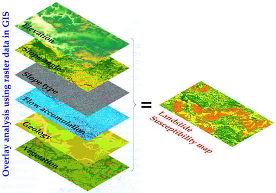
Figure 2. Overlay of the GIS model raster data.

3.1. Landslide Distribution Map Data

The landslide distribution map was generated by downloading the GIS data of the landslide distribution map [2] from the NIED. This map was a drawing in which 1:40,000 monochrome aerial photographs taken in the 1970s were interpreted by topographic interpretation using a simplified actual condition mirror of four magnifications, and its outline and basic structure (scarp and moving body) were mapped regarding “landslide topography”, which is a topographical trace formed by landslide fluctuation, and its distribution was shown in a 1:50,000 topographic map. This drawing extracted only relatively large landslide topography with a width of 150 m or more. Therefore, very small slope fluctuations, such as surface collapse, debris flow and falling rock, and landslide topography of 150 m or less in width, were not subject to interpretation, and no field survey was conducted on the interpreted topography. Therefore, the absence of a landslide topography on a map does not mean that there is no landslide topography [2]. As the scale of landslide topographies at approximately 370,000 locations confirmed in the Japanese archipelago varies in size, this study did not treat landslide topography (vector data) as point data (one cell of 20 m × 20 m). Instead, it expressed moving body parts (polygon data) of landslide topographies with raster data to create landslide topographies. Incidentally, the scarp (line data) was not subject to analysis because it did not have area information.

3.2. Topographic Data

Topographic data were downloaded from the basic map information (10 m mesh, Digital Elevation Model: DEM10B) [35] published by the Geographical Survey Institute (GSI). The number of download files totaled 4898, which covered the Japanese archipelago. Hereafter, “elevation”, “slope angle”, “slope type”, and “flow accumulation” of the Japanese archipelago, prepared by GIS software based on the DEM10B [35], are briefly described.

3.2.1. Elevation

Using the basement map information viewer converter, the DEM data were converted into an ArcGIS Pro format and expressed as a color-specific elevation diagram, as shown in Figure 3.

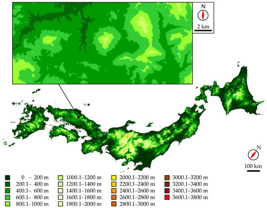
Figure 3. Elevation map of the Japanese archipelago.

As the highest peak in the Japanese archipelago is 3776.12 m at Mt. Fuji, located in the central part of the Japanese archipelago, elevations reaching 3800 m were divided into 200 m intervals (Figure 3). Approximately 70% of the Japanese archipelago comprises mountains and hills, and the spine mountains run in the central part. Areas above 500 m elevation and those below 100 m each account for approximately 25% of the region.

3.2.2. Slope Angle

Using the prepared “elevation” raster data, the slope angle was determined for all cells. The slope angle was calculated according to the maximum rate of change, comparing the altitude of the target cell and the neighboring cell. To perform the calculation, first we considered a plane (3d × 3d) whose side size is d [m] centered on the target cell z₅ (z represents the altitude), as shown in Figure 4.

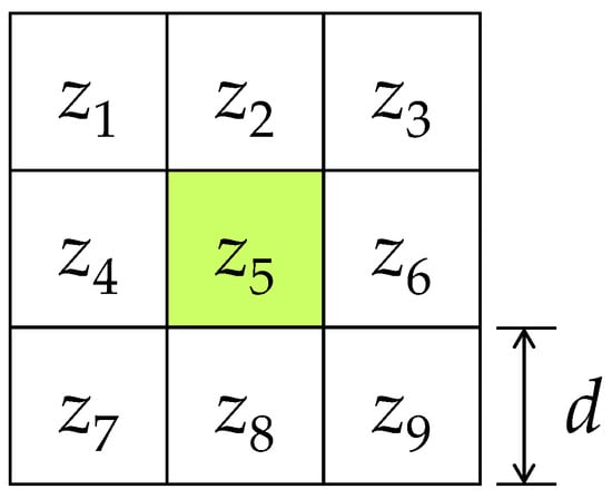
Figure 4. Cell model for GIS surface analysis.

Then, the rate of change in the x-direction and the y-direction of the central target cell was calculated by Equations (1) and (2), respectively.

$$\frac{dz}{dx}=\frac{\left(z_3+2z_6+z_9\right)-\left(z_1+2z_4+z_7\right)}{8d}$$

(1)

$$\frac{dz}{dy}=\frac{\left(z_7+2z_8+z_9\right)-\left(z_1+2z_2+z_3\right)}{8d}$$

(2)

Using the rate of change obtained by Equations (1) and (2), slope angle a was determined by the following equation:

$$a=\sqrt{{\left(\frac{dz}{dx}\right)}^2+{\left(\frac{dz}{dy}\right)}^2}$$

(3)

The above parameter can be easily obtained by executing the surface analysis of ArcGIS Pro, and the result is shown in Figure 5. In this study, the slope angle was divided into intervals of 10° (Figure 2). Most of the Japanese archipelago slope angles ranged from 0–40°.

Figure 5. Slope angle map of the Japanese archipelago.

3.2.3. Slope Type

When considering the unit ground surface, the inclination angle and direction are constant in the case of a plane; however, they change progressively and continuously in the case of a curved surface. Therefore, slope type [36] is the relief form when the unit ground surface is divided three-dimensionally by the combination of the inclination angle of the unit ground surface and the change condition of the inclination direction. That is, the slope type is divided into nine by a combination of the vertical and horizontal cross-sectional shapes of the unit ground surface. The vertical cross-sectional type is the variation in magnitude of the maximum slope (contour distance), i.e., the curvature in the maximum inclination direction (section curvature). The horizontal cross-sectional type is the variation in direction of the maximum slope (flow direction), i.e., a curvature in the direction perpendicular to the maximum tilt angle direction (planar curvature).

Considering the plane (3d × 3d) where the size of one side is d [m] (Figure 4), cross-sectional curvature C_vc and planar curvature C_vp representing surface irregularities can be obtained by Equations (4) and (5), respectively, and are classified into three types according to their values.

$$C_{\mathrm{vc}}=\frac{\left(z_4+z_6+2z_5\right)}{d^2}\times 100\%$$

(4)

$$C_{\mathrm{vp}}=\frac{\left(z_2+z_8+2z_5\right)}{d^2}\times 100\%$$

(5)

When the values of the sectional curvature are positive, zero, and negative, the slopes are concave, equal rectilinear, and convex, respectively. In contrast, when the plane curvature values are positive, zero, and negative, the slopes are ridge, straight, and valley, respectively. Figure 6 shows the slope type of all cells obtained by performing surface analysis of ArcGIS Pro using raster “elevation” data. Most of the slopes in the Japanese archipelago are convex ridge and concave valley type slopes. The toe and scarp of landslide and other topographical features are observed in these slope types [36]. Furthermore, approximately 30% of the region is concave ridge and convex valley type slopes, and rectilinear and straight slopes have very little distribution.

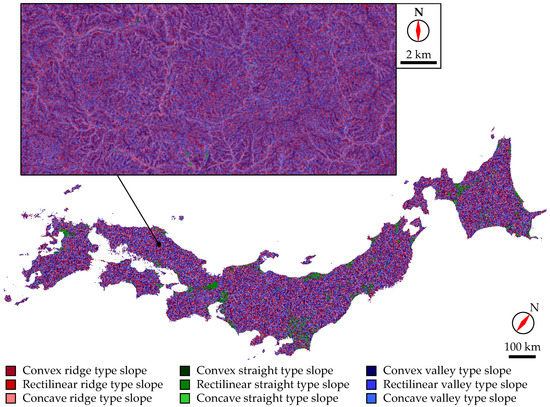
Figure 6. Slope type map of the Japanese archipelago.

3.2.4. Flow Accumulation

The flow accumulation was obtained by executing the creation tool of the flow accumulation raster in ArcGIS Pro. The flow accumulation is computed as the accumulated weight of all cells flowing into the cell in the descending slope of the reference cell. The calculated flow accumulation map is shown in Figure 7. The flow accumulation was classified into five classes by equal volume.

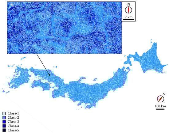
Figure 7. Flow accumulation map of the Japanese archipelago.

3.3. Geological Data

For the geological data, the 1/200,000 Japan Seamless Geological Map (basic version, data update date: 29 May 2015) [37] published by the National Institute of Advanced Industrial Science and Technology (AIST) was downloaded and used. Figure 8 shows the geological map of the Japanese archipelago converted into raster data using ArcGIS Pro. The geology of the Japanese archipelago is complicatedly distributed with mosaic patterns of plutonic (mainly granites), volcanic, and sedimentary rocks. In addition, many faults and active volcanoes exist, while adduct materials in which igneous and sedimentary rocks are complicatedly mixed, and metamorphic rocks of accretionary origin are also observed. In this study, the geology was divided into 27 sections as shown in Figure 8, considering geological age and lithofacies.

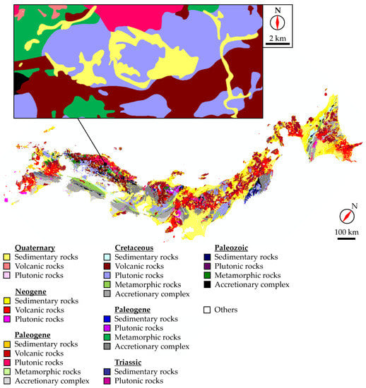
Figure 8. Geological map of the Japanese archipelago.

3.4. Vegetation data

For the vegetation data, the 1/50,000 existing vegetation map of GIS data (1979–1998) [38] published by the Biodiversity Center of Japan was downloaded and used. The download file is the same as the range of digital elevation model (DEM) data. The vegetation classification in Japan is largely divided into I to X. The vegetation map of the Japanese archipelago is shown in Figure 9. The plant distribution in the Japanese archipelago corresponds to temperature and precipitation, and with mountains exceeding 3000 m, the vegetation is distributed horizontally with latitude, and vertically by altitude [38].

Figure 9. Vegetation map of the Japanese archipelago.

4. Methods

The procedure of setting the evaluation factors and method in landslide susceptibility assessment is briefly explained. First, based on the landslide distribution map (Figure 1), the landslide topography of the Japanese archipelago was extracted, and the relationship between the landslide distribution and the evaluation factors/elements was statistically clarified. Next, based on these factors, a hierarchical system for landslide susceptibility assessment was constructed, as shown in Figure 10.

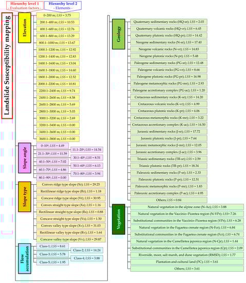
Figure 10. Hierarchy structure of the AHP for landslide susceptibility mapping. Characters in the parentheses are the abbreviations. LSS is landslide susceptibility score in Section 5.4.

From this hierarchical structure (Figure 10), the importance weights among each element (hierarchy level 2) were calculated, and then the importance weights among the evaluation factors (hierarchy level 1) were determined. In the AHP method, the criterion scale for the pairwise comparison in calculating the importance weights of evaluation factors (or elements) were “1: equal importance”, “3: moderate importance”, “5: strong importance”, “7: very strong importance”, and “9: absolute importance” (using 2, 4, 6, 8 complementarily), and the reciprocal if the importance was low. In other words, subjective and empirical judgments of the evaluator are required when using this scale. Therefore, statistical survey results of the relationship between landslide distribution and elements were introduced into a pair comparison of hierarchy level 2. Finally, the landslide susceptibility in each evaluation factor was scored from the importance weights of each hierarchy obtained by pairwise comparison. Thus, the total landslide susceptibility score was the sum of the corresponding landslide susceptibility score for each evaluation factor on a certain slope. If the total score was large, the landslide susceptibility was high, and if it was small, the landslide susceptibility was low. Then, landslide susceptibility mapping was performed by overlaying the landslide susceptibility scores of each evaluation factor using GIS (Figure 2). Moreover, by comparing the created susceptibility map with the landslide distribution, its suitability was examined, and landslide susceptibility assessment was conducted.

5. Relationship between Landslide Distribution and Evaluation Factors

In this section, the ratio (landslide area occupancy) of landslide topography to element division area in evaluation factors was obtained, and the relationship between evaluation factors and landslide distribution was described.

5.1. Relationship between Elevation and Landslide Distribution

The relationship between elevation and landslide distribution is shown in Figure 11. At elevations of 400–2000 m, the landslide area occupancy was approximately 7–8%, and there was no significant difference due to differences in elevation. At elevations of 2000 m or higher, the landslide area occupancy tended to decrease as the elevation increases, and landslide topography did not exist above 3200 m.

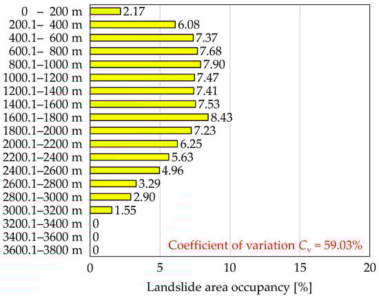
Figure 11. Relationship between landslide distribution and elevation. Abbreviations in this figure correspond to those used in Figure 10.

5.2. Relationship between Slope Angle and Landslide Distribution

The relationship between slope angle and landslide distribution is shown in Figure 12. The landslide area occupancy was the highest for slope angles ranging from 10.1–20°. Excluding the slope angle of 0–10°, the landslide area occupancy tended to decrease as the slope angle increased, and that landslide topography did not exist at slope angles greater than 81°.

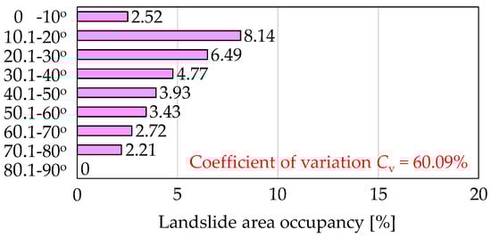
Figure 12. Relationship between landslide distribution and slope angle.

5.3. Relationship between Slope Type and Landslide Distribution

The relationship between slope type and landslide distribution is shown in Figure 13. In convex ridge (Xr), concave ridge (Vr), convex valley (Xv), and concave valley type slopes (Vv), no large difference in landslide area occupancy was observed, though they had a larger tendency to occur compared with other slope types. Therefore, the landslide topography was shown to have a close relationship with the slope type.

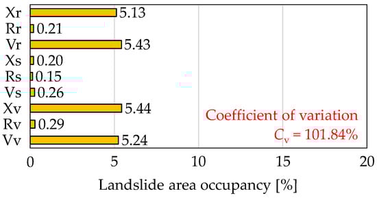
Figure 13. Relationship between landslide distribution and slope type. Abbreviations in this figure correspond to those used in Figure 10.

5.4. Relationship between Flow Accumulation and Landslide Distribution

The relationship between the flow accumulation and landslide distribution is shown in Figure 14. The landslide area occupancy was the highest in flow accumulation Class-2. With the exception of flow accumulation Class-1, the landslide area occupancy tended to decrease as the flow accumulation increased.

Figure 14. Relationship between landslide distribution and flow accumulation.

5.5. Relationship between Geology and Landslide Distribution

The relationship between geology and landslide distribution is shown in Figure 15. The landslide area occupancy was relatively large in the Neogene sedimentary and volcanic (N-sr, N-vr), Paleogene plutonic (PG-pr), Jurassic sedimentary (J-sr), and Triassic plutonic rocks (TR-pr). In other words, there was a tendency for landslide topography to exist in a particular geology, and there was a close relationship between the distribution of landslide topography and the geology.

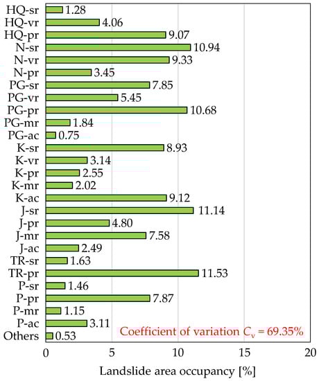
Figure 15. Relationship between landslide distribution and geology. Abbreviations in this figure correspond to those used in Figure 10.

5.6. Relationship between Vegetation and Landslide Distribution

The relationship between vegetation and landslide distribution is shown in Figure 16. The landslide area occupancy tended to be high in natural vegetation (N-VPr, N-Fcr) and substitutional communities in the Vaccinio–Piceetea (VPr) and Fagaetea crenate region (Fcr) distribution areas.

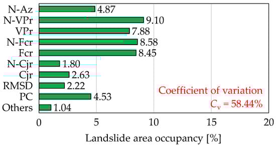
Figure 16. Relationship between landslide distribution and vegetation. Abbreviations in this figure correspond to those used in Figure 10.

6. Landslide Susceptibility Mapping Based on AHP Method

In this section, landslide susceptibility mapping in the whole slope of the Japanese archipelago was examined. Its evaluation factors were elevation, slope angle, slope type, flow accumulation, geology, and vegetation. The landslide susceptibility in the slope was evaluated with the score accumulation from the AHP method for these evaluation factors, and the landslide susceptibility map was prepared based on the landslide susceptibility level classified from I to V.

6.1. Outline of the AHP Method

The AHP method is an analytical decision-making method developed by Saaty [39]. It is used to determine the importance weights of evaluation items based on a pairwise comparison. For the evaluation factors and elements of landslide susceptibility assessment, the importance weights between the elements (hierarchy level 2) related to the evaluation factors were initially calculated from the hierarchical structure shown in Figure 10. Secondly, the importance weights among the higher evaluation factors (hierarchy level 1) were calculated. Finally, the landslide susceptibility level for each element was scored.

6.2. Pairwise Comparison between Elements (Hierarchy Level 2) and Calculation of Importance Weights

The criterion scales for pairwise comparisons in calculating the evaluation factors and the importance weights between elements were described in Section 3; however, when using this criterion scale, subjective and empirical judgment of engineers are required. Therefore, for this criterion scale, the results of the relationship between landslide distribution and evaluation factors obtained in Section 4 were introduced into a pair comparison of hierarchy level 2. That is, the ratio of pairwise comparing elements was used as a criterion scale to be consistent with the results of the relationship between landslide distribution and elements. Pairwise comparisons between elements (hierarchy level 2) related to the evaluation factors are shown in Table 1, Table 2, Table 3, Table 4, Table 5, Table 6, Table 7, Table 8 and Table 9 based on the results of the relationship between landslide area occupancy and elements.

Table 1. Pairwise comparisons of elements for elevation in hierarchy level 2 (e1–e19 vs. e1–e10). e1: 0–200 m, e2: 200.1–400 m, e3: 400.1–600 m, e4: 600.1–800 m, e5: 800.1–1000 m, e6: 1000.1–1200 m, e7: 1200.1–1400 m, e8: 1400.1–1600 m, e9: 1600.1–1800 m, e10: 1800.1–2000 m, e11: 2000.1–2200 m, e12: 2200.1–2400 m, e13: 2400.1–2600 m, e14: 2600.1–2800 m, e16: 2800.1–3000 m, e17: 3000.1–3200 m, e17: 3200.1–3400 m, e18: 3400.1–3600 m, e19: 3600.1–3800 m.

	e1	e2	e3	e4	e5	e6	e7	e8	e9	e10
e1	1	0.36	0.29	0.28	0.27	0.29	0.29	0.29	0.26	0.30
e2	2.81	1	0.83	0.79	0.77	0.81	0.82	0.81	0.72	0.84
e3	3.40	1.21	1	0.96	0.93	0.99	0.99	0.98	0.87	1.02
e4	3.54	1.26	1.04	1	0.97	1.03	1.04	1.02	0.91	1.06
e5	3.64	1.30	1.07	1.03	1	1.06	1.07	1.05	0.94	1.09
e6	3.44	1.23	1.01	0.97	0.95	1	1.01	0.99	0.89	1.03
e7	3.42	1.22	1.01	0.97	0.94	0.99	1	0.98	0.88	1.02
e8	3.47	1.24	1.02	0.98	0.95	1.01	1.02	1	0.89	1.04
e9	3.89	1.39	1.14	1.10	1.07	1.13	1.14	1.12	1	1.17
e10	3.33	1.19	0.98	0.94	0.92	0.97	0.98	0.96	0.86	1
e11	2.88	1.03	0.85	0.81	0.79	0.84	0.84	0.83	0.74	0.86
e12	2.59	0.92	0.76	0.73	0.71	0.75	0.76	0.75	0.67	0.78
e13	2.29	0.81	0.67	0.65	0.63	0.66	0.67	0.66	0.59	0.69
e14	1.52	0.54	0.45	0.43	0.42	0.44	0.44	0.44	0.39	0.45
e15	1.34	0.48	0.39	0.38	0.37	0.39	0.39	0.39	0.34	0.40
e16	0.72	0.26	0.21	0.20	0.20	0.21	0.21	0.21	0.18	0.21
e17	4.6 × 10−11	1.6 × 10−11	1.4 × 10−11	1.3 × 10−11	1.3 × 10−11	1.3 × 10−11	1.3 × 10−11	1.3 × 10−11	1.2 × 10−11	1.4 × 10−11
e18	4.6 × 10−11	1.6 × 10−11	1.4 × 10−11	1.3 × 10−11	1.3 × 10−11	1.3 × 10−11	1.3 × 10−11	1.3 × 10−11	1.2 × 10−11	1.4 × 10−11
e19	4.6 × 10−11	1.6 × 10−11	1.4 × 10−11	1.3 × 10−11	1.3 × 10−11	1.3 × 10−11	1.3 × 10−11	1.3 × 10−11	1.2 × 10−11	1.4 × 10−11

Table 2. Pairwise comparisons of elements for elevation in hierarchy level 2 (e1–e19 vs. e11–e19). Abbreviations in this table correspond to those used in Table 1.

	e11	e12	e13	e14	e15	e16	e17	e18	e19	Weight
e1	0.35	0.39	0.44	0.66	0.75	1.40	2.2 × 1010	2.2 × 1010	2.2 × 1010	2.31
e2	0.97	1.08	1.23	1.85	2.09	3.92	6.1 × 1010	6.1 × 1010	6.1 × 1010	6.48
e3	1.18	1.31	1.49	2.24	2.54	4.75	7.4 × 1010	7.4 × 1010	7.4 × 1010	7.86
e4	1.23	1.36	1.55	2.33	2.64	4.94	7.7 × 1010	7.7 × 1010	7.7 × 1010	8.18
e5	1.26	1.40	1.59	2.40	2.72	5.09	7.9 × 1010	7.9 × 1010	7.9 × 1010	8.42
e6	1.20	1.33	1.51	2.27	2.57	4.81	7.5 × 1010	7.5 × 1010	7.5 × 1010	7.96
e7	1.19	1.32	1.49	2.25	2.55	4.77	7.4 × 1010	7.4 × 1010	7.4 × 1010	7.90
e8	1.21	1.34	1.52	2.29	2.59	4.85	7.5 × 1010	7.5 × 1010	7.5 × 1010	8.03
e9	1.35	1.50	1.70	2.56	2.90	5.43	8.4 × 1010	8.4 × 1010	8.4 × 1010	8.99
e10	1.16	1.29	1.46	2.20	2.49	4.66	7.2 × 1010	7.2 × 1010	7.2 × 1010	7.71
e11	1	1.11	1.26	1.90	2.15	4.02	6.2 × 1010	6.2 × 1010	6.2 × 1010	6.65
e12	0.90	1	1.13	1.71	1.94	3.62	5.6 × 1010	5.6 × 1010	5.6 × 1010	5.99
e13	0.79	0.88	1	1.51	1.71	3.19	5.0 × 1010	5.0 × 1010	5.0 × 1010	5.28
e14	0.53	0.58	0.66	1	1.13	2.12	3.3 × 1010	3.3 × 1010	3.3 × 1010	3.50
e15	0.47	0.52	0.59	0.88	1	1.87	2.9 × 1010	2.9 × 1010	2.9 × 1010	3.09
e16	0.25	0.28	0.31	0.47	0.53	1	1.6 × 1010	1.6 × 1010	1.6 × 1010	1.65
e17	1.6 × 10−11	1.8 × 10−11	2.0 × 10−11	3.0 × 10−11	3.4 × 10−11	6.4 × 10−11	1	1.00	1.00	0.00
e18	1.6 × 10−11	1.8 × 10−11	2.0 × 10−11	3.0 × 10−11	3.4 × 10−11	6.4 × 10−11	1.00	1	1.00	0.00
e19	1.6 × 10−11	1.8 × 10−11	2.0 × 10−11	3.0 × 10−11	3.4 × 10−11	6.4 × 10−11	1.00	1.00	1	0.00

Table 3. Pairwise comparisons of elements for slope angle in hierarchy level 2. sa1: 0–10°, sa2: 10.1–20°, sa3: 20.1–30°, sa4: 30.1–40°, sa5: 40.1–50°, sa6: 50.1–60°, sa7: 60.1–70°, sa8: 70.1–80°, sa9: 80.1–90°.

	sa1	sa2	sa3	sa4	sa5	sa6	sa7	sa8	sa9	Weight
sa1	1	0.31	0.39	0.53	0.64	0.73	0.92	1.14	2.5 × 1010	7.36
sa2	3.24	1	1.25	1.71	2.07	2.37	2.99	3.69	8.1 × 1010	23.80
sa3	2.58	0.80	1	1.36	1.65	1.89	2.39	2.94	6.5 × 1010	18.98
sa4	1.89	0.59	0.73	1	1.21	1.39	1.75	2.16	4.8 × 1010	13.94
sa5	1.56	0.48	0.61	0.82	1	1.14	1.44	1.78	3.9 × 1010	11.49
sa6	1.36	0.42	0.53	0.72	0.87	1	1.26	1.56	3.4 × 1010	10.04
sa7	1.08	0.33	0.42	0.57	0.69	0.79	1	1.23	2.7 × 1010	7.96
sa8	0.88	0.27	0.34	0.46	0.56	0.64	0.81	1	2.2 × 1010	6.45
sa9	4.0 × 10−11	1.2 × 10−11	1.5 × 10−11	2.1 × 10−11	2.5 × 10−11	2.9 × 10−11	3.7 × 10−11	4.5 × 10−11	1	00.00

Table 4. Pairwise comparisons of elements for slope type in hierarchy level 2. st1: Convex ridge type slope, st2: Rectilinear ridge type slope, st3: Concave ridge type slope, st4: Convex straight type slope, st5: Rectilinear straight type slope, st6: Concave straight type slope, st7: Convex valley type slope, st8: Rectilinear valley type slope, st9: Concave valley type slope.

	st1	st2	st3	st4	st5	st6	st7	st8	st9	Weight
st1	1	24.84	0.94	25.18	33.30	19.46	0.94	17.89	0.98	22.95
st2	0.04	1	0.04	1.01	1.34	0.78	0.04	0.72	0.04	0.92
st3	1.06	26.29	1	26.65	35.24	20.59	1.00	18.93	1.04	24.28
st4	0.04	0.99	0.04	1	1.32	0.77	0.04	0.71	0.04	0.91
st5	0.03	0.75	0.03	0.76	1	0.58	0.03	0.54	0.03	0.69
st6	0.05	1.28	0.05	1.29	1.71	1	0.05	0.92	0.05	1.18
st7	1.06	26.36	1.00	26.71	35.33	20.64	1	18.98	1.04	24.35
st8	0.06	1.39	0.05	1.41	1.86	1.09	0.05	1	0.05	1.28
st9	1.02	25.37	0.97	25.72	34.01	19.87	0.96	18.27	1	23.44

Table 5. Pairwise comparisons of elements for flow accumulation in hierarchy level 2. f1: Class-1, f2: Class-2, f3: Class-3, f4: Class-4, f5: Class-5.

	f1	f2	f3	f4	f5	Weight
f1	1	0.61	1.49	2.22	4.43	25.00
f2	1.65	1	2.46	3.67	7.32	41.32
f3	0.67	0.41	1	1.49	2.97	16.77
f4	0.45	0.27	0.67	1	1.99	11.26
f5	0.23	0.14	0.34	0.50	1	5.65

Table 6. Pairwise comparisons of elements for geology in hierarchy level 2 (g1–e27 vs. g1–e10). g1: Quaternary sedimentary rocks, g2: Quaternary volcanic rocks, g3: Quaternary plutonic rocks, g4: Neogene sedimentary rocks, g5: Neogene volcanic rocks, g6: Neogene plutonic rocks, g7: Paleogene sedimentary rocks, g8: Paleogene sedimentary rocks, g9: Paleogene plutonic rocks, g10: Paleogene metamorphic rocks, g11: Paleogene accretionary complex, g12: Cretaceous sedimentary rocks, g13: Cretaceous volcanic rocks, g14: Cretaceous plutonic rocks, g15: Cretaceous metamorphic rocks, g16: Cretaceous accretionary complex, g17: Jurassic sedimentary rocks, g18: Jurassic plutonic rocks, g19: Jurassic metamorphic rocks, g20: Jurassic accretionary complex, g21: Triassic sedimentary rocks, g22: Triassic plutonic rocks, g23: Paleozoic sedimentary rocks, g24: Paleozoic plutonic rocks, g25: Paleozoic metamorphic rocks, g26: Paleozoic accretionary complex, g27: Others.

	g1	g2	g3	g4	g5	g6	g7	g8	g9	g10
g1	1	0.31	0.14	0.12	0.14	0.37	0.16	0.23	0.12	0.69
g2	3.18	1	0.45	0.37	0.43	1.18	0.52	0.75	0.38	2.21
g3	7.10	2.23	1	0.83	0.97	2.63	1.16	1.66	0.85	4.93
g4	8.57	2.70	1.21	1	1.17	3.17	1.39	2.01	1.02	5.95
g5	7.31	2.30	1.03	0.85	1	2.71	1.19	1.71	0.84	5.07
g6	2.70	0.85	0.38	0.32	0.37	1	0.44	0.63	0.32	1.87
g7	6.15	1.93	0.87	0.72	0.84	2.28	1	1.44	0.74	4.27
g8	4.27	1.34	0.60	0.50	0.58	1.58	0.69	1	0.51	2.96
g9	8.36	2.63	1.18	0.98	1.14	3.10	1.36	1.96	1	5.80
g10	1.44	0.45	0.20	0.17	0.20	0.53	0.23	0.34	0.17	1
g11	0.59	0.19	0.08	0.07	0.08	0.22	0.10	0.14	0.07	0.41
g12	6.99	2.20	0.98	0.82	0.96	2.59	1.14	1.64	0.84	4.85
g13	2.46	0.77	0.35	0.29	0.34	0.91	0.40	0.58	0.29	1.71
g14	2.00	0.63	0.28	0.23	0.27	0.74	0.33	0.47	0.24	1.39
g15	1.58	0.50	0.22	0.18	0.22	0.59	0.26	0.37	0.19	1.10
g16	7.14	2.25	1.01	0.83	0.98	2.65	1.16	1.67	0.85	4.96
g17	8.73	2.75	1.23	1.02	1.19	3.23	1.42	2.05	1.04	6.06
g18	3.76	1.18	0.53	0.44	0.51	1.39	0.61	0.88	0.45	2.61
g19	5.93	1.87	0.84	0.69	0.81	2.20	0.97	1.39	0.71	4.12
g20	1.95	0.61	0.27	0.23	0.27	0.72	0.32	0.46	0.23	1.35
g21	1.28	0.40	0.18	0.15	0.17	0.47	0.21	0.30	0.15	0.89
g22	9.03	2.84	1.27	1.05	1.24	3.35	1.47	2.12	1.08	6.27
g23	1.15	0.36	0.16	0.13	0.16	0.42	0.19	0.27	0.14	0.80
g24	6.16	1.94	0.87	0.72	0.84	2.28	1.00	1.44	0.74	4.28
g25	0.90	0.28	0.13	0.10	0.12	0.33	0.15	0.21	0.11	0.62
g26	2.44	0.77	0.34	0.28	0.33	0.90	0.40	0.57	0.29	1.69
g27	0.41	0.13	0.06	0.05	0.06	0.15	0.07	0.10	0.05	0.29

Table 7. Pairwise comparisons of elements for geology in hierarchy level 2 (g1–e27 vs. g11–e20). Abbreviations in this table correspond to those used in Table 6.

	g11	g12	g13	g14	g15	g16	g17	g18	g19	g20
g1	1.69	0.14	0.41	0.50	0.63	0.14	0.11	0.27	0.17	0.51
g2	5.38	0.45	1.29	1.59	2.01	0.44	0.36	0.84	0.54	1.63
g3	12.02	1.02	2.89	3.55	4.48	0.99	0.81	1.89	1.20	3.64
g4	14.51	1.23	3.49	4.29	5.41	1.20	0.98	2.28	1.44	4.39
g5	12.37	1.04	2.97	3.66	4.61	1.02	0.84	1.94	1.23	3.74
g6	4.57	0.39	1.10	1.35	1.70	0.38	0.31	0.72	0.46	1.38
g7	10.41	0.88	2.50	3.08	3.88	0.86	0.70	1.63	1.04	3.15
g8	7.22	0.61	1.74	2.13	2.69	0.60	0.49	1.13	0.72	2.19
g9	14.16	1.20	3.40	4.18	5.28	1.17	0.96	2.22	1.41	4.29
g10	2.44	0.21	0.59	0.72	0.91	0.20	0.17	0.38	0.24	0.74
g11	1	0.08	0.24	0.30	0.37	0.08	0.07	0.16	0.10	0.30
g12	11.84	1	2.84	3.50	4.41	0.98	0.80	1.86	1.18	3.58
g13	4.16	0.35	1	1.23	1.55	0.34	0.28	0.65	0.41	1.26
g14	3.38	0.29	0.81	1	1.26	0.28	0.23	0.53	0.34	1.02
g15	2.68	0.23	0.64	0.79	1	0.22	0.18	0.42	0.27	0.81
g16	12.09	1.02	2.91	3.57	4.51	1	0.82	1.90	1.20	3.66
g17	14.78	1.25	3.55	4.37	5.51	1.22	1	2.32	1.47	4.47
g18	6.37	0.54	1.53	1.88	2.37	0.53	0.43	1	0.63	1.93
g19	10.05	0.85	2.41	2.97	3.74	0.83	0.68	1.58	1	3.04
g20	3.30	0.28	0.79	0.98	1.23	0.27	0.22	0.52	0.33	1
g21	2.16	0.18	0.52	0.64	0.81	0.18	0.15	0.34	0.22	0.65
g22	15.30	1.29	3.68	4.52	5.70	1.26	1.03	2.40	1.52	4.63
g23	1.94	0.16	0.47	0.57	0.72	0.16	0.13	0.30	0.19	0.59
g24	10.43	0.88	2.51	3.08	3.89	0.86	0.71	1.64	1.04	3.16
g25	1.52	0.13	0.37	0.45	0.57	0.13	0.10	0.24	0.15	0.46
g26	4.13	0.35	0.99	1.22	1.54	0.34	0.28	0.65	0.41	1.25
g27	0.70	0.06	0.17	0.21	0.26	0.06	0.05	0.11	0.07	0.21

Table 8. Pairwise comparisons of elements for geology in hierarchy level 2 (g1–e27 vs. g21–e27). Abbreviations in this table correspond to those used in Table 6.

	g21	g22	g23	g24	g25	g26	g27	Weight
g1	0.78	0.11	0.87	0.16	1.11	0.41	2.43	0.89
g2	2.49	0.35	2.77	0.52	3.53	1.30	7.71	2.82
g3	5.56	0.79	6.20	1.15	7.90	2.91	17.22	6.31
g4	6.71	0.95	7.48	1.39	9.53	3.51	20.78	7.61
g5	5.72	0.81	6.38	1.19	8.12	3.00	17.72	6.49
g6	2.11	0.30	2.36	0.44	3.00	1.11	6.55	2.40
g7	4.81	0.68	5.37	1.00	6.84	2.52	14.91	5.46
g8	3.34	0.47	3.72	0.69	4.74	1.75	10.34	3.79
g9	6.55	0.93	7.30	1.36	9.30	3.43	20.28	7.43
g10	1.13	0.16	1.26	0.23	1.60	0.59	3.49	1.28
g11	0.46	0.07	0.52	0.10	0.66	0.24	1.43	0.52
g12	5.48	0.77	6.10	1.14	7.77	2.87	16.96	6.21
g13	1.93	0.27	2.15	0.40	2.73	1.01	5.96	2.18
g14	1.57	0.22	1.74	0.32	2.22	0.82	4.85	1.78
g15	1.24	0.18	1.38	0.26	1.76	0.65	3.84	1.41
g16	5.59	0.79	6.23	1.16	7.94	2.93	17.32	6.34
g17	6.84	0.97	7.62	1.42	9.70	3.58	21.17	7.75
g18	2.95	0.42	3.28	0.61	4.18	1.54	9.12	3.34
g19	4.65	0.66	5.18	0.96	6.60	2.43	14.39	5.27
g20	1.53	0.22	1.70	0.32	2.17	0.80	4.73	1.73
g21	1	0.14	1.11	0.21	1.42	0.52	3.10	1.13
g22	7.07	1	7.88	1.47	10.04	3.70	21.91	8.02
g23	0.90	0.13	1	0.19	1.27	0.47	2.78	1.02
g24	4.82	0.68	5.38	1	6.85	2.53	14.94	5.47
g25	0.70	0.10	0.78	0.15	1	0.37	2.18	0.80
g26	1.91	0.27	2.13	0.40	2.71	1	5.91	2.17
g27	0.32	0.05	0.36	0.07	0.46	0.17	1	0.37

Table 9. Pairwise comparisons of elements for vegetation in hierarchy level 2. v1: Natural vegetation in the alpine zone, v2: Natural vegetation in the Vaccinio–Piceetea region, v3: Substitutional communities in the Vaccinio–Piceetea region, v4: Natural vegetation in the Fagaetea crenate region, v5: Substitutional communities in the Fagaetea crenate region, v6: Natural vegetation in the Camellietea japonica region, v7: Substitutional communities in the Camellietea japonica region, v8: Riverside, moor, salt marsh, and dune vegetation, v9: Plantation and cultural land, v10: Others.

	v1	v2	v3	v4	v5	v6	v7	v8	v9	v10	Weight
v1	1	0.53	0.62	0.57	0.58	2.70	1.85	2.19	1.08	4.66	9.52
v2	1.87	1	1.16	1.06	1.08	5.05	3.46	4.09	2.01	8.71	17.81
v3	1.62	0.87	1	0.92	0.93	4.37	3.00	3.54	1.74	7.54	15.42
v4	1.76	0.94	1.09	1	1.02	4.76	3.27	3.86	1.90	8.21	16.79
v5	1.74	0.93	1.07	0.99	1	4.69	3.22	3.80	1.87	8.09	16.54
v6	0.37	0.20	0.23	0.21	0.21	1	0.69	0.81	0.40	1.73	3.53
v7	0.54	0.29	0.33	0.31	0.31	1.46	1	1.18	0.58	2.51	5.14
v8	0.46	0.24	0.28	0.26	0.26	1.23	0.85	1	0.49	2.13	4.35
v9	0.93	0.50	0.57	0.53	0.54	2.51	1.72	2.03	1	4.33	8.86
v10	0.21	0.11	0.13	0.12	0.12	0.58	0.40	0.47	0.23	1	2.04

The paired comparisons between the elements (hierarchical level 2) related to the evaluation factors are explained using the “elevation” in Table 1 and Table 2 as an example. The value of the pairwise comparison between “elevation 200.1-” (landslide area occupancy = 6.08%: Figure 11) and “elevation 0-” (landslide area occupancy = 2.17%: Figure 11) was 6.08%/2.17% = 2.81 (Table 1 and Table 2). The reciprocal (0.36) was obtained by the pairwise comparison between “elevation 0-” and “elevation 200.1-” (Table 1 and Table 2). However, since the geometric averaging method was used to calculate the importance weights, if no landslide topography was identified, the landslide area occupancy in the element was calculated as 1.0 × 10⁻¹⁰ instead of 0 in the ratio between elements (Table 1 and Table 2). Moreover, the consistency of pairwise comparison was evaluated using the consistency index (C.I.). When C.I. = 0, it is completely consistent, and when C.I. < 0.10 to 0.15, it is consistent [39]. The ratio between the elements to be paired was used; thus, naturally C.I. = 0. The ranking of the importance weights of “elevation” (Table 1 and Table 2) corresponds to the ranking in Figure 11.

6.3. Pairwise Comparison between Evaluation Factors (Hierarchy Level 1) and Calculation of Importance Weights

As mentioned in Section 5.2., a pairwise comparison between evaluation factors (hierarchy level 1) was performed to calculate the importance weights. In this study, however, the criterion scale for pairwise comparisons between evaluation factors at hierarchy level 1 was determined based on the coefficient of variation for importance weights at hierarchy level 2. The coefficient of variation is an indicator of the data dispersion; however, if the dispersion of the importance weights of the elements at hierarchy level 2 was large, the landslide topography was concentrated and distributed on a specific element. In other words, there was a significant relationship between the evaluation factors and the landslide distribution. Naturally, the relationship with the landslide distribution was also low, and the coefficient of variation was also 0, if all degrees of importance among the elements in the hierarchy level 2 were the same. A pairwise comparison between evaluation factors (hierarchy level 1) is shown in Table 10. The numerical value of the pairwise comparison between the “slope angle” and “elevation” (1.02) was taken as an example. Firstly, the coefficient of variation for the importance weight of the slope angle was calculated as 60.09% from Figure 12. Similarly, the coefficient of variation for elevation was calculated as 59.03% from Figure 11. Comparing the coefficients of variation between the two factors, the value of “slope angle” was larger than that of “elevation”, and the dispersion was large; thus, the importance was higher with respect to landslide susceptibility evaluation. Similar to the pairwise comparison at hierarchy level 2, the value of the pairwise comparison was set to 1.02 by using the ratio (60.09%/59.03%) of both values.

Table 10. Pairwise comparisons of evaluation factors in hierarchy level 1.

	El	SAng	STyp	Flow	Geol	Veg	Weight
Elevation (El)	1	0.98	0.58	0.95	0.85	1.01	14.60
Slope angle (SAng)	1.02	1	0.59	0.97	0.87	1.03	14.54
Slope type (STyp)	1.73	1.69	1	1.64	1.47	1.74	31.03
Flow accumulation (Flow)	1.05	1.03	0.61	1	0.90	1.06	14.23
Geology (Geol)	1.17	1.15	0.68	1.12	1	1.19	18.34
Vegetation (Veg)	0.99	0.97	0.57	0.94	0.84	1	7.26

6.4. Calculation of Landslide Susceptibility Score

From the importance weights of each hierarchy (evaluation factors and elements), the landslide susceptibility score (LSS) in each element for each evaluation factor was calculated using the following Equation (6):

$$LSS=\frac{W_1{W}_2}{W_{2\mathrm{MAX}}}$$

(6)

where W₁ is the importance weight of each evaluation factor in hierarchy level 1, W₂ is the importance weight of each element in hierarchy level 2, and W_2MAX is the highest value of the importance weight of each element in hierarchy level 2. In Equation (6), the total LSS is 100; however, the highest score of the element in the evaluation factor became the same value as the importance weight of the evaluation factor (hierarchy level 1). For example, LSS at “elevation 0 to 200 m” was calculated as 3.75 scores: W₁ = 14.60 (Table 10), W₂ = 2.31, and W_2MAX = 8.99 (Table 1 and Table 2). As “elevation 1600.1–1800 m” had the largest importance weight among the elements of “elevation”, LSS (=14.60) coincided with the importance weight (14.60) of “elevation” in hierarchy level 1. Figure 10 shows LSS for each element related to the evaluation factors.

6.5. Results and Discussion of Landslide Susceptibility Mapping

On a certain slope (cell of 20 m × 20 m), the total LSS (superimposed using GIS) corresponding to each evaluation factor was taken as the total LSS. Landslide susceptibility mapping was performed based on the susceptibility level classified from I to V. If the total score was large, the landslide susceptibility was high, and if it was small, the landslide susceptibility was low. Landslide susceptibility levels I to V divided the total score of 100 scores into intervals of 20.

A landslide susceptibility map for the Japanese archipelago is shown in Figure 17. In this map, landslide susceptibility level IV distribution area occupies approximately half of the map, and landslide susceptibility level V distribution area occupies approximately 30%. The hazard rank IV distribution area also occupies approximately half of the map, and the hazard rank V distribution area occupies approximately 30%. Landslide susceptibility level I distribution area is practically nonexistent, and landslide susceptibility level II and III distribution areas are primarily distributed in coastal and plain areas.

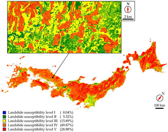
Figure 17. Landslide susceptibility map of the Japanese archipelago.

Subsequently, the relationship between landslide susceptibility map and distribution is shown in Figure 18. This study discusses the suitability of the landslide susceptibility map and distributions in the Japanese archipelago, confirming the LSS distribution and landslide occurrence rate, such as whether landslide topography is concentrated in the high scoring area, and whether landslides are not occurring in the low score area. When to the relationship between landslide susceptibility level and landslide area occupancy is examined (Figure 18), the landslide area occupancy tends to increase as landslide susceptibility increases. Thus, a consistent relationship exists between landslide susceptibility level and distribution. Therefore, the landslide susceptibility map created by this method expresses the past landslide distribution well. Our method can be applied to the extraction of unstable slopes, and is effective for prioritizing regions and implementing efficient countermeasures.

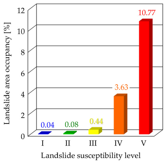
Figure 18. Relationship between landslide susceptibility level and distribution in the landslide susceptibility map shown in Figure 17.

Finally, the receiver operating characteristic (ROC) curves and area under the curve (AUC) values [40] were used to validate the landslide hazard map in this study. ROC curves and AUC values are often used to validate landslide hazard maps, e.g., [33,41,42,43,44]. Figure 19 illustrates the ROC curve representing the relationship between the landslide hazard map (Figure 17) and landslide distribution. The curve plots the false (i.e., 1-specificity) and true (sensitivity) positive rates on the horizontal and vertical axes, respectively. More values closer to the upper left (the point at which low false and high true positive rates are achieved simultaneously) imply better models. The AUC value indicates the quality of the evaluation method, and ranges from 0–1. The closer it is to 1, the higher the discrimination ability. A value of 1 indicates that perfect classification is possible, whereas 0.5 indicates random classification. In general, the criteria for AUC values are as follows: 0.9–1.0: excellent, 0.8–0.9: good, 0.7–0.8: fair, 0.6–0.7: poor, and 0.5–0.6: failure. In this study, the AUC value of the evaluation method was 0.86, which is a relatively high value. Furthermore, it can be inferred that it is as high as that in previous studies [33,41,42,43,44] on landslide hazard mapping using AHP and GIS. Therefore, results in this study have the ability to classify landslide hazards. In contrast, the analysis target range included a very wide area of the entire Japanese Archipelago in this study. Therefore, the analysis time was long. Moreover, the Japanese Archipelago has a complex geological and vegetation environment, making it necessary to discuss the setting of the analysis target range. This should be examined in future research.

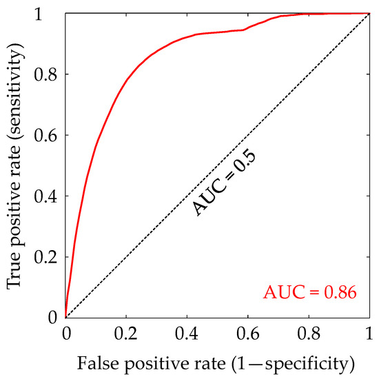
Figure 19. ROC curves and AUC values for the AHP model in this study.

7. Conclusions

We investigated the landslide susceptibility assessment method in the Japanese archipelago using the AHP method and GIS analysis based on the landslide topography of the Japanese archipelago, which covers approximately 370,000 locations. Then, we extracted slopes with the same degree of hazard/risk as areas where past landslides occurred. Thus, a consistent relationship was obtained between the created landslide susceptibility map and landslide distribution. Furthermore, from the AUC value of the evaluation method, it can be inferred that it is as high as that in previous studies on landslide hazard mapping using AHP and GIS. Therefore, results in this study have the ability to classify landslide hazards, and this method can extract unstable slopes and contribute to the development of efficient measures for the appropriate regions and slope disaster prevention technology. In particular, the method in this study is based on the existing AHP method and GIS. However, this AHP method is considered to be one step ahead of existing evaluation methods using the AHP method, by introducing the statistical survey results of landslide topography and evaluation factors/elements. A further advantage of this method is that the analysis can be performed using only free available data.

Despite been evaluated as having a low landslide susceptibility level, there are some places where landslides and recent slope disasters have occurred. Thus, we plan to conduct field surveys and field/laboratory experiments to examine the accuracy, applicability, and practical application of this method. In addition, we plan to further improve this method by fusing the current data with rainfall and earthquake data, a 3D ground structure model for seismic motion evaluation by geophysical exploration, and landslide scenarios generated by numerical analysis and the event tree method.

References

- Japan Sabo Association. Handbook of Sabo; Japan Sabo Association: Tokyo, Japan, 2015; pp. 1–708. (In Japanese) [Google Scholar]
- Digital archive for Landslide Distribution Maps, National Research Institute for Earth Science and Disaster Resilience (NIED). Available online: https://dil-opac.bosai.go.jp/publication/nied_tech_note/landslidemap/gis.html (accessed on 1 April 2021).
- Fujiwara, O.; Yanagida, M.; Shimizu, N.; Sanga, T.; Sasaki, T. Regional distribution of large landslide landforms in Japan—Implication in geology and landform. J. Jpn. Landslide Soc. 2004, 41, 335–344. (In Japanese) [Google Scholar] [CrossRef] [PubMed]
- Araiba, K.; Nozaki, T.; Jeong, B.; Fukumoto, Y. Distribution of landslides and their geological characteristics in Japan—Analysis report based on the data of nation-wide designated landslide-threatened areas. J. Jpn. Landslide Soc. 2008, 44, 318–323. (In Japanese) [Google Scholar] [CrossRef]
- Maeda, H.; Oguchi, N.; Matsumoto, N. Slide hazard mapping of Kanehana landslide area in Rubeshibe, northeastern Hokkaido, Japan. J. Jpn. Landslide Soc. 2001, 38, 61–68. (In Japanese) [Google Scholar] [CrossRef]
- Moriwaki, H.; Sasaki, Y. Relative risk evaluation of old landslides with slope stability analysis. J. Jpn. Landslide Soc. 2007, 44, 25–32. (In Japanese) [Google Scholar] [CrossRef]
- Lee, S.; Pradhan, B. Landslide hazard mapping at Selangor, Malaysia using frequency ratio and logistic regression models. Landslides 2007, 4, 33–41. [Google Scholar] [CrossRef]
- Jiménez-Perálvarez, J.D.; El Hamdouni, R.; Palenzuela, J.A.; Irigaray, C.; Chacón, J. Landslide-hazard mapping through multi-technique activity assessment: An example from the Betic Cordillera (southern Spain). Landslides 2017, 14, 1975–1991. [Google Scholar] [CrossRef]
- Bera, A.; Mukhopadhyay, B.P.; Das, D. Landslide hazard zonation mapping using multi-criteria analysis with the help of GIS techniques: A case study from Eastern Himalayas, Namchi, South Sikkim. Nat. Hazards 2019, 96, 935–959. [Google Scholar] [CrossRef]
- Xu, S.; Zhang, M.; Ma, Y.; Liu, J.; Wang, Y.; Ma, X.; Chen, J. Multiclassification method of landslide risk assessment in consideration of disaster levels: A case study of Xianyang City, Shaanxi Province. ISPRS Int. J. Geo-Inf. 2021, 10, 646. [Google Scholar] [CrossRef]
- Batar, A.K.; Watanabe, T. Landslide susceptibility mapping and assessment using geospatial platforms and weights of evidence (WoE) method in the Indian Himalayan region: Recent developments, gaps, and future directions. ISPRS Int. J. Geo-Inf. 2021, 10, 114. [Google Scholar] [CrossRef]
- Nagata, H.; Sakaguchi, T.; Kojima, S. Analysis of topographic and geologic factors in unstable slope distribution using GIS. J. Jpn. Soc. Eng. Geol. 2006, 46, 320–330. (In Japanese) [Google Scholar] [CrossRef]
- Zhou, G.; Yokoya, N.; Cheng, G.; Kitazono, Y. An advanced slope failure hazard mapping method by combing GIS and Hayashi’s quantification methods theory. J. Jpn. Soc. Eng. Geol. 2008, 49, 2–12. (In Japanese) [Google Scholar] [CrossRef]
- Pandey, A.; Shahbodaghlou, F. Landslide hazard mapping of Nagadhunga-Naubise section of the Tribhuvan highway in Nepal with GIS Application. J. Geogr. Inf. Syst. 2014, 6, 723–732. [Google Scholar] [CrossRef]
- Hamasaki, E.; Higaki, D.; Hayashi, K. Buffer movement analysis and blunder probability analysis for GIS-based landslide susceptibility mapping—A case study of the 2008 Iwate-Miyagi Nairiku Earthquake, Japan. J. Jpn. Landslide Soc. 2015, 52, 51–59. (In Japanese) [Google Scholar] [CrossRef]
- Marana, B. A simplified ArcGIS approach for landslides risk assessment in the Province of Bergamo. J. Geogr. Inf. Syst. 2017, 9, 699–716. [Google Scholar] [CrossRef]
- Mersha, T.; Meten, M. GIS-based landslide susceptibility mapping and assessment using bivariate statistical methods in Simada area, northwestern Ethiopia. Geoenviron. Disasters 2020, 7, 20. [Google Scholar] [CrossRef]
- Moresi, F.V.; Maesano, M.; Collalti, A.; Sidle, R.C.; Matteucci, G.; Scarascia Mugnozza, G. Mapping landslide prediction through a GIS-based model: A case study in a catchment in Southern Italy. Geosciences 2020, 10, 309. [Google Scholar] [CrossRef]
- Shahabi, H.; Hashim, M. Landslide susceptibility mapping using GIS-based statistical models and remote sensing data in tropical environment. Sci. Rep. 2015, 5, 9899. [Google Scholar] [CrossRef]
- Psomiadis, E.; Charizopoulos, N.; Efthimiou, N.; Soulis, K.X.; Charalampopoulos, I. Earth observation and GIS-based analysis for landslide susceptibility and risk assessment. ISPRS Int. J. Geo-Inf. 2020, 9, 552. [Google Scholar] [CrossRef]
- Han, L.; Zhang, J.; Zhang, Y.; Ma, Q.; Alu, S.; Lang, Q. Hazard assessment of earthquake disaster chains based on a Bayesian Network model and ArcGIS. ISPRS Int. J. Geo-Inf. 2019, 8, 210. [Google Scholar] [CrossRef]
- Miyagi, T.; Prasad, G.B.; Tanavud, C.; Potichan, A.; Hamasaki, E. Landslide risk evaluation and mapping -Manual of aerial photo interpretation for landslide topography and risk management. In Report of the National Research Institute for Earth Science and Disaster Prevention; National Research Institute for Earth Science and Disaster Resilience: Tsukuba, Japan, 2004; pp. 75–137. [Google Scholar]
- Yoshimatsu, H.; Abe, S. A review of landslide hazards in Japan and assessment of their susceptibility using an analytical hierarchic process (AHP) method. Landslides 2006, 3, 149–158. [Google Scholar] [CrossRef]
- Yagi, H.; Higaki, D.; JLS Research Committee for Detection of Landslide Hazardous Sites in Tertiary Distributed Area. Methodological study on landslide hazard assessment by interpretation of aerial photographs combined with AHP in the middle course area of Agano River, Central Japan. J. Jpn. Landslide Soc. 2009, 45, 358–366. (In Japanese) [Google Scholar] [CrossRef]
- Hasekioğulları, G.D.; Ercanoglu, M. A new approach to use AHP in landslide susceptibility mapping: A case study at Yenice (Karabuk, NW Turkey). Nat. Hazards 2012, 63, 1157–1179. [Google Scholar] [CrossRef]
- Kohno, M.; Maeda, H. Experiment on landslide hazard mapping, based on AHP method, in consideration of point load strength of hydrothermally altered rock: Example in the Ohekisawa-Shikerebenbetsugawa landslide area, Japan. J. Jpn. Landslide Soc. 2013, 50, 121–129. (In Japanese) [Google Scholar] [CrossRef]
- Geologocal Survey of Hokkaido. Special Report of the Geologocal Survey of Hokkaido; Geologocal Survey of Hokkaido: Hokkaido, Japan, 2013; pp. 1–119. (In Japanese) [Google Scholar]
- Hung, L.Q.; Van, N.T.H.; Duc, D.M.; Ha, L.T.C.; Son, P.V.; Khanh, N.H.; Binh, L.T. Landslide susceptibility mapping by combining the analytical hierarchy process and weighted linear combination methods: A case study in the upper Lo River catchment (Vietnam). Landslides 2016, 13, 1285–1301. [Google Scholar] [CrossRef]
- Myronidis, D.; Papageorgiou, C.; Theophanous, S. Landslide susceptibility mapping based on landslide history and analytic hierarchy process (AHP). Nat. Hazards 2016, 81, 245–263. [Google Scholar] [CrossRef]
- Rahim, I.; Ali, S.; Aslam, M. GIS based landslide susceptibility mapping with application of analytical hierarchy process in district Ghizer, Gilgit Baltistan Pakistan. J. Geosci. Environ. Protect. 2018, 6, 34–49. [Google Scholar] [CrossRef]
- Kohno, M.; Noguchi, T.; Nishimura, T. Landslide hazard mapping in the Chugoku Region using AHP method and GIS. J. Jpn. Landslide Soc. 2020, 57, 3–11. (In Japanese) [Google Scholar] [CrossRef]
- Panchal, S.; Shrivastava, A.K. A Comparative study of frequency ratio, Shannon’s entropy and analytic hierarchy process (AHP) models for landslide susceptibility assessment. ISPRS Int. J. Geo-Inf. 2021, 10, 603. [Google Scholar] [CrossRef]
- Rehman, A.; Song, J.; Haq, F.; Mahmood, S.; Ahamad, M.I.; Basharat, M.; Sajid, M.; Mehmood, M.S. Multi-hazard susceptibility assessment using the analytical hierarchy process and frequency ratio techniques in the northwest Himalayas, Pakistan. Remote Sens. 2022, 14, 554. [Google Scholar] [CrossRef]
- Kohno, M.; Higuchi, Y.; Ono, Y. Evaluating earthquake-induced widespread slope failure hazards using an AHP-GIS combination. Nat. Hazards 2022, 1–28. [Google Scholar] [CrossRef]
- Digital Elevation Model (DEM10B), Geospatial Information Authority of Japan (GSI). Available online: https://fgd.gsi.go.jp/download/menu.php (accessed on 1 April 2021).
- Suzuki, T. Introduction to Map Reading for Civil Engineers Volume l—Geomorphological Basis for Map Reading; Kokon Shoin: Tokyo, Japan, 1997; pp. 122–124. (In Japanese) [Google Scholar]
- Seamless Digital Geological Map of Japan (1:200,000) (Basic version, data update date: 29 May 2015), National Institute of Advanced Industrial Science and Technology (AIST). Available online: https://gbank.gsj.jp/seamless/index_en.html (accessed on 1 April 2021).
- The Natural Environmental Information GIS, Ministry of the Environment Government of Japan (MOE). Available online: https://www.biodic.go.jp/trialSystem/top_en.html (accessed on 1 April 2021).
- Saaty, T.L. The Analytic Hierarchy Process; McGraw-Hill Int. Book Co.: New York, NY, USA, 1980; pp. 1–287. [Google Scholar]
- Fawcett, T. An introduction to ROC analysis. Pattern Recogn. Lett. 2016, 27, 861–874. [Google Scholar] [CrossRef]
- Sun, X.; Chen, J.; Bao, Y.; Han, X.; Zhan, J.; Peng, W. Landslide Susceptibility Mapping Using Logistic Regression Analysis along the Jinsha River and Its Tributaries Close to Derong and Deqin County, Southwestern China. ISPRS Int. J. Geo-Inf. 2018, 7, 438. [Google Scholar] [CrossRef]
- Meena, S.R.; Ghorbanzadeh, O.; Blaschke, T. A Comparative Study of Statistics-Based Landslide Susceptibility Models: A Case Study of the Region Affected by the Gorkha Earthquake in Nepal. ISPRS Int. J. Geo-Inf. 2019, 8, 94. [Google Scholar] [CrossRef]
- Senouci, R.; Taibi, N.-E.; Teodoro, A.C.; Duarte, L.; Mansour, H.; Yahia Meddah, R. GIS-Based Expert Knowledge for Landslide Susceptibility Mapping (LSM): Case of Mostaganem Coast District, West of Algeria. Sustainability 2021, 13, 630. [Google Scholar] [CrossRef]
- Kincal, C.; Kayhan, H. A Combined Method for Preparation of Landslide Susceptibility Map in Izmir (Türkiye). Appl. Sci. 2022, 12, 9029. [Google Scholar] [CrossRef]
Disclaimer/Publisher’s Note: The statements, opinions and data contained in all publications are solely those of the individual author(s) and contributor(s) and not of MDPI and/or the editor(s). MDPI and/or the editor(s) disclaim responsibility for any injury to people or property resulting from any ideas, methods, instructions or products referred to in the content. |
© 2023 by the authors. Licensee MDPI, Basel, Switzerland. This article is an open access article distributed under the terms and conditions of the Creative Commons Attribution (CC BY) license (https://creativecommons.org/licenses/by/4.0/).