Tour-Route-Recommendation Algorithm Based on the Improved AGNES Spatial Clustering and Space-Time Deduction Model

Abstract

This study designed a tour-route-planning and recommendation algorithm that was based on an improved AGNES spatial clustering and space-time deduction model. First, the improved AGNES tourist attraction spatial clustering algorithm was created. Based on the features and spatial attributes, city tourist attraction clusters were formed, in which the tourist attractions with a high degree of correlation among attributes were gathered into the same cluster. It formed the precondition for searching tourist attractions that would match tourist interests. Using tourist attraction clusters, this study also developed a tourist attraction reachability model that was based on tourist-interest data and geospatial relationships to confirm each tourist attraction’s degree of correlation to tourist interests. A dynamic space-time deduction algorithm that was based on travel time and cost allowances was designed in which the transportation mode, time, and costs were set as the key factors. To verify the proposed algorithm, two control algorithms were chosen and tested against the proposed algorithm. Our results showed that the proposed algorithm had better results for tour-route planning under different transportation modes as compared to the controls. The proposed algorithm not only considered time and cost allowances, but it also considered the shortest traveling distance between tourist attractions. Therefore, the tourist attractions and tour routes that were suggested not only met tourist interests, but they also conformed to the constraint conditions and lowered the overall total costs.

1. Introduction

Tourists are the core of tourism activity. A key issue of smart tourism is how to improve tourist satisfaction and provide the best experience. A complete tourism activity cycle includes pre-travel, traveling, and post-travel activities. The pre-travel experience includes itinerary, planning, and tour-route searching, etc. The travel process itself includes visiting tourist attractions and the travel between locations, etc. The post-travel activity includes the evaluation and feedback on the tourism experience as a whole. In the whole tourism activity cycle, the pre-travel experience is the most important factor to influence tourists’ satisfaction and, therefore, their subjective evaluations regarding the quality of their experiences. Tourists will have spent a certain amount of time and cost on their experiences. Therefore, devising and suggesting tour routes according to tourists’ needs and desires while realizing the minimum time and cost as well as the maximum benefit is key to optimal tour planning.

In a tour, the tourism objects are tourist attractions. Searching the very tourist attractions that accurately match the tourists’ needs is the critical step for the planning and recommending of tour routes. Tourists’ needs have large discrepancies, while the tourist attractions distributed in a city also have different feature attributes and spatial attributes, for which reason, each tourist attraction has relatively large different capacities on meeting tourists’ needs. The diversity of tourists’ needs and tourist attractions’ attributes makes the searching process complex. Thus, rapidly confirming the interested tourist attraction groups according to the tourists’ needs can improve the searching algorithm’s accuracy and efficiency, so that applying the effective method to generate tourist attraction groups is the key step to search the accurate tourist attractions. In data mining technology, a clustering algorithm can group spatial dots. It absorbs the spatial dots which have the similar attributes into the same group and divides the large scale data mining into a smaller scale one in the group, which can improve the algorithm efficiency. This paper uses the clustering algorithm to generate city tourist attraction clusters in accordance with tourist attraction attributes, and it provides the algorithm basis for searching accurate tourist attractions. There are many kinds of clustering algorithms. This paper uses AGNES as the basic algorithm to set up the clustering model. The agglomerative nesting (AGNES) algorithm is a hierarchical clustering method that operates from bottom to top. It sets the elements as the bottom layer in the spatial distribution and gathers them from bottom to top according to a defined criterion. The AGNES algorithm is a single-link method where each cluster is represented by its arbitrary elements. Therefore, the degree of correlation of two clusters is determined by the two values with the highest degree of correlation in each cluster. The clustering process begins at the discrete distributed bottom layer and gathers each dot within the clusters and ends with the preset number of clusters. A traditional AGNES algorithm is operated with the same spatial distance as the criterion. The reasons for this paper to use AGNES are as follows. First, AGNES is simple and it is easy to implement. AGNES is a naive clustering algorithm, which has a concise principle and process. Its starting and ending conditions are definite and the selecting of the starting seed point is simple. In the clustering process, it only needs to judge the dispersion between the seed point and the non-seed point. Compared with other clustering algorithms, it is more accessible and easier to implement. Second, AGNES has relatively low spatial complexity and time complexity. It has a faster operating rate and consumes less computer memory. Third, AGNES is very suitable for the clustering on small scale dataset. In this paper, the research objects are city tourist attractions; it forms a typical small scale dataset, thus the AGNES is feasible. Fourth, AGNES is more flexible and can realize the multiple layer clustering structures on different granularity by setting different parameters. It has no strict requirements on the samples inputting sequence and can realize the synchronous clustering from different dots to reduce the convergence time.

In tourism clustering research, [1] provided a general introduction on the clustering method, including the AGNES clustering algorithm. In [2], the researchers applied the hierarchical cluster analysis to a set of Indonesian tourism sites in and around Malang City, Malang Regency, and Batu City using the AGNES algorithm to optimize a search engine that could assist tourists when choosing tourist attractions under certain constraints. In another study [3], the AGNES algorithm was applied to the data from the online platform, Airbnb. The collaborative economy of tourism hosts based on their geographic distribution was studied. The city of Guanajuato, Mexico, was selected as the subject city for convenience purposes, and the main touristic attractions were used as parameters to conduct the analysis. According to [4], an ontology-based clustering method was used to analyze the qualitative factors from a semantic perspective to define tourist segments and understand why tourists travelled to a particular destination in the Catalonia region of Spain, and the researchers reported better results using this method as compared to classic clustering algorithm methods. In the literature, the proposed ontology-based clustering method was derived from an extension of the AGNES clustering algorithm. Researchers in [5] designed an original approach to characterize the daily behaviors of tourists by analyzing the sequences of places that were visited by tourists per day, in which the geolocation information of tourists on photo-sharing websites was used as the data, from which the AGNES clustering algorithm formed clusters and carried out the experiment. The study in [6] proposed a point-of-interest (POI) recommendation method to plan tourism routes.

Different clustering methods have been developed in the design and implementation of tourist route-information recommendation systems based on user POI indices, including AGNES clustering. In [7], the AGNES clustering algorithm was used to identify residents’ dependence on public transport. It provided a potential method for choosing the transportation mode for tourists. The researchers in [8] applied semantic clustering to extract tourist preferences. It compared the semantics of tourist preferences with tourist attraction attributes and provided tourist attraction suggestions. The researchers in [9] used the partitioning clustering method to find the nearest tourism destination according to the extracted geotagged photograph-location data. The researchers in [10] studied the cluster-mapping procedures for tourism regions based on the fuzzy-clustering method. This method proved to increase the identification accuracy of the tourism clusters. The researchers in [11] developed a Bali tourism information system by using web-scrapping and clustering methods. The clustering algorithm was used to process the word-text data and output word clusters, and then performed clustering on the website. The researchers in [12] proposed a tourist-preference clustering method that was based on tourist facial and background information that were extracted from photographs. The clustering method was used to generate tourist classifications. The researchers in [13] used spatial clustering methods to mine tourist destinations and preferences, in which the regions of tourist attractions for each tourism category were derived by the clustering algorithm. The researchers in [14] used a density-based spatial clustering algorithm to study tourist behavior, and by extracting the tourist behaviors, the tourism hot-spots were extracted as they related to tourist behavior. In [15], the clustering algorithm was used to generate tourist-attraction clusters via network and geographic information system (GIS) analyses, and three tourist-attraction clusters were extracted.

For tour-route algorithms, the researchers in [16] proposed a tour-route-recommendation method using the multiple-criteria tensor model fusing time–space information. The researchers in [17] combined factors of time and space and used the tourist-attraction photographs that were posted on a website by previous tourists to set up a tour-route-recommendation model. The researchers in [18] applied a heuristic method for tour-route recommendation based on urban traffic monitoring. The researchers in [19] employed social-network analysis combined with deep-learning theory to develop a tour-route-recommendation model. The researchers in [20] created a tour-route-recommendation model that was based on Smart Agent technology. In [21], an individualized tour-route-recommendation model that was based on POI functionality and accessibility was proposed, and it determined tourist physiological and physical conditions as the important reference criteria. The researchers in [22] suggested an individualized tour-route-recommendation model that was based on social networks’ geographical context cognition, and it used social relationships and trust networks among tourists as the important indices. The researchers in [23] developed a tour-route-recommendation model that was based on improved collaborative filtering technology. The researchers in [24] designed a tour-route-recommendation algorithm that was based on dynamic clustering to counter the challenge of data scarcity. In [25], a tour-route-recommendation algorithm was designed that was based on deep-interest label mining and association rule clustering. The researchers in [26] also designed a tour-route-recommendation model that was based on a collaborative filtering algorithm. The researchers in [27] suggested a tour-route-recommendation model that was based on geotagging and temporal divisions where the core principle that included user and group ratings as well as time and distance. The researchers in [28] proposed a tour-route-recommendation method that was based on tourist time–space behavioral constraints, and it used temporal and spatial constraints as the important factors. The researchers in [29] proposed a tour-route-recommendation method that was based on a combined recommendation algorithm including hybrid-interest modelling and a heuristic tour-route-planning algorithm. In [30], an energy-aware clustering method was used for mobile application, which provided a method that efficient routing, resource allocation, and energy management can be achieved through clustering of mobile into local groups. Ref. [31] collected tourists’ traveling data on the website and analyzed the tourists’ behaviour and, based on the website tourists’ mobile data as well as the mined POIs, it set up the tour route recommendation algorithm. Ref. [32] studied the importance of the mobile devices and location-based services. Based on the big data, such as tourism data, location predicting could be realized, which could be used in studying tourists’ mobility and the tendency on the traveling behaviour.

According to the literature review, tourism clustering research has predominantly focused on tourist attractions and tourist clustering. As seen in [1,2,3,4,5,6,7], clustering algorithms have been used in tourism research for POI extraction, data mining, algorithm modeling, transportation behavior, etc. The other clustering methods in [8,9,10,11,12,13,14,15] indicated that spatial and attribute data of tourist attractions were the main targets that were used to generate proper tourism categories, extract tourist preferences, and recommend appropriate tourist destinations. The studies concerning tourist-attraction data extraction and tour-route algorithms that were used in [16,17,18,19,20,21,22,23,24,25,26,27,28,29] focused on three specific aspects. Refs. [30,31,32] tended to study the big data that were obtained from social networks on mobile devices and website. The big data could be used as the basic data to do clustering on tourist attractions and tourists or could be used to study the tourists’ mobility and traveling behaviour. First, they examined the recommendation algorithm itself, including data scarcity and “cold start” issues. The data scarcity means that, in a database, the most valuable and useful data are missing, or the majority of the data are zero. The “cold start” means that, in a recommendation system, the newly registered users and new added products lack historical data, and they could be hardly recommended to the new registered users. Second, they developed an improved algorithm that was based on traditional recommendation methods such as the collaborative filtering algorithm, where historical data that were extracted from users and groups with similar interests to the current user are identified to customize the recommendations for the current user. Third, they mined historical tourist-interest data to recommend tour routes for the current tourists. Common methods that are used for this process include tourist label, photo, and evaluation data mining. Overall, the existing methods focused on improvements in algorithm performance, historical data, and the improvement on solving the problems such as “cold start” and data scarcity but overlooked tourist needs, attraction attributes, real-world geospatial environment, and tour-route searching, so they have typically yielded fuzzy results that lacked sufficient accuracy.

As indicated above, the challenges in tour-route planning remain. First, the research on tourist needs and tourist-attraction attributes is insufficient, especially in terms of real-world concerns, such as time and cost. Second, since tourist-attraction clustering provides preconditions for matching tourists’ interests, there is no effective and reasonable mechanism for urban tourist attraction clustering, and the clustering criterion is merely the spatial distance, neglecting the inner attributes such as tourist attraction classification, popularity, optimal traveling time, and traveling fee. For the traditional AGNES clustering algorithm, a specific tourist’s individualized needs and interests were not fully considered. Third, the research on the space-time deduction on the traveling process is insufficient, in which the space-time deduction means a tourist’s traveling activity in a whole tour route will be constrained by time, space, and cost, and it is a dynamic deduction process on the traveling cost. The more tourist attractions to be visited, the more time, traveling distance, traveling fee, etc., will be produced. The time and cost play key roles on recommending tour routes. Fourth, under the conditions of fixed time and cost budget, the transportation mode determines the selected tourist attraction quantity and the planned tour route. The existing methods seldom study the mixing transportation modes with tour route planning.

Therefore, this study designed and tested a tour-route-recommendation algorithm that was based on an improved AGNES spatial clustering and space-time deduction model, focusing on precise interest-matching, urban tourist-attraction spatial clustering, space-time deduction of the traveling process, and precise tour route searching based on the transportation mode. Compared with the previous studies, the proposed algorithm has differences and novelties. First, the AGNES method is not merely and directly used as a clustering tool. In this study, the AGNES was set as the research target and content, whereby the improved AGNES algorithm was developed. It is the precondition of modeling the tour route algorithm. Second, in the process of developing the improved AGNES clustering algorithm, the tourist attractions’ feature attributes were set as the critical parameters in forming the clustering criterion function, conforming to the tourist activity in matching tourist interests, while previous studies had only considered the spatial attributes. Third, different from the research line in which the location-based social network was exploited to understand human mobility and people behavior by mining check-in patterns, this research was based on the city tourist attractions’ attributes and one tourist’s specific interests. The former studies were performed on tourism big data, and they tended to mine the tourists’ moving behaviors and find out the potential interested tour routes. The proposed method is a one–one mode in which tourist interests were studied and set as the specific preconditions to extract certain tourist attractions, and then the path-searching algorithm was used to find out the optimal tour route. Thus, they are different in algorithm mechanisms. Fourth, the studies on the tourist attraction and tour route recommendation are based on the fuzzy recommendation, while the proposed algorithm is under the consideration and constraint of the real-world city tourism environment, road conditions, and transportation modes, thus it could find out the global optimal routes that match the tourists’ interests within the limited time and space complexity.

Figure 1 shows the research work and the structure of the paper.

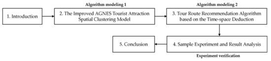
Figure 1. The research work and the structure of the paper.

2. The Improved AGNES Tourist Attraction Spatial Clustering Model

The features and spatial attributes of urban tourist attractions can vary widely. The feature attributes are the characteristics of one tourist attraction that differ from another one, such as tourist attraction classification, popularity, optimal traveling time, traveling fee, etc. The classification labels represent the characteristics or features of one tourist attraction, they determine the tourist attraction’s category, and they are typically mined from feature mapping data. The popularity is the average attraction capacity of one tourist attraction, which is determined from the online “big data” sources; for example, “Ctrip”, “Fliggy”, and “Qunar”, among others, provide popularity data for tourist attractions in China. The optimal traveling time and cost stand for the basic time and cost that are needed by the tourists to visit one tourist attraction. Each tourist attraction has various feature attributes that are associated to quantified values. The spatial attributes consider the geospatial location and positioning of a tourist attraction, including the discrete features and the indirectly correlated features. The discrete features should be considered independently for all tourist attractions [33]. Indirectly, the correlated features represent that each tourist attraction is connected with another one by urban roads and tourists can move between two tourist attractions freely. Tourist attraction attributes determine that tourist attractions have a close or distant relationship with each other, bringing different capacities for satisfying tourist interests. The precondition of selecting the tourist attractions to be visited is to confirm the classification that meet the tourist needs and interests. Therefore, the urban tourist attractions should be clustered primarily.

2.1. The Foundation of Tourist Attraction Attribute Label Matrix Model

The preconditions for the clustering algorithm confirmed the tourist attraction attributes and developed the association model that would measure the degree of correlation among the attractions. The degree of correlation among their attributes would be determined by their features as well as by their spatial factors. Thus, the clustering model should combine with the feature attribute factors and the spatial attribute factors [34].

The arbitrary typical tourist attraction in a tourism city is the tourist attraction element $s_{(i)}$, and it belongs to one certain tourist attraction classification. All the elements of $s_{(i)}$ form an entire research range, and it is the tourist attraction research domain $S$. The domain $S$ contains different types of tourist attractions, and it can be divided into several classifications.

The inner characteristics of one tourist attraction are the feature attributes, and they are noted as ${t_1}_{(i1)}$. The feature attributes influence tourist choices on the interest tendency and intelligent system’s search results of tourist attraction clusters and specific tourist attractions. The factor $i_1$ is the footnote of the feature attribute. Meanwhile, the tourist-attraction geolocation is the spatial attribute factor ${t_2}_{(i2)}$, and $i_2$ is the factor’s footnote. The tourist attraction attributes include $m$ number of feature attributes ${t_1}_{(i1)}$ and $n$ number of spatial attributes ${t_2}_{(i2)}$, $i_1\in (0,m]\subset {\mathrm{Z}}^{+}$, $i_2\in (0,n]\subset {\mathrm{Z}}^{+}$. Each factor ${t_1}_{(i1)}$ or ${t_2}_{(i2)}$ is one feature attribute label and spatial attribute label of $s_{(i)}$, and collectively, the tourist attraction attribute label.

The feature attribute ${t_1}_{(i1)}$ includes $u_{(i1)}$ items of classifying indices $t_{1(i1,j1)}$, $j_1\in (0,\alpha ]\subset {\mathrm{Z}}^{+}$, $j_1$ is the footnote of ${t_1}_{(i1,j1)}$, and $\alpha$ is the maximum number of ${t_1}_{(i1)}$. The $1\times u_{(i1)}$ dimension matrix ${t_1}_{(i1)}$ is formed by $u_{(i1)}$ items of $t_{1(i1,j1)}$ in the factor ${t_1}_{(i1)}$ and determines the No. ${t_1}_{(i1)}$ feature attribute and tourists’ interest tendency. The tourist attraction feature attribute label vector is ${t_1}_{(i1)}$. The spatial attribute ${t_2}_{(i2)}$ includes $u_{(i2)}$ items of classifying indices $t_{2(i2,j2)}$, $j_2\in (0,\alpha ]\subset {\mathrm{Z}}^{+}$, $j_2$ is the footnote of the indices $t_{2(i2,j2)}$ of ${t_2}_{(i2)}$, and $\alpha$ is the maximum number of ${t_2}_{(i2)}$. The $1\times u_{(i2)}$ dimension matrix ${t_2}_{(i2)}$ is formed by $u_{(i2)}$ items of $t_{2(i_2,j_2)}$ in the factor ${t_2}_{(i2)}$ and determines the No. ${t_2}_{(i2)}$ spatial attribute, and it is the spatial attribute label vector ${t_2}_{(i2)}$. The classifying index of the spatial attribute is formed to match the attribute label vector and create the attribute matrix. The vector’s rank meets $rank(t_{1(i1)})=u_{(i1)}$, and $rank({t_2}_{(i2)})=u_{(i2)}$.

For the tourist attraction attribute label matrix $T$, it is formed by $m$ number of ${t_1}_{(i1)}$ and $n$ number of ${t_2}_{(i2)}$ and determines the tourist attraction’s features and spatial attributes as well as influences the tourists’ interest tendency. The matrix $T$ meets the following conditions: The matrix row is the vector ${t_1}_{(i1)}$ or ${t_2}_{(i2)}$. The matrix column is the element of the vector ${t_1}_{(i1)}$ or ${t_2}_{(i2)}$. The matrix contains $m+n$ number of rows and $\alpha$ number of columns. The rows from 1 to $m$ relate to the vector $t_{1(i1)}~i_1\in (0,m]\subset {\mathrm{Z}}^{+}$, the $m+1$ to $m+n$ rows relate to the vector ${t_2}_{(i2)}~i_2\in (0,n]\subset {\mathrm{Z}}^{+}$. One tourist attraction relates to one matrix element distribution. Equation (1) is the general formula of the matrix $T$ and its element distribution.

$$T={\left[\begin{array}{cccccc}{t}_{1(1)},& \dots ,& t_{1(m)},& t_{2(1)},& \dots ,& t_{2(n)}\end{array}\right]}^T=\left[\begin{array}{cccccc}{t_1}_{(1,1)}& {t_1}_{(1,2)}& {t_1}_{(1,3)}& \dots & 0& 0\\ & & \dots & & \dots & \\ {t_1}_{(m,1)}& {t_1}_{(m,2)}& \dots & & \dots & {t_1}_{(m,\alpha )}\\ {t_2}_{(1,1)}& {t_2}_{(1,2)}& \dots & 0& \dots & {t_2}_{(1,\alpha )}\\ & & \dots & & & \\ {t_2}_{(m+n,1)}& {t_2}_{(m+n,2)}& \dots & {t_2}_{(m+n,4)}& \dots & 0\end{array}\right]$$

(1)

The feature attributes and spatial attributes are quantified. The feature attributes include tourist attraction classification ${t_1}_{(1)}$, popularity ${t_1}_{(2)}$, optimal travel time ${t_1}_{(3)}$, and traveling fee ${t_1}_{(4)}$. The spatial attribute mainly relates to the longitude and latitude coordinates $({t_2}_{(1)},{t_2}_{(2)})~(l,B)$ of the tourist attraction [35]. The feature attributes ${t_1}_{(i1)}$ and the spatial attributes ${t_2}_{(i2)}$ are quantified, where ${t_1}_{(1)}$ is tourist attraction classification; ${t_1}_{(2)}$ is popularity degree, noted as $h_o$, $h_o\in (0,1)\subset {\mathrm{R}}^{+}$, representing the users’ average evaluation scores on the website; ${t_1}_{(3)}$ is the optimal travel time, noted as $t_b$, unit: hour; and ${t_1}_{(4)}$ is the traveling fee (cost), noted as $c_o$, unit: CNY, ¥ yuan. The spatial attributes include longitude ${t_2}_{(1)}~l$ and latitude ${t_2}_{(2)}~B$. Each attribute factor includes a specific data value range which forms the tourist attraction feature attribute label vector ${t_1}_{(i1)}$ and spatial attribute label vector ${t_2}_{(i2)}$. The classification factor is determined by the tourist attraction’s inner attributes and it is the critical index to distinguish different tourist attractions and an important reference for a smart system to select a tourist attraction cluster and specific tourist attractions. The popularity degree represents the average preference of tourists on a tourist attraction $s_{(i)}$. The optimal travel time represents the most suitable time for tourists to visit a tourist attraction $s_{(i)}$. The traveling fee represents the minimum cost for tourists to visit a tourist attraction $s_{(i)}$ such as the fee for the entrance ticket. The formed tourist attraction attribute label matrix $T$ is ${[{{\mathbf{t}}_1}_{(1)},\dots {{\mathbf{t}}_1}_{(m)}, {{\mathbf{t}}_2}_{(1)},\dots {{\mathbf{t}}_2}_{(n)}]}^T$, each label vector includes the specific index $t_{1(i1,j1)}$ or $t_{2(i_2,j_2)}$. Quantify the index $t_{1(i1,j1)}$ or $t_{2(i_2,j_2)}$ as follows, in which the classification factor is also quantified into a specific value.

$T$:{${t_1}_{(1)}$: Tourist attraction classification; ${t_1}_{(2)}$: popularity degree; ${t_1}_{(3)}$: the optimal travel time; ${t_1}_{(4)}$: traveling fee; ${t_2}_{(1)}$: longitude; ${t_2}_{(2)}$: latitude};

$t_{1(1)}$: {${t_1}_{(1,1)}$: nature park (1.00); ${t_1}_{(1,2)}$: humanistic history (2.00); ${t_1}_{(1,3)}$: amusement park (3.00); ${t_1}_{(1,4)}$: leisure shopping (4.00); ${t_1}_{(1,5)}$: modern science and technology (5.00); ${t_1}_{(1,6)}$: artistic aesthetics (6.00)};

$t_{1(2)}$:{${t_1}_{(2,1)}$: $h_o\in (0,0.25]$; ${t_1}_{(2,2)}$: $h_o\in (0.25,0.50]$; ${t_1}_{(2,3)}$: $h_o\in (0.50,0.75]$; ${t_1}_{(2,4)}$: $h_o\in (0.75,1.00)$}, ${t_1}_{(2,j_1)}\in {\mathrm{R}}^{+}$;

$t_{1(3)}$:{${t_1}_{(3,1)}$: $t_b\in (0,2.0]$: ${t_1}_{(3,2)}$: $t_b\in (2.0,4.0]$; ${t_1}_{(3,3)}$: $t_b\in (4.0,6.0]$; ${t_1}_{(3,4)}$: $t_b\in (6.0,+\infty )$}, ${t_1}_{(3,j_1)}\in {\mathrm{R}}^{+}$;

$t_{1(4)}$:{${t_1}_{(4,1)}$: $c_o\in (0,100]$; ${t_1}_{(4,2)}$: $c_o\in (100,200]$; ${t_1}_{(4,3)}$: $c_o\in (200,300]$; ${t_1}_{(4,4)}$: $c_o\in (300,+\infty )$}, ${t_1}_{(3,j_1)}\in {\mathrm{R}}^{+}$.

When all the feature attribute label vectors ${t_1}_{(i1)}$ for all the elements $s_{(i)}$ in domain $S$ are confirmed, the correction parameter for each vector ${t_1}_{(i1)}$ is then defined to normalize all the values.

The impact of each feature attribute label vector impact on calculating the degree of correlation between the tourist attractions should be in the same order of magnitude, and thus the feature attribute label vector normalized parameter ${{\delta }_1}_{(i1)}$ is generated, and all the labels are normalized according to a range of $(0,1]$. According to the range of the vector ${t_1}_{(i1)}$, each normalized parameter ${{\delta }_1}_{(i1)}$ is confirmed as follows:

$${{\delta }_1}_{(1)}=0.100,{{\delta }_1}_{(2)}=1.000,{{\delta }_1}_{(3)}=0.100,{{\delta }_1}_{(4)}=0.001.$$

The parameter ${{\delta }_1}_{(i1)}$ is used to normalize each vector ${t_1}_{(i1)}$ in the matrix $T$ to obtain a new normalized matrix $T_{\delta }$. As compared to the matrix $T$, the elements in the matrix $T_{\delta }$ are all normalized except for the vector ${t_2}_{(i2)}$. Equation (2) is the general formula for the matrix $T_{\delta }$.

$$\left\{\begin{array}{l}{T}_{\delta }={\left[\begin{array}{cccccc}{{\delta }_1}_{(1)}\cdot {t_1}_{(1)},& \dots ,& {{\delta }_1}_{(m)}\cdot t_{1(m)},& t_{2(1)},& \dots ,& t_{2(n)}\end{array}\right]}^T\\ T_{\delta }=\left[\begin{array}{cccccc}{{\delta }_1}_{(1)}\cdot {t_1}_{(1,1)}& {{\delta }_1}_{(2)}\cdot {t_1}_{(1,2)}& {{\delta }_1}_{(3)}\cdot {t_1}_{(1,3)}& \dots & 0& 0\\ & & \dots & & \dots & \\ {{\delta }_1}_{(m)}\cdot {t_1}_{(m,1)}& {{\delta }_1}_{(m)}\cdot {t_1}_{(m,2)}& \dots & & \dots & {{\delta }_1}_{(m)}\cdot {t_1}_{(m,\alpha )}\\ {t_2}_{(1,1)}& {t_2}_{(1,2)}& \dots & 0& \dots & {t_2}_{(1,\alpha )}\\ & & \dots & & & \\ {t_2}_{(m+n,1)}& {t_2}_{(m+n,2)}& \dots & {t_2}_{(m+n,4)}& \dots & 0\end{array}\right]\end{array}\right.$$

(2)

Based on the tourist attraction attribute label matrix $T$ and the normalized matrix $T_{\delta }$, the tourist attraction research domain $S$ clustering algorithm is created.

2.2. The Tourist Attraction Domain Clustering Algorithm Based on the Improved AGNES Algorithm

The aim of the tourist attraction domain clustering was to obtain a cluster with a high degree of correlation among the attributes, realizing that the tourist attractions in the same clusters have a high degree of correlation among the attributes while those in different clusters have a low degree of correlation among the attributes, and finally to guide the smart system into precisely matching tourist interests. The clustering process was the automatic process driven by data, and the clustering criteria could differentiate according to the different clustering targets. When a spatial dot is the only a location point in a coordinate system, a traditional clustering algorithm will assume the spatial distance as a singular criterion. Tourist attractions have spatial attributes and feature attributes, and thus the criteria for tourist-attraction clustering should combine both factors.

The $k$ number of elements $s_{(i)}$ in the domain $S$ are clustered by the clustering algorithm, and the tourist attractions $s_{(i)}$, which have a high degree of correlation among the attributes and are in the same cluster $S_{(i)}$, while the tourist attractions $s_{(i)}$ and ${}^{\neg }{s}_{(i)}$, which have a low degree of correlation among the attributes, are in the different clusters $S_{(i)}$ and ${}^{\neg }{S}_{(i)}$, $k\in \mathrm{N}$. The cluster’s element is noted as $s_{(i,j)}$, $i$ is the footnote of the cluster $S_{(i)}$, $j$ is the footnote of the element in the cluster $S_{(i)}$. In all, it is supposed that the clustering algorithm forms $p$ number of clusters, $p\in \mathrm{N}$ and $p<<k$. Assume that the cluster $S_{(i)}$ contains $k_{(i)}$ number of elements $s_{(i,j)}$, and $j\in (0,k_{(i)}]\subset {\mathrm{Z}}^{+}$, so thus ${\displaystyle {\sum }_{i=1}^p{k}_{(i)}}=k$. The elements $s_{(i,j)}$ in the same cluster $S_{(i)}$ have a high degree of correlation among the attributes, and elements $s_{(i,j)}$ in different clusters $S_{(i)}$ and ${}^{\neg }{S}_{(i)}$ have a low degree of correlation among the attributes. An arbitrary cluster $\forall S_{(i)}$ contains at least one element $s_{(i)}$. Arbitrary one element $\forall s_{(i)}$ in the domain $S$ only belongs to one certain cluster $S_{(i)}$. Clusters $S_{(i)}$ and other cluster ${}^{\neg }{S}_{(i)}$ have no intersection, but in the aspect of spatial analysis, the clusters may have a buffer overlap in the city space. The union of all the clusters $S_{(i)}$ is the domain $S$, and $i\in (0,p]\subset \mathrm{N}$. In the domain $S$, there are at least two clusters, that is $p\ge 2$.

Whether the tourist attraction element $s_{(i)}$ should be absorbed into the cluster $S_{(i)}$ is determined by the objective function ${\xi }_{(s_{(i1)},s_{(i2)})}$ among $s_{(i)}$ and other tourist attractions. The function is determined by several clustering factors, including the feature attribute factors ${t_1}_{(i1)}$ and the spatial attributes factors ${t_2}_{(i2)}$. As to the two independent tourist attractions $s_{(i1)}$ and $s_{(i2)}$, their degree of correlation includes their geospatial relationship and the spatial attributes correlation, and thus their neighborhood relationship is determined by consensus of the two factors. Therefore, the matrix $T$ and matrix $T_{\delta }$ both contain the factors classification ${t_1}_{(1)}$, popularity degree ${t_1}_{(2)}$, the optimal travel time ${t_1}_{(3)}$, and the traveling cost ${t_1}_{(4)}$, as well as longitude and latitude $({t_2}_{(1)},{t_2}_{(2)})~(l,B)$. The improved Minkowski distance is applied to for the objective function, and the clustering criteria should consider features and spatial attributes simultaneously. The pseudo-code of the process to create the function ${\xi }_{(s_{(i1)},s_{(i2)})}$. (Algorithm 1) is shown as follows.

Algorithm 1: The process to create the function ${\xi }_{(s_{(i1)},s_{(i2)})}$
1:	Step 1: Confirm $T_{\delta (i)}$ for $s_{(i)}$ in $S$.
2:	Step 2: For the $s_{(i1)}$, extract the non-zero elements ${{\delta }_{1,1}}_{(i1)}\cdot {t_{1,1}}_{(i1,j1)}$ and ${t_{2,1}}_{(i2,j2)}$ in   ${{\delta }_{1,1}}_{(i1)}\cdot {t_{1,1}}_{(i1)}$ and ${t_{2,1}}_{(i2)}$ of ${T_{\delta }}_{(i1)}$. Transpose ${T_{\delta }}_{(i1)}$ to ${{T_{\delta }}_{(i1)}}^T$.
3:	Step 3: For the $s_{(i2)}$, extract the non-zero elements ${{\delta }_{1,2}}_{(i1)}\cdot {t_{1,2}}_{(i1,j1)}$ and ${t_{2,2}}_{(i2,j2)}$ in   ${{\delta }_{1,1}}_{(i1)}\cdot {t_{1,1}}_{(i1)}$ and ${t_{2,1}}_{(i2)}$ of $T_{\delta (i2)}$. Transpose ${T_{\delta }}_{(i2)}$ to ${{T_{\delta }}_{(i2)}}^T$.
4:	Step 4: Confirm the Minkowski distance $d(x,y)$ as the objective function ${\xi }_{(s_{(i1)},s_{(i2)})}$

The Minkowski distance between the two samples $x$ and $y$ is shown in Equation (3). The Minkowski distance is used to define the objective function ${\xi }_{(s_{(i1)},s_{(i2)})}$, shown as Equations (4) and (5). According to the function ${\xi }_{(s_{(i1)},s_{(i2)})}$, the norm value of the function is used to judge whether the tourist attractions $s_{(i1)}$ and $s_{(i2)}$ belong to the same cluster. Therefore, the function ${\xi }_{(s_{(i1)},s_{(i2)})}$ value is set as the clustering criterion.

$$d(x,y)=‖x-y‖p={[{{\displaystyle {\sum }_{i=1}^n|x_{(i)}-y_{(i)}|}}^r]}^{1/r}$$

(3)

$${\xi }_{(s_{(i1)},s_{(i2)})}={‖{T_{\delta (i1)}}^T-{T_{\delta (i2)}}^T‖}_2$$

(4)

$${\xi }_{(s_{(i1)},s_{(i2)})}={[{{\displaystyle {\sum }_{i1=1}^m|{{\delta }_{1,1}}_{(i1)}\cdot {t_{1,1}}_{(i1,j1)}-{{\delta }_{1,2}}_{(i1)}\cdot {t_{1,2}}_{(i1,j1)}|}}^2+{{\displaystyle {\sum }_{i2=1}^n|{t_{2,1}}_{(i2,j2)}-{t_{2,2}}_{(i2,j2)}|}}^2]}^{1/2}$$

(5)

In the process of generating clusters, the $k$ number of elements $s_{(i)}$ are dynamically stored into one matrix $K^{\wedge }(p\times \max k_{(i)})$ in the cluster code sequence by the clustering algorithm. Each row in the matrix dynamically stores the related cluster’s elements. When the clustering algorithm ends, all the tourist attraction elements are consistently stored in the matrix $K(p\times \max k_{(i)})$ according to the cluster code $i$ and cluster’s element code $j$. The matrix row number is $p$, the column number is $\max k_{(i)}$, in which $k$ number of elements are used to store tourist attractions, while the other $p\times \max k_{(i)}-k$ number of elements are stored as 0. The row rank meets at $rank({K^{\wedge }}_{(p•)})\le p$ and $rank(K_{(p•)})\le p$. The column rank meets at $rank({K^{\wedge }}_{(•\max k_{(i)})})\le \max k_{(i)})$ and $rank(K_{(•\max k_{(i)})})\le \max k_{(i)})$. The matrix $K(p\times \max k_{(i)}))$ has at least two non-empty rows. Equations (6) and (7) relate to the matrix $K^{\wedge }(p\times \max k_{(i)})$ and $K(p\times \max k_{(i)})$, in the formula, ${s_{(i)}}^{\wedge }$ represents the element with random storage value.

$$K^{\wedge }(p\times \max k_{(i)}))=\left[\begin{array}{ccccc}{s_{(1)}}^{\wedge }& {s_{(2)}}^{\wedge }& \dots & 0& {s_{(i1)}}^{\wedge }\\ {s_{(i1+1)}}^{\wedge }& \dots & 0& \dots & {s_{(i2)}}^{\wedge }\\ 0& \dots & {s_{(i)}}^{\wedge }& \dots & 0\\ {s_{(i3)}}^{\wedge }& \dots & 0& \dots & {s_{(k)}}^{\wedge }\end{array}\right]$$

(6)

$$K(p\times \max k_{(i)}))=\left[\begin{array}{ccccc}{s}_{(1,1)}& s_{(1,2)}& \dots & \dots & s_{(1,\max k(1))}\\ s_{(2,1)}& \dots & s_{(2,k(2))}& \dots & s_{(2,\max k(2))}\\ \dots & \dots & s_{(i,j)}& \dots & 0\\ s_{(p,1)}& \dots & 0& s_{(p,\max k(p))}& 0\end{array}\right]$$

(7)

The tourist attraction clustering objective function ${\xi }_{(s_{(i1)},s_{(i2)})}$ is set as the improved AGNES clustering algorithm criterion. The $k$ number of elements $s_{(i)}$ in the domain $S$ are clustered into $p$ number of clusters and stored into the matrix $K(p\times \max k_{(i)}))$.

In the improved AGNES clustering algorithm, in a single instance of dot gathering from the bottom to top, a seed point element $s_{(i)}*$ is chosen as the tourist attraction representing a certain cluster $S_{(i)}$. Take the element $s_{(i)}*$ as a criterion to calculate and judge the objective function ${\xi }_{(s_{(i1)},s_{(i2)})}$ to confirm another element to be gathered and form the cluster. The tourist attractions that are not the seed point are noted as ${}^{\neg }{s}_{(i)}*$.

In one instance of gathering from bottom to top, if one point ${}^{\neg }{s}_{(i)}*$ belongs to the cluster $S_{(i)}$, the point ${}^{\neg }{s}_{(i)}*$ is absorbed into the cluster $S_{(i)}$, the edge $l(s_{(i)}{,}^{\neg }{s}_{(i)})$ connecting $s_{(i)}*$ and ${}^{\neg }{s}_{(i)}*$ is generated. When the clustering algorithm ends, the $k_{(i)}$ number of tourist attractions as well as the gathered $k(i)-1$ number of topological edges $l(s_{(i)}{,}^{\neg }{s}_{(i)})$ in the cluster $S_{(i)}$ form a cluster structure tree ${T_r}_{(S_{(i)})}$. The spatial range that is expanded by the tree ${T_r}_{(S_{(i)})}$ forms the cluster spatial buffer ${r_a}_{(S_{(i)})}$. The edge $l(s_{(i)}{,}^{\neg }{s}_{(i)})$ and the tree ${T_r}_{(S_{(i)})}$ show the visualized process of the improved AGNES algorithm. The buffer ${r_a}_{(S_{(i)})}$ is the visualized range for each cluster. Since the objective function ${\xi }_{(s_{(i1)},s_{(i2)})}$ contains both feature attributes and spatial attributes, different buffers ${r_a}_{(S_{(i)})}$ may intersect. Figure 2 shows the spatial relationship among the cluster $S_{(i)}$ topological edge $l(s_{(i)}{,}^{\neg }{s}_{(i)})$, cluster structure tree ${T_r}_{(S_{(i)})}$, and the cluster spatial buffer ${r_a}_{(S_{(i)})}$. Figure 2a is an edge $l(s_{(i)}{,}^{\neg }{s}_{(i)})$, Figure 2b is the tree ${T_r}_{(S_{(i)})}$ which is formed by several edges $l(s_{(i)}{,}^{\neg }{s}_{(i)})$, and Figure 2c is the buffer ${r_a}_{(S_{(i)})}$ which is formed by the cluster structure tree ${T_r}_{(S_{(i)})}$.

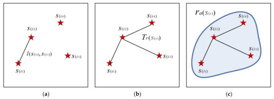
Figure 2. The spatial relationship among the cluster $S_{(i)}$ topological edge $l(s_{(i)}{,}^{\neg }{s}_{(i)})$, cluster structure tree ${T_r}_{(S_{(i)})}$, and the cluster spatial buffer ${r_a}_{(S_{(i)})}$. (a) is an edge $l(s_{(i)}{,}^{\neg }{s}_{(i)})$, (b) is the tree ${T_r}_{(S_{(i)})}$ that is formed by several edges $l(s_{(i)}{,}^{\neg }{s}_{(i)})$, and (c) is the buffer ${r_a}_{(S_{(i)})}$ that is formed by the cluster structure tree ${T_r}_{(S_{(i)})}$.

According to the modeling principle, the improved AGNES clustering algorithm has been created. The smart system will search the optimal tourist attractions and tour routes by the $p$ number of clusters and tourists’ interests, time budget, and cost budget, etc. The pseudo-code of the process to create the improved AGNES clustering algorithm (Algorithm 2) is shown as follows:

Algorithm 2: The process to create the improved AGNES clustering algorithm
1:	Step 1: Create $\xi (s_{(i1)},s_{(i2)})$ to store $S_{to}(•)$ and its descending $S_{to}{(•)}^d$ with element    $S_{\mathrm{to}(i,j)}$. The value $\xi (s_{(i1)},s_{(i2)})$ is stored in the descending order from the    first row first column to the last one.
2:	Step 2: Confirm seed point $s_{(i)}*$.   Sub-step 1: Take the former $e$ number of elements of the matrix $S_{to}{(•)}^d$.   Sub-step 2: Note ${S_{\mathrm{to}(\max i,\max j)}}^d$ relates to the tourist attractions $a_{(2e-1)}$ and $a_{(2e)}$.   Sub-step 3: $a_{(o)}$ relates to the noted $s_{(i)}$ in $S$.   Sub-step 4: Search ${S_{\mathrm{to}(i,j)}}^d$ on $\forall s_{(i1)}$ and $\forall s_{(i2)}$ of $\forall a_{(o1)}$ and $\forall a_{(o2)}$ in $S_{to}{(•)}^d$.   Sub-step 5: The p number of $a_{(i)}$ with the maximum value ${S_{\mathrm{to}(i,j)}}^d$ as $s_{(i)}*$.
3:	Step 3: Form the cluster $S_{(i)}$ by $s_{(i)}*$.   Sub-step 1: Store the No.1 $s_{(i)}*$ into ${K^{\wedge }}_{(i,1)}$ in $K^{\wedge }$.   Sub-step 2: Search $\xi (s_{(i)}*{,}^{\neg }{s}_{(i)}*)$ and find $\min \xi (s_{(i)}*{,}^{\neg }{s}_{(i)}*)$.   Sub-step 3: Judge ${}^{\neg }{s}_{(i)}*$ whether belongs to $s_{(i)}$ cluster $S_{(i)}$.   If ${}^{\neg }{s}_{(i)}*$ belongs to $S_{(i)}$, store it into the $S_{(i)}$ row; If it does not belong,    store into another row.   Sub-step 4: Form $l{(}^{\neg }{s}_{(i)}*,s_{(i)}*)$ with the $s_{(i)}*$ and its cluster $S_{(i)}$ tourist attractions.
4:	Step 4: For the structure tree $T_{r(S_{(i)})}$.
5:	Step 5: Expand the tree $T_{r(S_{(i)})}$ from $l{(}^{\neg }{s}_{(i)}*,s_{(i)}*)$ with a radius range $r$ and form   the cluster spatial buffer $r_{a(S_{(i)})}$.

The proposed AGNES clustering algorithm is significantly different from those that have been used in previous research (see the Introduction section). First, the aim is totally different; the proposed method is to find out the classifications of city tourist attractions, and it tends to extract the correlation among different tourist attractions and calculate the degree of correlation between two tourist attractions, and finally output the tourist attraction clusters. This clustering process is the critical step for tourists’ interests matching the tourist attractions’ attributes. The previous methods did not concern tourist attractions clustering, and they mainly tended to find out the tourists’ clusters, tourists’ behaviour, and the relationship between the collaborative economy and tourism, etc. Second, the parameters that were used in developing the AGNES model are different. Besides the spatial attributes, the proposed AGNES algorithm makes improvements on the clustering criterion function by adding tourist attraction’s feature attributes, which makes the tourist attraction clustering more logical, since the clusters and tourist attractions are grouped to match the tourists’ interests. The previous methods directly used the AGNES algorithm itself on the basis of spatial attributes such as longitude and latitude. Third, since the proposed AGNES algorithm is an improved method, the detailed steps on modeling the algorithm are provided in the paper. It is an important research content and precondition of the whole research work. In previous studies, the AGNES algorithm is merely a tool that is used by the authors without detailed algorithm modeling process.

3. Tour-Route-Recommendation Algorithm Based on the Space-Time Deduction

The selection of tourist attractions and tour-route design are the two critical factors for any tour itinerary. Tourists must choose the tourist attractions that best match their interests and then plan the most reasonable route based on their selections. Time and cost are always limitations, to which travel and participation significantly contribute. Therefore, with available time and financial expectations as fixed conditions, a “smart” system should be able to recommend attractions that best-match an individual’s preferences as well as optimize the transportation route. Since the mode of transportation would be largely influenced by the tourist themselves, it was a crucial factor for consideration when developing our model [36,37].

3.1. Tourist Attraction Reachability Space Model Based on Interest Matrix and Geographical Position

The precondition for the smart system to recommend tourists with tour routes was obtaining the tourist interest data. The interest data were set as the input labels and then matched with the tourist attraction attributes. The capacity of each tourist attraction to satisfy a tourist’s interests would be different, and this capacity was defined as the reachable capacity, the value of which would dictate the likelihood of its recommendation by the system. Therefore, creating a reachability space model between the tourist interest data and the tourist attractions was the precondition when searching for tourist attractions that would best satisfy an individual’s interests [38,39].

The tourist interest label vector ${n_1}_{(i1)}$ and spatial positioning vector ${n_2}_{(i2)}$ have the same dimension as the vectors of ${t_1}_{(i1)}$ and ${t_2}_{(i2)}$, and they represent the tourist-interest data. The variable ${n_1}_{(i1)}$ is a $1\times u_{(i1)}$ dimension vector. The interest label factor ${n_1}_{(i1)}$ contains $u_{(i1)}$ items of different classifying indices ${n_1}_{(i1,j1)}$ and $j_1\in (0,\alpha ]\subset {\mathrm{Z}}^{+}$. The variable $j_1$ is the footnote for the index ${n_1}_{(i1,j1)}$ of the factor ${n_1}_{(i1)}$, and $\alpha$ is the maximum number of the index. The variable ${n_2}_{(i2)}$ is a $1\times u_{(i2)}$ dimension vector. The spatial positioning factor ${n_2}_{(i2)}$ contains $u_{(i2)}$ items of different classifying indices ${n_2}_{(i_2,j_2)}$ and $j_2\in (0,\alpha ]\subset {\mathrm{Z}}^{+}$, where $j_2$ is the footnote for the index ${n_2}_{(i_2,j_2)}$ of the factor ${n_2}_{(i2)}$, and $\alpha$ is the maximum number of the index. The number of vectors ${n_1}_{(i1)}$ and ${n_2}_{(i2)}$ are $m$ and $n$.

The starting point of one tour route for the tourist is $S_t$. The point $S_t$ determines the dimension and specific values of the spatial location vector ${n_2}_{(i2)}$. The matrix $N$ is formed by $m$ number of feature attribute label vectors ${n_1}_{(i_1)}$ and $n$ number of spatial attribute label vector ${n_2}_{(i2)}$ and represents the tourists’ interest tendency. The matrix row is the vector ${n_1}_{(i_1)}$ or ${n_2}_{(i2)}$ and the column is the specific element of the vector ${n_1}_{(i_1)}$ or ${n_2}_{(i2)}$. It contains $m+n$ number of rows and $\alpha$ number of columns. The No.1 to No.$m$ rows relate to the vector ${n_1}_{(i_1)}~i_1\in (0,m]\subset {\mathrm{Z}}^{+}$, the No.$m+1$ to No.$m+n$ rows relate to the vector ${n_2}_{(i2)}~i_2\in (0,n]\subset {\mathrm{Z}}^{+}$. When the tourist interest data are confirmed, the arbitrary row ${n_1}_{(i_1)}$ will form one item of an attribute element value ${n_1}_{(i_1,j_1)}$, $j_1\in (0,\alpha ]\subset {\mathrm{Z}}^{+}$, and the other elements are 0. The Equation (8) is the general formula $N$ and its specific elements.

$$N={\left[\begin{array}{cccccc}{n}_{1(1),}& \dots ,& n_{1(m)},& n_{2(1)},& \dots ,& n_{2(n)}\end{array}\right]}^T=\left[\begin{array}{cccccc}{n_1}_{(1,1)}& {n_1}_{(1,2)}& {n_1}_{(1,3)}& \dots & 0& 0\\ & & \dots & & \dots & \\ {n_1}_{(m,1)}& {n_1}_{(m,2)}& \dots & & \dots & {n_1}_{(m,\alpha )}\\ {n_2}_{(1,1)}& {n_2}_{(1,2)}& \dots & 0& \dots & {n_2}_{(1,\alpha )}\\ & & \dots & & & \\ {n_2}_{(m+n,1)}& {n_2}_{(m+n,2)}& \dots & {n_2}_{(m+n,4)}& \dots & 0\end{array}\right]$$

(8)

The matrix $N$ elements are related to the matrix $T$ elements, including tourist classification ${n_1}_{(1)}$, popularity degree ${n_1}_{(2)}$, travel time ${n_1}_{(3)}$, traveling fee ${n_1}_{(4)}$, longitude ${n_2}_{(1)}$, and latitude ${n_2}_{(2)}$.

${n_1}_{(1)}$:{${n_1}_{(1,1)}$: nature park (1.00); ${n_1}_{(1,2)}$: humanistic history (2.00); ${n_1}_{(1,3)}$: amusement park (3.00); ${n_1}_{(1,4)}$: leisure shopping (4.00); ${n_1}_{(1,5)}$: modern science and technology (5.00); ${n_1}_{(1,6)}$: artistic aesthetics (6.00).};

${n_1}_{(2)}$:{${n_1}_{(2,1)}$: $h_o\in (0,0.25]$; ${n_1}_{(2,2)}$: $h_o\in (0.25,0.50]$; ${n_1}_{(2,3)}$: $h_o\in (0.50,0.75]$; ${n_1}_{(2,4)}$: $h_o\in (0.75,1.00)$}, ${n_1}_{(2,j_1)}\in {\mathrm{R}}^{+}$;

${n_1}_{(3)}$:{${n_1}_{(3,1)}$: $t_b\in (0,2.0]$; ${n_1}_{(3,2)}$: $t_b\in (2.0,4.0]$; ${n_1}_{(3,3)}$: $t_b\in (4.0,6.0]$; ${n_1}_{(3,4)}$: $t_b\in (6.0,+\infty )$}, ${n_1}_{(3,j_1)}\in {\mathrm{R}}^{+}$;

${n_1}_{(4)}$:{${n_1}_{(4,1)}$: $c_o\in (0,100]$; ${n_1}_{(4,2)}$: $c_o\in (100,200]$; ${n_1}_{(4,3)}$: $c_o\in (200,300]$; ${n_1}_{(4,4)}$:$c_o\in (300,+\infty )$}, ${n_1}_{(3,j_1)}\in {\mathrm{R}}^{+}$.

The spatial location vector ${n_2}_{(i2)}$ of the matrix $N$ is determined by the longitude and latitude of the point $S_t$.

The correlation between the tourists’ interest and the tourist attraction attributes is determined by the interest quantitative matching objective function ${\xi }_{(N,T)}$. Transfer the feature attribute label vector normalized parameter ${{\delta }_1}_{(i_1)}$ and take it as the parameter to create the function ${\xi }_{(N,T)}$, then confirm the tourist-interest data. Traverse $j_1,j_2~(0,\alpha ]$, search and extract the non-zero elements ${{\delta }_1}_{(i_1)}\cdot {n_1}_{(i_1,j_1)}$ and ${n_2}_{(i_2,j_2)}$ in the matrix $N$ label vector ${{\delta }_1}_{(i_1)}\cdot {n_1}_{(i_1)}$ and ${n_2}_{(i2)}$. Transpose the matrix $N$ and generate the matrix $N^T$. Create the norm relationship of the Minkowski distance between the tourists’ interests and the tourist attractions, shown in the Equations (9) and (10). Calculate the function ${\xi }_{(N,T)}$ between the matrix $N$ and the matrix $T$. Use the interest quantitative matching objective function matrix $P_{\xi (N,T)}$ to store the function value.

$${{\xi }_{(N,T)}=‖N^T-T^T‖}_2$$

(9)

$${\xi }_{(N,T)}={[{{\displaystyle {\sum }_{i1=1}^m|{{\delta }_1}_{(i1)}\cdot {n_1}_{(i1,j1)}-{{\delta }_1}_{(i_1)}\cdot {t_1}_{(i1,j1)}|}}^2+{{\displaystyle {\sum }_{i2=1}^n|{n_2}_{(i2,j2})-{t_2}_{(i2,j)}|}}^2]}^{1/2}$$

(10)

When the interest data remains the same, the tourist attractions $s_{(i)}$ in different clusters will generate different function values ${\xi }_{(N,T)}$. The values ${\xi }_{(N,T)}$ are stored in the sequence of the cluster $S_{(i)}$ footnote of the matrix $P_{\xi (N,T)}$. The value ${\xi }_{(N,T)}$ is stored in the $P_{\xi (N,T)}$ in ascending order from the first row and column to the last one. When tourists confirm the interest data, they contain the longitude and latitude of the starting point $S_t$. Taking the point $S_t$ as the center core, each row of the matrix $P_{\xi (N,T)}$ represents the correlation between the tourist attractions and the interest data, and also represents the reachability extent of the tourist attractions.

3.2. The Dynamic Space-Time Deduction Algorithm Based on the Travel Time and Cost

During a city tour, tourists expect to visit several tourist attractions in one day; tourists have different interests and levels of desire to visit various kinds of tourist attractions that will each involve different time investments and associated costs. Therefore, when the time and cost are fixed, the number of tourist attractions to be visited must be finite. According to the tourist attraction reachability model, the smart system would formulate a tour route that would best match tourist interests while meeting the time and cost conditions. Furthermore, depending on the mode of transportation that was chosen, the goal of saving time and cost could result in better attraction recommendations and optimized route-planning. Since travel time would be directly affected by the mode of transportation and route between attractions, the precondition for the dynamic space–time deduction of the tour-route-recommendation algorithm had the lowest path-searching cost [37,38].

3.2.1. The Shortest-Path-Searching Algorithm Based on the Space-Vector Lattice

After visiting a tourist attraction, tourists will move to the next one. This activity is based on specific activities. First, tourists will use a transportation mode such as walking, cycling, taxi service, etc. Second, they will travel city roads to the destination. Third, the moving process will consume time and cost.

The traffic space between two tourist attractions is the tourist attraction traffic subspace $\Phi$. The space $\Phi$ is the interval from point A to point B, and it is a vector space with coordinates, shown in Figure 3. The left bottom dot of the square $\Phi$ is the origin of coordinate. Each line represents an abstract city road. The line intersection $a_{(i)}$ represents the road intersection. In the Figure 3, the space $\Phi$ contains all city roads between the two points A and B. The road distance $d_{is}(a_{(i)},a_{(j)})$ of the edges CD, DE, EF, and CF in the small square CDEF may be different.

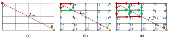
Figure 3. The space-vector lattice between the point A and B to search the shortest path. (a) is the spatial connecting line of the space $\Phi$. (b) is the spatial road and lattice relationship as well as the searching process for the series contained in the square $S_{qu}(A,a_{(1)},a_{(5)},a_{(6)})$. (c) is the spatial road-lattice relationship as well as the searching process for the series that is contained in the square $S_{qu}(A,a_{(2)},a_{(10)},a_{(12)})$.

Starting from the point A, search the path along the road until the point B is reached; in the whole process, all the searched points are listed in the spatial searching series $S_{eq}$. The searching series $S_{eq}$ represents a reachable path that is related to a searched distance $d_{is}(S_{eq})$. Figure 3 shows the shortest-path algorithm searching process.

The pseudo-code of the process to create the shortest-path algorithm (Algorithm 3) is shown as follows. This searching mode considers all the city roads and intersections between two points and finds the global minimum value, which may be more precise than the other shortest-path algorithms. The shortest path may reduce time and costs and thus increase the number of tourist attractions to be visited.

Algorithm 3:The process to create the shortest-path algorithm
1:	Step 1: Make line $l_{(AB)}$ between A and B in Figure 3a.
2:	Step 2: Take the points $a_{(6)}$, $a_{(12)}$, $a_{(18)}$
3:	Step 3: Search and compare $S_{eq}$ in $S_{qu}(A,a_{(1)},a_{(5)},a_{(6)})$ in Figure 3b.   Sub-step 1: Search $S_{eq}(A,a_{(1)},a_{(6)})$, noted as $S_{eq(1)}$, road distance is $d_{is}(S_{eq}(A,a_{(1)},a_{(6)}))$.   Sub-step 2: Search $S_{eq}(A,a_{(5)},a_{(6)})$, noted as $S_{eq(2)}$, road distance is $d_{is}(Seq(A,a_{(5)},a_{(6)})))$.   Sub-step 3: Find the minimum one $\min d_{is}{(S_{eq})}_{(1)}$ between A and $a_{(6)})$.
4:	Step 4: Search and compare $S_{eq}$ in $S_{qu}(A,a_{(2)},a_{(10)},a_{(12)})$ in Figure 3c.   Sub-step 1: Search $S_{eq}{(S_{eq}}_{(1)},a_{(7)},a_{(12)})$, $S_{eq}(S_{eq(1)},a_{(11)},a_{(12)})$, $S_{eq}(A,a_{(1)},a_{(2)}),a_{(7)},a_{(12)})$, $S_{eq}{(S_{eq}}_{(2)},a_{(11)},a_{(12)})$, $S_{eq}(Seq(2),a_{(7)},a_{(12)})$, $S_{eq}(A,a_{(5)},a_{(10)},a_{(11)},a_{(12)})$.   Sub-step 2: Find the minimum one $\min d_{is}{(S_{eq})}_{(2)}$ between A and $a_{(12)}$.
5:	Step 5: Continue searching until the square $S_{qu}(A,a_{(4)},a_{(20)},B)$ is finished. Find the minimum one $\min d_{is}{(S_{eq})}_{(4)}$ between A and B.

3.2.2. The Dynamic Space-Time Deduction Tour-Route-Searching Algorithm

Once the tourist attractions are been identified based on tourist interests, the travel time and cost would determine the number of tourist attractions to be visited and the optimal travel route, all of which would influence a tourist’s overall experience. Based on the matrix $P_{\xi (N,T)}$ and fixed time and cost conditions, the dynamic space-time deduction tour-route-searching algorithm was created. The basic process of the algorithm was as follows: using a daytrip as an example, a tourist confirms the travel time budget $t$ (unit: hour), traveling fee $c$ (unit: CNY ¥ yuan), and then chooses one transportation mode. Starting from the point $S_t$, search the shortest path between the point $S_t$ and tourist attractions and confirm the travel time using the chosen transportation mode. Iterate the visiting time in the tourist attractions and calculate the travel costs and any entrance or activity fees. Search the minimum time and cost between the point $St$ as well as all the tourist attractions and set the related point as the first tourist attraction $K_{(1)}$ to be visited. Starting from the $K_{(1)}$ point, search the next minimum travel time and cost tourist attraction $K_{(2)}$ until the total travel time or cost reaches the preset time budget $t$ or cost budget $c$, and then the optimal tour route is defined.

In a tour, the road interval from the point A to B is a cost iteration sub-unit $Q_{(i)}$. This sub-unit is the basic unit for the dynamic deduction process. The sum of the travel time contains the visiting time of a tourist attraction and the travel time from the point A to B; it is the time consumption $t_{(i)}$ of the sub-unit. The time $t_{(i)}$ is determined by the tourist attraction B visiting time and the travel time to the B. The sum of traveling costs contains the visiting fees of the tourist attractions and the travel costs from the point A to B; it is the cost consumption $c_{(i)}$ of the sub-unit. Starting from the point $S_t$, the tourist passes through $n$ number of sub-units $Q_{(i)}$ and finally deduces to the terminal tourist attraction $P$; in this process, the total time and costs are noted as the dynamic deduction time $\Delta t$ dynamic deduction cost $\Delta c$, as shown in the Equation (11):

$$\Delta t={\displaystyle \sum _{i=1}^{n}t(i)}\begin{array}{cc},& \end{array}\Delta c={\displaystyle \sum _{i=1}^n{c}_{(i)}}\begin{array}{cc},& \end{array}i,n\in \mathrm{N}$$

(11)

A $1\times k$ dimension vector $T_s$ is used to consistently store tourist attractions that represent the tour route after the searching process. The sequence of the matrix $T_s$ in storing the tourist attractions obeys the algorithm rule, and the empty elements are 0. A $1\times k$ dimension vector $\Delta Ts$ is used to dynamically store the tourist attractions in the searching process, and the empty elements are 0. The pseudo-code of the process to create the tour-route-searching algorithm (Algorithm 4) is as follows:

Algorithm 4: The process to create the tour-route-searching algorithm
1:	Step 1: Confirm transportation mode $m_o$, starting point $S_t$, time budget $t$, and     cost budget $c$ . Variable $m_o=1$ represents taking the bicycle, $m_o=2$     represents taking the taxi, and $m_o=3$ represents taking the public bus.
2:	Step 2: Determine whether clusters $S_{(i)}$ element $P_{\xi (N,T)}(i,j)$ in matrix $P_{\xi (N,T)}$ meet tourist interests. If meet, keep the best ones.
3:	Step 3: Store the kept Step 2 element $P_{\xi (N,T)}(i,j)$ into $\Delta T_s$.
4:	Step 4: Find the maximum $P_{\xi (N,T})(i,1)*$ and confirm $\Phi (S_t,\Delta T_{s_{(1)}})$ and $Q_{(1)}$.
5:	Step 5: Search the shortest path between the points $S_t$ and $\Delta T_{s_{(1)}}$. Calculate $t_{(1)}$ and $c_{(1)}$ of $Q_{(1)}$ according to $m_o$      $\Delta t=t_{(1)}$, $\Delta c=c_{(1)}$, judge whether $\Delta t\le t\wedge \Delta c\le c$ Continue or stop.
6:	Step 6: Confirm $Q_{(i)}$, search the shortest path in $Q_{(i)}$. Calculate $t_{(i)}$ and $c_{(i)}$ of     $Q_{(i)}$ according to $m_o$.      $\Delta t={\displaystyle {\sum }_{i=1}^v{t}_{(i)}}$, $\Delta c={\displaystyle {\sum }_{i=1}^v}{c}_{(i)}$, judge whether $\Delta t\le t\wedge \Delta c\le c$. Continue or stop.
7:	Step 7: Continue searching until $\Delta t>t$ or $\Delta c>c$. Output the tour route.

4. Sample Experiment and Result Analysis

To verify the advantages of the proposed algorithm, the tourism city of Chengdu was selected as the subject of the experiment. The basic thought of the experiment is as follows. First,15 popular tourist attractions in the Chengdu City were selected. All the tourist attraction feature attributes and spatial attributes were confirmed and quantified. According to the tourist attraction attributes, we used the proposed clustering algorithm to obtain tourist attraction labels and clusters, cluster structure trees, and cluster spatial buffers. Based on these clusters, the tourist-interest data were obtained and the quantified interest-matching objective function matrix was created. According to the tourist time and cost allowances as well as the preferred mode of travel, the tourist attractions and tour routes were analyzed for optimal matches. For the tour-route optimization, the experiment chose two frequently used shortest path searching algorithms as a control group to verify the advantages of our proposed algorithm.

4.1. The Collection Result of the Tourist Attraction Attributes

4.1.1. The Results of the Research Range

The tourist attraction research range of the Chengdu City was as follows:

$S$ = {$s_{(1)}$: Chunxi Road and Zhongshan Square; $s_{(2)}$: Jinsha Site; $s_{(3)}$: Temple of Marquis Wu; $s_{(4)}$: The People’s park; $s_{(5)}$: Wide and Narrow Alley; $s_{(6)}$: East Lake Park; $s_{(7)}$: Wenshu Temple; $s_{(8)}$: Qingyang Taoist Temple; $s_{(9)}$: Wangjiang Park; $s_{(10)}$: Jinniu Wanda; $s_{(11)}$: Tazishan Park; $s_{(12)}$: Eastern Suburb Memory; $s_{(13)}$: SM Square; $s_{(14)}$: Chengdu Zoo; $s_{(15)}$: Raffles Square}.

4.1.2. Analysis and Results of the Feature Attribute and Spatial Attribute

Table 1 shows the quantified feature attributes and spatial attributes of each tourist attraction. The symbol ${t_1}_{(1)}$ represents the classification, ${t_1}_{(2)}$ represents the popularity, ${t_1}_{(3)}$ represents the best travel time, ${t_1}_{(4)}$ represents the traveling fee, ${t_2}_{(1)}$ represents the longitude, and ${t_2}_{(2)}$ represents the latitude.

Table 1. The collected quantified feature attributes and spatial attributes of each tourist attraction.

	${t_1}_{(1)}$	${t_1}_{(2)}$	${t_1}_{(3)}$	${t_1}_{(4)}$	${t_2}_{(1)}$	${t_2}_{(2)}$	${t_1}_{(1)}$	${t_1}_{(2)}$	${t_1}_{(3)}$	${t_1}_{(4)}$	${t_2}_{(1)}$	${t_2}_{(2)}$	${t_1}_{(1)}$
$s_{(1)}$	0.40	0.92	0.30	0	104.077	30.655	$s_{(9)}$	0.10	0.62	0.20	0	104.092	30.629
$s_{(2)}$	0.20	0.74	0.20	0.07	104.012	30.681	$s_{(10)}$	0.40	0.77	0.30	0	104.074	30.686
$s_{(3)}$	0.20	0.88	0.20	0.05	104.047	30.646	$s_{(11)}$	0.10	0.62	0.20	0	104.122	30.634
$s_{(4)}$	0.10	0.68	0.20	0	104.057	30.657	$s_{(12)}$	0.20	0.72	0.20	0	104.123	30.668
$s_{(5)}$	0.20	0.94	0.20	0	104.053	30.663	$s_{(13)}$	0.40	0.68	0.30	0	104.112	30.668
$s_{(6)}$	0.10	0.45	0.10	0	104.087	30.616	$s_{(14)}$	0.10	0.75	0.30	0.02	104.106	30.710
$s_{(7)}$	0.20	0.65	0.20	0	104.072	30.674	$s_{(15)}$	0.40	0.52	0.20	0	104.067	30.631
$s_{(8)}$	0.20	0.66	0.20	0.01	104.041	30.661

4.2. The Result of the Clustering and Cluster Visualization

4.2.1. The Results of the Function ${\xi }_{(s_{(i1)},s_{(i2)})}$ Values

Based on the Table 1 data, the proposed improved AGNES spatial clustering algorithm was performed to generate tourist attraction clusters. Table 2 shows the analyzed results of the clustering objective function $\xi (s_{(i1)},s_{(i2)})$ values among the tourist attractions.

Table 2. The analyzed results of the clustering objective function $\xi (s_{(i1)},s_{(i2)})$ values among tourist attractions.

	$s_{(1)}$	$s_{(2)}$	$s_{(3)}$	$s_{(4)}$	$s_{(5)}$	$s_{(6)}$	$s_{(7)}$	$s_{(8)}$	$s_{(9)}$	$s_{(10)}$	$s_{(11)}$	$s_{(12)}$	$s_{(13)}$	$s_{(14)}$	$s_{(15)}$
$s_{(1)}$	0	0.304	0.235	0.397	0.226	0.594	0.351	0.345	0.437	0.153	0.439	0.304	0.243	0.351	0.413
$s_{(2)}$	0.304	0	0.150	0.145	0.217	0.345	0.129	0.106	0.196	0.244	0.209	0.133	0.262	0.180	0.314
$s_{(3)}$	0.235	0.150	0	0.230	0.080	0.458	0.238	0.224	0.287	0.259	0.293	0.185	0.312	0.213	0.416
$s_{(4)}$	0.397	0.145	0.230	0	0.279	0.256	0.107	0.104	0.075	0.330	0.091	0.127	0.321	0.143	0.341
$s_{(5)}$	0.226	0.217	0.080	0.279	0	0.513	0.291	0.280	0.339	0.283	0.344	0.231	0.348	0.248	0.466
$s_{(6)}$	0.594	0.345	0.458	0.256	0.513	0	0.252	0.261	0.198	0.487	0.201	0.311	0.432	0.374	0.325
$s_{(7)}$	0.351	0.129	0.238	0.107	0.291	0.252	0	0.036	0.115	0.254	0.122	0.087	0.229	0.181	0.242
$s_{(8)}$	0.345	0.106	0.224	0.104	0.280	0.261	0.036	0	0.124	0.253	0.138	0.102	0.236	0.187	0.248
$s_{(9)}$	0.437	0.196	0.287	0.075	0.339	0.198	0.115	0.124	0	0.355	0.030	0.150	0.325	0.185	0.317
$s_{(10)}$	0.153	0.244	0.259	0.330	0.283	0.487	0.254	0.253	0.355	0	0.357	0.235	0.099	0.304	0.275
$s_{(11)}$	0.439	0.209	0.293	0.091	0.344	0.201	0.122	0.138	0.030	0.357	0	0.145	0.324	0.183	0.321
$s_{(12)}$	0.304	0.133	0.185	0.127	0.231	0.311	0.087	0.102	0.150	0.235	0.145	0	0.227	0.153	0.291
$s_{(13)}$	0.243	0.262	0.312	0.321	0.348	0.432	0.229	0.236	0.325	0.099	0.324	0.227	0	0.312	0.197
$s_{(14)}$	0.351	0.180	0.213	0.143	0.248	0.374	0.181	0.187	0.185	0.304	0.183	0.153	0.312	0	0.401
$s_{(15)}$	0.413	0.314	0.416	0.341	0.466	0.325	0.242	0.248	0.317	0.275	0.321	0.291	0.197	0.401	0

4.2.2. The Output Result of the Clusters

Based on the objective function values and clustering algorithm, the analysis resulted in three tourist attraction clusters $S_{(1)}$, $S_{(2)}$, and $S_{(3)}$ as follows:

(1)

$S_{(1)}$: $s_{(1)}$-Chunxi Road and Zhongshan Square, $s_{(10)}$-Jinniu Wanda, $s_{(13)}$-SM Square, $s_{(15)}$-Raffles Square.

(2)

$S_{(2)}$: $s_{(2)}$-Jinsha Site, $s_{(3)}$-Temple of Marquis Wu, $s_{(5)}$-Wide and Narrow Alley, $s_{(7)}$-Wenshu Temple, $s_{(8)}$-Qingyang Taoist Temple, $s_{(12)}$-Eastern Suburb Memory;

(3)

$S_{(3)}$: $s_{(4)}$-The People’s park, $s_{(6)}$-East Lake Park, $s_{(9)}$-Wangjiang Park, $s_{(11)}$-Tazishan Park, $s_{(14)}$-Chengdu Zoo.

In the clustering process, the cluster structure trees and cluster spatial buffers were generated, as shown in Figure 4. Figure 4a is the tourist attraction distribution, and Figure 4b–d are the visualization results of the structure trees and spatial buffers for the clusters $S_{(1)}$–$S_{(3)}$.

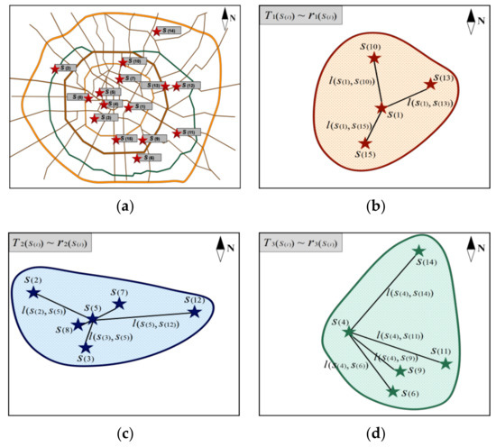
Figure 4. The tourist attraction distribution and clusters, structure trees, and spatial buffers of the clusters. (a) is the tourist attraction distribution. (b–d) are the visualization results of the structure trees and spatial buffers for the clusters $S_{(1)}$–$S_{(3)}$.

4.3. The Output Result of the Tourist Attractions and Tour Route

Considering the daytrip example, we chose two tourists as the research objects. Table 3 shows the attribute label values based on the tourist interests. The last two indices were the longitude and latitude of the starting point for each tourist. The first tourist sample $T_{(1)}$ chose to use a bicycle for transportation, while the second tourist sample $T_{(2)}$ chose to use a taxi service.

Table 3. The normalization values of tourist samples’ interest labels.

	${n_1}_{(1)}$	${n_1}_{(2)}$	${n_1}_{(3)}$	${n_1}_{(4)}$	${n_2}_{(1)}$	${n_2}_{(2)}$
$T_{(1)}$	0.10	0.90	0.90	0.30	104.052	30.634
$T_{(2)}$	0.20	0.90	1.00	0.50	104.073	30.697

4.3.1. The Analyzed Results of the Interest-Matching Objective Function Values

Based on the output cluster results and the tourist interest data, the interest-matching objective function ${\xi }_{(N,T)}$ values between the tourist interests and each tourist attraction were calculated, as shown in Table 4.

Table 4. The interest-matching objective function ${\xi }_{(N,T)}$ values between the tourist samples and each tourist attraction.

$T_{(1)}$					$T_{(2)}$
$s_{(1)}$	$s_{(2)}$	$s_{(3)}$	$s_{(4)}$	$s_{(5)}$	$s_{(1)}$	$s_{(2)}$	$s_{(3)}$	$s_{(4)}$	$s_{(5)}$
0.736	0.763	0.750	0.793	0.769	0.884	0.924	0.920	0.975	0.945
$s_{(6)}$	$s_{(7)}$	$s_{(8)}$	$s_{(9)}$	$s_{(10)}$	$s(6)$	$s(7)$	$s(8)$	$s(9)$	$s(10)$
0.966	0.809	0.802	0.812	0.748	1.131	0.976	0.969	0.991	0.893
$s_{(11)}$	$s_{(12)}$	$s_{(13)}$	$s_{(14)}$	$s_{(15)}$	$s_{(11)}$	$s_{(12)}$	$s_{(13)}$	$s_{(14)}$	$s_{(15)}$
0.814	0.793	0.770	0.685	0.903	0.992	0.962	0.911	0.868	1.039

4.3.2. The Sequencing Results of Interest-Matching Objective Function Values

Based on the data shown in Table 4, the results were provided in ascending order values of function ${\xi }_{(N,T)}$ in the sequence of the clusters, as shown in Table 5.

Table 5. The interest-matching objective function ${\xi }_{(N,T)}$ ascending values between the tourist samples and the cluster tourist attractions.

$T_{(1)}$							$T_{(2)}$
$S_{(1)}$	$s_{(1)}$	$s_{(10)}$	$s_{(13)}$	$s_{(15)}$			$S_{(1)}$	$s_{(1)}$	$s_{(10)}$	$s_{(13)}$	$s_{(15)}$
	0.736	0.748	0.770	0.903				0.884	0.893	0.911	1.039
$S_{(2)}$	$s_{(3)}$	$s_{(2)}$	$s_{(5)}$	$s_{(12)}$	$s_{(8)}$	$s_{(7)}$	$S_{(2)}$	$s_{(3)}$	$s_{(2)}$	$s_{(5)}$	$s_{(12)}$	$s_{(8)}$	$s_{(7)}$
	0.750	0.763	0.769	0.793	0.802	0.809		0.920	0.924	0.945	0.962	0.969	0.976
$S_{(3)}$	$s_{(14)}$	$s_{(4)}$	$s_{(9)}$	$s_{(11)}$	$s_{(6)}$		$S_{(3)}$	$s_{(14)}$	$s_{(4)}$	$s_{(9)}$	$s_{(11)}$	$s_{(6)}$
	0.685	0.793	0.812	0.814	0.966			0.868	0.975	0.991	0.992	1.131

(1)

Figure 5a shows the function ${\xi }_{(N,T)}$ value distribution of the first tourist in the sequence of the tourist attraction footnotes in the research domain $S$.

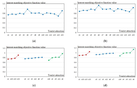Figure 5. The interest-matching objective function ${\xi }_{(N,T)}$ between the tourist samples and the tourist attractions. (a) shows the interest-matching objective function ${\xi }_{(N,T)}$ of the first tourist. (b) shows the interest-matching objective function ${\xi }_{(N,T)}$ of the second tourist. (c) shows the interest-matching objective function ${\xi }_{(N,T)}$ of the first tourist in the cluster sequence. (d) shows the interest-matching objective function ${\xi }_{(N,T)}$ of the second tourist in the cluster sequence.

(2)

Figure 5b shows the function ${\xi }_{(N,T)}$ value distribution of the second tourist in the sequence of the tourist attraction footnotes in the research domain $S$.

(3)

Figure 5c shows the function ${\xi }_{(N,T)}$ value of the first tourist according to the tourist attraction storage sequence of the interest-matching objective function matrix $P\xi (N,T)$.

(4)

Figure 5d shows the function ${\xi }_{(N,T)}$ value of the second tourist according to the tourist attraction storage sequence of the interest-matching objective function matrix $P\xi (N,T)$.

In Figure 5c,d, in the cluster sequences, the tourist attraction objective function values in each cluster are listed in the ascending order in which the red curve represents the cluster $S_{(1)}$, the blue curve represents the cluster $S_{(2)}$, and the green curve represents the cluster $S_{(3)}$.

4.3.3. The Results of the Tourist Attractions and Tour-Route Planning

According to the data in Table 3 for a one-day tour, the travel-time allowance for the first tourist sample was 9 h and the cost budget was CNY 300 yuan. The travel-time allowance for the second tourist sample was 11 h and the cost budget was CNY 500 yuan. The first tourist chose to take the bicycle while the second tourist chose to take the taxi. Based on the proposed algorithm, a potential tourist attraction itinerary and tour route that was based on each tourist sample’s interests and their chosen modes of transportation (i.e., bicycle and taxi service, respectively) were identified, as shown in Table 6.

Table 6. The tourist attractions and tour route that best match the tourists’ interests.

	$S_t$	$Q_{(0)}$	$s_{(14)}$	$Q_{(1)}$	$s_{(1)}$	$Q_{(2)}$	$s_{(6)}$	Total
$T_{(1)}$	0/0	0.80/6.0	3.0/20.0	0.62/4.0	3.0/0	0.35/3.0	1.0/0	8.77/33.0
	$S_t$	$Q_{(0)}$	$s_{(14)}$	$Q_{(1)}$	$s_{(1)}$	$Q_{(2)}$	$s_{(6)}$	$Q_{(3)}$	$s_{(3)}$	Total
$T_{(2)}$	0/0	0.27/14.0	3.0/20.0	0.38/22.0	3.0/0	0.32/14.0	1.0/0	0.28/16.0	2.0/50.0	10.25/136

Table 6 shows the results of the tourist attraction element $T_{s(i)}$ of the tour-route searching steady vector $T_s$ and the cost iteration sub-unit $Q_{(i)}$. The values were the required time (unit: hour) and the minimum cost (unit: CNY yuan) to visit the tourist attractions. The values between the two tourist attractions represented the travel time (unit: hour) and minimum travel cost (unit: CNY yuan) in the cost iteration sub-unit $Q_{(i)}$ under the condition of the chosen transportation mode. It also shows the optimal tourist attractions and tour route based on the tourists’ requirements.

4.4. The Comparison Results of the Algorithms

To verify the results of the proposed algorithm, a control set of algorithms were conducted under the same experimental conditions and their results compared with those of the proposed algorithm.

4.4.1. Selecting and Confirming of the Control Algorithms

In tourism research, shortest-path algorithms such as the Dijkstra and A* algorithms have typically been used to plan tour routes with the shortest traveling distances. They have the benefits of being easily accessed and applied [40,41,42]. In addition, the shortest-path algorithms were also constrained by tourism factors such as features and spatial attributes. Once the traveling distances between the tourist attractions have been defined by the city roads and road nodes, the shortest-path algorithms can operate. Since the proposed algorithm’s experimental environment conforms to these conditions, the Dijkstra algorithm and the A* algorithm were chosen as controls to plan the travel routes for the sub-unit $\Phi$, and the control group algorithms were defined as Algorithm 1 (A1) and Algorithm 2 (A2). Under the same conditions of the algorithm operating time and the interest data of the two tourist samples, the control group algorithms were used to dynamically search the same tourist attractions, cost iteration sub-units, and tour routes. Their results of were then compared with those of the proposed algorithm (PA), as shown in Table 7, in which the first tourist chose cycling, the second tourist chose a taxi service.

Table 7. The tourist attractions and the tour routes that best match tourist interests under the condition of the three algorithms.

PA		$S_t$	$Q_{(0)}$	$s_{(14)}$	$Q_{(1)}$	$s_{(1)}$	$Q_{(2)}$	$s_{(6)}$	Total
	$T_{(1)}$	0/0	0.80/6.0	3.0/20.0	0.62/4.0	3.0/0	0.35/3.0	1.0/0	8.77/33.0
		$S_t$	$Q_{(0)}$	$s_{(14)}$	$Q_{(1)}$	$s_{(1)}$	$Q_{(2)}$	$s_{(6)}$	$Q_{(3)}$	$s_{(3)}$	Total
	$T_{(2)}$	0/0	0.27/14.0	3.0/20.0	0.38/22.0	3.0/0	0.32/14.0	1.0/0	0.28/16.0	2.0/50.0	10.25/136
A1		$S_t$	$Q_{(0)}$	$s_{(14)}$	$Q_{(1)}$	$s_{(1)}$	$Q_{(2)}$	$s_{(6)}$	Total
	$T_{(1)}$	0/0	0.95/7.5	3.0/20.0	0.73/5.0	3.0/0	0.46/4.0	1.0/0	9.14/36.5
		$S_t$	$Q_{(0)}$	$s_{(14)}$	$Q_{(1)}$	$s_{(1)}$	$Q_{(2)}$	$S_{(6)}$	$Q_{(3)}$	$s_{(3)}$	Total
	$T_{(2)}$	0/0	0.32/15.0	3.0/20.0	0.47/25.0	3.0/0	0.38/17.0	1.0/0	0.38/20.0	2.0/50.0	10.55/147
A2		$S_t$	$Q_{\left(0\right)}$	$S_{\left(14\right)}$	$Q_{\left(1\right)}$	$S_{\left(1\right)}$	$Q_{\left(2\right)}$	$S_{\left(6\right)}$	Total
	$T_{\left(1\right)}$	0/0	1.00/7.5	3.0/20.0	0.75/5.5	3.0/0	0.45/4.0	1.0/0	9.2/37.0
		$S_t$	$Q_{\left(0\right)}$	$S_{\left(14\right)}$	$Q_{(1)}$	$s_{(1)}$	$Q_{(2)}$	$S_{(6)}$	$Q_{(3)}$	$s_{(3)}$	Total
	$T_{(2)}$	0/0	0.36/18.0	3.0/20.0	0.43/23.0	3.0/0	0.33/15.0	1.0/0	0.32/19.0	2.0/50.0	10.44/145

4.4.2. The Comparison Results of the Proposed Algorithm with the Control Algorithms

Table 7 shows the element tourist attractions $T_{s(i)}$ of the steady matrix $T_s$ and the cost iteration sub-units $Q_{(i)}$ under the condition of each algorithm. The values between the two tourist attractions represent the travel time (unit: hour) and minimum moving cost (unit: CNY yuan) in the cost iteration sub-unit $Q_{(i)}$ with the chosen transportation modes. According to Table 7, the Figure 6 curve results were as follows:

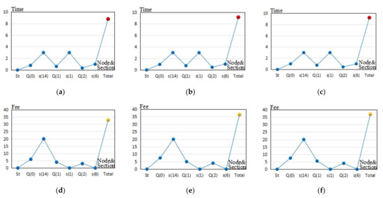
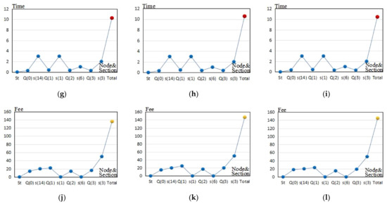
Figure 6. The time- and fee-cost deduction and fluctuating tendency of each algorithm for the two tourist samples. (a–c) are the deduction and fluctuating tendency of the visiting tourist attraction time, travel time between two tourist attractions, and the total time of the proposed algorithm, Algorithm 1, and Algorithm 2, respectively, for the first tourist sample. (d–f) are the deduction and fluctuating tendency of the visiting tourist attraction fee, travel fee between two tourist attractions, and the total costs of the proposed algorithm, Algorithm 1, and Algorithm 2, respectively, for the first tourist sample. (g–i) are the deduction and fluctuating tendency of the visiting tourist attraction time, travel time between two tourist attractions, and the total time of the proposed algorithm, Algorithm 1, and Algorithm 2, respectively, for the second tourist sample. (j–l) are the deduction and fluctuating tendency of the visiting tourist attraction fee, travel fee between two tourist attractions, and the total costs consuming of the proposed algorithm, Algorithm 1, and Algorithm 2, respectively, for the second tourist sample.

(1)

Figure 6a–c shows the deduction and fluctuating tendency of the visiting tourist attraction time, travel time between two tourist attractions, and the total time of the PA, A1, and A2 for the first tourist sample.

(2)

Figure 6d–f shows the deduction and fluctuating tendency of the visiting tourist attraction fee, travel costs between two tourist attractions, and the total costs of the PA, A1, and A2 for the first tourist sample.

(3)

Figure 6g–i shows the deduction and fluctuating tendency of the visiting tourist attraction time, travel time between two tourist attractions, and the total time of the PA, A1, and A2 for the second tourist sample.

(4)

Figure 6j–l shows the deduction and fluctuating tendency of the visiting tourist attraction fee, travel costs between two tourist attractions, and the total costs of the PA, A1, and A2 for the second tourist sample.

In each figure, the red and yellow dots represent the total time and total costs, respectively.

(5)

Figure 7a,b shows the comparison of each algorithm on the total time and the total costs for the first tourist under the condition of the first tourist’s interest data and the same tourist attractions and cost sub-units.

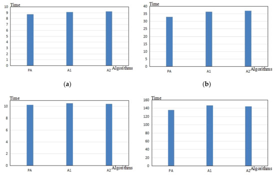Figure 7. The comparison of the total time and costs of the tour routes for the two tourist samples. (a,b) shows the comparison of each algorithm on the total time and the total costs for the first tourist under the condition of the first tourist’s interest data and the same tourist attractions and cost sub-units. (c,d) shows the comparison of each algorithm on the total time and the total fee cost for the second tourist under the condition of the second tourist’s interest data and the same tourist attractions and cost sub-units.

(6)

Figure 7c,d shows the comparison of each algorithm on the total time and the total costs for the second tourist under the condition of the second tourist’s interest data and the same tourist attractions and cost sub-units.

With regard to the computer algorithm optimization, when searching for the shortest route, the Dijkstra algorithm has low efficiency. Compared to the Dijkstra algorithm, the heuristic function is introduced to the A* algorithm, to some extent, the algorithm efficiency was improved. In comparison, the proposed algorithm is based on multiple dot parallel searching, it has higher operating efficiency, and consumes smaller operating space than the Dijkstra algorithm and A* algorithm. Table 8 shows the comparison of the Dijkstra algorithm, A* algorithm, and the proposed algorithm with regard to the time complexity (TC) and space complexity (SC). The data in the table shows the TC and SC examples when the tourist attraction numbers are $n=4$, $n=5$, and $n=6$. The symbol ${\rho }_{1,1}$ represents the TC ratio between the Dijkstra algorithm and the proposed algorithm, the symbol ${\rho }_{1,2}$ represents the SC ratio between the Dijkstra algorithm and the proposed algorithm. The symbol ${\rho }_{2,1}$ represents the TC ratio between the A* algorithm and the proposed algorithm, the symbol ${\rho }_{2,2}$ represents the SC ratio between the A* algorithm and the proposed algorithm.

Table 8. The comparison of the Dijkstra algorithm, A* algorithm, and the proposed algorithm on the aspect of time complexity (TC) and space complexity (SC).

	TC						SC
	$n$	$n=4$	$n=5$	$n=6$	$\rho$		$n$	$n=4$	$n=5$	$n=6$	$\rho$
A1	$O(n{\log }_{2}n+n^2)$	$O(24)$	$O(36.61)$	$O(51.51)$	${\rho }_{1,1}>1$	A1	$O(n)$	$O(4)$	$O(5)$	$O(6)$	${\rho }_{1,2}>1$
A2	$O(n{\log }_{2}n+n)$	$O(12)$	$O(16.61)$	$O(21.51)$	${\rho }_{2,1}>1$	A2	$O(1)$		$O(1)$	$O(1)$	${\rho }_{2,2}>1$
PA	$O(n{\log }_{2}n)$	$O(8)$	$O(11.61)$	$O(15.51)$		PA	$O(1)$	$O(1)$	$O(1)$	$O(1)$

4.5. The Analysis and Conclusions of the Experiment Results

4.5.1. The Analysis and Conclusion on the Collection Results of the Tourist Attractions and Tourist Attraction Attributes

After analyzing Section 4.1 and Table 1 data, the following conclusions were reached.

(1)

The tourist attractions that were chosen in the experiment conformed to the preset conditions of the proposed algorithm.

(2)

The tourist attractions were popular tourist attractions in Chengdu City with typical features and spatial attributes. Each tourist attraction had different attributes that affected their capacity to satisfy varying tourist interests, which formed the clustering condition. In addition, they were located across the city, which formed the spatial modeling condition.

(3)

Table 1 data were used to generate clusters and interest-matching objective functions. The data were normalized values that were processed by the feature attribute label vector normalization parameter ${\delta }_{1(i1)}$, and they conformed to the proposed algorithm conditions.

4.5.2. The Analysis and Conclusion of the Results of Clustering and Cluster Visualization

After analyzing Section 4.2, Table 2 data, and Figure 4, the following conclusions were reached.

(1)

In Table 2, the clustering objective function values between the two different tourist attractions were all different. They represented the degree of correlation among the two different tourist attractions.

(2)

Via the proposed algorithm, three tourist attraction clusters were identified.

(3)

The tourist attractions in the same cluster had a high degree of correlation among their attributes and the objective function values were relatively small. The tourist attractions in different clusters had a low degree of correlation among their attributes and the objective function values were relatively large.

(4)

The Figure 4 shows the formed three clusters, cluster structure trees, and cluster spatial buffers that were constrained by the proposed algorithm.

①

Figure 4a shows the distribution of all the tourist attraction samples with note labels. They were spatially discrete.

②

As to the inner tree structure of the clusters: in Figure 4b, the topological connecting lines among tourist attractions formed the first structure tree and it indicated the searching process of the first cluster. In Figure 4c, the topological connecting lines among the tourist attractions formed the second structure tree, and it indicated the searching process of the second cluster. In Figure 4d, the topological connecting lines among the tourist attractions formed the third structure tree, and it indicated the searching process of the third cluster.

③

As to the structure of the cluster buffer: in Figure 4b, the closed brown space was the first cluster spatial buffer and indicated the spatial range of the first cluster. In Figure 4c, the closed blue space was the second cluster spatial buffer and indicated the spatial range of the second cluster. In Figure 4d, the closed green space was the third cluster spatial buffer and indicated the spatial range of the third cluster.

(5)

Since the proposed algorithm combined spatial attributes, the three structure trees and buffers each had different shapes and topology tendencies, which visually indicated that different clusters not only had discrepancies in feature attributes but had larger discrepancies in their spatial attributes. In addition, the three clusters had spatial overlap in the city range. It indicated that the correlation relationship among the tourist attractions in the clusters as relative but not isolated. The formed tour routes could pass through different clusters.

4.5.3. The Analysis and Conclusion on the Results of the Tourist Attractions and Tour Route

After analyzing Section 4.3, Table 3, Table 4, Table 5 and Table 6 data, and Figure 5, the following conclusions were reached.

(1)

Table 3 shows the normalized data of the two tourist interest labels. It indicated that the two tourists had completely different interests. In addition, the starting points for the two tourists were different. According to the proposed algorithm, the precondition in Table 3 differentiated the results of the two tourists and followed the experimental logic.

(2)

Table 4 shows the interest-matching objective function values between the two tourist samples with each tourist attraction.

①

The values were different due to Table 3 preconditions and the operation of the proposed algorithm. It indicated that each tourist attraction’s capacity on satisfying tourist’s interests would be different. The tourist attraction that had the stronger capacity would be preferentially selected as the tour-route tourist attraction.

②

Upon further interpretation, the smaller the value was, the closer the tourist attraction attributes were to the tourist’s interests and the tourist attraction would be more likely to satisfy the tourist. On the contrary, the bigger the value was, the more remote the tourist attraction attributes were to the tourist’s interests and the tourist attraction would be less likely to satisfy the tourist.

(3)

Table 5 was deduced from Table 4. It shows that each tourist attraction was stored in the matrix $P_{\xi (N,T)}$ in the ascending order of the interest-matching objective function value. It indicated the capacity sequence of each tourist attraction on satisfying tourist interests.

(4)

Figure 5 was deduced from Table 3, Table 4 and Table 5, and it indicated that the interest-matching objective function values had the fluctuate tendency and the tourist attraction capacities varied with the footnotes in each cluster.

As to the first tourist, the interest-matching objective function values are shown in the Figure 5a,c:

(1)

Tourist attraction $s_{(6)}$: East Lake Park had the highest matching function value and we interpreted that it had the lowest capacity for satisfying the tourist’s interests.

(2)

Tourist attraction $s_{(14)}$: Chengdu Zoo had the lowest matching function value, and we interpreted that it had the highest capacity for satisfying the tourist’s interests.

(3)

In the cluster $S_{(1)}$, tourist attraction $s_{(1)}$: Chunxi Road and Zhongshan Square had the highest capacity on satisfying the tourist’s interests; The tourist attraction $s_{(15)}$: Raffles Square had the lowest capacity for satisfying the tourist’s interests.

(4)

In the cluster $S_{(2)}$, tourist attraction $s_{(3)}$: Temple of Marquis Wu had the highest capacity on satisfying the tourist’s interests; The tourist attraction $s_{(7)}$: Wenshu Temple had the lowest capacity for satisfying the tourist’s interests.

(5)

In the cluster $S_{(3)}$, tourist attraction $s_{(14)}$: Chengdu Zoo had the highest capacity for satisfying the tourist’s interests; The tourist attraction $s_{(6)}$: East Lake Park had the lowest capacity for satisfying the tourist’s interests.

As to the second tourist, the interest-matching objective function values are shown in the Figure 5b,d.

(1)

Tourist attraction $s_{(6)}$: East Lake Park had the highest matching function value, and we interpreted that it had the lowest capacity for satisfying the tourist’s interests.

(2)

Tourist attraction $s_{(14)}$: Chengdu Zoo had the lowest matching function value, and we interpreted that it had the highest capacity for satisfying the tourist’s interests.

(3)

In the cluster $S_{(1)}$, tourist attraction $s_{(1)}$: Chunxi Road and Zhongshan Square had the highest capacity for satisfying the tourist’s interests; The tourist attraction $s_{(15)}$: Raffles Square had the lowest capacity for satisfying the tourist’s interests.

(4)

In cluster $S_{(2)}$, tourist attraction $s_{(3)}$: Temple of Marquis Wu had the highest capacity for satisfying the tourist’s interests; The tourist attraction $s_{(7)}$: Wenshu Temple had the lowest capacity for satisfying the tourist’s interests.

(5)

In cluster $S_{(3)}$, tourist attraction $s_{(14)}$: Chengdu Zoo had the highest capacity for satisfying the tourist’s interests; The tourist attraction $s_{(6)}$: East Lake Park had the lowest capacity for satisfying the tourist’s interests.

(6)

Table 6 indicated the tour route output results that were based on Table 3, Table 4 and Table 5 preconditions. The following conclusions were reached. (result interpretation 5)

①

The tourist attractions of the two tour routes all matched the tourist interests.

②

The recommended tour route for the first tourist was 8.77 h long and cost CNY 33 yuan. We interpreted that the proposed algorithm’s tour route results conformed to the tourist’s requirements.

③

The recommended tour route for the second tourist was 10.25 h long and cost CNY 136 yuan. We interpreted that the proposed algorithm’s tour route conformed to the tourist’s requirements.

④

The total time and costs were within the ranges of the tourists’ allowances and met their needs. We interpreted that the algorithm was feasible and accurate.

4.5.4. The Analysis and Conclusion on the Comparison Result of the Algorithms

After analyzing Section 4.4, Table 7, Table 8, and Figure 6 and Figure 7, the following conclusions were reached.

(1)

The controls that were used were the Dijkstra and A* algorithms, as they have both been used extensively for shortest-path calculations and for planning optimal tour routes. Therefore, the control group algorithms were feasible, accessible, and comparable.

(2)

Due to the different preconditions on tourist interests, starting points, time, costs, and their chosen modes of transportation, the first tourist had three recommended tourist attractions while the second tourist had four recommendations. We interpreted that when the preconditions changed, the results of the proposed algorithm and the control algorithms changed as well.

(3)

All three algorithms produced fluctuating time durations and costs for visiting various tourist attractions and traveling between two tourist attractions. Each algorithm resulted in different values for these variables. The differences are caused by the preconditions of the tourists’ needs, tourist attraction attributes, and city geospatial environment, and were also caused by the three algorithms’ different performances.

①

The tour routes by the Dijkstra and A* algorithms were less efficient and more expensive than those by the proposed algorithm. We interpreted that the proposed algorithm had an advantage on saving time and costs when planning tour routes, as compared to the controls.

②

From the Table 8, it can be concluded that the three algorithms had different performances. On the aspect of computer algorithm performance, when searching the shortest tour route, the proposed algorithm had much lower time complexity and space complexity than the Dijkstra algorithm, while it had much lower time complexity than the A* algorithm and had the same dimension of space complexity with the A* algorithm. Through the mathematical calculating, the ratio $\rho$ was obtained. When the tourist attraction number $n$ was larger than 2, the ratios ${\rho }_{1,1}$, ${\rho }_{1,2}$, ${\rho }_{2,1}$, and ${\rho }_{2,2}$ were all larger than 1. It can be concluded that when tourist attractions are confirmed in the searching process on the shortest tour route, the Dijkstra and A* algorithm always consumed higher time complexity and space complexity than the proposed algorithm, and the Dijkstra algorithm always consumed higher time complexity than the proposed algorithm while the A* algorithm consumed the same dimension of space complexity with the proposed algorithm.

③

Under the condition of the small tourist attraction data set, the proposed algorithm relied on an exhaustive method, and thus it found global optimal solutions. The Dijkstra and A* algorithms rely on local “greedy” search methods, they might easily converge on a local optimal solution and consume more time complexity and space complexity. In one complete tour route, the larger number of tourist attraction is, the more computer operating time and computer space will be required. That is, the weaker the algorithm performance is, the more time complexity and space complexity will be needed to search the optimal solution. In the experiment, when the three algorithms were carried out under the same computer operating times, the proposed algorithm would find out the optimal tour route more quickly, while the control group algorithms might not find out the optimal one since the Dijkstra algorithm and the A* algorithm’s performances were not better than the proposed algorithm with regard to time complexity and space complexity, especially when the tourist attraction number is sufficiently large, the time and space consuming gap would be rapidly widened. Thus, under the conditions of the identical limited operating time and space consumption, the Dijkstra and A* algorithm are inferior to finding out the optimal solution, or even could not find it out and converge on a local optimal solution. In other words, if the Dijkstra algorithm or the A* algorithm are set as the embedded algorithm of the smart tourism system, they can also find out the optimal tour route, but they will consume more computer operating time and space. In all, the proposed algorithm had a better performance than the Dijkstra and A* algorithms in searching optimal tour routes.

(4)

In Figure 7, the following conclusions were reached.

①

With regard to the first tourist, the proposed algorithm route was 8.77 h long and cost CNY 33 yuan. The Dijkstra algorithm route was 9.14 h long and cost CNY 36.5 yuan. The A* algorithm route was 9.2 h long and cost CNY 37 yuan. We interpreted that the proposed algorithm was superior to the control algorithms.

②

With regard to the second tourist, the proposed algorithm route was 10.25 h long and cost CYN 136 yuan. The Dijkstra algorithm route was 10.55 h long and cost CYN 147 yuan. The A* algorithm route was 10.44 h long and cost CYN 145 yuan. We interpreted that the proposed algorithm was superior to the control algorithms.

③

For the first tourist, the time duration of the tour routes that were recommended by the Dijkstra and A* algorithms both exceeded the nine hours, and thus the results did not conform to the tourist’s allowance. In this aspect, we interpreted that the control algorithms were inferior to the proposed algorithm.

5. Conclusions

5.1. Contribution

Based on the current challenges in tour-route planning and attraction recommendations, this study designed a tour-route planning and recommendation algorithm that was based on an improved AGNES spatial clustering and space-time deduction model. This model improved interest-matching, urban-tourist-attraction clustering, space-time deduction, and tour-route planning based on various modes of transportation. By combining the tourist attraction features and spatial attributes, the improved AGNES tourist attraction clustering algorithm was created, and the cluster structure trees, cluster spatial buffers, and clusters were generated. All the tourist attractions with a high degree of correlation among the attributes were clustered together. Based on the tourist-interest data, the interest-matching objective function was created. This function reflected each tourist attraction’s capacity for satisfying the tourist’s interests, which formed the precondition when planning the tour route. Under the constraint conditions of time and cost allowance, the proposed algorithm searched for the optimal tourist attractions to match the tourist interests as well as considered the optimal tour route. The resultant tour routes met the tourists’ needs and interests. Based on the comparison results, the proposed algorithm had advantages when compared to the controls. The proposed algorithm reduced the costs and time investment for tour-route planning. The improved AGNES clustering algorithm considered spatial distance and various tourist attraction attributes. The proposed algorithm integrated mixed (i.e., preferred) transportation modes for different optimized results. Tour-route planning that was based on space-time deduction was an innovative method that not only considered the time and cost constraints, but also considered the shortest traveling distance between two tourist attractions. Therefore, the resultant tour routes satisfied the tourist’s interests and reduced the time and costs that were invested by tourists.

5.2. Addressing Challenges for Research

Smart mobile devices have become part of daily life, and, for many applications, activities and events are planned using smart mobile devices. Mobile planning is the key to ensuring efficient routing, resource allocation, and energy management. For example, the researchers in [30] considered that efficient routing, resource allocation, and energy management could be achieved through clustering of mobile nodes into local groups. In the study, a clustering scheme was developed to prolong the network lifetime by distributing energy consumption among clusters. In [31], a novel travel route recommendation system was proposed that collected tourist on-site travel behavior data automatically regarding a specific POI that was based on smart phone and Internet of Things technologies. The tour-route-recommendation algorithm was then created to search and rank the tangible travel routes. The researchers in [32] considered that the prevalence of smart mobile devices and location-based services would lead to an increasing volume of mobility data. Based on big mobile data, it proposed a method for accurately predicting the next location of a traveling object.

In tourism activities, tourists’ traveling behaviors also generate massive amounts of data on mobile devices. How to appropriately and accurately use these data is a future challenge for tourism research. Mobile data could be used in tourism data mining, tourist attraction location, tourist interest tendency research, tourism facility evaluations, tour-route planning, and recommendations, etc. It has been deemed the most important, challenging, and valuable research field for the future. How to precisely optimize mobile data acquisition, mine interest data, match tourists’ needs, search optimal solutions, etc., are challenges that should be addressed.

5.3. Limitation and Future Work

When searching the tour routes, the proposed algorithm sets the transportation mode, time allowance, and costs as the constraint conditions. However, the proposed algorithm still has some drawbacks and limitations. First, the AGNES clustering algorithm itself has its limitation in efficiency, accuracy, and space complexity. Second, in the tour-route algorithm, the transportation modes were relatively fixed, whereas tourists might choose different transportation modes in the tour process. Third, the proposed method did not involve mobile data; we provided a method under the condition of city tourist attractions’ attributes, tourists’ specific interests, and an urban tourism environment. Therefore, additional research could expand and validate our proposed algorithm further. First, more precise tourist attraction clustering methods could be studied, which could refine and better target the clustering results based on tourist interests. The clustering objective function criteria and model procedure could be refined further as well. The criteria to select the parameters could add more factors to satisfy more individualized interests. Second, the transportation mode selection for the whole tour should be more flexible and random, which could then consider tourist selection tendency on different cost deduction sub-units between two tourist attractions. In further research, we will study random transportation mode selection in different sub-units, and a more individualized tour-route-searching algorithm will be designed and proposed. Third, mobile data should be used to mine tourist interests and to integrate specialized interests. To some extent, a smart tourism recommendation system could be set up by mining historical tourists’ data and find related knowledge.

References

- Kaufman, L.; Rousseeuw, P.J. Finding Groups in Data: An Introduction to Cluster Analysis; John Wiley & Sons: Hoboken, NJ, USA, 2009; Volume 344. [Google Scholar]
- Sano, A.V.D.; Imanuel, T.D.; Calista, M.I.; Nindito, H.; Condrobimo, A.R. The Application of AGNES Algorithm to Optimize Knowledge Base for Tourism Chatbot. In Proceedings of the 2018 International Conference on Information Management and Technology, Bina Nusantara University, Jakarta, Indonesia, 3–5 September 2018; pp. 65–68. [Google Scholar]
- Rocha, J.M.P.; Alcaraz, J.A.S.; Rodriguez, R.G.; Sifuentes, O.J.P.; Espinal, A.; Figueroa, M.A.S. Application of Agglomerative and Partitional Algorithms for the Study of the Phenomenon of the Collaborative Economy within the Tourism Industry. J. Autom. Mob. Robot. Intell. Syst. 2020, 14, 81–86. [Google Scholar]
- Valls, A.; Gibert, K.; Orellana, A.; Antón-Clavé, S. Using ontology-based clustering to understand the push and pull factors for British tourists visiting a Mediterranean coastal destination. Inf. Manag. 2018, 55, 145–159. [Google Scholar] [CrossRef]
- Loiseau, T.J.; Djebali, S.; Raimbault, T.; Branchet, B.; Chareyron, G. Characterization of daily tourism behaviors based on place sequence analysis from photo sharing websites. In Proceedings of the 2017 IEEE International Conference on Big Data, Boston, MA, USA, 11–14 December 2017; pp. 2760–2765. [Google Scholar]
- Yi, Y.T. Design of Intelligent Recommendation APP for Ecotourism Routes Based on Popular Data Clustering of Points of Interest. In Proceedings of the Second International Conference on Smart Electronics and Communication, Chennai, Tamil Nadu, India, 7–9 October 2021; pp. 1270–1273. [Google Scholar]
- Hu, S.; Chau, P.M.; Weng, J.; Lin, P.; Zhou, W. Extending the Theory of Planned Behavior to Explore the Influence of Residents’ Dependence on Public Transport. IEEE Access 2021, 9, 137224–137240. [Google Scholar] [CrossRef]
- Zahra, A.M.; Hamed, V.N.; Javad, S. Tourism recommendation system based on semantic clustering and sentiment analysis. Expert Syst. Appl. 2021, 167, 114324. [Google Scholar]
- Retnosari, M.; Wasino; Arisandi, D. Tourism Destination Grouping Systems With Partitioning Clustering Method from Geotagged Photo using Android. IOP Conf. Ser. Mater. Sci. Eng. 2020, 852, 012160. [Google Scholar] [CrossRef]
- Majewska, J.; Truskolaski, S. Cluster-mapping procedure for tourism regions based on geostatistics and fuzzy clustering: Example of Polish districts. Curr. Issues Tour. 2019, 22, 2365–2385. [Google Scholar] [CrossRef]
- Darmawiguna, I.G.M.; Pradnyana, G.A.; Santyadiputra, G.S. The Development of Integrated Bali Tourism Information Portal using Web Scrapping and Clustering Methods. J. Phys. Conf. Ser. 2019, 1165, 012010. [Google Scholar] [CrossRef]
- Deng, N.; Liu, J. Where did you take those photos? Tourists’ preference clustering based on facial and background recognition. J. Destin. Mark. Manag. 2021, 21, 100632. [Google Scholar] [CrossRef]
- Lee, H.; Kang, Y. Mining tourists’ destinations and preferences through LSTM-based text classification and spatial clustering using Flickr data. Spat. Inf. Res. 2021, 29, 825–839. [Google Scholar] [CrossRef]
- Rodriguez-Echeverria, J.; Semanjski, I.; Van Gheluwe, C.; Ochoa, D.; Ijben, H.; Gautama, S. Density-Based Spatial Clustering and Ordering Points Approach for Characterizations of Tourist Behaviour. ISPRS Int. J. Geo-Inf. 2020, 9, 686. [Google Scholar] [CrossRef]
- Kirilenko, A.P.; Stepchenkova, S.; Hernandez, J.M. Comparative clustering of destination attractions for different origin markets with network and spatial analyses of online reviews. Tour. Manag. 2018, 72, 400–410. [Google Scholar] [CrossRef]
- Hong, M.; Jung, J.J. Multi-criteria tensor model consolidating spatial and temporal information for tourism recommendation. J. Amb. Intel. Smart. Environ. 2020, 13, 5–19. [Google Scholar] [CrossRef]
- Han, S.; Liu, C.; Chen, K.; Gui, D.; Du, Q. A Tourist Attraction Recommendation Model Fusing Spatial, Temporal, and Visual Embeddings for Flickr-Geotagged Photos. ISPRS Int. J. Geo-Inf. 2021, 10, 20. [Google Scholar] [CrossRef]
- Zheng, W.; Liao, Z.; Lin, Z. Navigating through the complex transport system: A heuristic approach for city tourism recommendation. Tour. Manag. 2020, 81, 104162. [Google Scholar] [CrossRef]
- Seo, J.C.; Hwan, R.K.; Yong, L.J.; Dong, J.K. Deep Learning-based Tourism Recommendation System using Social Network Analysis. Int. J. Internet Broadcasting Commun. 2020, 12, 113–119. [Google Scholar]
- Borade, J.; Makwana, S.; Gupta, P.; Lanjewar, S. Intelligent Agent for Tourism Recommendation System. Int. J. Res. Eng.Technol. 2018, 7. [Google Scholar] [CrossRef]
- Santos, F.; Almeida, A.; Martins, C.; Gonçalves, R.; Martins, J. Using POI functionality and accessibility levels for delivering personalized tourism recommendations. Comput. Environ. Urban Syst. 2017, 77, 101173. [Google Scholar] [CrossRef]
- Zhang, Z.; Pan, H.; Xu, G.; Wang, Y.; Zhang, P. A Context-Awareness Personalized Tourist Attraction Recommendation Algorithm. Cybern. Inf. Technol. 2016, 16, 146–159. [Google Scholar] [CrossRef] [Green Version]
- Ai, J. Research on individualized travel route recommendation based on improved collaborative filtering technology. Mod. Electron. Technol. 2019, 42, 182–186. [Google Scholar]
- Xiao, C.; Xia, K.; Qiao, Y.; Zhang, Y. Tourism route recommendation based on dynamic clustering. J. Comput. Appl. 2017, 37, 2395–2400. [Google Scholar]
- Song, W. Research on Mobile Tourism Route Recommendation Model Based on Optimized Social Tags and Association Rules Algorithm. Master’s Thesis, Guilin University of Technology, Guilin, China, 2019. [Google Scholar]
- Wu, J. Research and Implementation of Personalized Travel Recommendation System Based on Collaborative Filtering Recommendation. Master’s Thesis, Beijing Jiaotong University, Beijing, China, 2017. [Google Scholar]
- Chen, G. Research and Implementation of Group Travel Recommendation Algorithm Based on Geo-Tag and Time Factor. Master’s Thesis, Beijing University of Posts and Telecommunications, Beijing, China, 2019. [Google Scholar]
- Chen, Y.; Wu, S.; Dong, C. Tourist route recommendation under the constraints of personal time and space behavior. J. Green Sci. Technol. 2018, 11, 100. [Google Scholar]
- Li, D. Design and Implementation of Travel Recommendation System Based on Hybrid Recommendation Algorithm. Master’s Thesis, Zhejiang University, Hangzhou, Zhejiang Province, China, 2018. [Google Scholar]
- Comito, C.; Talia, D.; Trunfio, P. An Energy-Aware Clustering Scheme for Mobile Applications. In Proceedings of the 2011 IEEE 11th International Conference on Computer and Information Technology, Paphos, Cyprus, 31 August–2 September 2011; pp. 15–22. [Google Scholar]
- Bin, C.; Gu, T.; Sun, Y.; Chang, L.; Sun, L. A Travel Route Recommendation System Based on Smart Phones and IoT Environment. Wirel. Commun. Mob. Comput. 2019, 2019, 7038259. [Google Scholar] [CrossRef] [Green Version]
- Monreale, A.; Pinelli, F.; Trasarti, R.; Giannotti, F. WhereNext: A location predictor on trajectory pattern mining. In Proceedings of the 15th ACM SIGKDD International Conference on Knowledge Discovery and Data Mining, Paris, France, 28 June–1 July 2009. [Google Scholar]
- Zhou, X.; Xu, C.; Kimmons, B. Detecting tourism destinations using scalable geospatial analysis based on cloud computing platform. Comput. Environ. Urban Syst. 2015, 54, 144–153. [Google Scholar] [CrossRef]
- Zhao, S.; Zhao, T.; King, I.; Lyu, M.R. Geo-teaser: Geo-temporal sequential embedding rank for point-of-interest recommendation. In Proceedings of the 26th International Conference on World Wide Web Companion, Geneva, Switzerland, 3–7 April 2017; pp. 153–162. [Google Scholar]
- Young, C.; Young, U.R.; Kyeong, K. A Recommender System based on Personal Constraints for Smart Tourism City. Asia Pac. J. Tour. Res. 2021, 26, 440–453. [Google Scholar]
- Jabbarpour, M.R.; Noor, R.M.; Khokhar, R.H. Green vehicle traffic routing system using ant-based algorithm. J. Netw. Comput. Appl. 2015, 58, 294–308. [Google Scholar] [CrossRef]
- Li, D.; Yu, Z.; Luo, W.; Hu, Y.; Che, X.; Yuan, L. Optimal route searching with multiple dynamical constraints—A geometric algebra approach. ISPRS Int. J. Geo-Inf. 2018, 7, 172. [Google Scholar] [CrossRef] [Green Version]
- Lin, Q.; Chao, Y.; Yang, N. A travel routes recommendation algorithm based on user’s time constraints. Geogr. Geo-Inf. Sci. 2017, 25–29. [Google Scholar]
- Damos, M.A.; Zhu, J.; Li, W.; Hassan, A.; Khalifa, E. A novel urban tourism path planning approach based on a multiobjective genetic algorithm. ISPRS Int. J. Geo-Inf. 2021, 10, 530. [Google Scholar] [CrossRef]
- Cergibozan, Ç.; Tasan, A.S. Tourist Route Planning with a Metaheuristic Approach. In Closing the Gap between Practice and Research in Industrial Engineering; Springer: Cham, Switzerland, 2017; pp. 193–199. [Google Scholar]
- Fitriansyah, A.; Parwati, N.W.; Wardhani, D.R.; Kustian, N. Dijkstra’s Algorithm to Find Shortest Path of Tourist Destination in Bali. J. Phys. Conf. Ser. 2019, 1338, 012044. [Google Scholar] [CrossRef] [Green Version]
- Liang, Y.; Wang, L. Applying genetic algorithm and ant colony optimization algorithm into marine investigation path planning model. Soft Comput. 2019, 24, 8199–8210. [Google Scholar] [CrossRef]
Publisher’s Note: MDPI stays neutral with regard to jurisdictional claims in published maps and institutional affiliations. |
© 2022 by the authors. Licensee MDPI, Basel, Switzerland. This article is an open access article distributed under the terms and conditions of the Creative Commons Attribution (CC BY) license (https://creativecommons.org/licenses/by/4.0/).