Point Cloud Convolution Network Based on Spatial Location Correspondence

Abstract

The study of convolutional neural networks for 3D point clouds is becoming increasingly popular, and the difficulty lies mainly in the disorder and irregularity of point clouds. At present, it is straightforward to propose a convolution operation and perform experimental validation. Although good results are achieved, the principles behind them are not explained—i.e., why this can solve the disorder and irregularity of point clouds—and it is difficult for the researchers to design a point cloud convolution network suitable for their needs. For this phenomenon, we propose a point convolution network framework based on spatial location correspondence. Following the correspondence principle can guide us in designing convolution networks adapted to our needs. We analyzed the intrinsic mathematical nature of the convolution operation, and we argue that the convolution operation remains the same when the spatial location correspondence between the convolution kernel points and the convolution range elements remains unchanged. Guided by this principle, we formulated a general point convolution framework based on spatial location correspondence, which explains how to handle a disordered point cloud. Moreover, we discuss different kinds of correspondence based on spatial location, including M-to-M, M-to-N, and M-to-1 relationships, etc., which explain how to handle the irregularity of point clouds. Finally, we give the example of a point convolution network whose convolution kernel points are generated based on the sample’s covariance matrix distribution according to our framework. Our convolution operation can be applied to various point cloud processing networks. We demonstrated the effectiveness of our framework for point cloud classification and semantic segmentation tasks, achieving competitive results with state-of-the-art networks.

1. Introduction

Three-dimensional (3D) scene understanding using deep learning has received increasing attention. Its rapid development is mainly the result of the following points: (1) the convenience of accessing massive amounts of data—including open-source datasets, such as S3DIS [1], Semantic3D [2], or SensatUrban [3]—and the development of sensors for acquiring data (e.g., LiDAR and UAVs); (2) the development of computing hardware devices, such as the NVIDIA GPU [4], which can handle massive amounts of data in parallel; and (3) open-source deep learning frameworks, including TensorFlow [5], PyTorch [6], etc. Studies on 3D scene understanding have included, but have not been limited to, classification and segmentation, data complementation, 3D target detection, 3D reconstruction, instance segmentation, etc. These tasks include a wide variety of practical applications such as facial recognition, autonomous vehicles, autonomous robot navigation and positioning, photogrammetry, and remote sensing.

Three-dimensional point clouds are popular because of their simplicity in representing the real 3D world. They are discrete samples of the natural world, expressed as spatial coordinates, along with additional features depending on the acquisition style; for example, point clouds obtained by photogrammetry technology generally have color information, while those obtained by LiDAR sensors have the intensity and echo number. Point clouds are irregular and disordered, leading to limitations in the direct application of standard convolution operations to point clouds. Irregularity limits the shape of the classical convolution kernel, while disorder limits how the convolution operation is performed.

To date, there are many network types for dealing with point clouds that include not only convolution-based methods [7,8,9,10,11,12,13,14,15,16], but also the MLP (multilayer perceptron)-based [17,18], graph-based [7,19,20], and even transformer-based methods [21,22,23]. Some existing works have studied the convolution operation in the context of point clouds [8,10,11,16,24,25,26,27] and achieved promising performances, but most of these works simply proposed a point convolution network and then conducted experiments to verify their ideas; they did not provide a deeper analysis of the reasons why these convolution kernels and operations can achieve the convolution operation on point clouds and overcome the irregularity and disorder of point clouds. The essential principle behind this process has not yet been revealed. If we want to modify it to meet our needs, it is difficult to find the right direction in which to improve it. For example, in Pointwise CNN [11], if we want to speed up or improve the accuracy, what should we do to modify its convolution kernel parameter?

To fill this gap, we propose an interpretable point convolution operation based on spatial location correspondence and explain the reasons why this convolution operation can address the disorder and irregularity of point clouds. Following the correspondence principle can guide us in designing convolutional networks adapted to our needs. In fact, some existing convolution networks have potentially included this principle, but they have not explicitly explained and analyzed it. To attain a complete understanding, we propose a convolution framework based on this, which involves several determining steps. It should be noted that we did not aim to design a specific convolution network for point clouds; instead, we focused on a general point cloud convolution framework that could meet different needs, such as accuracy or speed. In line with this framework, we developed a point cloud convolution operation and conducted many experiments on point cloud classification and semantic segmentation tasks. The results showed that the convolution operation achieved consistent accuracy compared with state-of-the-art methods.

Our main contributions are as follows:

(1)

We reveal the essence of discrete convolution—the summation of products based on correspondence. What matters is the correspondence. We believe that convolution is an operation that is related not to the order, but to the correspondence between the convolution range and the convolution kernel. We argue that the convolution value does not change as long as the correspondence between the convolution range and the elements in a convolution kernel is kept constant.

(2)

We found that spatial location correspondence satisfies 3D point clouds, which can solve the problem of disorder in point clouds; furthermore, we analyzed different correspondence styles, suggesting that point clouds should adopt N-to-M correspondences, which can solve the problem of irregularity in point clouds. These are not covered in other existing convolution networks.

(3)

We propose a general convolution framework for point clouds according to the spatial location correspondence and give an example of a convolution network based on this framework. We carried out several experiments on point cloud tasks, such as classification and semantic segmentation. All of our results achieved consistency with the current mainstream networks.

2. Related Work

Point clouds, where points are the fundamental element, are discrete samples of the objective world that are generally expressed as a collection of sampled points. Point clouds are usually represented by 3D coordinate values, plus other additional information depending on the method of data acquisition—such as intensity values and echoes for point clouds from LiDAR sensors, or color information for photogrammetry. In this paper, we mainly focus on point clouds with RGB.

Point clouds are characterized by irregularity, disorder, and uneven density. Uneven density can be mitigated by various sampling strategies. Because of this irregularity and disorder, the classical convolution of images cannot be directly applied to point clouds. Current research has mainly focused on solving the irregularity and disorder of point clouds. The methods of dealing with 3D point clouds may be projection-based, MLP-based, convolution-based, graph-based, or transformer-based.

2.1. Projection-Based

The main idea of projection-based methods is to project point clouds as regulated data, which can be divided into two aspects: multi-view-based and voxel-based.

2.1.1. Multi-View-Based

In earlier research, point clouds were first projected onto 2D multi-view images, and then the mature convolution network on the image was used to process the projected image, after which it was back-projected onto the 3D data, which is how the multi-view network [28] operates. In the process of projection of the 3D point cloud onto a 2D image, some dimensions and detailed information are lost, reducing the accuracy.

2.1.2. Voxel-Based

VoxNet [9] and other tools apply 3D convolution to 3D data. These networks set the 3D point cloud and then set different voxel sizes to represent the voxel grid at different resolutions, typically using the center of the point located within the voxel to represent the value of that voxel. As the point cloud includes data that are discrete and sparse, many empty voxels are obtained, which results in a large amount of wasted computational memory and efficiency. Three-dimensional convolution kernels are convolved in three dimensions, so their computational efficiency changes with a change in the voxel resolution. Today, the voxel-based 3D convolution kernel size is generally 32 × 32 × 32 or 64 × 64 × 64. This approach is used for general LiDAR data processing, such as sparse LiDAR point cloud data for autonomous driving. Denser point clouds and larger scenes are unsuitable for this approach, e.g., photogrammetric point clouds for urban scenes.

2.2. Point-Based

PointNet [17] pioneered the direct application of MLP to points, and much subsequent work has followed it, such as PointNet++ [18], etc. PointNet applies a shared MLP and max-pooling to a single point, without considering its surrounding points. The information it obtains is global and single-point information—not local information. However, we all know that local information plays a crucial role in the classification and segmentation of objects, just as CNNs can capture the local structure and achieve good results on images. Subsequent work based on PointNet is focusing on how to obtain a better understanding of the local neighbors.

2.3. Graph-Based

This approach constructs the point cloud as a graph data structure and then uses graph neural networks to process the 3D data. The specific networks are ECC [19], DGCNN [7], and SPG [20], which have also achieved good results in classifying and segmenting point clouds, whereas DGCNN has achieved excellent results in dynamically constructing graph data structures based on the features extracted from each layer. SPG was mainly designed to solve the large-scale problem by first oversegmenting the point clouds and then constructing superpoint graph structures for the segmented point cloud blocks; afterward, the embedding from PointNet is inputted into the graph neural network, which can better deal with the problem of point clouds of large scenes.

2.4. Convolution-Based

The option of applying convolution operations directly to point clouds has also received some attention. Their primary purpose is to overcome the irregularity and disorder of point clouds, capture local features, and better extract the features of point clouds to serve a wide variety of downstream purposes. This consists of two main aspects: One is to address the disorder by learning an alignment transformation, such as PointCNN [10], which aims to learn an X-Matrix that serves the function of transforming the order of the neighborhood points so that subsequent convolution operations can be treated as order-independent.

The other is the kernel-based approach, which directly applies convolution, including point-kernel methods such as KPConv [8] and bin-kernel methods such as Pointwise CNN [11]. Essentially, they both belong to the point-kernel methods, but taking a different scope to influence the space. The main content of this paper is a point-kernel-based convolution.

Based on the proposed point cloud convolution framework shown in Figure 1, each step of the different choices will produce a different convolution operation. We analyzed the relationship between our convolution framework and existing point convolution operations and concluded that the latter show instances of our convolution framework in some specific cases. The following convolution networks all potentially incorporate the basic principle of spatial location correspondence, but the convolution kernels are expressed differently:

Figure 1. The convolution framework of 3D point clouds: The upper section gives the definition of a general convolution framework. The bottom section describes convolution according to this study. Having different choices for the elements in the red dashed box will produce different convolution operations.

In PointNet [17], according to the point cloud convolution framework, when we use the neighborhood system on its own (i.e., only a single point), the convolution kernel also has only one point, for which the spatial location coordinates are (0, 0, 0). After establishing the correspondence based on the Euclidean spatial location, max-pooling (that is, the shared MLP, also called the PointNet [1] operation) is applied to the points.

Pointwise CNN [11] divides the point cloud into spatial grids, applies a shared MLP to the points within each subgrid, and then iterates over all the subgrids to sum them, achieving a type of convolution summation operation. Its neighborhood system is a k-NN system, and the convolution kernel is a cube voxel, where each sub-voxel in a kernel can be regarded as a location and a cube of the influence range.

For PointConv [26], which uses k-NN as the neighborhood system, its kernel is not based on the generated kernel points; it is more like an attention mechanism considering the locations’ encoding.

For SPH3D [27], whose neighborhood system is radius-based, its kernel is essentially based on spatial correspondence, and each bin in a spherical kernel can be regarded as a location and an influence range.

For 3DGCN [29], whose neighborhood system is radius-based, its kernel is based on spatial location correspondences that consider the directional information,

KPConv [8] is based on a point-kernel convolution to process point clouds using a generative point-kernel, and it can also devise deformable convolution operations, both of which have achieved good results. It establishes a radius-based neighbor system, and the convolution kernel—a function of the optimization of regular points in the sphere—establishes correspondence with the Euclidean spatial location.

2.5. Transformer-Based

The transformer was initially used to solve NLP problems. It now has many applications for vision problems, in which it has performed well. It has also been applied to 3D point clouds, e.g., by Point Transformer [21], Point Transformer [22], and PCT [23]. Transformation is a combination of attention and MLP based on its unique computational structure, which can handle unordered and variable-length data structures and is well suited to data such as point clouds. However, its specific application to point clouds needs more research.

3. Materials and Methods

The main focus of this study is on the direct processing of point clouds with RGBRGB in a deep learning convolution operation. This section describes how to generalize standard convolution networks to point clouds. It is divided into five subsections. In Section 3.1, we analyze the intrinsic mathematical nature of the convolution operation and argue that the convolution result remains the same when the spatial location correspondence between the convolution kernel points and the convolution range elements remains unchanged. In Section 3.2, we then analyze different correspondence styles based on spatial location correspondences, including N-to-N, N-to-M, N-to-1, etc., and we adopt the N-to-M style for point clouds. The spatial location correspondence can address the disorder, and the N-to-M relationships address the irregularity of point clouds. In Section 3.3, according to this argument, we formulate a general point cloud convolution framework that can be applied directly to address 3D point clouds, which takes the spatial location correspondences into account and can solve the problems of disorder and irregularity in point clouds.

First, we start by analyzing the mathematical operations of convolution on 2D images and conclude that the essence of convolution on spatial data is to ensure that the spatial location correspondence between the convolution kernel points and the convolution elements remains unchanged. In general, we think of a convolution kernel on an image as a matrix with a specific shape of embedded parameters, which has a critical point that is easily overlooked, i.e., the presence of locations where the convolution is performed. Because of the image’s regulation, there is an inherent correspondence between the kernels and the convolution windows. Concerning point clouds, all we need to do is apply this correspondence to the point cloud. We then find a way to make this correspondence invariant on point clouds based on the Euclidean spatial distance. We can assign spatial coordinates to the elements in the convolution kernel and then determine its range of influence according to the Euclidean distance. After the establishment of the spatial location correspondence, we can perform the convolution operation on the point cloud, as the operation can handle the irregularity and disorder of point clouds while maintaining the characteristics of convolution.

With the definition of point cloud convolution, we can formulate our convolution network pipeline for processing a point cloud. First, we determine a neighborhood system for the point clouds (we use the radius neighbor system in this study). We then select the convolution kernel, including the way in which the convolution kernel points are generated and the convolution kernel’s shape (we generate the kernel points from a covariance matrix for the sample). Lastly, we perform the convolution operation according to the spatial location correspondence.. Figure 1 describes the whole pipeline.

3.1. The Mathematical Nature of Convolution

The mathematical formulation for 1D continuous convolution is as follows:

$$\left(f\ast g\right)\left(n\right)={\displaystyle {\int }_{-\infty }^{\infty }f(\tau )g(n-\tau )d\tau },$$

(1)

where $f$ and $g$ are the involved convolution functions, $n$ is the convolution range, $\tau$ is the element in function $f$ in convolution range $n$, and $(n-\tau )$ is the correspondence element in convolution function $g$.

The formula for 2D discrete convolution on images is as follows:

$$\left(f\ast g\right)\left(i,j\right)={\displaystyle \sum _m{\displaystyle \sum _{n}f(m,n)g(i-m,j-n)}},$$

(2)

where $f$ is the 2D image, $g$ is the convolution kernel, $\left(i,j\right)$ expresses the convolution range, $(m,n)$ expresses the convolution element in function $f$ in the convolution range $\left(i,j\right)$, and $(i-m,j-n)$ is the correspondence element in the convolution kernel $g$.

For example, a one-channel image convolution is an asymmetric operation of multiplying the corresponding elements and summing the product. Due to the regularity of the image data, which have a natural order, when we define a neighborhood system, there will always be the same number of neighbors for one pixel. The elements of the convolution range start by multiplying point by point with the parameters on the convolution kernel according to the correspondence and then summing the products, as shown in Figure 2.

Figure 2. Convolution of an image: The upper panel shows the neighbors and the convolution kernel size on the image. The red box is the convolution range, the black solid is the convolution operation. The bottom formula describes the method of computation for the discrete convolution of the image.

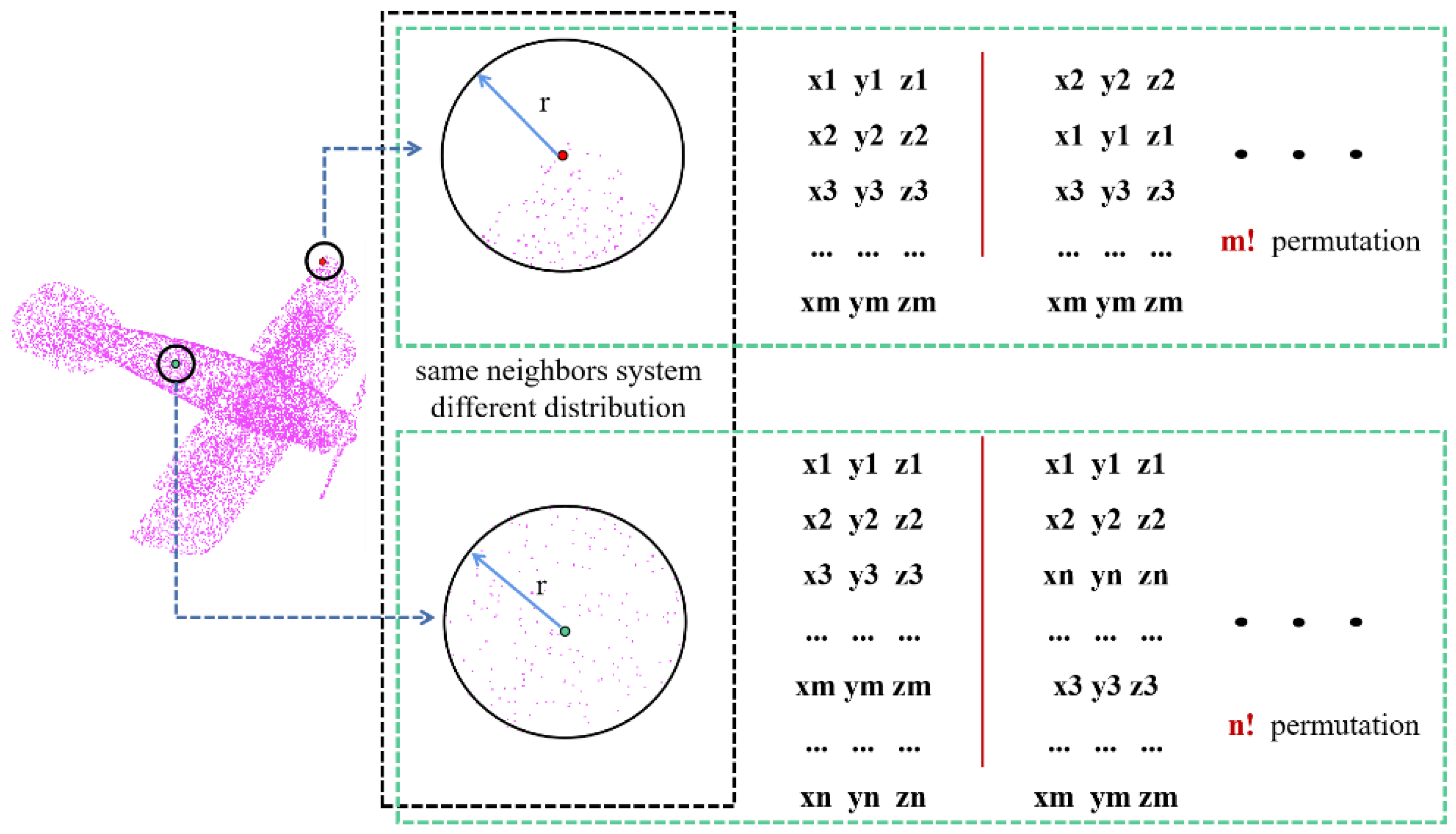
Let us look at the case of point clouds. Figure 3 illustrates the irregularity and disorder of a 3D point cloud. The left-hand side of Figure 3 represents the original point cloud of an object, for which we can identify a radius neighborhood system. The black dashed box in the middle indicates the irregularity of the point cloud, with different numbers of points and an uneven distribution within the same neighborhood. The green dashed box on the right-hand side reflects the disorder of the point cloud, with N being the number of point clouds, which can be seen to have N! permutations.

Figure 3. The irregularity and disorder of a 3D point cloud: The point cloud is shown on the left. The middle black dashed box shows the irregularity of the 3D point cloud with the same neighbor radius r, different numbers of points (m and n), and different distributions. The green dashed boxes on the right both show the disorder of the 3D point cloud, where the same point cloud has n! different orders, although they express the same entity.

When we want to apply standard convolution to a point cloud, the first problem is caused by its irregularity. The same neighborhood system has different numbers of points in different areas, meaning that we cannot determine the size of the convolution kernel. Now, let us suppose that by some sampling method, we obtain the same number of points in the neighborhood. It is then possible to determine the convolution kernel size as the number of points with a certain neighborhood size whose different convolution kernel element positions will have different parameters. The second problem is caused by its disorder, as the same point clouds have different N! permutations. In Figure 4, (x1, y1, z1) are the point coordinates, a is the kernel point without correspondence, and C(a) is the kernel point with correspondence. On the left of Figure 4, for the element b in the kernel, the point (x2, y2, z2) in the original sequence indicates b according to the default correspondence. When the point cloud is shuffled according to another arrangement, the point (x2, y2, z2) indicates d, while the point (xm, ym, zm) indicates b. This must result in a different value from what was obtained earlier after multiplying and summing the operations. Using a deterministic convolution kernel and according to standard convolution, we will obtain N! different convolution values, which is not the result that we want. Even if we have N! permutations, after a convolution operation, we always want to obtain the same result. Figure 4 describes the convolution operation for the shuffled points.

Figure 4. The convolution operation for the shuffled points with and without correspondences: (x1, y1, z1) are the point coordinates, a is the kernel point without correspondence, and C(a) is the kernel point with correspondence. The left-hand panel shows that the convolution without correspondences after shuffling will cause a different result. The right-hand panel shows that for the convolution operation with correspondences after the points have been shuffled, the shuffled points always indicate the same parameter, and the result is unchanged.

To maintain consistent convolution values, we need to keep the correspondence between the elements in the convolution range and the elements in the convolution kernel constant. In the right-hand panel of Figure 4, f(1) indicates a correspondence relationship between the first element in the kernel and the points. Once this correspondence has been established, the point (x2, y2, z2) always indicates b, even if the order is shuffled. All of this is necessary is to find correspondences in the point clouds and, thus, resolve the disorder problem.

Let us now return to the problem of irregularity.

We can take an image as an example to analyze the different types of correspondence between the convolution range and the convolution kernel (Figure 5). In order to later expand the principle to point clouds, we can rearrange the image by column and by the pixel index position. The upper panel in the figure is the original image; the bottom panel is the reorganized image. In the left-hand panel of the figure, N-to-N represents the standard image convolution, where different positions have different parameter values. If all values are the same within the convolution kernel, this is equivalent to a single identical value, which can be seen as an N-to-1 correspondence. Figure 4 shows the correspondence types. Due to the irregularity, we need to use N-to-M correspondence for processing the point cloud. At this point, the irregularity of the point clouds is also solved.

Figure 5. The types of correspondence for discrete convolution: N-to-N correspondence describes the standard image convolution; N-to-1 is used if the parameters are the same in all locations. The black circle is the convolution operation, the arrow are the correspondence. There are other correspondence types, e.g., N-to-M, etc.

In summary, the discrete convolution formula is reformulated as follows:

$$(f\ast g)(k)={\displaystyle \sum _{i=0}^I{\displaystyle \sum _{j=0}^j\stackrel{\psi (i,j)=C}{\underset{i\in N(k)}{f(i)}*\underset{j\in \mathrm{kernel}}{g(j)}}}},$$

(3)

where $k$ is the convolution element under consideration, $i\in N(k)$ means that $i$ is a neighboring point of $k$ in a neighbor system, $j$ is an element belonging to the convolution kernel, and $\psi (i,j)=C$ indicates that $i$ and $j$ should satisfy a constraint—also called the correspondence relationship.

The $k$ in Formula (3) can represent not only 1D data, but also 2D and higher-dimensional data. When $k$ represents 1D data, the correspondence relationship $\psi (i,j)=C$ satisfies $i+j=n$ and, thus, Formula (3) can be used for one-dimensional discrete convolution, similar to Formula (1). When $k$ represents 2D data, such as an image $(s,t)$, in this case, $i$ is $(m,n)$ and $j$ is $(p,q)$; therefore, the correspondence relationship $\psi (i,j)=C$ satisfies $[m+p=s,n+q=t]$, as described by Formula (2). When $k$ represents a 3D point cloud, which can be represented as $(x,y,z)$, $i$ is $(l,m,n)$ and $j$ is $(r,s,t)$. We thus need to find $\psi (i,j)=C$ for a point cloud.

3.2. Spatial Location Correspondence

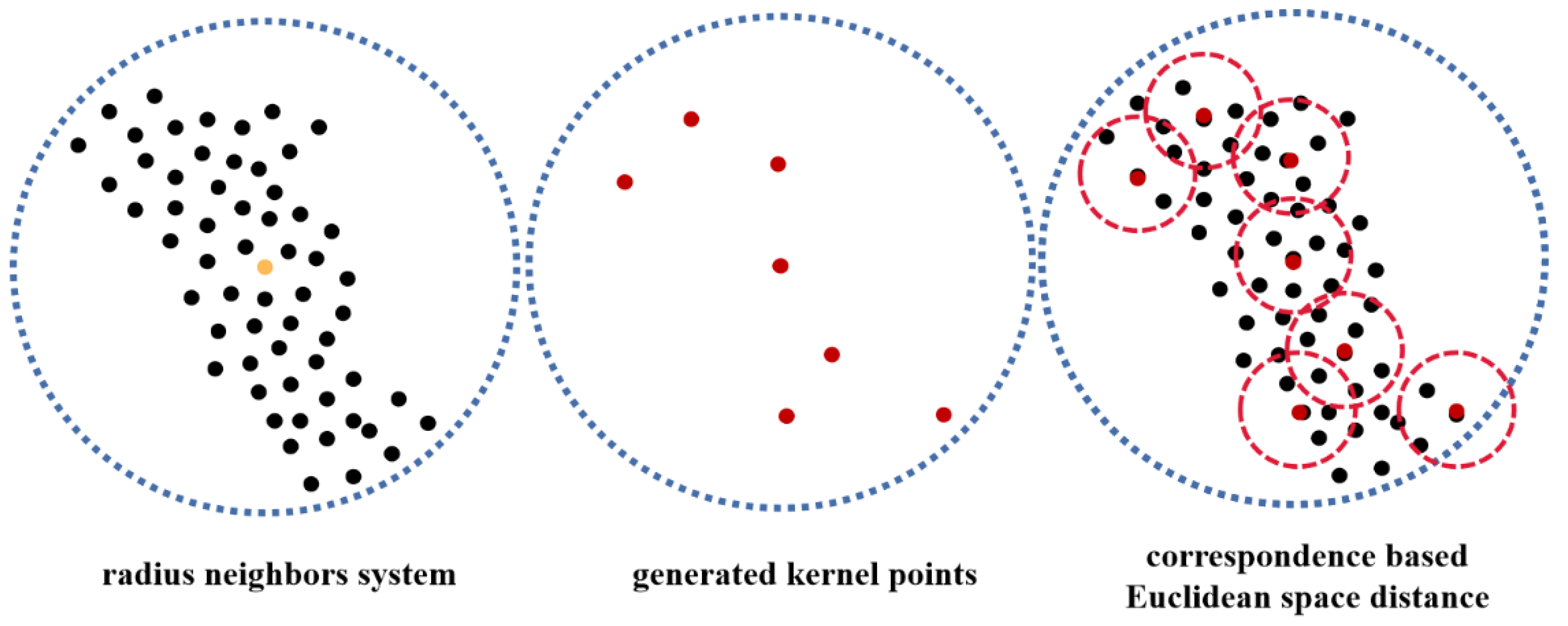
In light of this understanding of point clouds, we used the spatial positional correspondences as spatial data. Correspondences based on the Euclidean spatial location can be used to establish the correspondences of point clouds. We can assign the spatial coordinate points of the elements within the convolution kernel, which can be generated by different functions. The neighbors of the convolution kernel points are determined in the convolution range, which means that points in the convolution range will always have an unchanged correspondence. The points within the neighbors of a convolution kernel point will satisfy this correspondence. No matter how their order of permutation changes, this neighbor’s correspondence never changes, so the final convolution value remains constant. This correspondence based on the Euclidean spatial location can solve the problem of disorder in 3D point clouds and, in combination with the N-to-M correspondence strategy, can also solve the irregularity of 3D point clouds. Therefore, we can generalize the convolution operation and apply it to point clouds. Figure 6 describes the correspondences based on Euclidean spatial locations in 3D point clouds, represented by circles for convenience.

Figure 6. The correspondences based on Euclidean spatial locations in 3D point clouds. The left-hand circle shows the convolution range in a radius neighbor system, where the orange point is the convolution point and the points in the blue dotted circle are its neighbors. The middle circle shows the convolution kernel points generated by a certain function; these points will have 3D spatial coordinates. The right-hand circle describes the correspondence relationships based on the Euclidean spatial location.

3.3. Point Convolution Framework

On the basis of the discussion above, we can establish a general convolution framework that can be applied to point clouds. Figure 1 describes a general convolution framework for point clouds.

For 3D point clouds, we can identify a specific point cloud convolution operation according to the proposed framework via the following steps:

(1)

First, determine a suitable point cloud neighborhood system.

(2)

Second, determine how the convolution kernel’s coordinate points are generated and the appropriate size of the convolution kernel. In this study, we generated the kernel points from the covariance matrix of a sample.

(3)

Third, determine the range of influence of each of the convolution kernel points based on the Euclidean spatial location.

(4)

Finally, apply the convolution operation according to the correspondence.

3.4. An Example of a Network

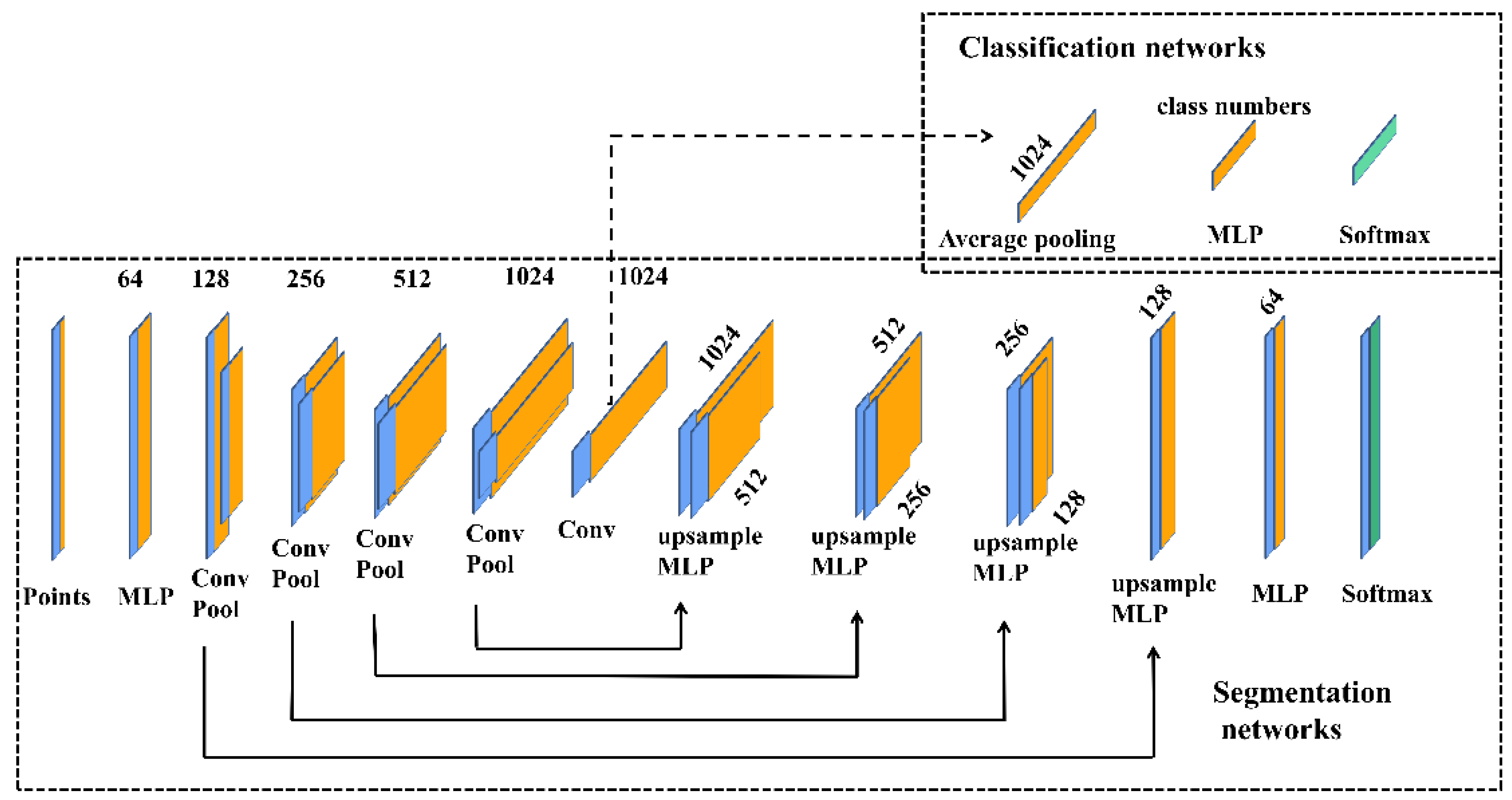
As an example of a convolution operation for point clouds based on the above analysis, we built a network using an encoder–decoder framework. We used the radius neighborhood. A previous study [30] has shown that the radius-based neighborhood system has a better representation in point clouds. We chose to generate the convolution kernel points according to the covariance matrix of the samples, where each layer had a different kernel according to the covariance matrix of the samples. Each layer used a ResNet architecture with grid sampling for pooling. The convolution and pooling modules both had a standard ResNet block. Figure 7 describes the convolution and pooling layers.

Figure 7. The convolution and pooling layers; the top panel is the convolution operation block.

The bottom panel is the pooling operation block. D_in and D_out represent the input feature dimensions and output feature dimensions in the current layer, respectively. In this study, we chose to generate the convolution kernel points according to the covariance matrix of the samples. Figure 8 describes the overall architecture of the network.

Figure 8. The overall architecture of the network: The backbone uses the encoder–decoder architecture and the skip connection. The upper branch shows the classification networks. The bottom branch shows the semantic segmentation networks.

4. Results and Discussion

We conducted mass experiments to validate our ideas, including classification and semantic segmentation tasks for 3D point clouds. All tasks were tested on an NVIDIA GPU Tesla V100 32GB. All experiments used the Adam optimizer. Our augmentation procedure consisted of scaling, flipping, and noising the points. The number of kernel points was 13 in all experiments unless otherwise noted.

4.1. Classification Tasks

ModelNet40 Classification

We tested our model on the ModelNet40 [31] classification task. The ModelNet40 dataset contains synthetic object point clouds. As the most widely used benchmark for point cloud analysis, ModelNet40 is popular because of its various categories, clean shapes, well-constructed dataset, etc. The original ModelNet40 dataset consists of 12,311 CAD-generated meshes in 40 categories (such as airplanes, cars, plants, and lamps), of which 9843 were used for training, while the other 2468 were reserved for testing. The corresponding point cloud data points were uniformly sampled from the mesh surfaces and then preprocessed by moving to the origin and scaling into a unit sphere.

We followed standard training/testing splits and rescaled the objects to fit them into a unit sphere. We ignored normals, as only artificial data were available. The first sample size was 0.02 m, and each subsequent layer was sampled at two times the size of the previous layer. The convolution kernel radius was the sample size of the current layer multiplied by the density parameter, which was a constant number that we set to 5. The batch size was 32 and the learning rate was 0.001. The momentum for batch normalization was 0.98.

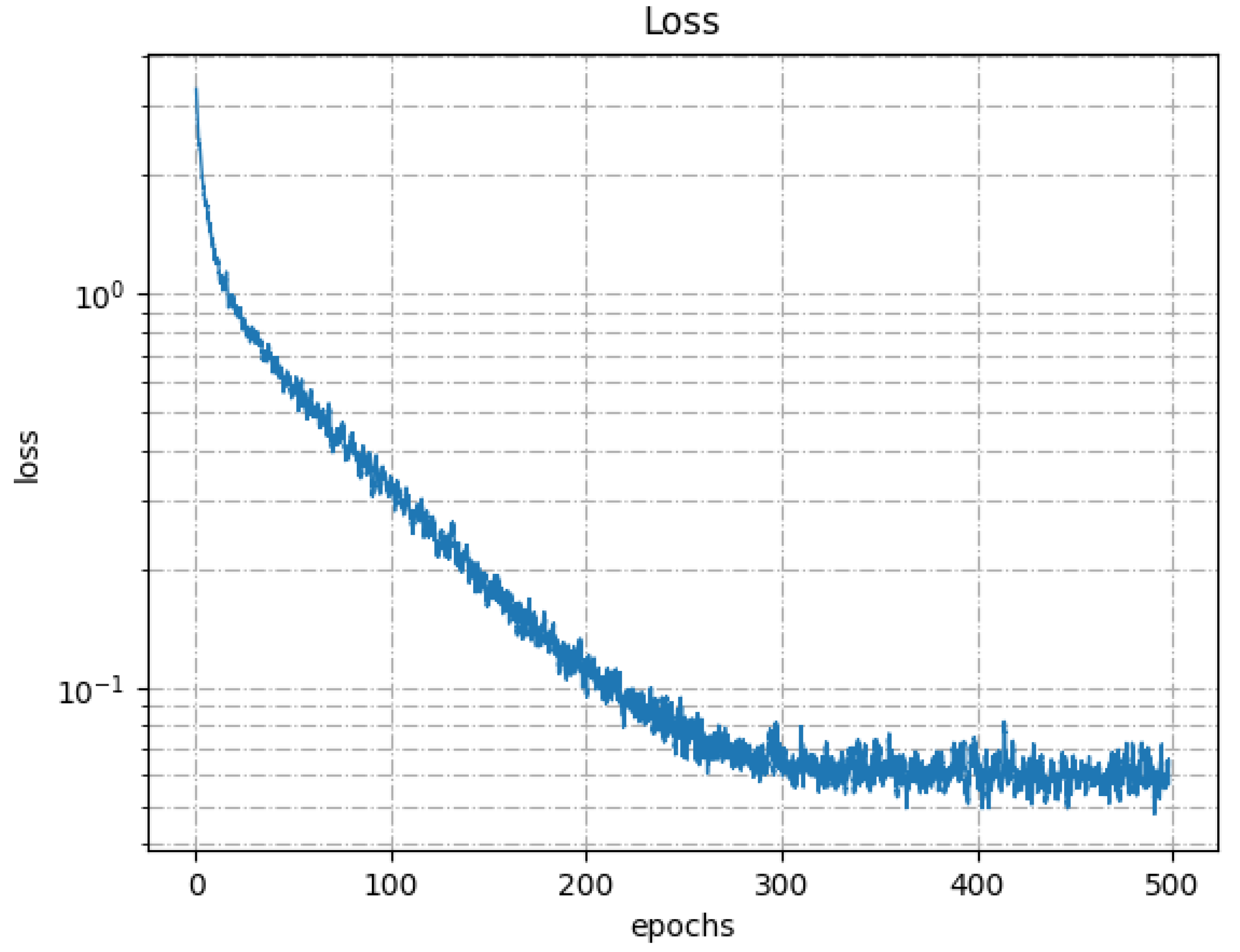
Table 1 shows the 3D shape classification results. The networks shown in the table include the currently existing 3D point cloud classification networks. Our covariance model achieved 92.7% overall accuracy—up to 3.5% more than PointNet [17], and 0.2% less than KPConv [8], which had the best result, as shown in Table 1. This covariance method allowed us to better fit the distribution of the data and learn more targeted features. Figure 9 shows the loss curve.

Table 1. Results for 3D shape classification: The metric is the overall accuracy (OA) for the ModelNet40 data. Ours—Covariance refers to the kernel points generated by the covariance matrix of the samples; Ours—Random randomly generated the kernel points.

Networks	Modelnet40
	OA (%)
PointNet [17]	89.2
PointNet++ [18]	90.7
SO-Net [32]	90.9
SpiderCNN [33]	90.5
FlexConv [24]	90.2
DGCNN [7]	92.2
SPH3D [27]	92.1
PointConv [26]	92.5
KPConv [8]	92.9
Ours—Covariance	92.7
Ours—Random	91.5

Figure 9. The loss curve for ModelNet40 classification.

4.2. Semantic Segmentation Tasks

Semantic segmentation was tested using three datasets: S3IDS [1], Semantic3D [2], and SensatUrban [3].

4.2.1. S3DIS: Semantic Segmentation for Indoor Scenes

We evaluated our model on the S3DIS dataset for a semantic scene segmentation task. This dataset includes 3D scanning point clouds for six indoor areas, including 272 rooms in total. Each point belongs to 1 of 13 semantic categories (e.g., board, bookcase, chair, ceiling, beam, etc.) plus clutter.

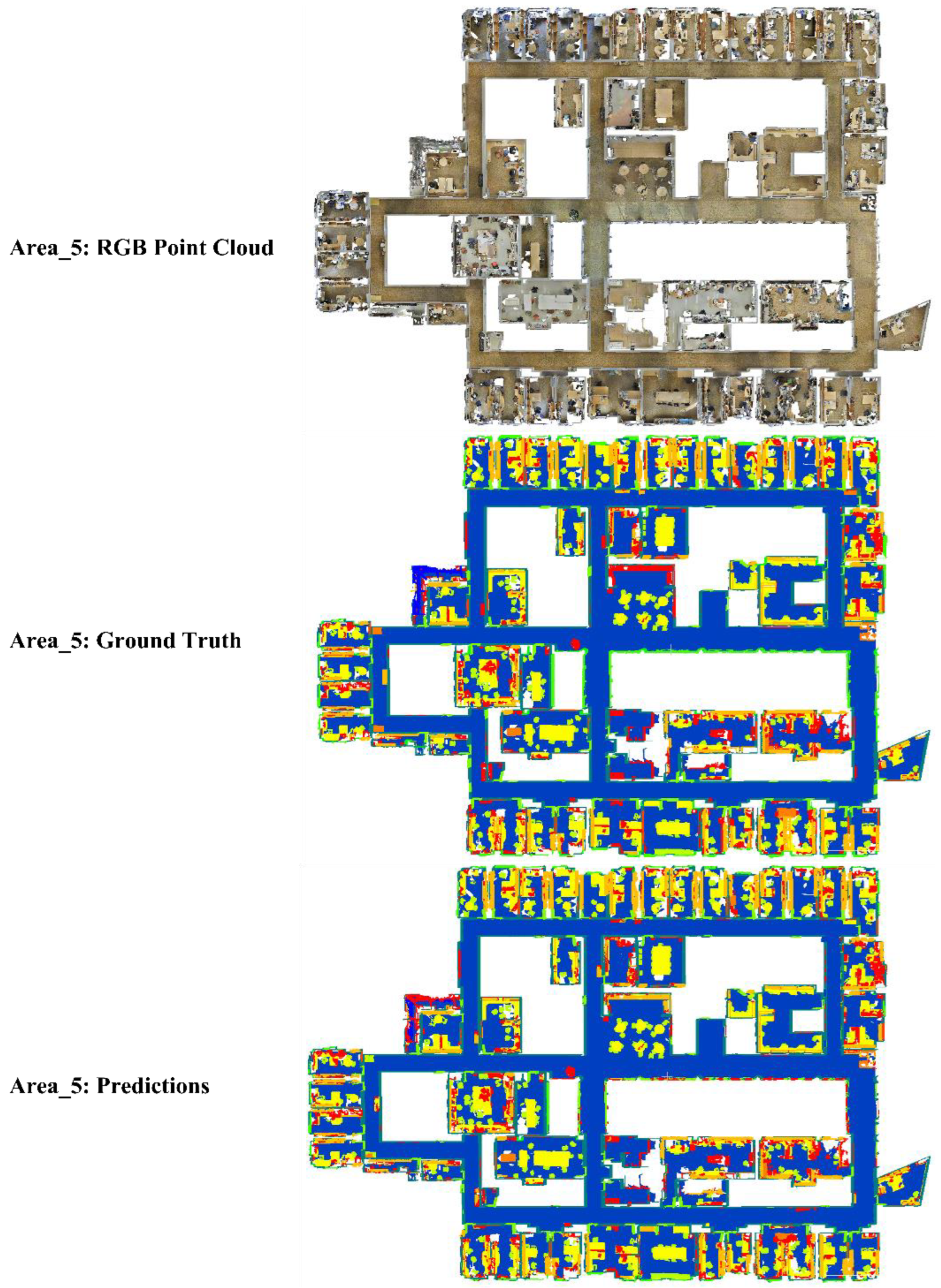
In the experiment, each point was represented as a 9D vector (XYZ, RGB, and normalized spatial coordinates). The training areas were Areas 1, 2, 3, 4, and 6, and the test area was Area 5. The input radius sample was 1 m. The first sample size was 0.04 m, and each subsequent layer was sampled at two times the size of the previous layer. The convolution kernel radius was the sample size of the current layer multiplied by the density parameter, which was a constant number that we set to 5. The batch size was 12, and the learning rate was 0.01. The momentum for batch normalization was 0.98. We generated the kernel points using the covariance matrix of the samples. Figure 10 shows the semantic segmentation results for Area 5.

Figure 10. The semantic segmentation results of Area 5: The top panel shows the raw RGB data. The middle panel is the ground truth. The bottom panel shows the predictions.

Table 2 describes the metrics compared with other networks. Our model achieves the best mIOU (64.6%) and mean class accuracy (69.6%) compared with the other models shown in the table, except for being only slightly lower than KPConv [8].

Table 2. Semantic segmentation mIoU scores for S3DIS Area 5.

Method	mIOU	Acc	Ceil.	Floor	Wall	Beam	Col.	Win.	Door	Table	Chair	Book.	Sofa	Broad	Clut.
PointNet [17]	41.1	49.0	88.8	97.3	69.8	0.1	3.9	46.3	10.8	58.9	52.6	58.9	40.3	5.9	26.4
SEGCloud [34]	48.9	57.4	90.1	96.1	69.9	0.0	18.4	38.4	23.1	70.4	75.9	70.4	58.4	40.9	13.0
Tanentconv [12]	52.6	62.2	90.5	97.7	74.0	0.0	20.7	39.0	31.3	77.5	69.4	77.5	38.5	57.3	48.8
SPGraph [20]	58.0	66.5	89.4	96.9	78.1	0.0	42.8	48.9	61.6	75.4	84.7	75.4	69.8	52.6	2.1
Paramconv [13]	58.3	67.1	92.3	96.2	75.9	0.3	6.0	69.5	63.5	65.6	66.9	65.6	47.3	68.9	59.1
SPH3d [27]	59.5	-	93.3	97.1	81.1	0.0	33.2	45.8	43.8	79.7	86.9	71.5	33.2	54.1	53.7
KPConv [8]	65.4	70.9	92.6	97.3	81.4	0.0	16.5	54.5	69.5	80.2	90.1	80.2	74.6	66.4	63.7
Ours	64.6	69.6	93.0	97.4	82.3	0.2	29.3	60.3	62.1	78.6	89.1	78.3	75.2	67.2	26.8

4.2.2. Semantic3D: LiDAR Semantic Segmentation

Semantic3D [2] is a point cloud dataset of scanned outdoor scenes with over 3 billion points. It contains 15 training and 15 test scenes annotated as eight classes. This large, natural, labeled 3D point cloud dataset covers a range of diverse urban scenes, including churches, streets, railroad tracks, and squares.

To examine the performance of our network on LiDAR data without color information, we trained two models with this dataset: one with colored LiDAR data, represented as XYZRGB; and one without colored data, which only represented XYZ. For some unknown reason, the Semantic3D benchmark [35] has not been able to evaluate the test set for some time, and we could only provide visual results of the test set. However, we provided visualization and evaluation of the validation set, and the split of the validation datasets followed KPConv [8].

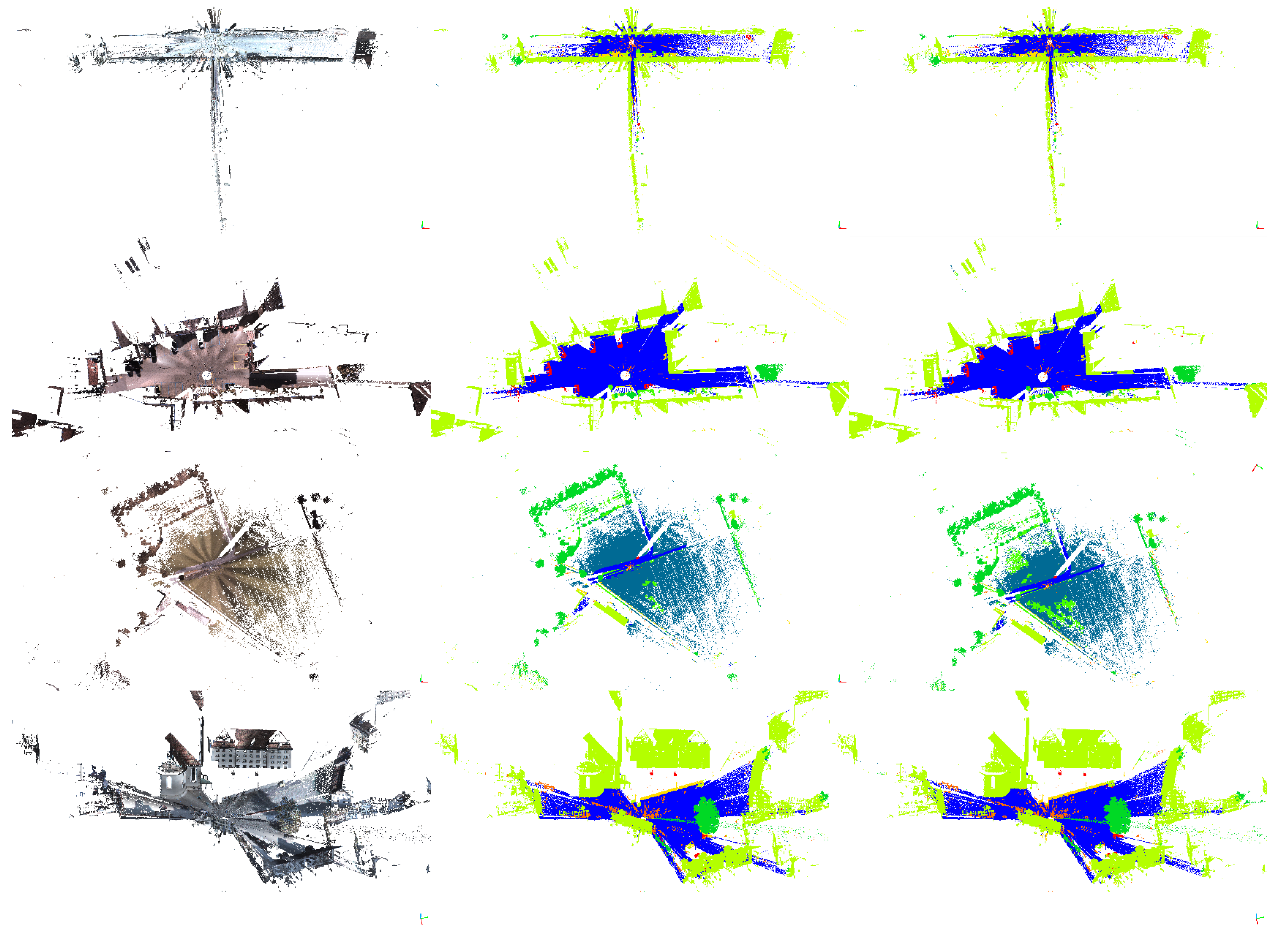
In the with-color experiment, each point was represented as a 9D vector (XYZ, RGB, and normalized spatial coordinates). In the without-color experiment, each point was represented as a 6D vector (XYZ and normalized spatial coordinates), and the other parameter were the same. The training dataset we used included the officially provided data; we used the reduced-8 data for testing. The input radius sample was 3 m. The first sample size was 0.06 m, and each subsequent layer was sampled at two times the size of the previous layer. The convolution kernel radius was the sample size of the current layer multiplied by the density parameter, which was a constant number that we set to 5. The batch size was 16 and the learning rate was 0.01. The momentum for batch normalization was 0.98. We generated the kernel points using the covariance matrix of the samples. Figure 11 shows the semantic segmentation results for the reduced-8 data with/without color. According to the visualization results, there was little difference between the color model and the non-color model. Our analysis found that the objects of the scene were buildings, streets, vehicles, etc. These objects can be identified geometrically even if they have no color information.

Figure 11. The semantic segmentation results for the reduced-8 data: The left column shows the original data. The middle column shows the predicted results with color. The right column shows the predicted results without color.

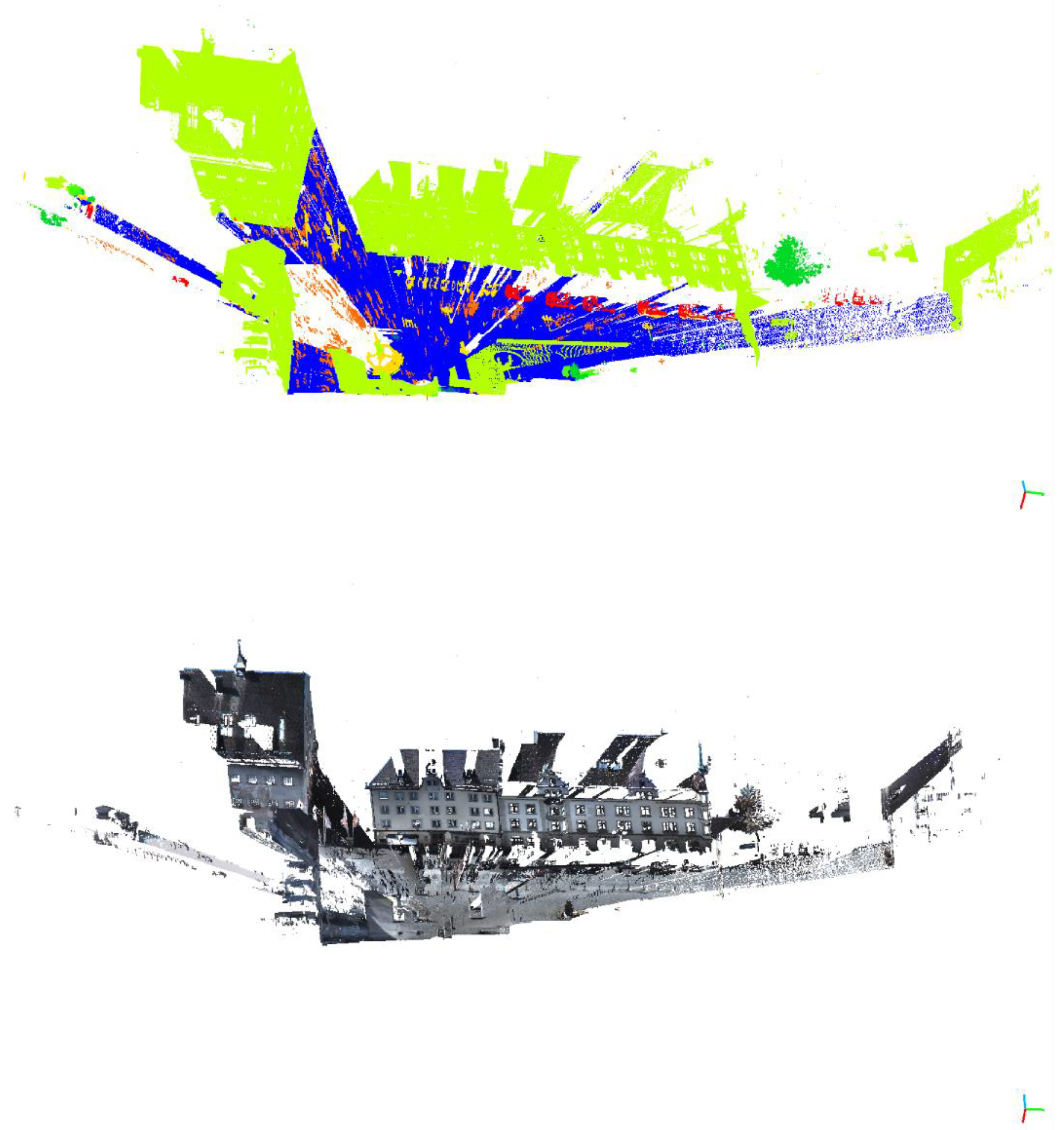
Table 3 describes the details of the metrics compared with other networks on reduced-8 with the colored model. Our model achieved an mIOU of 75.5%, and the natural scenes and cars achieved the best class accuracy. Since the Semantic3D benchmark [35] cannot currently provide the results of the test set for unknown reasons, we could not provide the metric evaluation of the non-colored model, but we provided the visualization and metric evaluation results of the validation set, as shown in Figure 12 and Table 4, respectively.

Table 3. Semantic segmentation results for reduced-8 data.

Method	mIOU	OA	Man.	Natural.	High Veg.	Low Veg.	Building	Hard.	Scan.	Cars
SEGCloud [34]	59.1	88.6	82.0	77.3	79.7	22.9	91.1	18.4	37.3	64.4
SPGraph [20]	73.0	84.0	97.4	92.6	87.9	44.0	83.2	31.0	63.5	76.2
KPConv [8]	74.6	92.9	90.9	82.2	84.2	47.9	94.9	40.0	77.3	79.7
RandLA-NET [15]	77.4	94.8	95.6	91.4	86.6	51.5	95.7	51.5	69.8	76.8
Ours—colored	74.4	92.7	90.5	90.7	82.6	46.5	90.6	50.6	70.3	73.7

Figure 12. The semantic segmentation results for the validation data: The top panel shows the original data. The bottom panel is the predicted result.

Table 4. Semantic segmentation results for the validation data.

Model	mIOU	OA	Man.	Natural.	High Veg.	Low veg.	Building	Hard.	Scan.	Cars
Non-colored	79.0	95.9	97.7	78..8	77.3	35.7	98.9	70.3	74.2	99.2

4.2.3. SensatUrban: Photogrammetric Point Cloud Datasets at the City Level

The SensatUrban [3] dataset is an urban-scale photogrammetric point cloud dataset with nearly 3 billion richly annotated points. The dataset consists of large areas from two UK cities, covering about 6 km² of the city landscape. In the dataset, each 3D point is labeled as one of 13 semantic classes (e.g., ground, vegetation, cars, etc.).

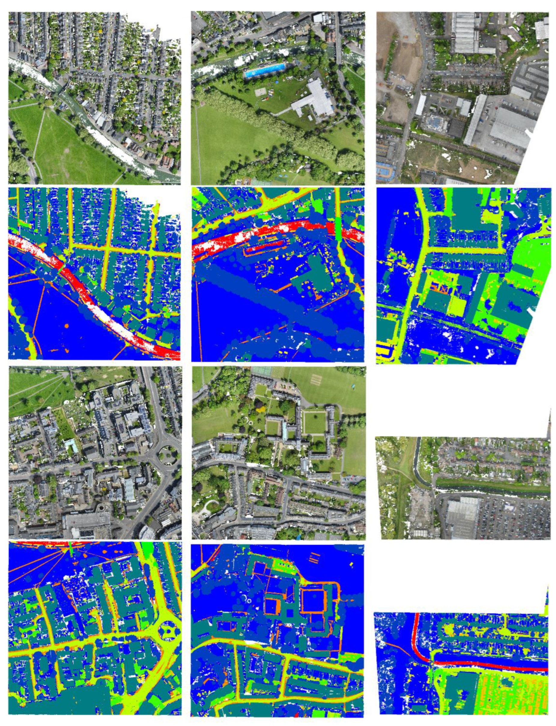
In the experiment, each point was represented as a 9D vector (XYZ, RGB, and normalized spatial coordinates). The training and testing datasets that we used were consistent with those of SensatUrban [3]. The input radius sample was 5 m. The first sample size was 0.1 m, and each subsequent layer was sampled at two times the size of the previous layer. The convolution kernel radius was the sample size of the current layer multiplied by the density parameter, which was a constant number that we set to 5. The batch size was 16 and the learning rate was 0.01. The momentum for batch normalization was 0.98. We generated the kernel points using the covariance matrix of the samples. Figure 13 shows the semantic segmentation results for SensatUrban.

Figure 13. Semantic segmentation results for SensatUrban: The first and third rows show the original data. The second and fourth rows show the predicted results.

Table 5 describes the detailed semantic segmentation metrics for SensatUrban. Our model achieved an mIOU of 56.92%.

Table 5. Semantic segmentation results for SensatUrban.

Method	OA	mIOU	Grou.	Veg.	Buil.	Wall	Brid.	Park.	Rail	Traf.	Stre.	Car	Foo.	Bike	Water
PointNet [17]	80.78	23.71	67.96	89.52	80.05	0.00	0.00	3.95	0.00	31.55	0.00	35.14	0.00	0.00	0.00
PointNet++ [18]	84.30	32.92	72.46	94.24	84.77	2.72	2.09	25.79	0.00	31.54	11.42	38.84	7.12	0.00	56.93
SPGraph [20]	85.27	37.29	69.93	94.55	88.87	32.83	12.58	15.77	15.48	30.63	22.96	56.42	0.54	0.00	44.24
SparseConv [16]	88.66	42.66	74.10	97.90	94.20	63.30	7.50	24.20	0.00	30.10	34.00	74.40	0.00	0.00	54.80
KPConv [8]	93.20	57.58	87.10	98.91	95.33	74.40	28.69	41.38	0.00	55.99	54.43	85.67	40.39	0.00	86.30
RandLA-Net [15]	89.78	52.69	80.11	98.07	91.58	48.88	40.75	51.62	0.00	56.67	33.23	80.14	32.63	0.00	71.31
Ours	91.6	56.92	86.56	98.08	92.35	68.6	35.68	49.56	5.63	57.86	40.36	86.25	38.36	0.00	80.63

4.3. Discussion

We chose two key factors to test their impact on the results: the way in which the kernel points were generated, and the number of kernel points.

4.3.1. The Way in Which the Kernel Points Were Generated

We compared the classification effects of different kernel generation methods, namely, the covariance matrix of samples and the random method. The former generates the kernel points according to the covariance matrix of samples; the latter generates the kernel points from random points in a unit sphere.

In Table 1, we can see that even the random method had an accuracy of 91.5—2.3% higher than PointNet [17], and less than 1.2% lower compared with covariance—so we believe that the randomly generated kernel points may not match the data. This suggests that kernel points consistent with the data distribution may be learned for better expression. This encourages us to generate a convolution kernel point that fits the data more closely, which is a direction for our future work.

4.3.2. The Number of Kernel Points

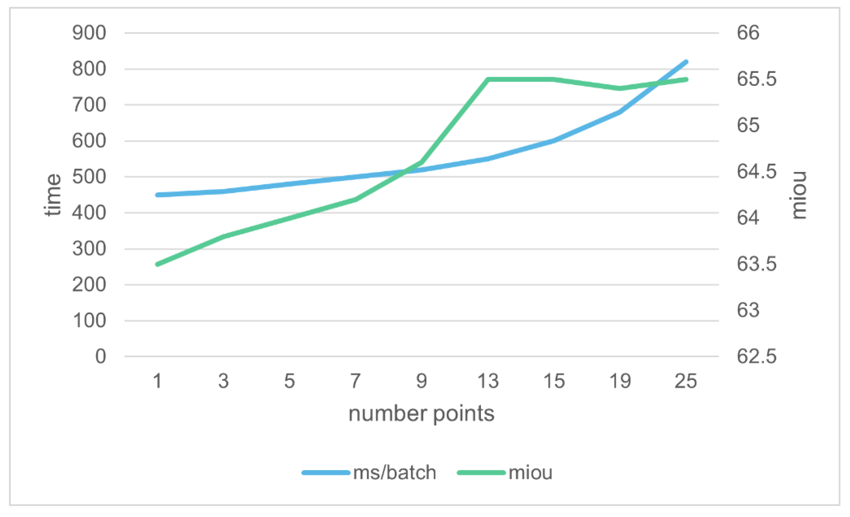
We conducted a comparison experiment on the effect and the time for different numbers of kernel points in a semantic segmentation task with the S3DIS dataset. The convolution kernel points were generated from the covariance matrix of the samples. Figure 14 shows the results.

Figure 14. mIOU and time of semantic segmentation for different numbers of kernel points.

As shown in Figure 12, the mIOU reached its maximum when the number of kernel points was 13, and it did not continue to improve beyond this number. The time kept increasing as the number of points increased, as expected. This tells us that if we pursue speed, then we should reduce the number of kernels, while if we pursue accuracy, then we need to increase the number of kernel points, which we need to balance according to our needs. It should be noted that the optimal number of convolution kernel points is not fixed, depending on the different datasets, the sampling density, the framework’s structure, and the number of layers.

5. Conclusions

In this work, we propose a convolution framework that can be directly applied to point clouds and considers the spatial position correspondences. We analyzed the mathematical nature of convolution and found that the convolution operation remains unchanged as long as the correspondences remain unchanged. Moreover, we discussed the types of correspondence relationships based on the location and the influence of the number and generation method of the kernel points. We validated our convolution network through classification and semantic segmentation tasks. Based on the results, our proposed spatial position correspondences are applicable to point clouds. This can be used as a principle to guide us in designing point cloud convolutional networks that meet our diverse needs. Combined with the framework, we only need to establish the individual steps to establish a deterministic network to achieve a fast or high-precision point cloud processing application. This helps us to focus on how to solve the whole problem instead of trying to design complex and incomprehensible network modules.

In this paper, we mainly focus on point clouds with color. However, as we all know, not all point clouds have color—for example, Lidar point clouds. Exploring the proposed convolution method on point clouds without color will be the focus of our next work. In the meantime, we believe that our framework can be generalized to more data types—not just point clouds or images—and also for the joint processing of images and point clouds, as long as we find a suitable correspondence.

References

1. Armeni, I.; Sener, O.; Zamir, A.R.; Jiang, H.; Brilakis, I.; Fischer, M.; Savarese, S. 3D Semantic Parsing of Large-Scale Indoor Spaces. In Proceedings of the 2016 IEEE Conference on Computer Vision and Pattern Recognition (CVPR), Las Vegas, NV, USA, 27–30 June 2016; IEEE: Las Vegas, NV, USA; pp. 1534–1543. [Google Scholar]
2. Hackel, T.; Savinov, N.; Ladicky, L.; Wegner, J.D.; Schindler, K.; Pollefeys, M. Semantic3D. Net: A New Large-Scale Point Cloud Classification Benchmark. arXiv 2017, arXiv:1704.03847. [Google Scholar]
3. Hu, Q.; Yang, B.; Khalid, S.; Xiao, W.; Trigoni, N.; Markham, A. Towards Semantic Segmentation of Urban-Scale 3D Point Clouds: A Dataset, Benchmarks and Challenges. In Proceedings of the 2021 IEEE/CVF Conference on Computer Vision and Pattern Recognition (CVPR), Nashville, TN, USA, 20–25 June 2021; IEEE: Nashville, TN, USA; pp. 4975–4985. [Google Scholar]
4. Artificial Intelligence Computing Leadership from NVIDIA. Available online: https://www.nvidia.com/en-us/ (accessed on 18 July 2022).
5. TensorFlow. Available online: https://tensorflow.google.cn/?hl=en (accessed on 18 July 2022).
6. PyTorch. Available online: https://pytorch.org/ (accessed on 18 July 2022).
7. Wang, Y. DGCNN: Learning Point Cloud Representations by Dynamic Graph CNN. Ph.D. Thesis, Massachusetts Institute of Technology, Cambridge, MA, USA, 2020. [Google Scholar]
8. Thomas, H.; Qi, C.R.; Deschaud, J.-E.; Marcotegui, B.; Goulette, F.; Guibas, L.J. KPConv: Flexible and Deformable Convolution for Point Clouds. In Proceedings of the IEEE/CVF International Conference on Computer Vision (ICCV), Seoul, Republic of Korea, 27 October–2 November 2019. [Google Scholar]
9. Maturana, D.; Scherer, S. VoxNet: A 3D Convolutional Neural Network for Real-Time Object Recognition. In Proceedings of the 2015 IEEE/RSJ International Conference on Intelligent Robots and Systems (IROS), Hamburg, Germany, 28 September–3 October 2015; pp. 922–928. [Google Scholar]
10. Li, Y.; Bu, R.; Sun, M.; Wu, W.; Di, X.; Chen, B. PointCNN: Convolution On X-Transformed Points. In Proceedings of the Advances in Neural Information Processing Systems, Vancouver, BC, Canada, 8–14 December 2019; Curran Associates, Inc.: Red Hook, NY, USA, 2018; Volume 31. [Google Scholar]
11. Hua, B.-S.; Tran, M.-K.; Yeung, S.-K. Pointwise Convolutional Neural Networks. In Proceedings of the 2018 IEEE/CVF Conference on Computer Vision and Pattern Recognition, Salt Lake City, UT, USA, 18–23 June 2018; IEEE: Salt Lake City, UT, USA; pp. 984–993. [Google Scholar]
12. Tatarchenko, M.; Park, J.; Koltun, V.; Zhou, Q.-Y. Tangent Convolutions for Dense Prediction in 3D. arXiv 2018, arXiv:1807.02443. [Google Scholar]
13. Wang, S.; Suo, S.; Ma, W.-C.; Pokrovsky, A.; Urtasun, R. Deep Parametric Continuous Convolutional Neural Networks. In Proceedings of the 2018 IEEE/CVF Conference on Computer Vision and Pattern Recognition, Salt Lake City, UT, USA, 18–23 June 2018; pp. 2589–2597. [Google Scholar]
14. Deuge, M.D.; Quadros, A.; Hung, C.; Douillard, B. Unsupervised Feature Learning for Classification of Outdoor 3D Scans. In Proceedings of the Australasian Conference on Robotics and Automation, Sydney, Australia, 2–4 December 2013. [Google Scholar]
15. Hu, Q.; Yang, B.; Xie, L.; Rosa, S.; Guo, Y.; Wang, Z.; Trigoni, N.; Markham, A. RandLA-Net: Efficient Semantic Segmentation of Large-Scale Point Clouds. In Proceedings of the IEEE/CVF Conference on Computer Vision and Pattern Recognition (CVPR), Seattle, WA, USA, 13–19 June 2020. [Google Scholar]
16. Graham, B.; Engelcke, M.; van der Maaten, L. 3D Semantic Segmentation with Submanifold Sparse Convolutional Networks. In Proceedings of the 2018 IEEE/CVF Conference on Computer Vision and Pattern Recognition, Salt Lake City, UT, USA, 18–23 June 2018; IEEE: Salt Lake City, UT, USA; pp. 9224–9232. [Google Scholar]
17. Qi, C.R.; Su, H.; Mo, K.; Guibas, L.J. PointNet: Deep Learning on Point Sets for 3D Classification and Segmentation. In Proceedings of the IEEE Conference on Computer Vision and Pattern Recognition (CVPR), Honolulu, HI, USA, 21–26 July 2017. [Google Scholar]
18. Qi, C.R.; Yi, L.; Su, H.; Guibas, L.J. PointNet++: Deep Hierarchical Feature Learning on Point Sets in a Metric Space. Adv. Neural Inf. Process. Syst. 2017, 30. [Google Scholar]
19. Simonovsky, M.; Komodakis, N. Dynamic Edge-Conditioned Filters in Convolutional Neural Networks on Graphs. In Proceedings of the 2017 IEEE Conference on Computer Vision and Pattern Recognition (CVPR), Honolulu, HI, USA, 21–26 July 2017; pp. 29–38. [Google Scholar]
20. Landrieu, L.; Simonovsky, M. Large-Scale Point Cloud Semantic Segmentation with Superpoint Graphs. In Proceedings of the 2018 IEEE/CVF Conference on Computer Vision and Pattern Recognition, Salt Lake City, UT, USA, 18–23 June 2018; pp. 4558–4567. [Google Scholar]
21. Guo, M.-H.; Cai, J.; Liu, Z.-N.; Mu, T.-J.; Martin, R.; Hu, S. PCT: Point Cloud Transformer. Undefined 2021, 7, 187–199. [Google Scholar] [CrossRef]
22. Zhao, H.; Jiang, L.; Jia, J.; Torr, P.; Koltun, V. Point Transformer. In Proceedings of the IEEE/CVF Conference on Computer Vision and Pattern Recognition (CVPR), Seattle, WA, USA, 13–19 June 2020. [Google Scholar]
23. Engel, N.; Belagiannis, V.; Dietmayer, K. Point Transformer. IEEE Access 2021, 9, 134826–134840. [Google Scholar] [CrossRef]
24. Groh, F.; Wieschollek, P.; Lensch, H.P.A. Flex-Convolution (Million-Scale Point-Cloud Learning Beyond Grid-Worlds). arXiv 2020, arXiv:1803.07289. [Google Scholar]
25. Lei, H.; Akhtar, N.; Mian, A. Octree Guided CNN With Spherical Kernels for 3D Point Clouds. In Proceedings of the 2019 IEEE/CVF Conference on Computer Vision and Pattern Recognition (CVPR), Long Beach, CA, USA, 15–20 June 2019; IEEE: Long Beach, CA, USA; pp. 9623–9632. [Google Scholar]
26. Wu, W.; Qi, Z.; Fuxin, L. PointConv: Deep Convolutional Networks on 3D Point Clouds. In Proceedings of the IEEE/CVF Conference on Computer Vision and Pattern Recognition (CVPR), Seattle, WA, USA, 13–19 June 2020. [Google Scholar]
27. Lei, H.; Akhtar, N.; Mian, A. Spherical Kernel for Efficient Graph Convolution on 3D Point Clouds. IEEE Trans. Pattern Anal. Mach. Intell. 2021, 43, 3664–3680. [Google Scholar] [CrossRef] [PubMed]
28. Su, H.; Maji, S.; Kalogerakis, E.; Learned-Miller, E. Multi-View Convolutional Neural Networks for 3D Shape Recognition. In Proceedings of the 2015 IEEE International Conference on Computer Vision (ICCV), Santiago, Chile, 7–13 December 2015; pp. 945–953. [Google Scholar]
29. Lin, Z.-H.; Huang, S.-Y.; Wang, Y.-C.F. Convolution in the Cloud: Learning Deformable Kernels in 3D Graph Convolution Networks for Point Cloud Analysis. In Proceedings of the 2020 IEEE/CVF Conference on Computer Vision and Pattern Recognition (CVPR), Seattle, WA, USA, 13–19 June 2020; pp. 1797–1806. [Google Scholar]
30. Thomas, H.; Goulette, F.; Deschaud, J.-E.; Marcotegui, B.; LeGall, Y. Semantic Classification of 3D Point Clouds with Multiscale Spherical Neighborhoods. In Proceedings of the 2018 International Conference on 3D Vision (3DV), Verona, Italy, 5–8 September 2018; pp. 390–398. [Google Scholar]
31. Wu, Z.; Song, S.; Khosla, A.; Yu, F.; Zhang, L.; Tang, X.; Xiao, J. 3D ShapeNets: A Deep Representation for Volumetric Shapes. In Proceedings of the 2015 IEEE Conference on Computer Vision and Pattern Recognition (CVPR), Boston, MA, USA, 7–12 June 2015; IEEE: Boston, MA, USA; pp. 1912–1920. [Google Scholar]
32. Li, J.; Chen, B.M.; Lee, G.H. SO-Net: Self-Organizing Network for Point Cloud Analysis. In Proceedings of the 2018 IEEE/CVF Conference on Computer Vision and Pattern Recognition, Salt Lake City, UT, USA, 18–23 June 2018; pp. 9397–9406. [Google Scholar]
33. Xu, Y.; Fan, T.; Xu, M.; Zeng, L.; Qiao, Y. SpiderCNN: Deep Learning on Point Sets with Parameterized Convolutional Filters. In Proceedings of the European Conference on Computer Vision (ECCV), Munich, Germany, 8–14 September 2018. [Google Scholar]
34. Tchapmi, L.; Choy, C.; Armeni, I.; Gwak, J.; Savarese, S. SEGCloud: Semantic Segmentation of 3D Point Clouds. In Proceedings of the 2017 International Conference on 3D Vision (3DV), Qingdao, China, 10–12 October 2017; pp. 537–547. [Google Scholar]
35. Semantic3D. Available online: http://semantic3d.net/ (accessed on 16 November 2022).
Publisher’s Note: MDPI stays neutral with regard to jurisdictional claims in published maps and institutional affiliations.
Article Metrics
Citations
Article Access Statistics
Multiple requests from the same IP address are counted as one view.