Measuring the Similarity of Metro Stations Based on the Passenger Visit Distribution

Abstract

The distribution of passengers reflects the characteristics of urban rail stations. The automatic fare collection system of rail transit collects a large amount of passenger trajectory data tracking the entry and exit continuously, which provides a basis for detailed passenger distributions. We first exploit the Automatic Fare Collection (AFC) data to construct the passenger visit pattern distribution for stations. Then we measure the similarity of all stations using Wasserstein distance. Different from other similarity metrics, Wasserstein distance takes the similarity between values of quantitative variables in the one-dimensional distribution into consideration and can reflect the correlation between different dimensions of high-dimensional data. Even though the computational complexity grows, it is applicable in the metro stations since the scale of urban rail transit stations is limited to tens to hundreds and detailed modeling of the stations can be performed offline. Therefore, this paper proposes an integrated method that can cluster multi-dimensional joint distribution considering similarity and correlation. Then this method is applied to cluster the rail transit stations by the passenger visit distribution, which provides some valuable insight into the flow management and the station replanning of urban rail transit in the future.

1. Introduction

Urban rail transit is known for its fast speed, large capacity, high level of comfort, efficiency, and reliability. Effective operation of urban rail transit can reduce travel costs, transport more passengers, and relieve road traffic congestions. The urban rail transit system of various cities in China is developing rapidly and is serving more passengers. For example, the Beijing metro served 1846.3 million passengers in 2010, increasing by 114.6% to as high as 3962.3 million passengers in 2019 [1]. Making management policies to improve the system efficiency and reliability [2] requires a refined grasp of the characteristics of passengers at each station and each time period. Better management measures can improve the level of service and make rail transit play the role better as the backbone of the urban public transportation system in cities like Beijing [3].

The research on passenger characteristics can be divided into individual models and collective ones. The focus of individual research is from the perspective of individual passengers, and collective research analyzed is at the level of stations, routes, and networks with aggregated data [4]. With the increasing popularity of smart card data, research on transit passenger characteristics based on large-scale trajectory data continues to emerge [5,6]. Efforts are devoted to the individual passenger’s mode of commuting patterns [7,8], travel purpose inference [9], spatial patterns [10], temporal patterns [11,12], and spatial-temporal joint patterns [13,14]. One of the most commonly used methods is to cluster the travel patterns of passengers to better interpret their characteristics [15,16]. Collective passenger patterns analysis based on aggregated data focuses on understanding the usage frequency of stations [12], recognizing passenger gathering places [17], and identifying the spatial distribution of urban functional zones [18].

This article focuses on the passenger distribution aggregated at the station level. For the rail transit system, from the perspective of stations, the number of stations is limited. In China, as of 31 December 2020 [19], the Beijing Metro has the most operating stations at 428, followed by the Shanghai Metro with 354. The size of the stations reduces the scale of the problem to understand the characteristics of the stations better. Therefore, rail transit station managers and operators do not need to consider handling large-scale datasets like other machine learning practitioners. At the same time, a more accurate understanding could lead to better travel flow management and control measures. Instead of focusing on efficiency, more efforts should be taken to make full use of the behaviors of all passengers related to the station when investigating a certain station. Passengers can be represented as a random variable, which is often described by statistical representative values such as the total inflow/outflow [20] or mean for quantitative variables [21]. These methods are straightforward and have the advantage in applicability and scalability. However, passenger distributions contain a lot more information than one single representative value. This article fills the gap by measuring the similarity of distributions rather than using a simple representative value such as median or average. We aim to take full advantage of distributions for the stations at a small scale, rather than replace other methods completely in any case.

The idea of this paper is similar to decomposing high-dimensional tensors or tensors with time series by adding a temporal smoothing term [22], or spatial regularization term according to the topology and spatial proximity [23], and to consider the spatio-temporal correlation between data points. Temporal smoothing terms constrain the adjacent or periodical time to be close [24], and spatial regularization terms minimize the gap for points with similar geographic attributes. Different from considering different data points of the same attribute in the above research, this paper assumes the correlation between different values of the same attribute at the same data point.

We utilize the proposed method to cluster stations by their passenger visit distribution. The grasp of passenger visit distribution plays a role in station facilities planning such as map [25] or route guide signs setting [26], flow management under both normal [27] and emergency conditions [28], and business commercial advertisement design [29].

The first significance of passenger visit distribution lies in the route guide signs settings [26,30]. For example, for stations such as Airport Terminal T2, almost all passengers only visit once or twice. These passengers are not familiar with the internal structure and proper route in the station, so it should intensively display guide signs leading to the platform and different exits without other interference for both passengers entering and leaving the station. On the contrary, if all passengers visit a certain station frequently, they are familiar with the station. The real-time information of trains and passenger flow can be displayed for the inbound passengers, and richer information about the exit and even more commercial advertisements can be displayed for the outbound passengers. To sum up, the sign display strategy should be adjusted according to the passengers’ familiarity with the stations.

The second potential use lies in the passenger flow control within the station. The route choice behavior is also dependent on the familiarity of passengers with the stations, streamline of the stations for passenger flow management [31]. For stations with different passengers’ familiarity distributions, different control methods should be exploited to make sure passengers obey the rules since familiar passengers show different preferences when choosing routes [32]. Passengers unfamiliar with the stations could fail to find the shortest path under emergency evacuation. Thus, when evaluating the emergency evacuation efficiency, the passenger visit distribution should be considered.

The third opportunity the passenger visit distribution provides is to improve the business commercial advertisement [29] displayed in the metro stations. The stations of familiar passengers with repeated visited patterns are of preference for those advertisements targeted to show repeatedly to the same passengers. Railway stations and Airport terminals attracting different unfamiliar passengers are suitable for commercials wishing to cover as most passengers as possible.

The goal of this research is to first construct the visit count distribution, then measure the similarity of all stations using Wasserstein distance and cluster the stations according to the visit distribution similarity matrix for policy implications. The main contributions of this paper are threefold. First, we use Wasserstein distance to measure the similarity, taking into account the similar visit count. By customizing the cost function, the correlation between station-specific visit count and total visit count can be considered. This is also applicable for multi-dimensional joint distribution with multiple attributes, or the time series of multi-dimensional attributes. Second, the obtained distance matrix is used to cluster stations according to the passenger visit distribution of stations, demonstrating its practicability and effectiveness. Lastly, the case study of passenger familiarity clustering for Beijing metro stations further quantitatively characterizes the Beijing metro stations, providing insights for the refined flow management of urban rail transit passengers.

The remainder of the paper is organized as follows. The study area, the Automatic Fare Collection (AFC) data, similarity measures, and the clustering method are presented in Section 2. Section 3 shows how we construct the visit distribution, measure the similarity and cluster the stations, together with the analysis of the clustering results. Section 4 concludes the paper and discusses the implications of the results.

2. Materials and Methods

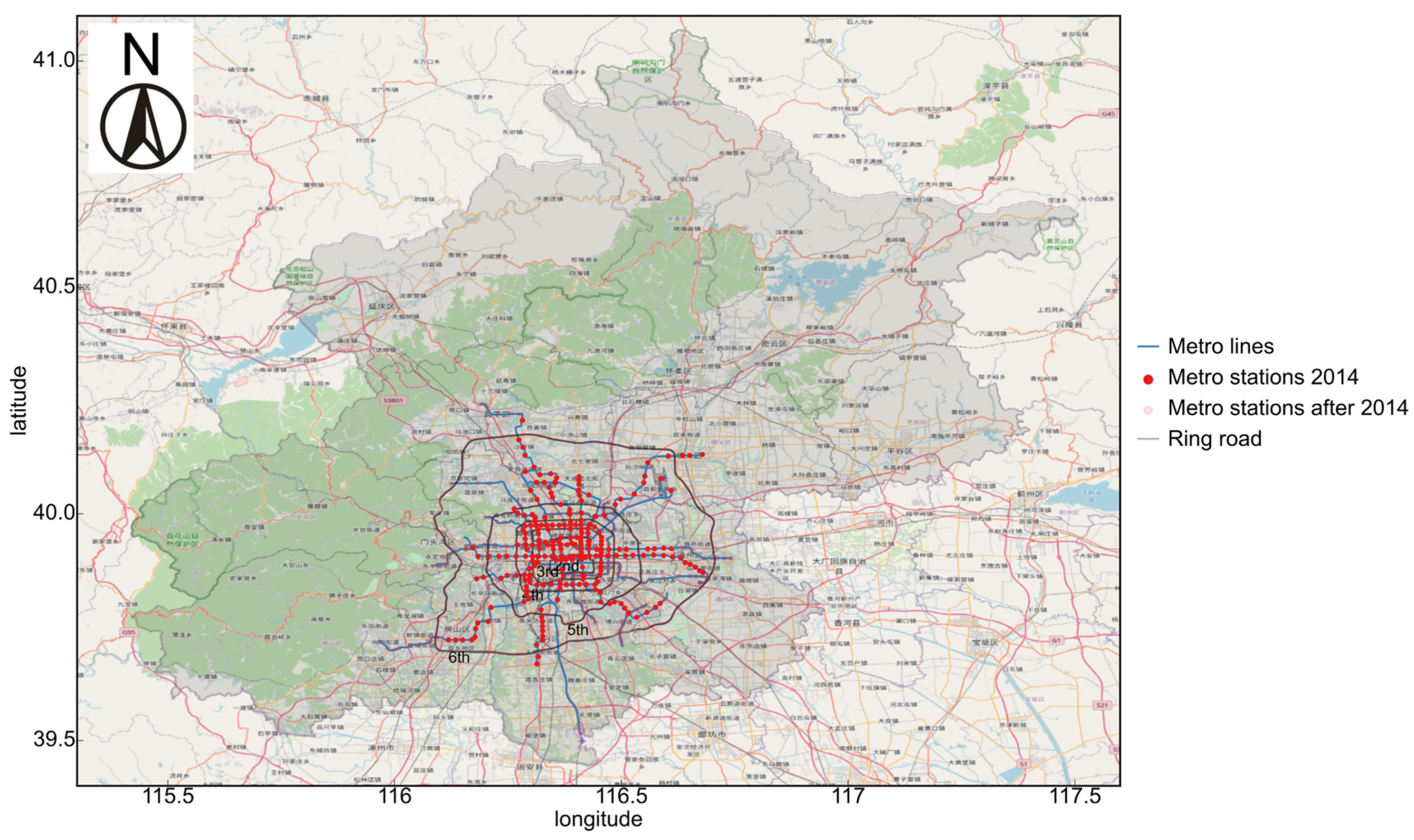
2.1. The Study Area and AFC Data

Beijing is the capital of China with a stable resident population of more than 21 million from 2014 till now. Figure 1 shows a map of the administrative borders of all the districts and the metro systems. The densely populated built urban area is within the fifth ring road. From the inner to the outer are the 2–6th ring roads. The boundaries and the road, as well as the urban rail transit networks, are constructed using the fetched location data from OpenStreetMap [33].

We use 127 million records of the metro network by 12.7 million metro card users from 1st to 31st March 2014. The AFC records include five features, the card ID, entrance station, exit station, entrance time, and exit time. The card ID is a unique identifier for each passenger; thus, we can track the visit pattern of each passenger by selecting all the records of the same card ID.

Table 1. Examples of AFC records for one passenger.

Hashed CardID	Entrance Station	Exit Station	Entrance Time	Exit Time
-3445825934149650544	BaGou	Beijing West Railway Station	2014/3/9 11:35:00	2014/3/9 12:10:42
-3445825934149650544	Beijing West Railway Station	BaGou	2014/3/13 21:17:00	2014/3/13 21:54:15
-3445825934149650544	Renmin University	Beijing West Railway Station	2014/3/24 12:11:00	2014/3/24 12:34:42
-3445825934149650544	Beijing West Railway Station	HuoQiYing	2014/3/26 7:03:00	2014/3/26 7:29:13
-3445825934149650544	BaGou	NanLuoGuXiang	2014/3/29 9:35:00	2014/3/29 10:09:34
-3445825934149650544	BeiXinQiao	BaGou	2014/3/29 12:07:00	2014/3/29 12:44:32

gives some examples of the AFC records. Card IDs are hashed to protect the privacy of the passengers. We construct the visit pattern distribution of stations based on all the passengers related to the station with at least one visit.

2.2. Measuring the Similarity of Distributions

General similarity measures include the Manhattan distance, Euclidean distance, Cosine similarity, and Pearson correlation. The aforementioned similarity measures are not designated for measuring the similarity of distributions. They align the features or attributes to compute a pairwise distance and ignore the relative values of different features. We first introduce two indices for measuring the similarity of distributions and show their drawbacks. Then we illustrate the advantage of Wasserstein distance.

2.2.1. KL Divergence and Sorensen Similarity Index

Measuring the distance between two distributions can also be viewed as measuring the similarity of the distributions. There are many indicators to measure the distance of distributions, such as KL (Kullback–Leibler) divergence. For discrete random variables $P$ and $Q$, the formula for calculating KL divergence is $D_{KL}(P\parallel Q)={{\displaystyle \sum }}_{i=1}^{n}p(P_i)log(\frac{p(P_i)}{p(Q_i)})$. For continuous random variables $P$ and $Q$, and the formula for calculating the KL divergence with the probability density functions are known is $D_{KL}(P\parallel Q)={{\displaystyle \int }}_{-\infty }^{+\infty }p(x)log\frac{p(x)}{q(x)}dx$.

As seen from the definition of KL divergence, if the constituent elements of the two groups of discrete distributed distribution are the same with a different arrangement, the values of the KL divergence will be the same. This index ignores the difference between the quantitative variable values. In addition, the KL divergence is asymmetric, that is, $D_{KL}(P\parallel Q)\ne D_{KL}(Q\parallel P)$. The Appendix A further illustrates this disadvantage using toy distributions.

Since the two-dimensional distribution involved is a discrete one, its distribution can be expressed as a matrix, and all indices to measure the similarity of the matrix can be used. For continuous distribution, a binning strategy can be used to discretize it. A common index to measure matrix similarity is the Sorensen Similarity Index. Essentially, the Sorensen similarity index is the mean of overlapped ratio for all the values, so it can be applied to vectors, matrices, or tensors of higher dimensions.

Therefore, KL divergence and Sorensen similarity index cannot reflect value differences in the distribution. Next, we will introduce the Wasserstein distance.

2.2.2. Wasserstein Distance

Wasserstein distance is defined as the minimum cost required to change one distribution $P$ into another $Q$,

$$W_p(P,Q)={(\underset{J\in \mathcal{J}(P,Q)}{inf}{\displaystyle \int }\Vert x-y{\Vert }^{p}dJ(x,y))}^{\frac{1}{p}}$$

(1)

where $\mathcal{J}$ represents a joint distribution with marginal distribution distributions $P$ and $Q$. When the distribution is one-dimensional,

$$W_p(P,Q)={\left({{\displaystyle \int }}_0^1{\left|G^{-1}(z)-H^{-1}(z)\right|}^p\right)}^{\frac{1}{p}}$$

(2)

where $p$ is the coefficient for an appropriate norm, $G$ and $H$ are the cumulative distribution function (CDF) for $P$ and $Q$, respectively.

The Wasserstein distance of two discrete distributions can be modeled as a transportation problem, which minimizes the total distance cost to change a distribution into another. For two discrete variables $P$ and $Q$, given their distributions and the distance matrix between values of the random variables, determine a matrix $\mathit{F}$ to change from each point of the first distribution to the second distribution, to make the total transportation cost the smallest. Therefore, the two distributions are equivalent to the supply volume and demand volume in the transportation problem, and the distance matrix can be defined to consider the correlation between the variable values, and the transportation problem can be modeled as a linear programming problem:

$$W(P,Q)=\min {{\displaystyle \sum }}_{i=1}^n{{\displaystyle \sum }}_{j=1}^n{f}_{ij}{d}_{ij}$$

(3)

$$s.t.\hspace{1em}\{\begin{array}{c}{{\displaystyle \sum }}_{j=1}^n{f}_{ij}=P_i,\forall i\\ {{\displaystyle \sum }}_{i=1}^n{f}_{ij}=Q_j,\forall j\\ f_{ij}\ge 0,\forall i,j\end{array}$$

(4)

$f_{ij}$ is the decision variable denoting the volume that transports from $i$ to $j$, and $d_{ij}$ denotes the cost to transport a unit from $i$ to $j$. The value $d_{ij}$ is one entry in the cost matrix $\mathit{D}$, which is defined by a cost function and discussed in Section 2.2.3 in more detail. The objective function minimizes transportation costs. The first constraints make sure the quantity shipped from the first distribution is equal to the probability value of each point (supply constraints), the second set of constraints means that the total quantity shipped to the second distribution is equal to the probability value of each point (demand constraints), the third constraints indicate that the transportation volume is non-negative.

Wasserstein distance has three advantages over KL divergence and Sorensen similarity index. First, compared with KL divergence, the cost function can be symmetric, and symmetric distance is more reasonable for many cases, such as a feed to clustering. Second, the ability to customize the cost function makes it able to reflect the similarity between quantitative values of the same feature, Third, it can reflect the correlations between different dimensions for high-dimensional data.

The Wasserstein distance can reflect the correlation of the distribution values, while the KL divergence and the Sorensen similarity index cannot distinguish different mean differences in some cases. Similarly, when it is necessary to consider the correlation of high-dimensional distributions, it can be embodied by an appropriate cost matrix.

2.2.3. Definition of the Cost Function

When only considering one-dimensional objects, the cost function is simply defined as the distance between points, i.e., the absolute value of the difference. For a two-dimensional problem, the cost function is defined as the L1, L2 vector norm calculated using OpenCV [34].

2.3. Clustering Based on Proposed Distribution Similarity

2.3.1. Recap of Clustering Methods

Common clustering algorithms include k-means clustering, hierarchical clustering, and density-based clustering. Readers may refer to [35,36,37] for comprehensive reviews. This paper uses the Wasserstein distance to measure the similarity of the distribution. We mainly focus on illustrating the effect of distribution distance measures, so hierarchical clustering is used to reflect the clustering process.

Hierarchical clustering methods cluster all the data points in a hierarchical manner, which can be represented as a dendrogram. Hierarchical clustering can be agglomerative or divisive. Agglomerative clustering is bottom-up starting from one cluster for each point and merging the similar clusters at each iteration. Divisive clustering is top-down starting from only one cluster and splitting one cluster into multiple clusters at each iteration. We use agglomerative clustering in the case study. For each iteration, which clusters to merge depend on the similarity or distance matrix of clusters. There are several ways to define the distance between clusters with multiple objects.

Single linkage: the distance between two clusters is the minimum of the distances of an object in one cluster to an object in the other cluster.

Complete linkage: the distance between two clusters is the maximum of the distances of an object in one cluster to an object in the other cluster.

Average linkage: the distance between two clusters is the average of the distances of an object in one cluster to an object in the other cluster.

The advantage of hierarchical clustering is that it can reflect the clustering process. The disadvantage is that after the closest clusters are merged, they cannot be separated later, even if the points within the cluster are closer to other clusters, they cannot be re-clustered.

2.3.2. Clustering Evaluation Index

Clustering performed with no ground truth labels cannot be evaluated by using cross-validation and various error indices, but the effect of clustering can still be evaluated. Good clustering results need to meet two conditions: the distance between elements of the same cluster is small, the distance between different clusters is large. For hierarchical clustering, the number of clusters needs to be determined. The commonly used method for selecting the number of clusters is the elbow method, and other clustering evaluation indices include the Silhouette coefficient, Calinski–Harabasz index, and Davies–Bouldin index [38,39].

SSE, defined as the sum of squared errors of the same class is often exploited in the elbow method. In this article, we define a similar index within-cluster distance ratio (SDSC/SD): the ratio of the sum of the distances within the cluster to the sum of the total distances. The elbow method is to select a smaller number of clusters that can include the distance in the same cluster. When the number of clusters increases, it is obvious that the total distance in the same cluster will account for a larger proportion. So, the SDSC/SD decreases rapidly at the beginning and then tends to flatten. Therefore, we show the relationship between SDSC/SD and the number of clusters and use the number of clusters when SDSC/SD tends to be flat as the appropriate number of clusters.

The Silhouette index can evaluate the quality of every point. It is defined by two values: the mean distance $a$ from the same cluster and the mean distance $b$ from the closest cluster, then $s=\frac{b-a}{max(a,b)}$. It can be seen from its definition that the Silhouette index range between −1 and 1. A Silhouette index close to 1 means that the distant points are separated reasonably. We use the Silhouette index to select the best linkage metric.

3. Results

3.1. Constructing Passenger’s Visit Count Distribution

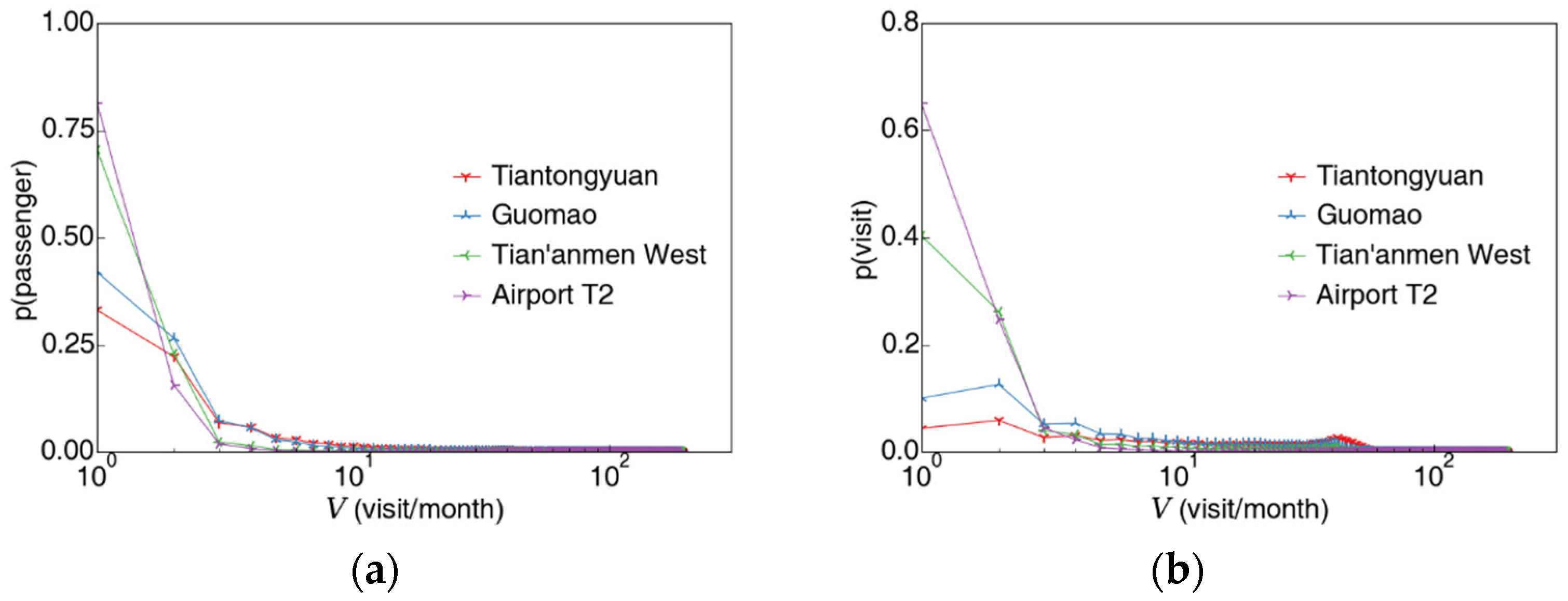
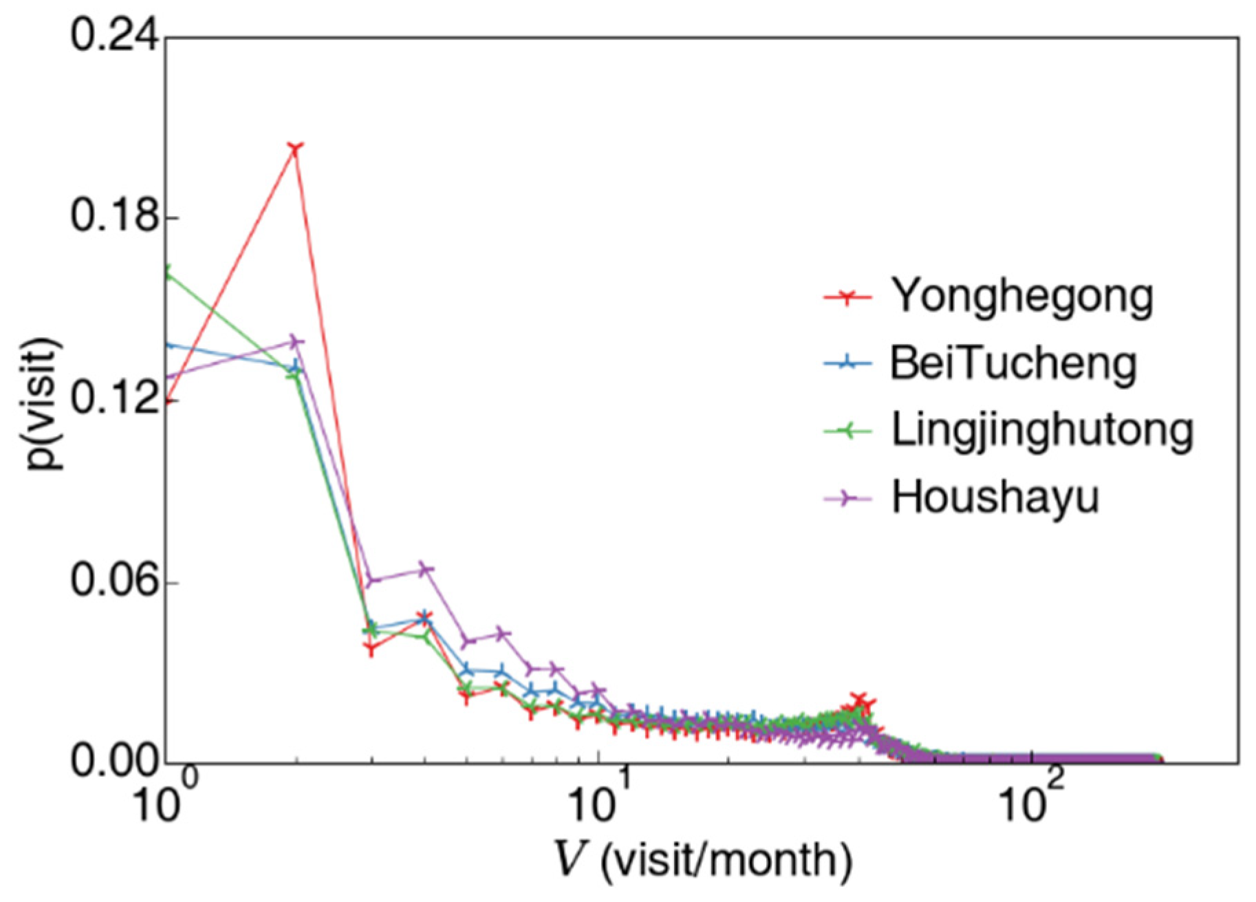
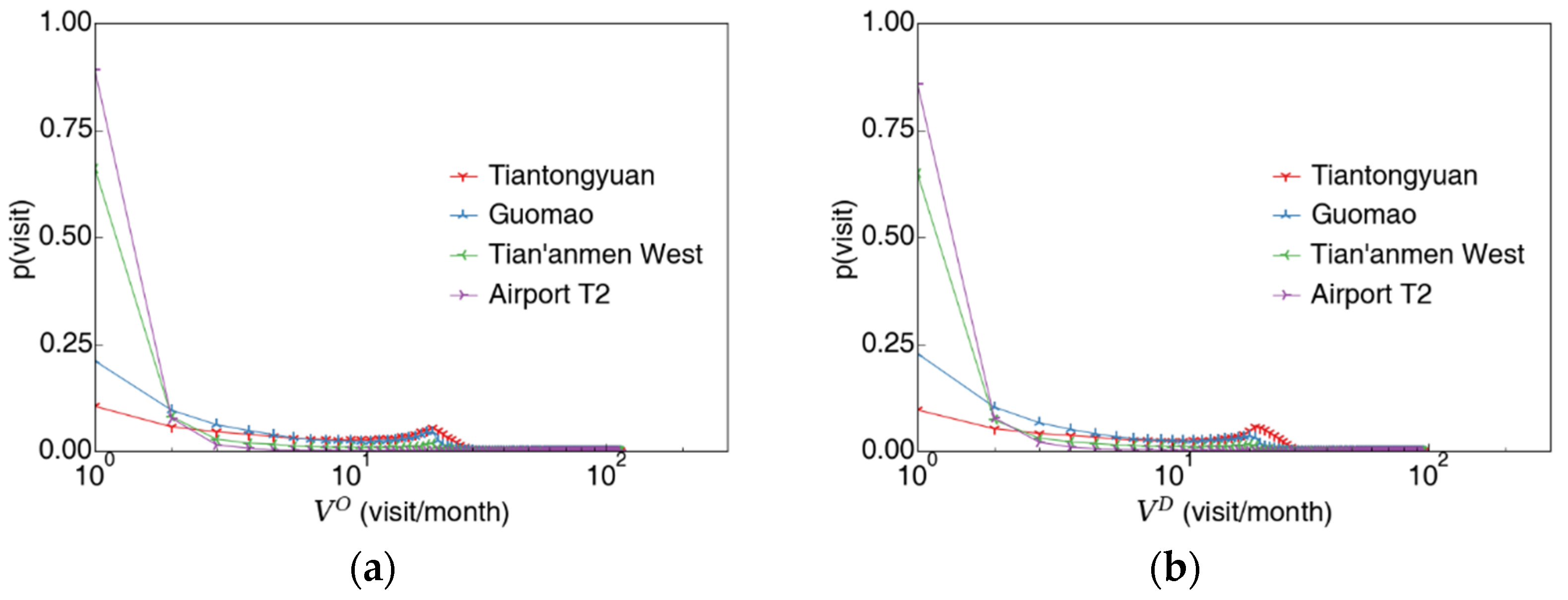
3.1.1. Passenger’s Visit Count to a Certain Station

We first count the visit $v_i^s$ of the passenger $i$ with the station $s$ using the AFC records in one month. It is the sum of trip count with $s$ as the origin and trip count with $s$ as the destination for all trips of passenger $i$. and using the example passenger in Table 1 we obtain the visit count result shown in

Table 2. The visit count to all stations of one passenger.

Hashed CardID	Station	Count
-3445825934149650544	BaGou	4
-3445825934149650544	Beijing West Railway Station	4
-3445825934149650544	Renmin University	1
-3445825934149650544	HuoQiYing	1
-3445825934149650544	NanLuoGuXiang	1
-3445825934149650544	BeiXinQiao	1

. The familiarity of the passenger $i$ with the station $s$ can be described by $v_i^s$. For a specific station $s$, we can build the visit count distribution $V^s$ by using all the passengers with $v_i^s>0$.

We show the proportion of passengers for different visit counts of four typical stations in Beijing Metro in March 2014 in Figure 2a. It can be seen that majority of the passengers visit the Airport T2 station and Tian’anmen West only once or twice, but for Tiantongyuan and Guomao, only about half of the passengers visit once or twice. Figure 2a depicts the overall situation of passengers. In Figure 2b, we investigate the visit pattern as an average snapshot of the station. It is equivalent to using the number of visits as the weight of the passenger distribution.

To check the influence of combined entrance and exit, we also examine the number of visits as the origin and destination respectively, shown in Figure 3. It can be seen that the visit count distribution of passengers entering and leaving the same station is almost the same, reflecting the symmetry of passenger flow distribution.

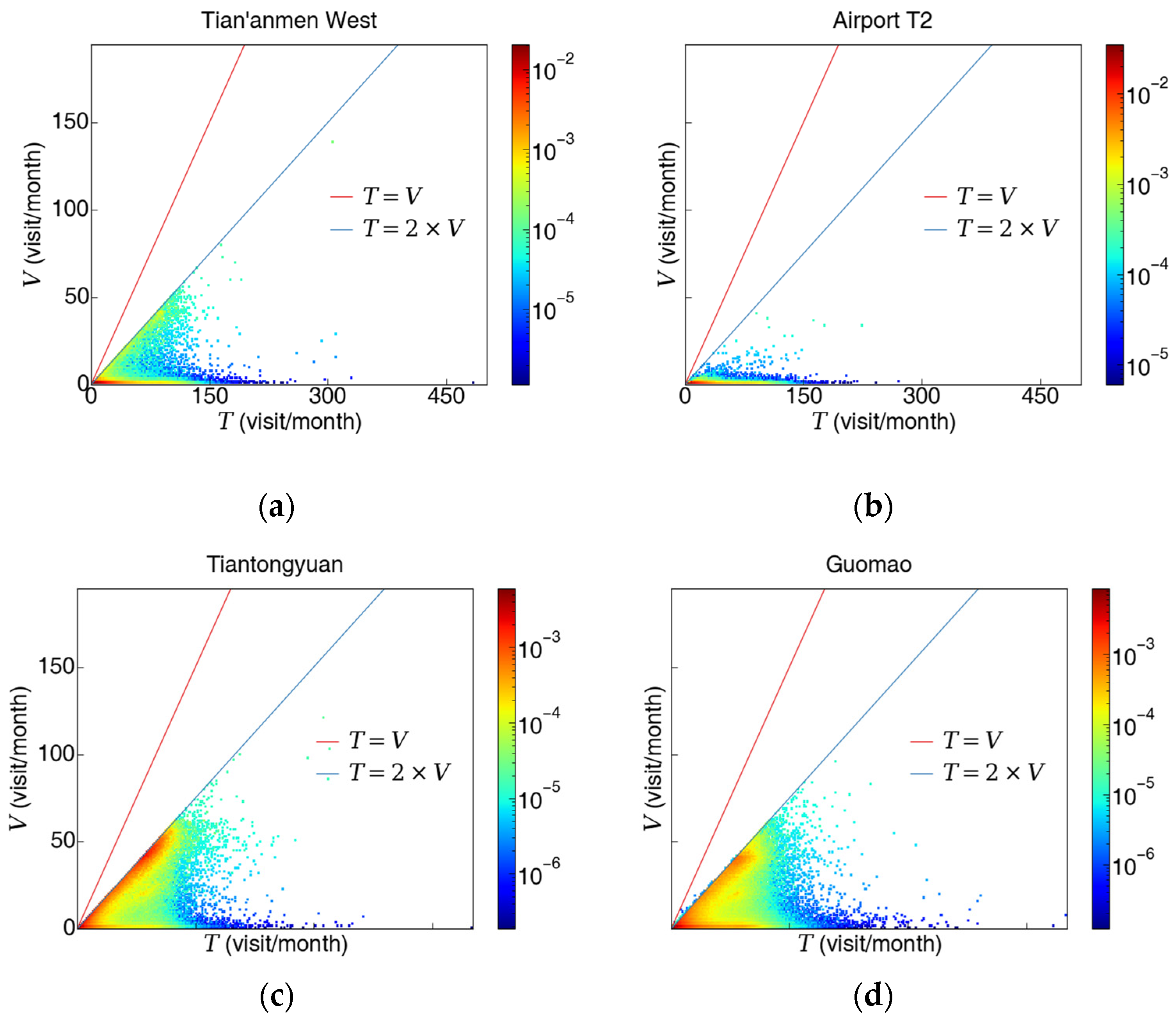
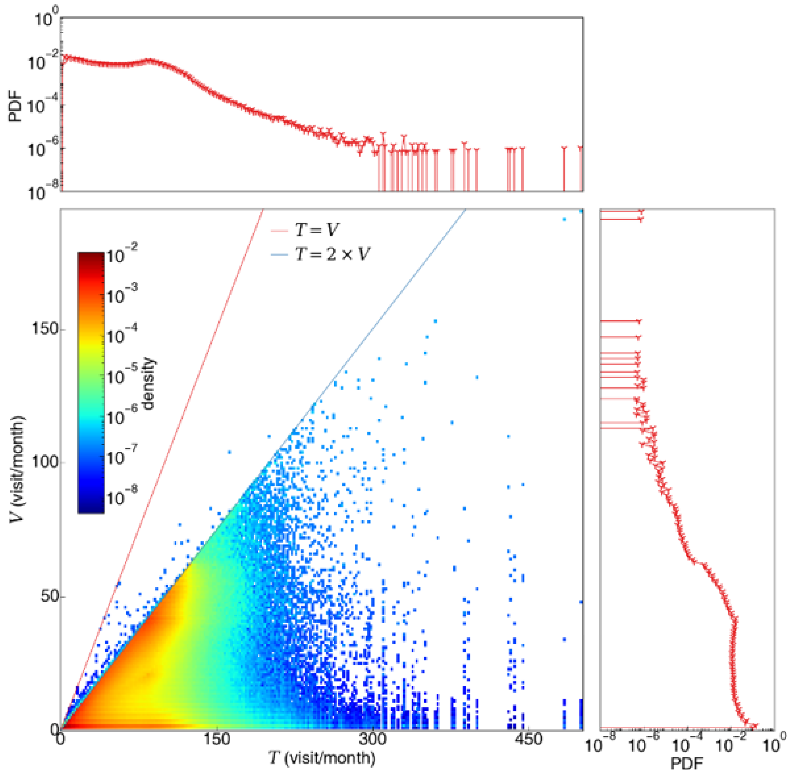
3.1.2. Passenger’s Station-Specific Visit Count and Total Visit Count

In Section 3.1.1, we define the passenger familiarity to a station as the visit count. To reflect the characteristics of the passengers themselves, we add the station-specific visit count and define $t_i={{\displaystyle \sum }}_s{v}_i^s$ as the total visit count to the subway system. We first study the distribution of the visit count of all passengers to the various stations they have visited, and the two-dimensional joint distribution of two random variables: the visit count $V$ and the total visit count $T$, as shown in Figure 4.

The line $T=V$ means that all trips start and end at the same station. This is in that the Beijing Subway allows entry and exit at the same station. In some studies, this kind of data will be cleaned out as abnormal data. $T=2V$ means that a certain station is either the origin or destination for all trips of a certain passenger. It is common for 100% home-based trips when a passenger always starts a journey from home and then returns home afterward. Passengers on this line indicate high familiarity with one station. On the contrary, passengers with $v$ close to one indicate that passengers are not familiar with the station. In short, the two variables $v, t$ jointly characterize the passengers’ familiarity with the station and subway system. There are many passengers along the $T$ axis, who visit certain stations very few times. Moreover, there are some passengers near the line $T=V$, who always visit a certain station. For passengers with a large total visit count, many are distributed in these two areas, and there are few passenger station combinations in-between.

For a station $s$, the random variable $V_s$ represents the distribution of visit count for the station. To more accurately reflect the characteristics of passengers visiting the place, we add $T_s$ to represent the total visit count. Here we show the two-dimensional joint distribution of station-specific visit count and total visit count of four typical stations in Figure 5. We have shown in Section 2.1 that there is a minor difference between entrance and exit, so here we use the combined visit count to define the familiarity. There are mainly two types of passengers for Tiantongyuan, a typical residential station. One is passengers living nearby that almost his every trip starts or ends at Tiantongyuan Station, and the other only visit once or twice, corresponding to passengers visiting relatives and friends. Guomao Station is located in the Central Business District and its passengers are similar to those of Tiantongyuan with fewer passengers near the line $T=V$. The passenger flow of Tian’anmen West is so dominated by tourists that passengers are distributed near the $T$ axis. The Airport T2 is an inter-city transportation hub, so almost all of its passengers are distributed near the $T$ axis, with the most visit of one or two.

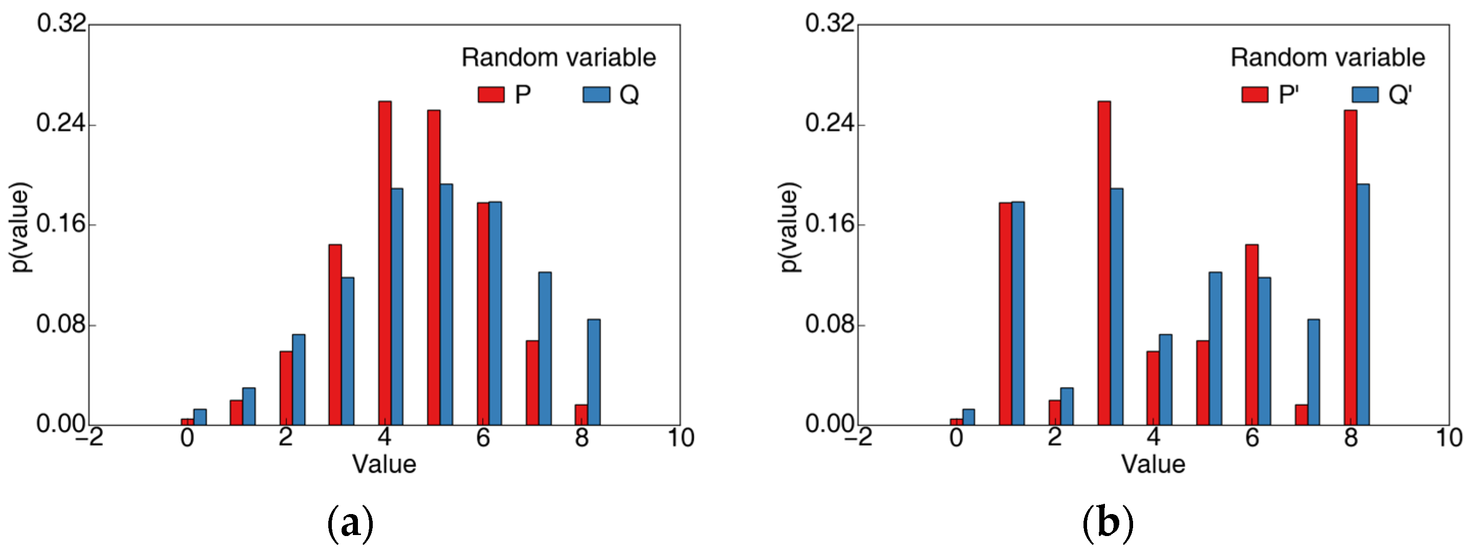
3.2. Illustrating the Advantage of Wasserstein Distance

We further discuss the advantage of Wasserstein distance over the simple mean difference in this section. As shown in Figure 6, the station closest to YongHeGong Lama Temple measured by the mean value is Beitucheng and Lingjing Hutong, and the distribution is closest to Houshayu. Although the average values of Lama Temple, Beitucheng, and Lingjing Hutong are close, the distribution is quite different as shown in Figure 6.

3.3. Clustering Stations Based on Distribution Distance

Using Wasserstein distance, we obtain a distance matrix between all pairs of stations in the Beijing metro system and cluster stations accordingly in this section.

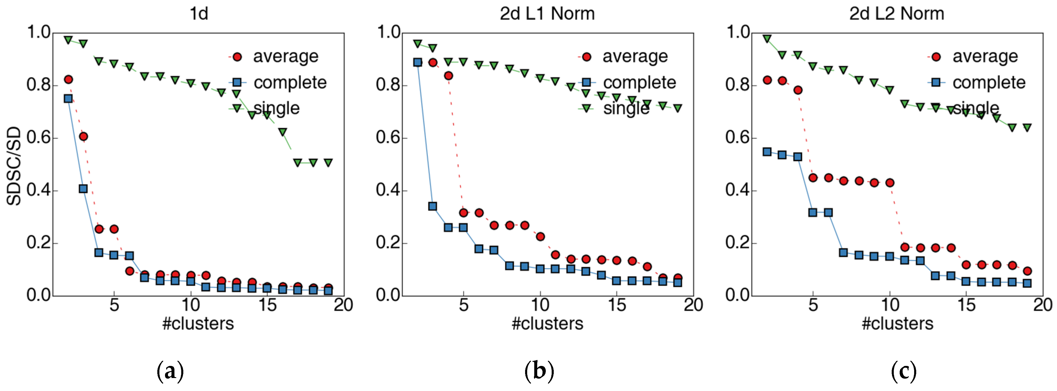
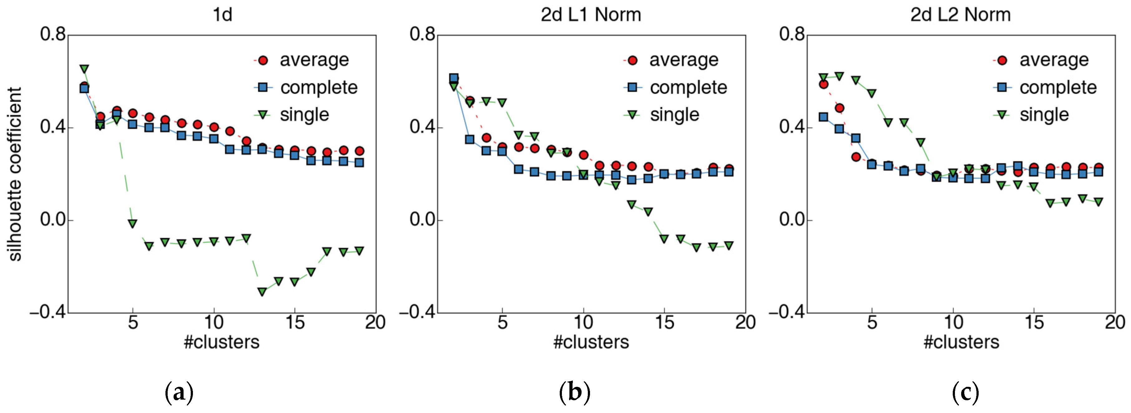
3.3.1. Selection of the Linkage Metric and the Number of Clusters

Clustering and evaluation are implemented using Scikit-learn [21]. We use the number of clusters from 2 to 20, then compare the Silhouette index and the SDSC/SD, shown in Figure 7 and Figure 8. We cluster using one-dimensional Wasserstein distance of station-specific visit distribution and L1 norm and L2 norm for two-dimensional joint distribution considering overall visit count. We use complete linkage considering both the Silhouette index and the SDSC/SD. According to the elbow rule, we select 4/6/7 as the number of clusters correspondingly.

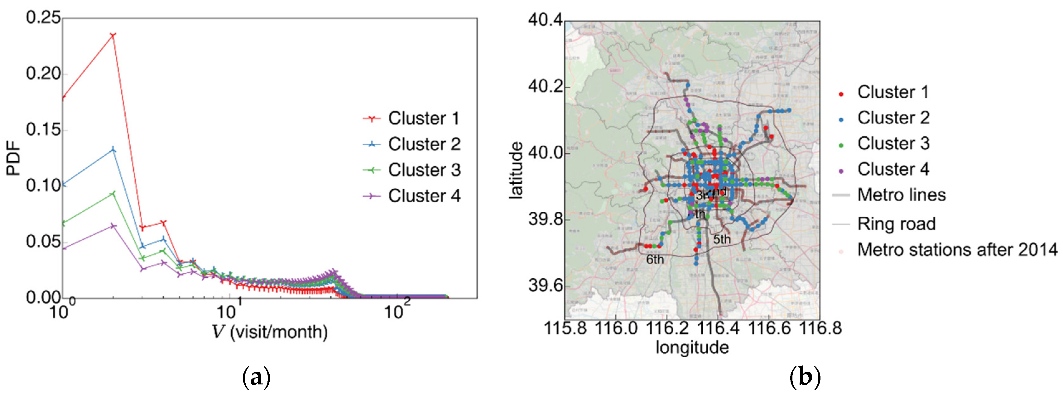
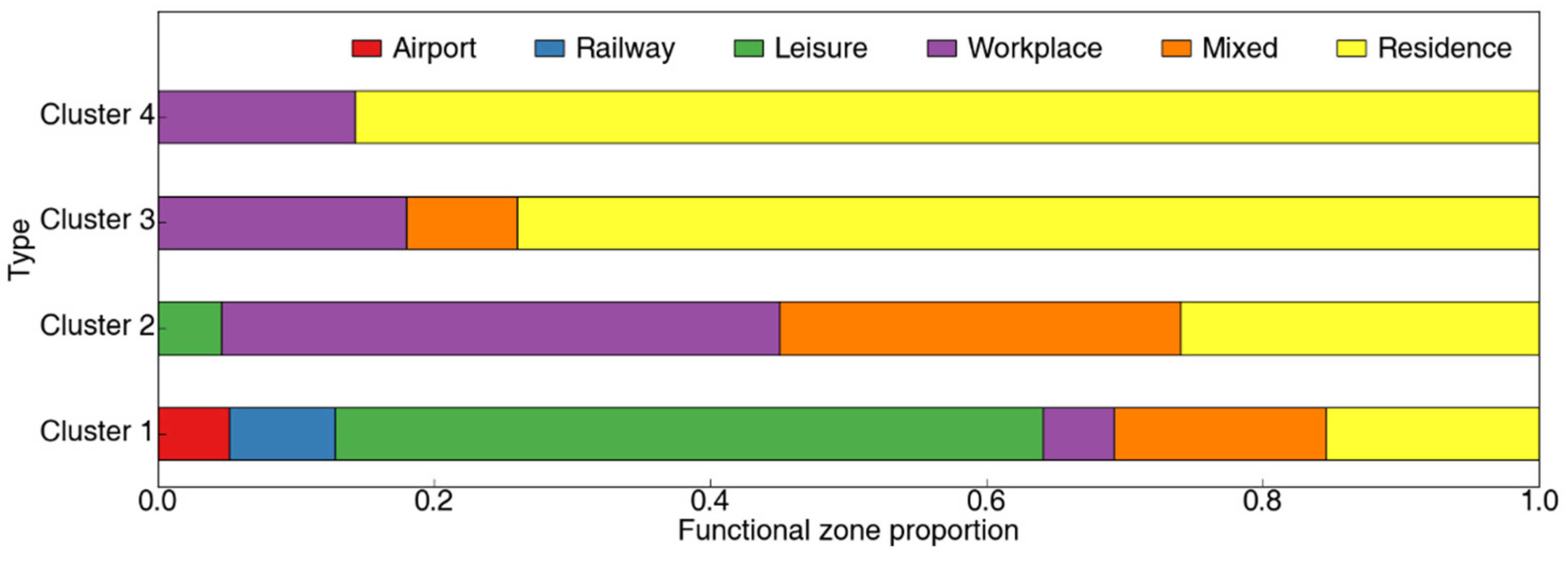
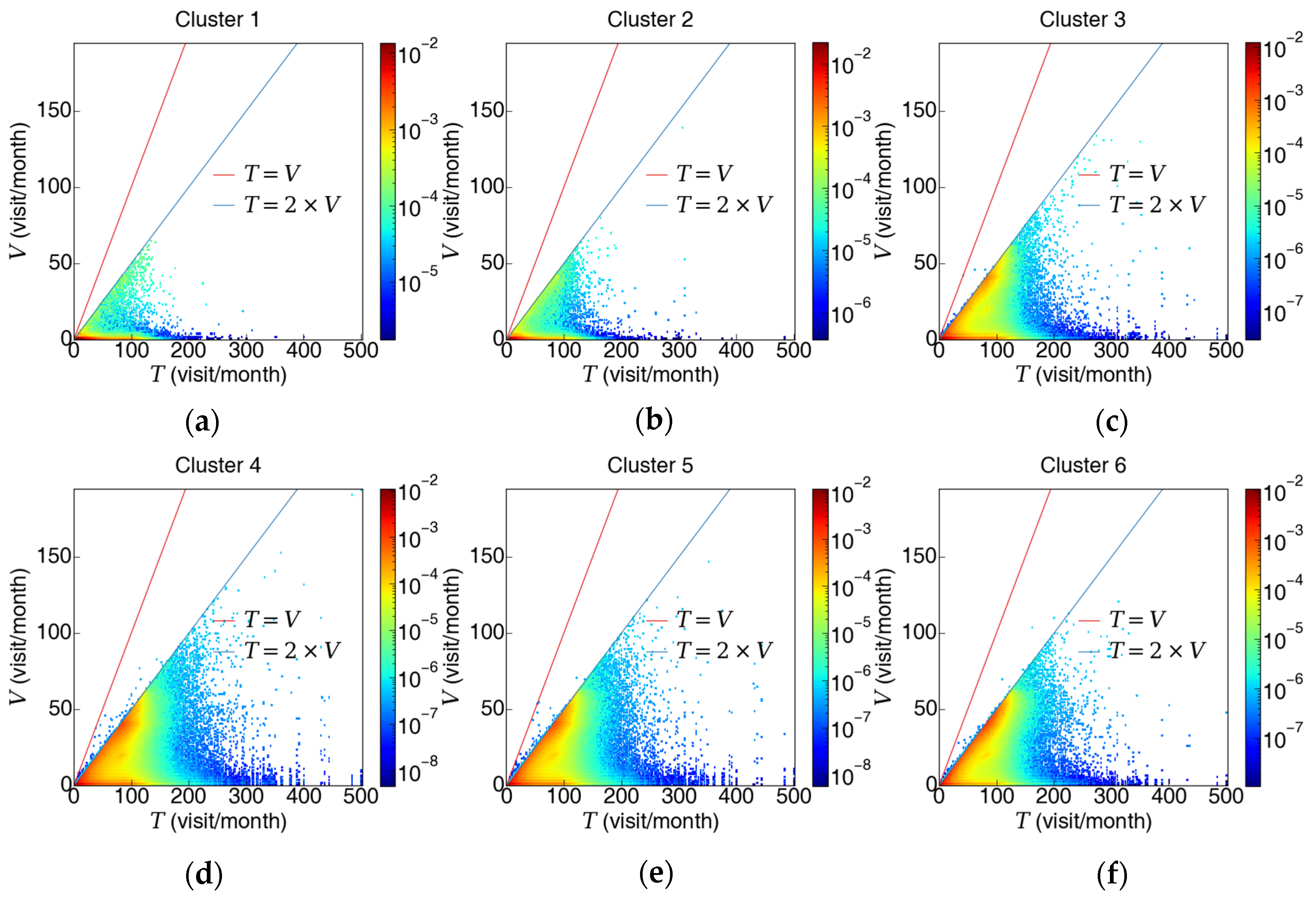
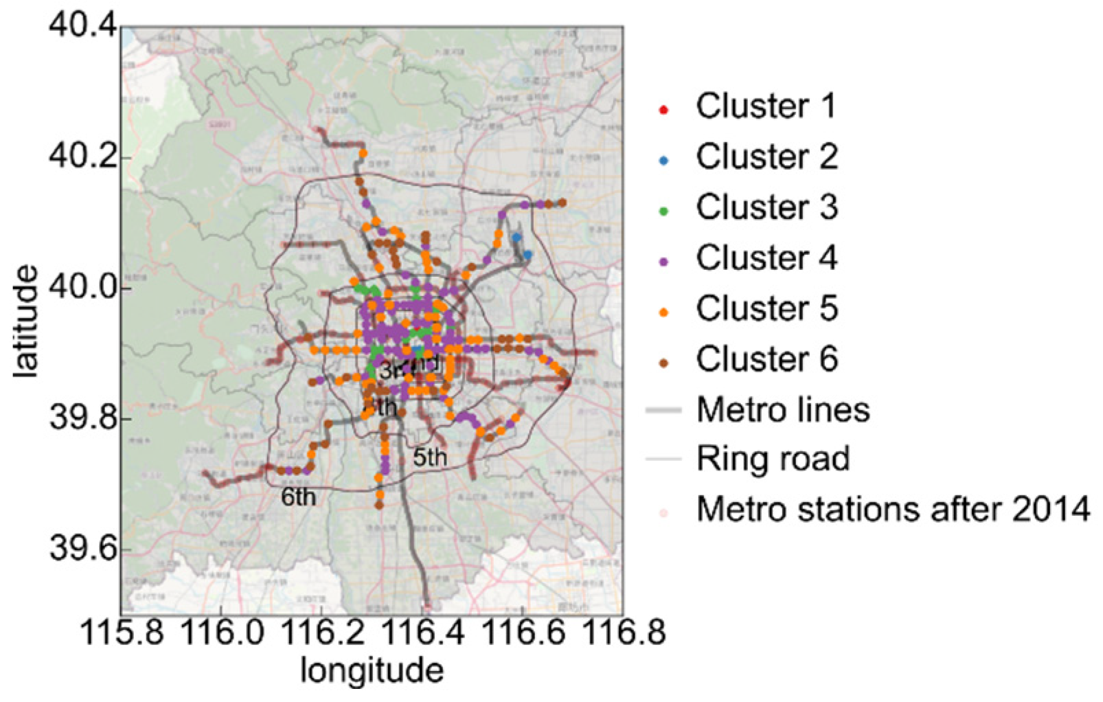
3.3.2. Analysis of Station Visit Distribution Clustering

The results of one-dimensional clustering using only the visit count are shown in Figure 9a,b shows the spatial distribution of stations for each cluster. Stations in Cluster1 have the least familiarity, and the corresponding stations are inter-city transportation hubs and scenic spots, such as airport terminals, railway stations, Tian’anmen, or Beijing Zoo. Cluster 2 contains the largest number of stations, corresponding to working areas and mixed functional areas. Stations in cluster 3 and cluster 4 contain the most familiar passengers, which are related to residential areas.

We further illustrate this by comparing the surrounding functional pattern in each cluster in Figure 10. It can be concluded that the cluster with the most familiar passengers is composed of residential places and the cluster with the least familiar passengers is composed of leisure places

Combining the station-specific visit time and total visit time makes a two-dimensional distribution and the stations clustering results using L1 norm are shown in Figure 11, showing six different passenger clusters. The clustering results using the L2 norm are very similar to this, thus are omitted. The stations corresponding to cluster 1 and cluster 2 corresponds to the lowest proportion of familiar passengers. Cluster 3 is mainly composed of two types of people who are particularly familiar with the site and those who are completely unfamiliar. Cluster 4 and cluster 5 have the widest coverage of passengers, including familiar, unfamiliar, and passengers in-between. The only difference between cluster 4 and cluster 5 is that cluster 4 has more familiar passengers. Cluster 6 is mainly composed of passengers who are particularly familiar with the station. The spatial distribution using the L1 norm is shown in Figure 12.

4. Discussion

We first exploit the AFC data to build the visit count distribution of metro stations to show the passenger familiarity characteristics. Then, using a distribution similarity index, we measure the similarity of stations. This paper also proposes a general method that can cluster distributions. Compared with directly representing the distribution of a feature as a single value, it can reflect the characteristic that the distributions with close values are more similar. The case study of the Beijing Metro network illustrates the effectiveness of the proposed method. We compare the clustering results with the functional zone pattern surrounding the stations, concluding that stations with unfamiliar passengers are related to inter-city transportation hubs and leisure stations while stations with familiar passengers are related to residential places.

There are three drawbacks in this paper. First, the efficient solution to transportation problems is not discussed. For each point, when the scale of the transportation problem is large, the number of variables in linear programming is the square of the number of total intervals of the two-dimensional distribution. Even if polynomial algorithms such as the interior point method are selected, the computational complexity is still high. We simply exploit the OpenCV method without discussing the algorithms. Using heuristic methods to solve the problem does not pursue precise solutions, but can greatly reduce calculation complexity. However, since it is beyond the scope of this article, we only exploit the metric in our clustering method, the heuristic algorithm for transportation problems is not further discussed. Second, no sensitivity analysis is performed on the used cost function. The characteristics of the familiarity of passengers are characterized using simple L1 and L2 norms and we only give a general criterion for choosing the number of clusters for each norm. However, the sensitivity analysis of the cost function is not carried out in the case study. Third, no new clustering algorithm is designed, nor is it theoretically analyzed the pros and cons of each clustering algorithm. On the other hand, this article simply compares the evaluation index values of the hierarchical clustering algorithms.

To reduce the complexity of the problem, some measures that can be adopted include: utilizing truncated distribution, merging adjacent groups in discrete distribution, enlarging the group distance of groups in continuous distribution, and performing matrix decomposition on data and other various dimension reduction methods. Applying a more effective transportation problem algorithm, would speed up the process and make the method more scalable. Moreover, the applicability and performance of different clustering algorithms can be analyzed theoretically.

References

1. Beijing Statistical Yearbook. Available online: http://Nj.Tjj.Beijing.Gov.Cn/Nj/Main/2020-Tjnj/Zk/Indexch.Htm (accessed on 15 November 2021).
2. Wu, J.; Li, D.; Si, S.; Gao, Z. Special Issue: Reliability Management of Complex System. Front. Eng. Manag. 2021, 8, 477–479. [Google Scholar] [CrossRef]
3. Kang, L.; Meng, Q. Two-Phase Decomposition Method for the Last Train Departure Time Choice in Subway Networks. Transp. Res. Part B-Methodol. 2017, 104, 568–582. [Google Scholar] [CrossRef]
4. Liu, L.; Hou, A.; Biderman, A.; Ratti, C.; Chen, J. Understanding Individual and Collective Mobility Patterns From Smart Card Records: A Case Study in Shenzhen. In Proceedings of the 2009 12th International IEEE Conference on Intelligent Transportation Systems, St. Louis, MO, USA, 4–7 October 2009; IEEE: Manhattan, NY, USA, 2009; pp. 1–6. [Google Scholar]
5. Pelletier, M.-P.; Trepanier, M.; Morency, C. Smart Card Data Use In Public Transit: A Literature Review. Transp. Res. Part C-Emerg. Technol. 2011, 19, 557–568. [Google Scholar] [CrossRef]
6. Ma, X.; Wu, Y.-J.; Wang, Y.; Chen, F.; Liu, J. Mining Smart Card Data For Transit Riders’ Travel Patterns. Transp. Res. Part C-Emerg. Technol. 2013, 36, 1–12. [Google Scholar] [CrossRef]
7. Long, Y.; Thill, J. Combining Smart Card Data and Household Travel Survey to Analyze Jobs-Housing Relationships in Beijing. Comput. Environ. Urban Syst. 2015, 53, 19–35. [Google Scholar] [CrossRef] [Green Version]
8. Ma, X.; Liu, C.; Wen, H.; Wang, Y.; Wu, Y.-J. Understanding Commuting Patterns Using Transit Smart Card Data. J. Transp. Geogr. 2017, 58, 135–145. [Google Scholar] [CrossRef]
9. Liu, J.; Shi, W.; Chen, P. Exploring Travel Patterns During The Holiday Season-A Case Study of Shenzhen Metro System During the Chinese Spring Festival. ISPRS Int. J. Geo-Inf. 2020, 9, 651. [Google Scholar] [CrossRef]
10. Hasan, S.; Schneider, C.M.; Ukkusuri, S.V.; González, M.C. Spatiotemporal Patterns Of Urban Human Mobility. J. Stat. Phys. 2013, 151, 304–318. [Google Scholar] [CrossRef] [Green Version]
11. Lei, D.; Chen, X.; Cheng, L.; Zhang, L.; Ukkusuri, S.; Witlox, F. Inferring Temporal Motifs for Travel Pattern Analysis Using Large Scale Smart Card Data. Transp. Res. Part C-Emerg. Technol. 2020, 120, 102810. [Google Scholar] [CrossRef]
12. El Mahrsi, M.K.; Come, E.; Oukhellou, L.; Verleysen, M. Clustering Smart Card Data For Urban Mobility Analysis. IEEE Trans. Intell. Transp. Syst. 2017, 18, 712–728. [Google Scholar] [CrossRef]
13. Deng, Y.; Wang, J.; Gao, C.; Li, X.; Wang, Z.; Li, X. Assessing Temporal-Spatial Characteristics of Urban Travel Behaviors from Multiday Smart-Card Data. Phys. A-Stat. Mech. Its Appl. 2021, 576, 126058. [Google Scholar] [CrossRef]
14. Zhao, J.; Qu, Q.; Zhang, F.; Xu, C.; Liu, S. Spatio-Temporal Analysis Of Passenger Travel Patterns In Massive Smart Card Data. IEEE Trans. Intell. Transp. Syst. 2017, 18, 3135–3146. [Google Scholar] [CrossRef]
15. He, L.; Agard, B.; Trepanier, M. A Classification of Public Transit Users with Smart Card Data Based on Time Series Distance Metrics and A Hierarchical Clustering Method. Transp. A-Transp. Sci. 2020, 16, 56–75. [Google Scholar] [CrossRef]
16. Yang, Y.; Heppenstall, A.; Turner, A.; Comber, A. Who, Where, Why and When? Using Smart Card and Social Media Data to Understand Urban Mobility. ISPRS Int. J. Geo-Inf. 2019, 8, 271. [Google Scholar] [CrossRef] [Green Version]
17. Du, B.; Yang, Y.; Lv, W. Understand Group Travel Behaviors in an Urban Area Using Mobility Pattern Mining. In Proceedings of the IEEE 10th International Conference on Ubiquitous Intelligence and Computing, UIC 2013 and IEEE 10th International Conference on Autonomic and Trusted Computing, ATC 2013, Vietri sul Mare, Italy, 18–21 December 2013; IEEE: Manhattan, NY, USA, 2013; pp. 127–133. [Google Scholar] [CrossRef]
18. Sun, L.; Axhausen, K.W. Understanding Urban Mobility Patterns With A Probabilistic Tensor Factorization Framework. Transp. Res. Part B Methodol. 2016, 91, 511–524. [Google Scholar] [CrossRef]
19. Beijing Municipal Bureau Statistics Beijing Statistical Yearbook. Available online: http://Nj.Tjj.Beijing.Gov.Cn/Nj/Main/2021-Tjnj/Zk/Indexch.Htm (accessed on 22 December 2021).
20. Dong, H.; Wu, M.; Ding, X.; Chu, L.; Jia, L.; Qin, Y.; Zhou, X. Traffic Zone Division Based on Big Data from Mobile Phone Base Stations. Transp. Res. Part C Emerg. Technol. 2015, 58, 278–291. [Google Scholar] [CrossRef]
21. Shen, P.; Ouyang, L.; Wang, C.; Shi, Y.; Su, Y. Cluster and Characteristic Analysis of Shanghai Metro Stations Based on Metro Card and Land-Use Data. Geo-Spat. Inf. Sci. 2020, 23, 352–361. [Google Scholar] [CrossRef]
22. Xiong, L.; Chen, X.; Huang, T.K.; Schneider, J.; Carbonell, J.G. Temporal Collaborative Filtering with Bayesian Probabilistic Tensor Factorization. In Proceedings of the 10th Siam International Conference on Data Mining, SDM 2010, Columbus, OH, USA, 29 April–1 May 2010; SIAM: Philadelphia, PA, USA, 2010; pp. 211–222. [Google Scholar] [CrossRef] [Green Version]
23. Dong, X.; Thanou, D.; Frossard, P.; Vandergheynst, P. Learning Laplacian Matrix in Smooth Graph Signal Representations. IEEE Trans. Signal Process. 2016, 64, 6160–6173. [Google Scholar] [CrossRef] [Green Version]
24. Yu, H.-F.; Rao, N.; Dhillon, I.S. Temporal Regularized Matrix Factorization for High-Dimensional Time Series Prediction. In Proceedings of the Advances in Neural Information Processing Systems 29 (NIPS 2016), Barcelona, Spain, 5–10 December 2016; Lee, D.D., Sugiyama, M., Luxburg, U.V., Guyon, I., Garnett, R., Eds.; Curran Associates: New York, NY, USA, 2016; Volume 29. [Google Scholar]
25. Xu, J. Map Sensitivity vs. Map Dependency: A Case Study of Subway Maps’ Impact on Passenger Route Choices in Washington DC. Behav. Sci. 2017, 7, 72. [Google Scholar] [CrossRef] [Green Version]
26. Lei, B.; Xu, J.; Li, M.; Li, H.; Li, J.; Cao, Z.; Hao, Y.; Zhang, Y. Enhancing Role of Guiding Signs Setting in Metro Stations with Incorporation of Microscopic Behavior of Pedestrians. Sustainability 2019, 11, 6109. [Google Scholar] [CrossRef] [Green Version]
27. Shiwakoti, N.; Tay, R.; Stasinopoulos, P.; Woolley, P.J. Passengers’ Awareness and Perceptions of Way Finding Tools in a Train Station. Saf. Sci. 2016, 87, 179–185. [Google Scholar] [CrossRef]
28. Hong, L.; Gao, J.; Zhu, W. Simulating Emergency Evacuation at Metro Stations: An Approach Based on Thorough Psychological Analysis. Transp. Lett.-Int. J. Transp. Res. 2016, 8, 113–120. [Google Scholar] [CrossRef]
29. Faroqi, H.; Mesbah, M.; Kim, J. Behavioural Advertising In The Public Transit Network. Res. Transp. Bus. Manag. 2019, 32, 100421. [Google Scholar] [CrossRef]
30. Raveau, S.; Guo, Z.; Munoz, J.C.; Wilson, N.H.M. A Behavioural Comparison of Route Choice on Metro Networks: Time, Transfers, Crowding, Topology and Socio-Demographics. Transp. Res. Part A-Policy Pract. 2014, 66, 185–195. [Google Scholar] [CrossRef]
31. Zhu, Y.; Hu, C.; Xu, D.; Tang, J. Research on Optimization for Passenger Streamline of Hubs. Procedia-Soc. Behav. Sci. 2014, 138, 776–782. [Google Scholar] [CrossRef] [Green Version]
32. Lotan, T. Effects of Familiarity on Route Choice Behavior in the Presence of Information. Transp. Res. Part C-Emerg. Technol. 1997, 5, 225–243. [Google Scholar] [CrossRef]
33. Openstreetmap. Available online: https://www.openstreetmap.org/ (accessed on 22 December 2021).
34. Bradski, G. The Opencv Library. Dobb’s J. Softw. Tools 2000, 25, 120–123. [Google Scholar]
35. Fahad, A.; Alshatri, N.; Tari, Z.; Alamri, A.; Khalil, I.; Zomaya, A.Y.; Foufou, S.; Bouras, A. A Survey of Clustering Algorithms for Big Data: Taxonomy and Empirical Analysis. IEEE Trans. Emerg. Top. Comput. 2014, 2, 267–279. [Google Scholar] [CrossRef]
36. Murtagh, F.; Contreras, P. Algorithms For Hierarchical Clustering: An Overview, II. Wiley Interdiscip. Rev.-Data Min. Knowl. Discov. 2017, 7, E1219. [Google Scholar] [CrossRef] [Green Version]
37. Saxena, A.; Prasad, M.; Gupta, A.; Bharill, N.; Patel, O.P.; Tiwari, A.; Er, M.J.; Ding, W.; Lin, C.-T. A Review of Clustering Techniques and Developments. Neurocomputing 2017, 267, 664–681. [Google Scholar] [CrossRef] [Green Version]
38. Pedregosa, F.; Varoquaux, G.; Gramfort, A.; Michel, V.; Thirion, B.; Grisel, O.; Blondel, M.; Prettenhofer, P.; Weiss, R.; Dubourg, V.; et al. Scikit-Learn: Machine Learning in Python. J. Mach. Learn. Res. 2011, 12, 2825–2830. [Google Scholar]
39. Rousseeuw, P.J. Silhouettes: A Graphical Aid to The Interpretation and Validation of Cluster Analysis. J. Comput. Appl. Math. 1984, 20, 53–65. [Google Scholar] [CrossRef] [Green Version]
Figure 1. Metro network in Beijing. The grey polygons show the administrative borders of all the districts. The area inside the 5th ring road is the core urban area and most metro stations are within the 6th ring.
Ijgi 11 00018 g001
Figure 2. The distribution of the number of visits by passengers at four typical stations: (a) The proportion of passengers visiting Tiantongyuan, Guomao (China World Trade Center), Tian’anmen West, and Airport Terminal 2 at a given visit count. The V-axis is shown in the log scale. (b) The distribution of passenger visits, weighted by the number of visits, shows an average snapshot of passenger visit count distribution.
Ijgi 11 00018 g002
Figure 3. The distribution of the number of entrance and exit visits by passengers at four typical stations: (a) The distribution of passenger entrance visits. (b) The distribution of passenger exit visits.
Ijgi 11 00018 g003
Figure 4. The joint distribution of total visit count and station-specific visit count. The panel on the top and the right show the marginal probability distribution of total visit count and station-specific visit count, respectively.
Ijgi 11 00018 g004
Figure 5. The joint distribution of total visit count T s and station-specific visit count V s for four typical stations: (a) Tiantongyuan; (b) Guomao; (c) Tian’anmen West; (d) Airport Terminal 2.
Ijgi 11 00018 g005
Figure 6. The distribution of the number of visits by passengers at four stations: Yonghegong, Beitucheng, Lingjinghutong, and Houshayu related to Yonghegong.
Ijgi 11 00018 g006
Figure 7. The Silhouette index for different numbers of clusters using different linkage metrics: The Silhouette index results using the (a) one-dimensional distribution of the visit count, (b) two-dimensional joint distribution of station-specific and total visit count using L1 norm, (c) L2 norm.
Ijgi 11 00018 g007
Figure 8. The within-cluster distance ratio (SDSC/SD) for different numbers of clusters using different linkage metrics: (a) one-dimensional distribution of the visit count, (b) two-dimensional joint distribution of station-specific and total visit count using L1 norm, (c) L2 norm.
Ijgi 11 00018 g008
Figure 9. Distribution of each cluster: (a) Clustering results using the one-dimensional distribution of the visit count, from cluster 1 to 4, the familiarity increases. (b) Spatial distribution of clusters.
Ijgi 11 00018 g009
Figure 10. The functional zone proportion for different visit distribution clusters.
Ijgi 11 00018 g010
Figure 11. The familiarity distribution of each cluster. From (af), the familiarity increases.
Ijgi 11 00018 g011
Figure 12. Spatial distribution of each cluster in the metro network.
Ijgi 11 00018 g012