Real-Time Dolphin Whistle Detection on Raspberry Pi Zero 2 W with a TFLite Convolutional Neural Network

Abstract

The escalating conflict between cetaceans and fisheries underscores the need for efficient mitigation strategies that balance conservation priorities with economic viability. This study presents a TinyML-driven approach deploying an optimized Convolutional Neural Network (CNN) on a Raspberry Pi Zero 2 W for real-time detection of bottlenose dolphin whistles, leveraging spectrogram analysis to address acoustic monitoring challenges. Specifically, a CNN model previously developed for classifying dolphins’ vocalizations and originally implemented with TensorFlow was converted to TensorFlow Lite (TFLite) with architectural optimizations, reducing the model size by 76%. Both TensorFlow and TFLite models were trained on 22 h of underwater recordings taken in controlled environments and processed into 0.8 s spectrogram segments (300 × 150 pixels). Despite reducing model size, TFLite models maintained the same accuracy as the original TensorFlow model (87.8% vs. 87.0%). Throughput and latency were evaluated by varying the thread allocation (1–8 threads), revealing the best performance at 4 threads (quad-core alignment), achieving an inference latency of 120 ms and sustained throughput of 8 spectrograms/second. The system demonstrated robustness in 120 h of continuous stress tests without failure, underscoring its reliability in marine environments. This work achieved a critical balance between computational efficiency and detection fidelity (F1-score: 86.9%) by leveraging quantized, multithreaded inference. These advancements enable low-cost devices for real-time cetacean presence detection, offering transformative potential for bycatch reduction and adaptive deterrence systems. This study bridges artificial intelligence innovation with ecological stewardship, providing a scalable framework for deploying machine learning in resource-constrained settings while addressing urgent conservation challenges.

1. Introduction

The interaction between cetaceans and fishing activities has been increasingly investigated due to its implications for species conservation, as well as its significant economic impact on fishing activities, resulting from damage to fishing gear and loss of catch [1]. A more recent study shows that this problem has further worsened in recent years [2]. In particular, the phenomenon of depredation, defined as the predatory behavior of marine mammals towards catch or fishing gear, emerged as a significant concern, as discussed in the comprehensive analysis reported by Gonzalo et al. in 2023 [3]. The review presented by Hamer et al. (2012) highlighted that bycatch, defined as the unintended capture of non-target species in fishing gear, is an additional issue to be taken into consideration [4]. A direct approach to mitigating depredation and bycatch involves the use of devices capable of detecting cetacean presence and triggering a response in positive cases [5]. Possible actions include logging interactions for research, notifying cetacean presence via satellite communication, or emitting deterrent sounds. To achieve this, the device should meet three main criteria: accurate detection, affordability, and sustainable power consumption. Various deterrence strategies based on noise disturbances have been tested over time, including acoustic pingers that emit sounds at regular intervals [6] and improved pingers with an interactive approach that detect presence through basic acoustic analysis [7]. However, the results of these approaches have not always been consistent or reliable, as highlighted in previous works by this and other research groups [8,9,10].

A potentially effective solution to this issue lies in the development of intelligent robotic systems capable of real-time detection and interpretation of dolphin vocalizations, thereby enabling timely interventions to deter dolphins from approaching. The work of the authors of the present study is situated within this research framework. Indeed, the overall aim of the work-in-progress project is to develop an interactive acoustic device to detect the presence of dolphins using Convolutional Neural Network (CNN) models and generate disruptive sounds to dissuade the dolphins from approaching. The hardware of this device is characterized by a Single Board Computer (SBC) supported by a Power Management Module (PSU) utilizing a LiPo battery and an audio input/output device, consisting of the home-made, low-cost CoPiDi hydrophone, introduced and characterized in a previous study [11], coupled with a preamplifier based on low-noise, low-power operational amplifiers. From a software perspective, a modular approach is adopted. A preliminary stage performs real-time digital signal processing (DSP) to identify signal variations warranting further investigation. When triggered, the system processes the signal to generate spectrogram images, which are then fed into a binary CNN trained to classify bottlenose dolphin whistles. Upon a positive detection, the system logs the event timestamp and the corresponding signal segment (for post-deployment analysis) and activates a deterrent sound. This dual functionality ensures both immediate intervention and continuous improvement of detection accuracy through data-driven model updates. Among the key characteristics that deterrent devices must possess, sustainable cost represents the most critical aspect. Fishery operators, particularly in small-scale fisheries, lack substantial financial resources to invest in complex acoustic systems. Furthermore, certain fishing practices (e.g., gillnets) may require the deployment of numerous deterrent units to cover extensive areas.

The role of this specific investigation within the broader project is to identify a solution that allows for the integration of the computational software (CNN) into the designated robotic device, ensuring full compliance with its technical specifications. A modern and promising approach involves tiny machine learning (TinyML)-enabled devices. TinyML represents an emerging field in machine learning that focuses on developing algorithms and models capable of running on low-power devices with limited memory [12]. Unlike traditional Machine Learning (ML) models, which require significant computing resources, TinyML enables real-time recognition on small, low-power devices. The TinyML ecosystem includes a range of devices, from 32-bit microcontroller units (MCUs) to multicore 64-bit ARM CPUs [13], along with supporting libraries.

In a previous study, we attempted to address the issue of detecting the dolphin presence by using a convolutional neural network trained on spectrograms of dolphin whistles [14]. In addition to this study, in recent years, several researchers have investigated the use of artificial intelligence (AI) models for the detection of dolphin presence, with a particular focus on whistle analysis through spectrogram processing [15,16,17]. Indeed, cetaceans communicate through whistles, which are frequency-modulated acoustic signals that vary between species and context. The bottlenose dolphin emits whistles with frequencies up to 24 kHz and a duration usually ranging from 0.1 to 5 s. Dolphins can also produce a particular and personal signature whistle that permits the precise identification of a single animal. These are the main reasons why some recent studies suggest the employment of a whistle associated with neural networks to improve the performance of dolphin monitoring tasks. Specifically, Nur Korkmaz et al. reported that neural networks can enhance the identification of dolphin whistles from underwater audio recordings, even in the presence of significant environmental noise [15]. Similarly, an increase in whistle identification performance was also reported in a study based on the semantic segmentation of dolphin whistles by neural networks [16]. Deep learning techniques were also successfully employed for the traditional purpose of detecting and then classifying dolphin whistles into different classes [17]. Most of these approaches in the field of dolphin whistle detection and classification rely on Convolutional Neural Networks (CNNs). Collectively, these methods underscore the power of AI for bioacoustic monitoring but also reveal a critical gap: the absence of truly embedded, low-power solutions capable of real-time, on-device inference in marine settings.

Thus, the current aim is to propose a novel TinyML-based approach for real-time detection of bottlenose dolphins via a Raspberry Pi Zero 2 W (hereafter referred to as RPi Zero 2 W) [18] used as an SBC. Specifically, this study focuses on the CNN detector component, involving the conversion and optimization into TensorFlow Lite (TFLite) of a previous CNN model developed and implemented with TensorFlow [14]. This conversion has been performed to ensure that the procedure complies with the key requirements, including high-rate, near-real-time detection, and efficient resource utilization. The primary objective is to assess the computational performance of the RPi Zero 2 W to determine whether it can effectively run the existing CNN model for real-time recognition of dolphin whistles. RPi Zero 2 W was selected as the embedded platform for this study because of its adequate balance of computational power, memory capacity, and energy efficiency, which is critical for real-time cetacean whistle detection in resource-constrained marine environments. Unlike MCUs such as ESP32-S3—which are limited to single/dual-core processors and less than or equal to 512 KB RAM (Random Access Memory) [19]—the chosen board features a quad-core 64-bit ARM (Advanced RISC Machine) Cortex-A53 CPU (Central Processing Unit) clock at 1 GHz and 512 MB LPDDR2 SDRAM. This architecture enables concurrent execution of high-speed audio acquisition (up to 192 kS/s via external devices), Digital Signal Processing (DSP) tasks (e.g., bandpass filtering, FFT computation), and machine learning inference via TensorFlow Lite, all while maintaining deterministic latency under 1 s.

2. Materials and Methods

2.1. Training Dataset and Original CNN Models

This study employed a dataset based on 22 h of continuous acoustic recording of Bottlenose Dolphin (Tursiops truncatus) vocalizations held at the Oltremare thematic marine park in Riccione, Italy, in November 2021. This dataset was employed in a previous work in which we used a TensorFlow model to identify dolphin whistles from audio recordings. A data paper that provides a detailed description of the present dataset is currently being prepared and will soon be submitted to a journal. In the meantime, further details about the dataset can be found in our previous study based on it [14]. A UREC384K acoustic recorder, equipped with an SQ26-05 hydrophone (sensitivity: −193.5 dB re 1 V/μPa@20 °C, in the range of 1 Hz–28 kHz) was used to acquire ambient noise and dolphin vocalizations, sampling the signal in 5 min length wav files at 192 kS/s with a resolution of 16 bits. The acquired signals were min-max normalized to the [0, 1] range and subsequently filtered via a 3–24 kHz band-pass filter. Each 5 min recording block was visually inspected by a trained Passive Acoustic Monitoring (PAM) expert and labeled using Audacity (version 2.4.2). Spectrograms (NFFT = 512, size = 300 × 150 pixels, greyscale) were generated via a Hanning window with 50% overlap with a custom Python (Release 3.11.9) script and segmented into 0.8 s intervals—with each whistle centered—and singularly saved. The 0.8 s duration was chosen because it statistically encompasses nearly all whistles. Signals exceeding 0.8 s were divided into overlapping segments (50% overlap) to ensure complete coverage.

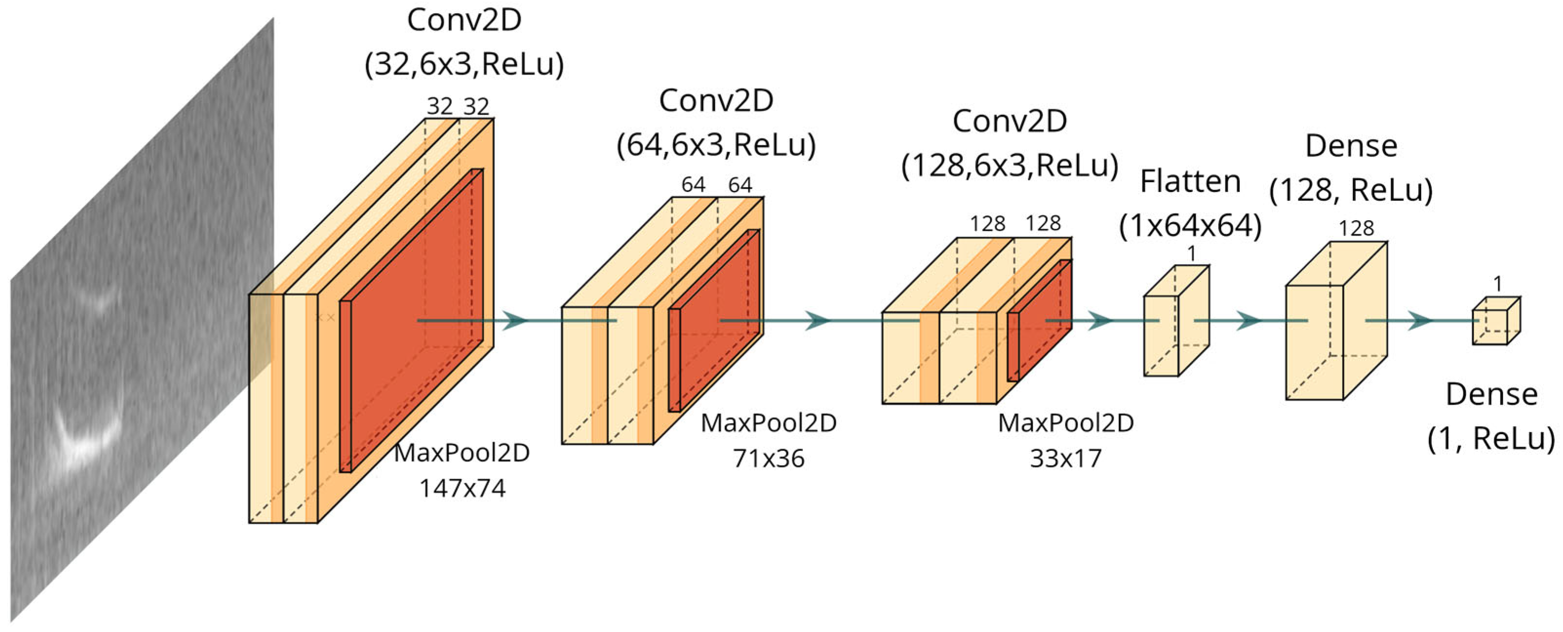
The CNN architecture of the TFLite model, shown in Figure 1, is identical to the original TensorFlow model, and was implemented here for binary classification of the signals, classifying audio segments in positive (whistle-detected) and negative (ambient noise or other sounds). The network comprises three convolutional layers with 32, 64, and 128 filters (convolutional kernel size 6 × 3), each employing Rectified Linear Unit (ReLU) activation, followed by a 2 × 2 max pooling layer to reduce spatial dimensions and mitigate overfitting. The resulting feature maps are flattened and processed by a dense layer with 128 ReLU-activated units, culminating in a single-neuron dense layer with sigmoid activation for classification. A total of 3000 spectrogram images containing dolphin whistles (positive samples) and 3000 spectrogram images featuring ambient noise or no-whistle vocalizations (negative samples) were used to train the CNN using a 10-fold cross-validation approach.

The 3000 positive samples consist of all individual whistle contours detected in the Oltremare dataset, derived from 24 h of continuous recordings in a controlled environment with seven bottlenose dolphins (Tursiops truncatus). The 3000 negative samples were randomly selected from segments of ambient noise and non-whistle vocalizations (e.g., clicks, feeding buzzes), with their quantity matched to the positive samples to ensure class balance during training.

The TFLite models were not trained independently but were generated by converting the original Keras models (exported in the h5 format [20]), which had a size of 107.3 MB each.

2.2. Embedded System Specification

The experimental hardware comprised a Raspberry Pi Zero 2 W Rev 1.0 board: a cost-effective USD 15 single-board computer. This unit is powered by a quad-core 64-bit ARM Cortex-A53 processor running at 1 GHz, supported by 512 MB of LPDDR2 memory, and features integrated Wi-Fi/Bluetooth connectivity and SPI/I2C through the GPIO port. The CPU had a dedicated heatsink (model RP02-HEATSINK, dimensions: 14 × 14 × 4 mm). Data storage was provided by an 8 GB SanDisk Ultra SD card. The software environment was built on a Raspberry Pi OS Lite 64-bit platform. The system operated on kernel version 6.6.51+rpt-rpi-v8 (#1 SMP PREEMPT Debian 1:6.6.51-1+rpt3, 2024-10-08, aarch64). The experimental framework utilized a suite of Python libraries: numpy (v1.26.4) for numerical computations, Pillow (v11.1.0) for image manipulation, scipy (v1.15.1) for scientific computing, scikit-learn (v1.6.1) for machine learning, and TFLite_runtime (v2.14.0) for deploying TensorFlow Lite models.

2.3. Model Conversion and Optimization

The deployment of machine learning models on resource-constrained embedded systems, such as the RPi Zero 2 W, necessitates architectural adaptations to reconcile computational demands with hardware limitations [21]. Non-optimized models were generated by converting pre-trained Keras models into TFLite format without applying any optimization techniques. A Python script was used to automate this process, iterating over ten models saved in the h5 format. Each model was sequentially loaded and converted via the tf.lite.TFLiteConverter.from_keras_model API, which transforms the computational graph into a TFLite-compatible format while maintaining its original structure. This approach preserves the full precision of the original models but does not apply quantization or other optimizations to reduce the memory footprint or improve the inference speed.

The optimized conversion was performed via TensorFlow Lite via the above-mentioned API, which reconfigures the computational graph of the original Keras model into an efficient format suitable for single-board computers. Specifically, after loading the Keras model, the converter was configured with default optimizations (tf.lite.Optimize.DEFAULT) and set to support both standard TFLite built-in operators and TensorFlow operators as a fallback [22]. Moreover, adjustments were made to constrain the use of version 11 for fully connected layers by disabling the experimental lowering of tensor list operations and per-channel quantization, thereby ensuring uniform quantization. Post-training quantization was deliberately omitted because of its propensity to induce significant accuracy degradation, stemming from nonlinear distortions during spectrogram input preprocessing and the absence of quantization-aware training. This conversion strategy effectively balances computational efficiency with model performance on resource-limited hardware. The converter non-optimized models have a size of 37.5 MB for each model file, whereas the optimized version has a size of 9 MB.

2.4. TinyML Paradigm Applied on Resource-Constrained Hardware

Tiny machine learning (TinyML) represents a significant advancement in embedded artificial intelligence, enabling the deployment of machine learning models directly on resource-constrained devices such as microcontrollers or single-board computers. Unlike conventional ML approaches that require server-grade hardware or cloud infrastructure, TinyML leverages highly optimized models (both in terms of memory footprint and computational latency), making it ideal for real-time, low-power, and cost-sensitive applications.

In this work, the TinyML paradigm is realized by converting and optimizing a TensorFlow-based convolutional neural network (CNN) into a TensorFlow Lite (TFLite) format, and subsequently deploying it on a Raspberry Pi Zero 2 W. The key constraints addressed by this implementation are as follows:

• Memory efficiency: Reducing the model size from 37.5 MB to 9 MB enables execution on a device with 512 MB shared RAM.
• Latency constraints: Inference time was reduced from approximately 200 ms to 120 ms, thus supporting near-real-time detection of 0.8 s whistle events.
• Energy and thermal management: Optimized models operate under a significantly lower thermal envelope, reducing the risk of thermal throttling under sustained load.

Importantly, the neural network architecture remains identical to the original TensorFlow model and the non-optimized and optimized TFLite versions. The optimization process does not alter the number of layers, filter sizes, or activations. Instead, it focuses on computational refinements: replacing floating-point operations with quantized counterparts, fusing compatible operations to reduce execution overhead, and using efficient TFLite runtime operators specifically designed for embedded hardware.

2.5. Performance Measurement

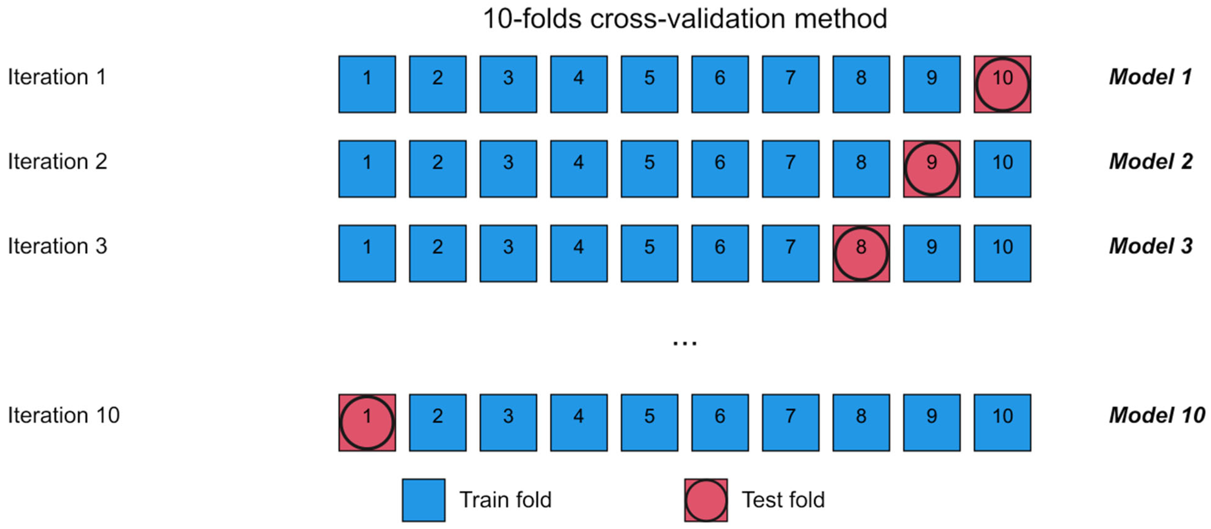
CNN performances were evaluated via the average values of accuracy (“Acc.”), precision (“Prec.”), recall, and F1-score (“F1”), which were computed over ten folds. These metrics are derived from the counts of true negatives (TNs), false negatives (FNs), true positives (TPs), and false positives (FPs). The purpose of 10-fold cross-validation is to assess the generalization performance of the CNN model. By splitting the dataset into 10 equal folds, the model is trained on 9 folds and tested on the remaining one. This process is repeated 10 times, each time using a different fold for testing. The results are then averaged to provide a more robust estimate of model performance on unseen data. This technique helps reduce the risk of overfitting and ensures that the evaluation is not dependent on a single train-test split [23]. The workflow of this procedure is detailed in Figure 2.

Given the limited resources available on the RPi Zero 2 W, additional system monitoring was conducted during the experiments. In particular, the CPU load was tracked by collecting per-core statistics, and the internal processor temperature and memory status (used, free, and total memory) were also recorded. An important parameter considered in this study is the number of spectrogram images processed per second (it/s) obtained by dividing the number of images composing a single batch job by the total time taken by the TFLite mode to process them.

2.6. Latency Benchmarking of the Models

An inference latency analysis was conducted on both the optimized and non-optimized versions to evaluate the performance of the CNN models generated via the ten-fold approach.

Evaluation Procedure:

• Model loading and initialization: The models were loaded using the TFLite-runtime library, and tensor allocation was performed to prepare each model for inference.
• Input generation: For each model, a random input tensor was generated via the NumPy library according to the required input shape, with values in the float32 format within the range of 0–1.
• Latency benchmarking: Before latency measurement, a warm-up phase of five inference executions was performed for each model to mitigate initialization overhead. After this, each model underwent 500 consecutive inference executions. For each execution, the inference time (in milliseconds) was measured using the time.time() function, which is computed as the difference between the recorded start and end timestamps.
• Data collection and analysis: For each model, the average, minimum, and maximum latency values were calculated and recorded, resulting in a complete latency distribution.

2.7. Throughput Estimation Based on Stress Computing Tests

2.7.1. Test Dataset Composition

A dataset comprising 823 positive and 823 negative grayscale spectrogram images—each measuring 300 × 150 pixels and representing 0.8 s of signal—was employed to evaluate the CNN’s performance in computing the latency. These spectrograms were generated from a three-hour recording segment that was entirely excluded from the training process. The methodology and dataset replicate those described for the original TensorFlow model [14], thereby facilitating direct comparisons of the results.

2.7.2. Model Testing Procedure

A custom Python script was developed to evaluate each model generated via 10-fold cross-validation. The evaluation process proceeds as follows:

• The selected model is loaded into memory.
• The positive and negative images are divided into four blocks of approximately equal size, with each block containing a balanced mix of 50% positive and 50% negative samples.
• For each block:
• All the images are loaded into memory, and the corresponding ground-truth matrix is generated.
• The images are then processed sequentially by the model, with the resulting predictions appended to a list.
• The performance statistics are computed by comparing the predictions to the ground truth.
• Global metrics for the model are generated.

An important feature of the Python script is the ability to define the number of thread instances utilized for model execution explicitly. This is achieved by specifying the desired number of threads (parameter: num_threads) within the TFLite.Interpreter function. This parameter was tested with values ranging from 1–8. The optimized and non-optimized models were tested separately.

2.7.3. System Resource Monitoring

In parallel, a C program (compiled with a -02 flag) was executed to monitor system performance. It samples system metrics every 0.1 s, collects memory status from /proc/meminfo, per-core load from /proc/stat, and CPU temperature from /sys/class/thermal/thermal_zone0/temp.

$$U_{\left[t\right]\left[i\right]}={\displaystyle \frac{{Cbusy}_{\left[t\right]\left[i\right]}-{Cbusy}_{\left[t-1\right]\left[i\right]}}{{Ctotal}_{\left[t\right]\left[i\right]}-{Ctotal}_{\left[t-1\right]\left[i\right]}}}$$

(1)

The CPU usage is determined via Formula (1), where t refers to the time series and i to the CPU core instance (1–4).

The Python script communicates with the monitoring process via an inter-process pipe, transmitting the current test execution state (image loading into memory, TFLite model inference, or statistical computation). This allows the system to differentiate and annotate the measured system information in the log files based on the specific task being performed.

Each test was repeated ten times to ensure a robust statistical dataset. Given the ten different models, each executed with thread counts varying from 1 to 8, and considering both optimized and non-optimized versions, a total of 800 executions were performed for both the non-optimized and the optimized versions. The experiments were carried out at an ambient temperature of 18 °C.

Memory usage during tests was estimated via an ad hoc Python script through the function memory_info().rss of the psutils.Process() library. This program measures the resident set size (RSS) memory consumption across five critical phases:

• Post library initialization;
• Synthetic image dataset generation of a given number (fixed shape 1 × 300 × 150 × 1);
• Model loading via a buffer file with a specified num_threads value;
• Tensor allocation initiated by a single image processing bootstrap;
• Batched inference execution.

The tool parameterizes the model optimization type (optimized vs. non-optimized), thread count (1–8), and input volume (1, 5, 50, and 250 images). The results were stored in CSV format, capturing differential memory utilization between phases.

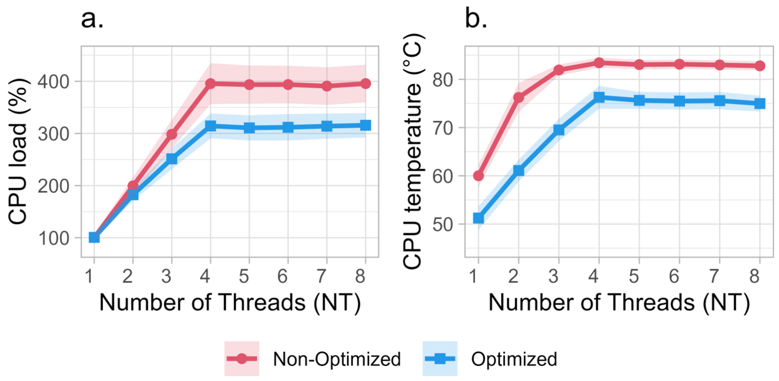
Since the Raspberry Pi Zero 2 W features a quad-core processor, total CPU usage can exceed 100%. For instance, a load of 200% indicates that two cores are fully utilized, while a load of 400% corresponds to full utilization across all four cores. Throughout this manuscript, CPU usage values refer to the cumulative load across all cores.

2.7.4. Parallel Inference Analysis

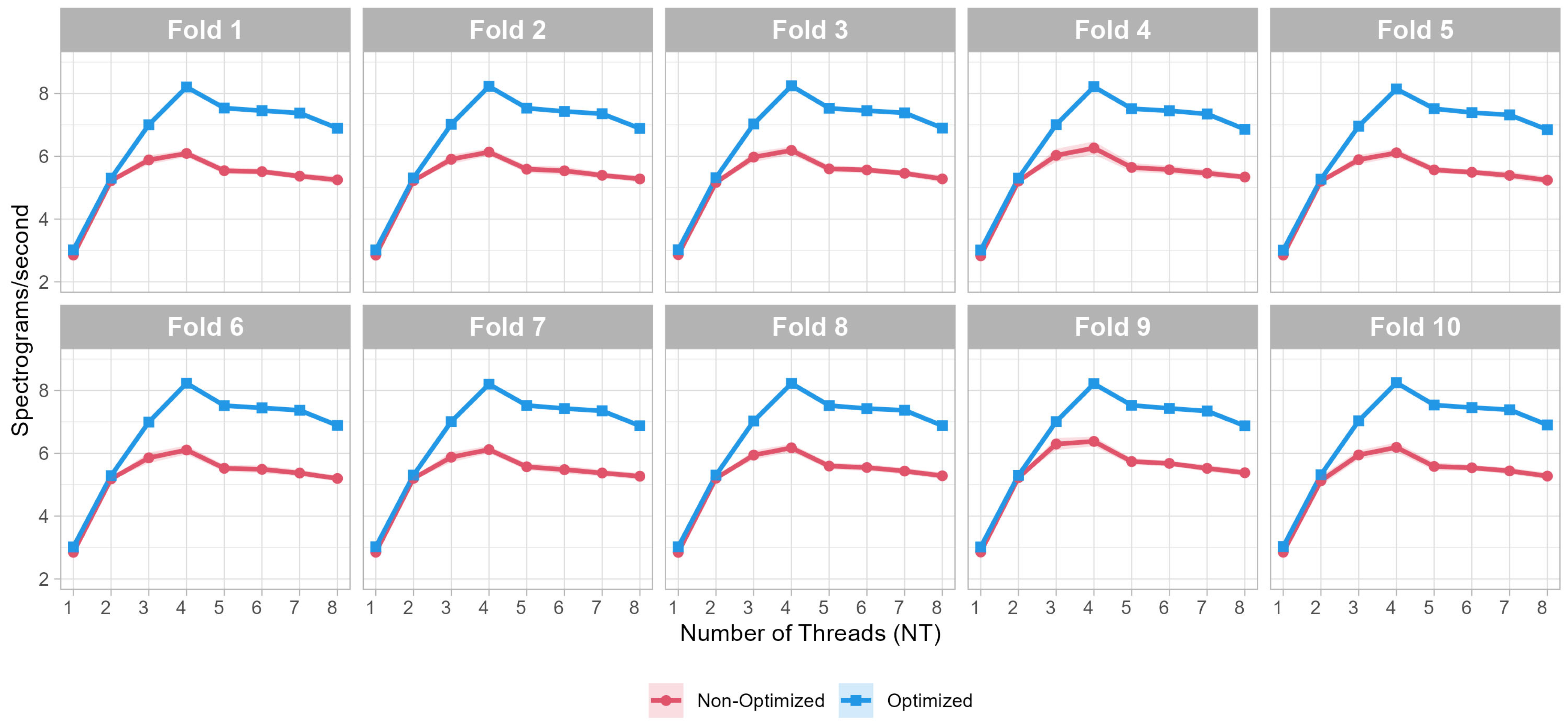
To further analyze the scalability of inference execution, we applied Amdahl’s Law to estimate the theoretical speedup achievable through parallelization. The maximum observed throughput (8.2 spectrograms/second) occurred when the number of threads (NT) is equal to 4, aligning with the quad-core architecture of the RPi Zero 2 W. Beyond this point, performance gains plateaued due to thread contention and memory bandwidth limitations, highlighting the diminishing returns of over-parallelization. Amdahl’s formula is given by the following:

$$S={\displaystyle \frac{1}{\left(1-P\right)+\frac{P}{N}}}$$

(2)

where S represents the theoretical speedup, P the parallelizable fraction of the computation, and N the number of threads.

3. Results

3.1. CNN Performance Comparison

The average (±standard deviation, SD) signal-to-noise ratio (SNR) over all the analyzed whistles is 11.9 ± 7.3 dB. The high standard deviation, which is nearly comparable to the mean value, indicates a significant variability in the SNR throughout the recording, thus suggesting the presence of both high- and low-quality whistles in the dataset. Optimized and non-optimized models generated via the 10-fold approach were evaluated using the common dataset comprising 1646 spectrograms (50% positive and 50% negative). Each configuration underwent ten repeated tests, with the same results across all iterations. Both the non-optimized and optimized versions exhibit performances comparable with those provided by the original TensorFlow model, if not slightly improved, as reported in

Table 1. Performance comparison of the original, non-optimized, and optimized models.

	Original Model				Non-Optimized Model				Optimized Model
Fold	Acc. %	Prec. %	Recall %	F1 %	Acc. %	Prec. %	Recall %	F1 %	Acc. %	Prec. %	Recall %	F1 %
1	86.0	91.6	79.2	85.0	86.3	92.4	79.2	85.3	86.3	91.9	79.7	85.4
2	89.0	94.1	83.2	88.3	89.6	95.3	83.2	88.8	89.4	95.4	82.9	88.7
3	83.0	86.8	77.8	82.1	84.2	89.3	77.8	83.1	84.4	87.5	80.2	83.7
4	84.8	88.6	79.7	83.9	86.0	91.2	79.7	85.1	86.1	91.4	79.7	85.1
5	84.9	88.5	80.3	84.2	85.8	90.3	80.3	85.0	85.9	90.4	80.3	85.1
6	87.8	93.8	81.0	87.0	88.9	96.1	81.0	87.9	88.9	96.1	81.0	87.9
7	90.2	95.0	84.8	89.6	90.8	96.3	84.8	90.2	90.7	96.1	84.8	90.1
8	86.4	90.9	80.9	85.6	87.7	93.7	80.9	86.8	87.7	93.7	80.9	86.8
9	89.9	94.3	84.8	89.3	90.3	95.2	84.8	89.7	90.3	95.2	84.9	89.8
10	87.8	93.8	81.0	87.0	88.0	94.2	81.0	87.1	87.7	94.0	80.6	86.8
mean	87.0	91.7	81.3	86.2	87.8	93.4	81.3	86.9	87.8	93.2	81.5	86.9
sd	2.4	2.9	2.3	2.5	2.1	2.5	2.3	2.3	2.1	2.8	2.0	2.2

.

3.2. Latency Analysis

The latency analysis performed on the ten-fold models highlights a clear relationship between inference time and the number of threads allocated to the TensorFlow Lite interpreter. As shown in Figure 3, when the NT is set to 1, the models exhibit the highest latency values, reaching approximately 300 ms for the non-optimized versions. Increasing the number of threads leads to a substantial reduction in inference time, with the most significant improvement occurring between NT = 1 and NT = 4. At NT = 4, the latency reaches its minimum, stabilizing around 120 ms for the optimized models and slightly less than 200 ms for the non-optimized models. Beyond this point, increasing the number of threads further results in a slight performance deterioration, as the latency starts to grow, although it remains widely lower than that at NT = 1. This trend suggests that the hardware, specifically the quad-core architecture of the RPi Zero 2 W, reaches its optimal performance when fully utilizing its four available cores.

The similar performance metrics across the TensorFlow, non-optimized TensorFlow Lite (TFLite), and optimized TFLite models suggest that the conversion process preserves model efficacy while enabling deployment on embedded systems. Although TFLite conversion may marginally degrade performance due to architectural constraints (e.g., quantization), it cannot inherently enhance predictive performance. Notably, the size reduction (37.5 MB for non-optimized TFLite; 9 MB for optimized TFLite) underscores the practical utility of TFLite for edge deployment.

3.3. Throughput and Resource Utilization Under Stress Conditions

While latency ideally measures the ability of the embedded system to process a single image with the CNN, continuous dolphin monitoring requires evaluating throughput and resource utilization over time to prevent potential bottlenecks or system overload. To assess the device’s response under varying computational demands, ten-fold models (both optimized and non-optimized) were tested on a dataset comprising 1636 images while the number of threads allocated to the TFLite interpreter was systematically varied from one to eight. Each test was repeated ten times to ensure statistical robustness. Given that a single test cycle required an average runtime exceeding six hours, the RPi Zero 2 W used in these experiments operated continuously for over 120 h without experiencing system crashes, functional anomalies, or performance degradation. The experimental results (Figure 4) clearly show better performance of the optimized models in terms of throughput and stability. In all the tested configurations, the optimized models consistently achieve a greater number of processed spectrograms per second compared to the non-optimized ones. Notably, the most significant performance gain occurs when increasing the number of threads from NT = 1 to NT = 2, where the throughput nearly doubles.

This behavior is observed across all folds, indicating that parallel execution significantly benefits inference speed, particularly in the optimized version. Beyond NT = 2, the optimized models maintain a steady and efficient processing rate, reaching more than 8 spectrograms per second, whereas the non-optimized models plateau at approximately 6 spectrograms per second. Then, both throughput curves decreased. Variations in workload distribution across the different folds could be evaluated in Table S2 of the Supplementary Materials. This suggests that optimization not only improves processing speed but also contributes to more predictable performance and better resource utilization.

3.4. CPU Usage and Temperature Under Stress Computing Tests

The CPU’s behavior, specifically its load and temperature, was monitored throughout the tests. Data were collected every 100 milliseconds and then aggregated into one-second intervals for analysis. Since no significant variations were detected, the results from the 10-fold models were combined into a single dataset. The key factor influencing CPU load variation is the number of threads used to execute the TFLite interpreter. The results in Figure 5 highlight an evident trend in CPU utilization and thermal performance as the number of threads increases. Detailed results are reported in

Table 2. (a) Average CPU load (%) for each number of threads (NT). (b) Average CPU temperature (°C) for each number of threads (NT) *.

(a)
Model	NT = 1	NT = 2	NT = 3	NT = 4	NT = 5	NT = 6	NT = 7	NT = 8
Non-optimized	100.4 ± 6.1	199.4 ± 16.7	298.3 ± 27.8	395.5 ± 39.2	393.6 ± 36.7	393.8 ± 36.1	390.8 ± 36.1	395.6 ± 36.1
Optimized	100.7 ± 4.5	182.5 ± 11.6	251.3 ± 19.8	314.4 ± 23.9	310.7 ± 24.2	311.8 ± 25.4	314.0 ± 24.1	315.7 ± 23.4
(b)
Model	NT = 1	NT = 2	NT = 3	NT = 4	NT = 5	NT = 6	NT = 7	NT = 8
Non-optimized	60.0 ± 2.3	76.2 ± 3.0	81.9 ± 1.2	83.4 ± 1.0	83.1 ± 1.0	83.1 ± 1.0	83.0 ± 1.0	82.8 ± 1.0
Optimized	51.2 ± 2.5	61.1 ± 2.3	69.5 ± 2.3	76.3 ± 2.4	75.6 ± 1.8	75.5 ± 1.8	75.6 ± 1.8	75.0 ± 1.7

* A detailed table is available in the Supplementary Materials.

a for CPU load and in Table 2b for CPU temperature.

The non-optimized model (in red with circles) rapidly saturates CPU resources, reaching a load of approximately 400% from NT = 4 onwards, with significant variability. In contrast, the optimized model (in blue with squares) exhibits a more controlled increase, peaking at ≈315% CPU load at NT = 8. The wide variability in CPU load observed in the unoptimized model is primarily due to the performance of the CNN, which can vary in computational demand depending on the complexity and size (in kB) of the input image. This phenomenon can be verified by running the scripts described in the Data Availability Statement Section and provided in [24].

In terms of thermal behavior, the optimized model maintains a significantly lower CPU temperature across all thread configurations. The non-optimized model exceeds 80 °C from NT = 4 onwards, operating near critical thermal thresholds. On the other hand, the optimized model remains within safer limits, stabilizing at approximately 75–76 °C. This suggests a reduced risk of thermal throttling, contributing to better system stability and reliability during continuous inference operations.

3.5. Memory Usage Analysis

Memory usage analysis revealed that the volume used is stable when the models and the number of threads with which the CNN is executed vary. Even when changing the number of spectrograms used in the test (in blocks of 1, 5, 50, 250), no variations are observed in the amount of memory used (

Table 3. Average memory consumption (MB) across different inference phases for optimized and non-optimized models.

Component	NT = 1	NT = 2	NT = 3	NT = 4	NT = 5	NT = 6	NT = 7	NT = 8
Non-optimized
Python environment	35.13	35.13	35.12	35.13	35.14	35.14	35.12	35.12
Model load	37.74	37.73	37.74	37.75	37.73	37.74	37.73	37.75
Tensor allocation	51.52	51.43	51.38	51.37	51.29	51.30	51.33	51.32
Inference increment	0.00	0.00	0.00	0.00	0.00	0.00	0.00	0.00
Cumulated	124.39	124.28	124.24	124.25	124.16	124.18	124.18	124.19
Optimized
Python environment	35.16	35.16	35.16	35.15	35.15	35.15	35.15	35.15
Model load	10.88	10.88	10.87	10.88	10.87	10.88	10.87	10.88
Tensor allocation	29.35	29.21	29.16	29.19	29.22	29.23	29.25	29.26
Inference increment	3.06	3.05	3.06	3.09	3.08	3.09	3.08	3.11
Cumulated	78.45	78.30	78.25	78.30	78.32	78.34	78.35	78.38

).

Model optimization reduced cumulative memory consumption by 37%, from 124.39 MB to 78.45 MB, primarily due to a 71% reduction in model size (37.74 MB to 10.88 MB) and a 43% decrease in tensor allocation overhead (51.52 MB to 29.35 MB). The optimized models also demonstrated excellent scalability, with memory usage remaining stable across thread configurations (NT = 1 to NT = 8) and inference overhead increasing by only 1.6% (3.06 MB to 3.11 MB).

3.6. Parallelization Limits According to Amdahl’s Law

Computational advantage resulting from the use of more than one thread has been verified by applying Amdahl’s Law to calculate the speedup, normalized to the best performance achieved with NT = 4 as in Equation (3):

$$S_{obtained}={\displaystyle \frac{Throughput at NT=4}{Throughput at NT=1}}={\displaystyle \frac{8.2}{3.0}}\approx 2.73$$

(3)

Rearranging the Amdahl Equation (2), we obtain that 85% of the inference pipeline is parallelizable, while 15% remains sequential.

Table 4. Comparison between observed and theoretical throughput based on Amdahl’s Law.

NT	Theoretical Speedup	Theoretical Throughput (Item/s)	Observed Throughput (Item/s)
1	1	3	3
2	1.67	5.01	5.3
3	2.11	6.33	7
4	2.73	8.19	8.2
5	3.07	9.21	7.5
6	3.33	9.99	7.4
7	3.54	10.62	7.4
8	3.7	11.1	6.9

illustrates the alignment between theoretical and observed throughput up to NT = 4, beyond which performance degrades due to hardware limitations. This confirms that the quad-core architecture reaches its optimal efficiency when fully utilizing its four cores, while exceeding this threshold leads to increased contention and lower efficiency.

4. Discussion

The experimental activity conducted has comprehensively demonstrated the computational advantages of employing optimization techniques in converting TensorFlow models to TFLite, as well as the suitability of the Raspberry Pi Zero 2 W to handle the associated workload. The following sections provide a detailed analysis of the various aspects examined. Above all, it is relevant to underline that the CNN model can recognize a single whistle even in the challenging conditions of the present dataset, including situations where multiple dolphins vocalize simultaneously, resulting in overlapping whistles that may have different shapes and durations. The dataset used in this study, indeed, is characterized by high variability due to the concomitant presence of more dolphins, as well as the occurrence of other types of vocalizations such as echolocation clicks and burst pulse sounds. Nevertheless, the present model showed encouraging outcomes (Table 1). Moreover, the performance metrics are comparable in TF and TFLite implementations, supporting the robustness of the TFLite approach.

4.1. Scalability and Computational Efficiency

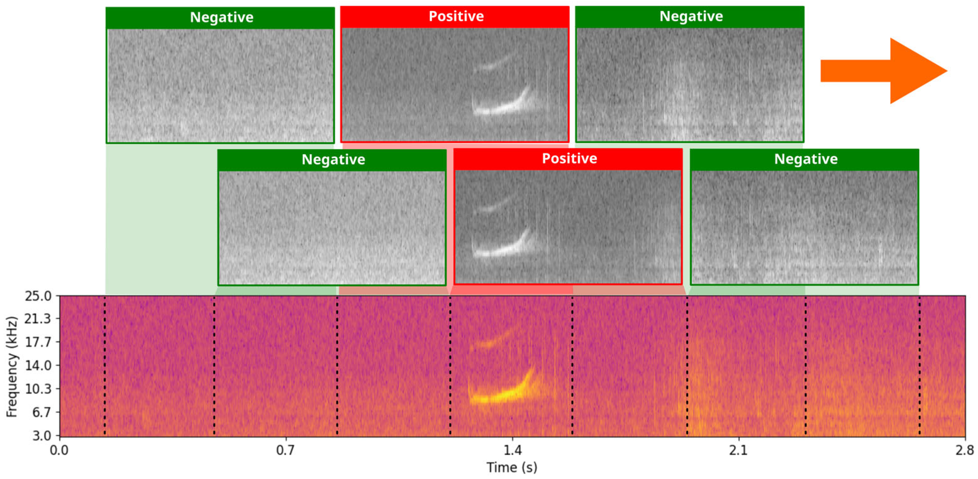
Raspberry Pi boards, including the zero variant, have already been utilized in CNN-based applications [25]. Nevertheless, their deployment for real-time dolphin whistle detection has never been previously considered since it poses unique challenges because of the high-throughput processing requirements of spectrogram analysis. The detection design—based on 0.8 s audio segments with 50% overlap—necessitates the continuous processing of 2.5 spectrograms per second to maintain temporal resolution, thereby demanding stringent latency and resource management. Figure 6 illustrates the sequential segmentation and processing workflow, demonstrating how the model efficiently divides the incoming audio stream into overlapping windows to achieve continuous detection while adhering to the hardware constraints of the Raspberry Pi. Results demonstrate that optimization significantly enhances inference speed while maintaining accuracy, enabling real-time whistle detection.

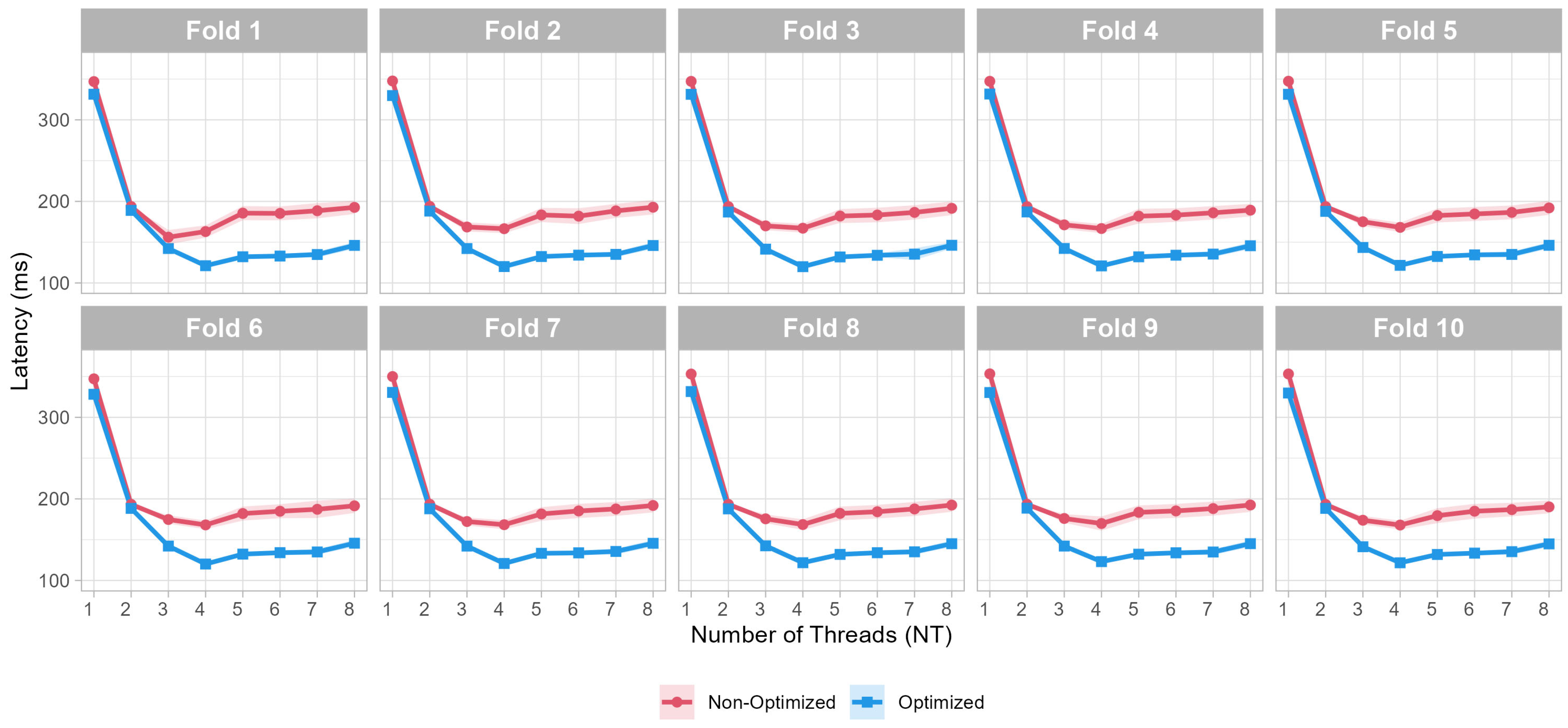
To assess the computational efficiency of the optimized CNN, we evaluated both latency and throughput across different thread configurations. Results indicate that model optimization reduces the inference time by approximately 40% (120 ms vs. 200 ms at NT = 4), significantly increasing processing capacity. Additionally, the optimized model demonstrates improved memory efficiency, reducing RAM utilization by 37% compared to the non-optimized version.

4.2. System Resource Management

Overall, the tested configuration reserves sufficient resources for concurrent tasks such as audio sampling and preprocessing, a decisive advantage over always-active pingers. From this perspective, Raspberry Pi Zero 2 W’s 512 MB RAM proved more than adequate, with memory usage never exceeding 16% of capacity with the optimized model (25% with no optimization). A critical observation from testing non-optimized models revealed significant thermal throttling effects when deploying these models with thread counts exceeding 3. This phenomenon, documented in the device references [26], occurs when the CPU temperature surpasses the critical threshold of 80 °C, triggering computational capacity reduction and measurable throughput degradation. Thermal management becomes essential under high computational loads, particularly when aggregate CPU utilization exceeds 200% (indicative of saturation across more than two cores), necessitating robust heat dissipation solutions. Experimental results demonstrated that limiting thread counts to two during sustained CNN inference tasks effectively mitigates thermal stress. In optimized models, this configuration maintained CPU temperatures below 65 °C, ensuring operational stability within safe thermal margins. Although power consumption aspects were not explored in detail in this work, they will be addressed in future publications that will also examine the energy cost of the audio acquisition board.

4.3. Main Contributions of the Present Work

To facilitate the comprehension of the impact of the present study, this paragraph outlines the main contributions and innovations introduced by this work. In this paper, we detail a targeted TinyML solution for real-time dolphin whistle detection on ultra-low-cost hardware. The main contributions are as follows:

• On-device CNN inference with TFLite: Deployment of a convolutional neural network (originally trained in TensorFlow) on a Raspberry Pi Zero 2 W using TensorFlow Lite, allowing real-time classification in a resource-constrained environment.
• Maintained classification performance with drastic model compression: Through post-training optimization, we reduce the model size by 76% (from 37.5 MB to 9 MB) while preserving key metrics (Accuracy: 87.0% vs. 87.8%; F1-score: 86.2% vs. 86.9%), validating our approach for TinyML-driven edge applications.
• Substantial latency reduction: By tuning the TFLite interpreter’s thread allocation, we halve inference time—from ~200 ms to ~120 ms at the optimal four-thread configuration—thus meeting the strict temporal requirements for 0.8 s whistle events.
• Comprehensive resource and thermal profiling: Detailed evaluation of throughput, memory footprint, CPU load, and thermal behavior under continuous stress tests (120 h of uninterrupted operation), highlighting the Raspberry Pi Zero 2 W’s suitability for sustained, real-time acoustic monitoring.
• A modular architectural framework for marine deterrent systems: Results of this work can be integrated into an end-to-end pipeline—spanning real-time DSP preprocessing, spectrogram generation, CNN inference, event logging, and deterrent sound emission—laying the groundwork for a scalable, low-cost interactive acoustic deterrent platform.

4.4. Limitations, Future Improvements, and Deployment Challenges

Despite the encouraging results achieved in this study, we must acknowledge that it presents certain limitations. The model was trained and tested on data acquired from bottlenose dolphins residing in a marine park setting, thus reflecting the specific acoustic and environmental conditions of that controlled habitat. Differences among individuals and across species, as well as shifts in environmental open-sea parameters and background noise, are likely to affect the model’s generalization capacity. These sources of variability may introduce distortions in the input data, thereby impairing model performance. To address such limitations, applying targeted preprocessing techniques—either at the audio signal level or directly to spectrogram representations—could facilitate the separation of individual vocalizations from extraneous acoustic content, thus improving classification accuracy. Ongoing research will aim to identify the most effective digital signal processing methods for mitigating both ambient noise and overlapping vocal elements.

Moreover, the present study employs a CNN trained on dolphin whistles collected in controlled environments, yielding methodologically promising results. At the moment, the current work intentionally leverages an existing TensorFlow-based CNN to prioritize comparative benchmarking on a single-board computer. However, the methodological framework presented here can be adapted to other dolphins’ vocalizations and cetacean species by retraining the model with species-specific datasets.

The proposed system’s practicality is further enhanced when integrated with four complementary components: a low-cost hydrophone already presented in a previous study of the same authors of this article [11], on-device audio acquisition, spectrogram generation using optimized FFT libraries, and a deterrence mechanism based on programmable acoustic deterrents triggered by real-time detections.

Future efforts should focus on developing multi-class CNNs trained on open-sea recordings to enhance ecological relevance and generalizability. A critical future challenge lies in further miniaturizing the system for deployment on ultra-low-power devices like the ESP32. However, two key barriers persist:

• The need for significantly smaller CNN architectures (current model: 9 MB) to accommodate MCU memory constraints;
• The absence of robust solutions for high-fidelity audio sampling at 192 kS/s, which is a prerequisite for analyzing cetacean impulsive sounds, which can exceed 160 kHz in frequency.

Furthermore, we plan to validate the system in field deployments, evaluating performance under real oceanic conditions. This will enable testing in the presence of variable background noise, multiple cetacean species, and anthropogenic acoustic interference.

5. Conclusions

The present study indicates that a Raspberry Pi Zero 2 W represents a viable platform for deploying TensorFlow Lite-optimized convolutional neural networks (CNNs) trained to recognize bottlenose dolphin whistles, achieving performance metrics comparable to standard computing systems.

Experimental results confirm the device’s capacity to execute real-time inference tasks with latencies below 200 ms and throughput exceeding 5 spectrograms per second, even using the safest two-thread configurations. These benchmarks hold for both baseline and optimized TFLite models, though optimization confers significant advantages in resource efficiency and operational stability.

Optimized models exhibit the following systemic improvements across critical parameters:

• Computational load: Reduced CPU utilization (18–25% lower than non-optimized counterparts) due to operator fusion and quantized arithmetic.
• Memory footprint: 45–60% compression in model weights through post-training quantization.
• Thermal profile: Sustained operation below 65 °C at two-thread configurations, avoiding thermal throttling thresholds.
• Performance: Latency improvements (reduced by 16–20%) and throughput gains of 12–20% compared to non-optimized models.

Future enhancements could focus on the adoption of marine-specific datasets and multi-class classifiers to distinguish between bottlenose dolphins, other cetaceans, and anthropogenic noise.