Optimization of Q and R Matrices with Genetic Algorithms to Reduce Oscillations in a Rotary Flexible Link System

Abstract

Automatic control of robots with flexible links has been a pivotal subject in control engineering and robotics due to the challenges posed by vibrations during repetitive movements. These vibrations affect the system’s performance and accuracy, potentially causing errors, wear, and failures. LQR control is a common technique for vibration control, but determining the optimal weight matrices [Q] and [R] is a complex and crucial task. This paper proposes a methodology based on genetic algorithms to define the [Q] and [R] matrices according to design requirements. MATLAB and Simulink, along with data provided by Quanser, will be used to model and evaluate the performance of the proposed approach. The process will include testing and iterative adjustments to optimize performance. The work aims to improve the control of robots with flexible links, offering a methodology that allows for the design of LQR control under the design requirements of controllers used in classical control through the use of genetic algorithms.

1. Introduction

In robotics, particularly in systems incorporating flexible links, effective vibration management is essential for maintaining system precision and stability. Flexible links are highly valued in the field of robotics for their capacity to enhance the accuracy in the transmission of motion and forces, and for their utility in passive vibration reduction [1]. In addition, Flexible-link robots present several advantages over their rigid counterparts, mainly due to their lightweight construction, which leads to high throughput and low power consumption [2], although passive reduction methods are effective under certain conditions, they exhibit limitations in dynamic environments where the demands for responsiveness and adaptability intensify. In contrast, active control systems can provide superior adaptability and precision by dynamically adjusting control parameters in response to real-time environmental conditions. This is particularly relevant in advanced robotics applications where even minor deviations can lead to significant errors or system failures. Therefore, the integration of active control strategies emerges as a critical solution to overcome the limitations of purely passive isolation methods in robots with flexible components.

Active control of robots with flexible links has been a topic of significant importance in control engineering and robotics [3]. On one hand, flexible links present an engineering challenge due to the vibrations that occur during the transitional phase of controlling the position of a robotic arm, affecting both the performance and the precision of the system [4]. The issues arising from these vibrations range from positioning errors to component wear, and occasionally, system failures. On the other hand, studies such as [5] investigate how micro-positioning systems, which utilize flexibility based on the elastic deformation of joints or mechanism sections, eliminate wear, noise, and friction. These characteristics are crucial when considering the automation of robots with flexible links in environments that demand high precision, such as in surgical robotics or micro-device manufacturing. The discussion includes the use of active control systems, deliberating on the design of controllers and actuators and the selection of essential materials for precision. Cases like these motivate the pursuit of better techniques that effectively address the ability to control these vibrations according to the system’s requirements.

The linear quadratic regulator (LQR) is one of the most common and effective approaches in controller design, given its ability to provide good performance based on quadratic criteria. In LQR control, the performance index is minimized with optimal weight matrices. The [Q] and [R] matrices are the most crucial parameters to keep actuator voltage within certain limits while maintaining maximum control performance. Hence, the importance in LQR control lies in determining the optimal state weighting matrix [Q] and the input weighting matrix [R] [6].

In advanced control systems, proper design and tuning of controllers are essential to ensure the desired system performance; however, the appropriate choice of weighting matrices in LQR design is crucial and can be complex in many situations. Optimizing these matrices can be challenging, as manual selection or the use of traditional optimization techniques may not always yield the best results, especially in complex or nonlinear systems. To overcome this challenge, this study proposes the use of genetic algorithms as in [7] to find the weights for the gain matrix K according to the controller design requirements.

In [8], optimization deals with performance criteria such as rise time, overshoot, control energy, and a measure of robustness, among others. Optimization is achieved through the use of an elitism-based genetic algorithm (GA). Also, Ref. [9] investigates dynamic modeling and vibration control for a large flexible space truss. The space truss is a typical periodic triangular prism structure consisting of beams and rods. Considering the transverse deformation of the entire structure, the equivalent dynamic model of the space truss is established using the principle of energy equivalence. Fourth-order governing equations of the equivalent cantilever beam model are derived and solved by adopting Hamilton’s principle and the Galerkin method to achieve its discrete dynamic model. The LQR vibration controller is designed when the space truss is subjected to periodic and impulse excitation. The control moment is applied to the large-scale finite element model of the space truss, and numerical simulations prove the effectiveness of the designed LQR vibration controller for the suppression of vibrations.

In [10], the so-called linear quadratic regulation problem is a modern control strategy that, through the configuration of the weight matrices Q and R, takes on the tedious task traditionally performed by specialists in controller optimization, finding the control parameters that minimize unwanted deviations. However, there are no simple analytical methods that assist the designer in defining the values of these matrices, which depend on the system, the control to be achieved, and the efforts of the control variables, making deep knowledge of the process essential for the engineer. Classic approaches such as trial and error, Bryson’s method, and pole placement are tedious and do not guarantee the expected performance. This research proposed a methodology based on genetic algorithms and particle swarm optimization to define the weight matrices Q and R, achieving the design of optimal controllers in a simple, fast manner starting from basic knowledge of the system to be controlled. The controller is evaluated using MATLAB and Simulink, assessing the effectiveness of the proposed scheme in terms of tracking and robustness through three test cases.

Our research is conducted on a cantilever beam, which is attached to a DC motor, and the model representation is executed in state space. The model is compared with the actual plant (rotary flexible link) with data provided by Quanser^®, a global leader in hardware for real-time control design in education and research [11], where the GA-LQR controller is evaluated. This work highlights the genetic algorithm used for the optimization of a LQR under specific designer conditions swiftly and effectively in robots with flexible links, aiming to minimize oscillations at the tip of the link by controlling its base.

The primary contributions of this research include the development of a GA-LQR controller that integrates classic control design criteria, such as percentage overshoot and settling time [12], directly into the algorithm’s cost function, allowing for precise alignment of the Q and R parameters with the specific design objectives of the controller. The results of the simulations clearly confirm that the proposed control system effectively minimizes the end vibrations of the manipulator, fulfilling the requirements set out in the design of the genetic algorithm. Moreover, a general methodology has been established for enforcing specific design requirements for position control of the tip of a rotating flexible link, using genetic algorithm techniques over a LQR for the optimization of desired parameters.

The use of a reference model for the GA ensures that the resulting parameters are aligned with a known desired behavior, although it is essential that the reference model be representative enough of the real system for the optimized parameters to be effective in practice. For future work, the challenge of using the GA-LQR control in real time is proposed. One approach could consider running the GA on a slower cycle, which allows for reviewing and adjusting the LQR parameters based on the system’s recent performance, while a faster LQR controller handles real-time control. Additionally, an improvement would be to develop a faster and more efficient version of the GA that can operate in real time or near-real time. It is hoped that this proposal will contribute to the scientific and technological community by offering other perspectives to develop controllers for flexible systems. Furthermore, this approach may serve as a foundation for future research and applications in the industry.

2. Modeling of the Rotary Flexible Link System

For the evaluation of the control technique GA-LQR, modeling is conducted both theoretically and experimentally. The theoretical modeling is divided into two parts: mechanical and electrical. The Lagrange method is used to find the motion equation of the system. These equations describe the movement of the mechanism in relation to a voltage applied to the servo motor. For the modeling through system identification, data from [13] are acquired, specifically a rotary flexible link system provided by QUANSER^®, through its software “Quanser Interactive Labs”, version 2.15, which offers academically appropriate and high-fidelity laboratory experiences through interactions with virtual hardware. The rotary flexible link (RFL) module has facilitated the evaluation of control over the developed model. The system has been designed to couple with a rotary servo. The module simulates real-world problems in flexible and lightweight structures, being essential for studying vibration control, resonance, and modeling in robots or spacecraft [14]. The mathematical model is obtained in a state-space representation; the following is a detailed account of the model.

An usual modeling method for flexible systems is to approximatively describe the dynamics of the flexible link with finite number modes [14]. Nevertheless, another modeling method considers entire modes of flexible structures. Dynamic models, including the infinite-dimensional governing equation and boundary conditions, are established to describe the dynamic behaviour of the flexible manipulators via Hamilton’s principle [15].

For the analysis of the link, the Euler–Bernoulli theory is used, which considers the link as a bar subjected to lateral vibrations. To derive the model’s equations, Hamilton’s principle is applied. The bar contributes to both the kinetic and potential energy of the system, while the base contributes only to the kinetic energy.

In accordance with the literature from [3], the robot with flexibility in a single-degree-of-freedom link consists of a flexible link that is connected to a base. On the base, a motor is present, which applies torque to the link to move it to the desired position. The motion of the link is horizontal; thus, gravitational forces are not considered. The primary objective of control is to minimize the deflection as much as possible.

Figure 1 illustrates the reference frame used to define the variables related to the robot. The length of the link is denoted by l, the torque by $\tau$, the time variable by t, the deflection of the link relative to the neutral axis by $\alpha (x,t)$, the coordinate along the neutral axis of the link by x, and $\theta \left(t\right)$, which is the rotation angle of the link’s axis relative to the neutral axis (rigid line).

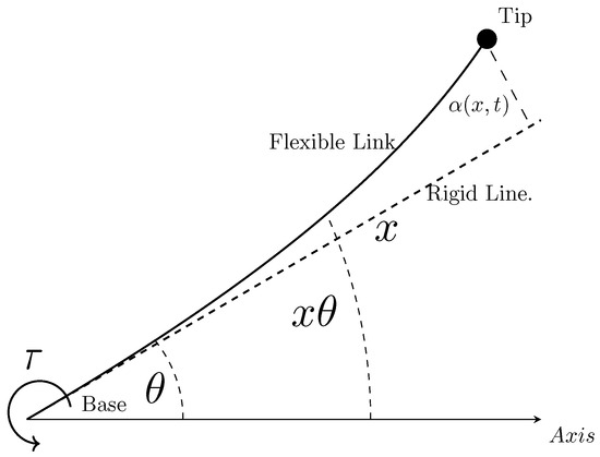
Figure 1. Representation of the flexible link manipulator.

The link is characterized as a bar subjected to external forces distributed along its entire length. The theories used in the description of the vibrations of a bar include those of Euler–Bernoulli, Rayleigh, and Timoshenko. The simplest theory of lateral vibration is that of Euler–Bernoulli [16].

Based on the Euler–Bernoulli theory, the link is modeled. In this theory, second- and higher-degree terms in the deformation variables are neglected, and the following assumptions are considered:

• The link is a bar with uniform geometric characteristics and a uniform mass distribution. This assumption implies that the deflection of a section through the link is due only to bending or deflection and not to shear. Moreover, the contribution of the rotational inertia of the link section to the total energy is negligible.
• The link is flexible in the lateral direction, with only elastic deformations being present. This assumption is reinforced by the mechanical construction of an actual flexible arm.
• Nonlinear deformations as well as internal friction or other external disturbances are negligible.

Applying this theory, the link is a bar of length l, the cross-sectional area of the bar is denoted by $A_T$, $\rho$ is the mass density acting on an external force $q(x,t)$ in the z direction, $I_h$ is the axial inertia, and E is Young’s modulus.

It is assumed that the cross section at a distance x remains plane even after bending and has a rotation through the y-axis given by the slope ${\alpha }^{\prime }$ of the elastic curve. The displacements of the bar can then be defined as:

$$\begin{array}{cc}\hfill u_x& =-z{\alpha }^{\prime }(x,t)\hfill \end{array}$$

(1)

$$\begin{array}{cc}\hfill u_y& =0\hfill \end{array}$$

(2)

$$\begin{array}{cc}\hfill u_z& =\alpha (x,t)\hfill \end{array}$$

(3)

The strain is given by ${\epsilon }_{xx}=z{\alpha }^{″}(x,t)$. The stress is given by ${\tau }_{xx}=-Ez{\alpha }^{″}(x,t)$.

Note: In the equations, a comma on top represents differentiation with respect to x, and a dot represents differentiation with respect to time.

To apply Hamilton’s principle, both the kinetic and potential energies of the robot are required. The first is constituted by the contributions from the link and the base. The second, the potential energy, depends entirely on the link.

From Figure 1, $O-Axis$ is the neutral axis when the arm is rigid. The displacement of any point P across the neutral axis at any distance from the axis (not exceeding the length of the bar) is given by the angle of the axis $\theta \left(t\right)$ and the deflection $\alpha (x,t)$ measured from the line $O-Axis$. This displacement is expressed as follows:

$$y(x,t)=\alpha (x,t)+x\theta \left(t\right)$$

(4)

The potential energy (due to deformation) is given by:

$$U=\frac{1}{2}{\int }_0^l{\int }_{A}E{z}^2{\alpha }^{″}(x,t)dAdx=\frac{1}{2}{\int }_0^{l}EI{\left({\alpha }^{″}(x,t)\right)}^{2}dx$$

(5)

From Figure 1, the absolute position of a point along the link is described by [15]:

$$p=\left(\begin{array}{c}{p}_x\\ p_y\end{array}\right)=\left(\begin{array}{c}xcos\theta \left(t\right)-\alpha (x,t)sin\theta \left(t\right)\\ xsin\theta \left(t\right)+\alpha (x,t)cos\theta \left(t\right)\end{array}\right)$$

(6)

Since the link is fixed to the base, the following boundary geometric conditions are satisfied:

$$\alpha (0,t)={\alpha }^{\prime }(0,t)=0$$

(7)

The kinetic energy is given by:

$$T=T_h+T_l$$

(8)

where the kinetic energy of the axis is given by:

$$T_h=\frac{1}{2}{I}_h\dot{\theta }{\left(t\right)}^2$$

(9)

where $I_h$ is the moment of inertia of the link, and $T_l$ is the disregarding axial inertia due to ${\dot{u}}_x$, described by:

$$T_l=\frac{1}{2}\rho {\int }_0^l({\dot{p_x}}^2+{\dot{p_y}}^2)dx=\frac{1}{2}\rho {\int }_0^l\left(x^2\dot{\theta }{\left(t\right)}^2+2x\dot{\theta }\left(t\right)\dot{\alpha }(x,t)+{\dot{\alpha }}^2(x,t)\right)dx$$

(10)

The non conservative work for the input torque $\tau$ can be written as:

$$W=\tau \theta$$

(11)

To obtain the equations of motion of the manipulator, Hamilton’s extended principle, described by [17].

$${\int }_{t_1}^{t_2}(\delta L+\delta W)dt=0$$

(12)

can be used, subject to $\delta \theta =\delta u=0$ at $t_1$ to $t_2$, where $t_1$ and $t_2$ are two arbitrary times ($t_1<t_2$) and $L=E_k-E_p$ is the system’s Lagrangian.

$\delta W$ represents the virtual work, $\delta \theta$ represents a virtual rotation and $\delta u$ represents a virtual elastic displacement [18]. Using (5), (10) and (11) the integral in (12) can be written as:

$${\int }_{t_1}^{t_2}(\delta T\left(t\right)-\delta U\left(t\right)+\delta W\left(t\right))dt=0$$

(13)

where $\delta W\left(t\right)=u\left(t\right)\delta \theta \left(t\right)$ represents the virtual work performed by the torque. The rotary inertia and shear deformation are more pronounced at high frequencies and more influential on the higher modes [19]. Since investigations have shown that the first two modes are sufficient in modelling the manipulator, the rotary inertia and shear deformation effects can be ignored [18].

To determine $\delta T\left(t\right)$, consider the functional:

$$T\left[\theta \left(t\right)\right]={\int }_{t_1}^{t_2}F(t,\theta \left(t\right),\dot{\theta }\left(t\right))dt$$

(14)

Applying the general Euler equation, one obtains:

$$\delta T\left(t\right)=\left[I_h\dot{\theta }+\rho {\int }_0^l(x^2\ddot{\theta }{\left(t\right)}^2+{\alpha }^2\ddot{\theta }\left(t\right)+x{\ddot{\alpha }}^2(x,t))dx\right]\delta \theta +\left[\rho {\int }_0^l\left(\ddot{\alpha }(x,t)\right)+x\ddot{\theta }\left(t\right))dx\right]\delta \alpha$$

(15)

The deformation $\alpha (x,t)$ is considered to be very small in comparison to the length of the link. That is, $\alpha (x,t)\le 0.1l$. See the article by Cannon [20].

By neglecting the term involving $\alpha {(x,t)}^2$, and grouping the terms in $\delta \theta$, one obtains.

$$I_h\ddot{\theta }+\rho {\int }_0^l(x^2\ddot{\theta }\left(t\right)+x\dot{\alpha }(x,t))dx=u$$

(16)

From the functional:

$$U\left[\alpha (x,t)\right]=\frac{1}{2}{\int }_0^l{\alpha }^{″}{(x,t)}^{2}dx$$

(17)

the variation $\delta U$ is calculated, which is given by the expression:

$$\delta U={\int }_0^l{\alpha }^{″}(x,t)\delta {\alpha }^{″}(x,t)dx$$

(18)

If integrated by parts, it results in:

$$\delta U={\left[{\alpha }^{″}(x,t)\delta {\alpha }^{\prime }(x,t)\right]}_0^l-{\int }_0^l{\alpha }^{‴}(x,t)\delta {\alpha }^{\prime }(x,t)dx$$

(19)

Integrating again by parts, we obtain:

$$\delta U={\left[{\alpha }^{″}(x,t)\delta {\alpha }^{\prime }(x,t)\right]}_0^l-{\left[{\alpha }^{‴}(x,t)\delta \alpha (x,t)\right]}_0^l+{\int }_0^l{\alpha }^{″″}(x,t)\delta \alpha (x,t)dx$$

(20)

This expression must vanish at the extremal of the functional, that is,

$${\alpha }^{″}(0,t)=0;{\alpha }^{″}(l,t)=0$$

(21)

By grouping the terms involving $\delta \alpha$, one obtains

$$EI{\alpha }^{″″}(x,t)+\rho \ddot{\alpha }(x,t)+\rho x\ddot{\theta }\left(t\right)=0$$

(22)

With the corresponding boundary and initial conditions as:

$${\Sigma }_{RFE}:\left\{\begin{array}{c}\alpha (0,t)=0\hfill \\ I_h{\ddot{\alpha }}^{\prime }(0,t)-EI{\alpha }^{″}(0,t)=\tau \left(t\right)\hfill \\ M_p{\alpha }^{″}(l,t)-EI{\alpha }^{‴}(l,t)=0\hfill \\ I_p{\ddot{\alpha }}^{\prime }(l,t)+EI{\alpha }^{″}(l,t)=0\hfill \\ \alpha (x,0)=0\hfill \\ {\alpha }^{\prime }(x,0)=0\hfill \end{array}\right.$$

(23)

Substituting for $y(x,t)$ from (4) into (22) and (23) and simplifying yields the governing equation of motion of the manipulator in terms of $y(x,t)$ as:

$$EI{y}^{″″}(x,t)+\rho \ddot{y}(x,t)=0$$

(24)

with the corresponding boundary and initial conditions as:

$${\Sigma }_{RFE}:\left\{\begin{array}{c}y(0,t)=0\hfill \\ I_h{\ddot{y}}^{\prime }(0,t)-EI{y}^{″}(0,t)=\tau \left(t\right)\hfill \\ -EI{y}^{‴}(l,t)=0\hfill \\ I_p{\ddot{y}}^{\prime }(l,t)+EI{y}^{″}(l,t)=0\hfill \\ y(x,0)=0\hfill \\ y^{\prime }(x,0)=0\hfill \end{array}\right.$$

(25)

Equation (24) gives the fourth-order partial differential equation (PDE), which represents the dynamic equation describing the motion of the flexible manipulator [21].

Obtaining the Laplace transform of the system (24) and solving for the roots of the determinant of the matrix of coefficients, a series of natural vibrational modes of the system is obtained. In AMM, the link flexibility is represented by a combination of separable mode shapes and time-varying generalized coordinates. The modal series is truncated to a finite dimension because the contribution of higher modes to the overall movement is negligible, and dynamics of the system are dominantly governed by only the first few (low frequency) modes [18]. This method is usually adopted when the global shape functions can be analytically computed, like in the case of links with simple geometries [22].

Using the method of assumed modes [23], the variables of the system can be expressed as:

$$y(x,t)=\sum _{i=1}^{n_e}{\varphi }_i\left(x\right)q_i\left(t\right)$$

(26)

where the admissible function, ${\varphi }_i$, also called the mode shape, is purely a function of the displacement along the length of the manipulator and $q_i$ is purely a function of time and includes an arbitrary, multiplicative constant. The zeroth mode is the rigid-body mode of the manipulator, characterising the so-called rigid manipulator as considered without elastic deflection [21].

Substituting for $y(x,t)$ from (26) into (24) and manipulating yields two ordinary differential equations as:

$${\varphi }_i^{″″}\left(x\right)-{\beta }_i^4{\varphi }_i\left(x\right)=0,{\ddot{q}}_i\left(t\right)+{\omega }_i^2{q}_i\left(t\right)=0$$

(27)

where:

$${\omega }_i^2=\frac{EI}{\rho }{\beta }_i^4$$

(28)

where ${\beta }_i$ is a constant. Let two constants ${\lambda }_i$ and $ϵ$ be defined as:

$${\lambda }_i={\beta }_{i}l,ϵ=\frac{I_h}{M{l}^2}=\frac{3I_h}{I_b}$$

(29)

where $M=\rho l$ is the mass of the manipulator.

From the properties of self-adjoint systems, the mode shapes must also satisfy the orthogonality condition:

$${\int }_0^{l}EI{\varphi }_i^{″}\left(x\right){\varphi }_j^{″}\left(x\right)dx=I_T{\omega }_i^2{\delta }_{ij}$$

(30)

where ${\varphi }_i^{″}=\frac{d^2{\varphi }_i}{d{x}^2}$. The analytical values of natural frequencies ${\omega }_i$ can then be obtained using (29). $ϵ$ determines the vibration frequencies of the manipulator; a small $ϵ$ corresponds to the manipulator with lower vibration frequencies. For a very large $ϵ$, the vibration frequencies correspond to those of a cantilever beam. By considering the boundary conditions, the mode shape function ${\varphi }_i\left(x\right)$ of the manipulator can thus be obtained like a fourth-order ordinary differential equation with a solution on the form:

$${\varphi }_i\left(x\right)=A_{i}sin\left({\beta }_{i}x\right)+B_{i}sinh\left({\beta }_{i}x\right)+C_{i}cos\left({\beta }_{i}x\right)+D_{i}cosh\left({\beta }_{i}x\right)$$

(31)

In the absence of an external torque, (22) describes the behaviour of the manipulator in free transverse vibration with a solution $u(x,t)$ as:

$$u(x,t)=\sum _{i=1}^n{q}_i\left(t\right){\varphi }_i\left(x\right)\mathrm{for}i=1,2,\cdots ,n$$

(32)

The kinetic energy $E_k$ and potential energy $E_p$ of the system, in terms of the natural modes, can be obtained as [21]:

$$\begin{array}{cc}\hfill E_k& =\frac{1}{2}{\delta }_{ij}\sum _{i=1}^n{b}_i{q}_i^2\hfill \end{array}$$

(33)

$$\begin{array}{cc}\hfill E_p& =\frac{1}{2}\sum _{i=1}^n\sum _{j=1}^n{q}_i{q}_j{\int }_0^{l}EI{\varphi }_i^{″}\left(x\right){\varphi }_j^{″}\left(x\right)dx=\frac{1}{2}{\delta }_{ij}{I}_T\sum _{i=1}^n{\omega }_i^2{q}_i^2\hfill \end{array}$$

(34)

The dissipated energy $E_f$ and the work W can be obtained as:

$$E_f=\frac{1}{2}(I_h+I_b)\sum _{i=0}^{n}2{\xi }_i{\omega }_i{q}_i{\dot{q}}_i$$

(35)

$$W=\tau \theta =\tau \sum _{i=0}^n{\varphi }^{\prime }\left(0\right)q_i$$

(36)

where ${\xi }_i=\frac{b_0}{2{\omega }_i}+\frac{b_1{\omega }_i}{2}$ is the damping ratio.

The dynamic equation of the system can now be formed using the kinetic energy, potential energy and dissipated energy in the Lagrangian of the energy expression given as [19].

$$\frac{d}{dt}\left(\frac{\partial \mathcal{L}}{\partial {\dot{q}}_i}\right)-\frac{\partial \mathcal{L}}{\partial q_i}+\frac{\partial E_f}{\partial {\dot{q}}_i}=W_i$$

(37)

where $L=E_k-E_p$, $q_i$ represents the time-dependent generalized coordinates, $W_i$ represents the work done by the input torque at the joint in each coordinate. Substituting for $E_k$, $E_p$, $E_f$, and W and using the orthogonality relations, an infinite set of decoupled ordinary differential equations is obtained as:

$$\left\{\begin{array}{cc}\hfill {\ddot{q}}_0& =\frac{\tau }{I_T}\hfill \\ \hfill {\ddot{q}}_1+2{\xi }_1{\dot{q}}_1+{\omega }_1^2{q}_1& =\frac{d{\varphi }_1\left(0\right)}{dx}\frac{\tau }{I_T}\hfill \\ \hfill {\ddot{q}}_2+2{\xi }_2{\dot{q}}_2+{\omega }_2^2{q}_2& =\frac{d{\varphi }_2\left(0\right)}{dx}\frac{\tau }{I_T}\hfill \\ \hfill & ⋮\hfill \\ \hfill {\ddot{q}}_i+2{\xi }_i{\omega }_i{\dot{q}}_i+{\omega }_i^2{q}_i& =\frac{d{\varphi }_i\left(0\right)}{dx}\frac{\tau }{I_T}\mathrm{for}i=0,\dots ,n\hfill \end{array}\right.$$

(38)

where $I_T$ is the total inertia of the system, $I_T=I_b+I_h+I_m$. In this manner, due to the distributed nature of the system, there will be an infinite number of modes of vibration of the flexible manipulator that can be represented. However, in practice, it is observed that the contribution of higher modes to the overall movement is negligible. Therefore, a reduced-order model incorporating the lower (dominant) modes can be developed. modes can be assumed. This assumption is justified by the fact that the dynamics of the system are dominantly governed by a finite number of lower modes [24]. Retaining the first $n+1$ modes of interest can be written in a state-space, truncating the series of these ordinary differential equations to a lower order, retaining the first ones n + 1, a model of equations is written in the following form:

$$\dot{x}=Ax+bu$$

$$y=Cx$$

where

$$A=\left[\begin{array}{ccccccccc}0& 1& 0& 0& 0& 0& ...& 0& 0\\ 0& 0& 0& 0& 0& 0& ...& 0& 0\\ 0& 0& 0& 1& 0& 0& ...& 0& 0\\ 0& 0& -w_1^2& -2\zeta w_1& 0& 0& ...& 0& 0\\ 0& 1& 0& 0& 0& 1& ...& 0& 0\\ 0& 0& 0& 0& -w_2^2& -2{\zeta }_2{w}_2& ...& 0& 0\\ ⋮& ⋮& ⋮& ⋮& ⋮& ⋮& \ddots & ⋮& ⋮\\ 0& 1& 0& 0& 0& 0& ...& 0& 1\\ 0& 1& 0& 0& 0& 0& ...& -w_n^2& -2\zeta w_n\end{array}\right]$$

$$B^T=\frac{1}{I_T}\left[\begin{array}{ccccccc}0& 1& 0& \frac{d{\varphi }_1\left(0\right)}{dx}& \cdots & 0& \frac{d{\varphi }_n\left(0\right)}{dx}\end{array}\right]$$

$$X^T=\left[\begin{array}{cccccccc}{q}_0& {\dot{q}}_0& q_1& {\dot{q}}_1& \cdots & \cdots & q_n& {\dot{q}}_n\end{array}\right]$$

In the facility, we have a minimal sensor setup that includes only a speed and position sensor at the base, along with a strain gauge to measure deformation. This configuration allows us to monitor and analyze specific mechanical properties and movements within the system. The output vector y of these sensors is related to the state vector by:

$$C=\left[\begin{array}{ccccccc}1& 0& \frac{d^2{\varphi }_1\left(l\right)}{d{x}^2}& 0& \cdots & \frac{d^2{\varphi }_n\left(l\right)}{d{x}^2}& 0\\ 1& 0& \frac{d{\varphi }_1\left(0\right)}{dx}& 0& \cdots & \frac{d{\varphi }_n\left(0\right)}{dx}& 0\\ 0& 1& 0& \frac{d{\varphi }_1\left(0\right)}{dx}& \cdots & 0& \frac{d{\varphi }_n\left(0\right)}{dx}\end{array}\right]$$

As performed in reference [3], one proceeds to obtain two experimental vibrational modes that were used, which are shown in Table 1:

Table 1. Vibration frequencies of the system in different control Configurations.

Mode	SSModel (Hz)	GA-LQR (Hz)
0 *	0	0
1	5.4245	0.14655
2	3.7937	0.15899

* Rigid body.

To develop a Lagrangian model for a flexible link, the use of a simplified single-degree-of-freedom model is justified if the deflections are small (as indicated by the relationship $w<0.1l$), and if the higher-frequency vibration modes have a negligible contribution to the dynamic response. As shown in Table 1, the data provided show the vibration frequencies of the system in an open loop and how these are altered with the implementation of GA-LQR control, highlighting how the controls significantly reduce the vibration frequencies to values much lower than the natural frequency of the system. This information reinforces the justification for treating the flexible link as a simple one-degree-of-freedom link in controlled contexts, since under these controls, the system effectively operates in a regime where the high-frequency responses (characteristic of the link’s flexibility) are mitigated. This indicates that the dynamic characteristics of the system are dominated by the more rigid elements (such as the motor and its control) rather than by the flexible properties of the link, allowing for simplified modeling and control that primarily consider the most significant and easily controllable response. This simplification, as mentioned, is valid within the framework of the specified conditions and is confirmed with numerical simulation to ensure that the real-world system response aligns with the model predictions.

As observed in [25,26], generalized coordinates are used to uniquely determine the configuration of a mechanism or mechanical system with a finite number of degrees of freedom and to obtain a closed-form dynamic model of the manipulator; the energy expressions derived are used to formulate the Lagrangian. Using the Euler–Lagrange equation [27]. To derive the kinetic and potential energies associated with the manipulator, the procedure adopted in [28] is performed. By substituting for links (i = 1) and for two modes (j = 1, 2).

In Equations (39) and (40), the position and angular velocity vectors in generalized coordinates are presented. The position vector $q{\left(t\right)}^T$ is defined as:

$$q{\left(t\right)}^T=\left[\begin{array}{cc}\theta \left(t\right)& \alpha \left(t\right)\end{array}\right]$$

(39)

where $\theta \left(t\right)$ represents the rotation angle and $\alpha \left(t\right)$ is the tip deflection angle at time t. The angular velocity vector $\dot{q}{\left(t\right)}^T$ is defined as:

$$\dot{q}{\left(t\right)}^T=\left[\begin{array}{cc}\frac{\partial \theta }{\partial t}& \frac{\partial \alpha }{\partial t}\end{array}\right]$$

(40)

where $\frac{\partial \theta }{\partial t}$ and $\frac{\partial \alpha }{\partial t}$ are the angular velocities of $\theta$ and $\alpha$, respectively.

The Lagrangian is utilized, a scalar function from which one can obtain the temporal evolution, conservation laws, and other important properties of a dynamic system. In fact, in modern physics, it is considered the most fundamental operator that describes a physical system [29]. The Lagrangian of the system is the difference between the total kinetic energy and the total potential energy, $L=T-V$ and $q_i$ represents the non-conservative generalized forces or moments acting on the system, and are not derived from the Lagrangian potential. These forces influence the dynamics of the system and are crucial for the complete formulation of the equations of motion.

$$\frac{\partial }{\partial t}\left(\frac{\partial L}{\partial {\dot{q}}_i}\right)-\frac{\partial L}{\partial q_i}=Q_i$$

(41)

By substituting with the generalized coordinates, we have

$$\begin{array}{cc}\hfill \frac{\partial }{\partial t}\left(\frac{\partial L}{\partial \dot{\theta }}\right)-\frac{\partial L}{\partial \theta }& =Q_1\hfill \end{array}$$

(42)

$$\begin{array}{cc}\hfill \frac{\partial }{\partial t}\left(\frac{\partial L}{\partial \dot{\alpha }}\right)-\frac{\partial L}{\partial \alpha }& =Q_2\hfill \end{array}$$

(43)

where:

L is the Lagrangian of the system, a scalar function that represents the difference between kinetic and potential energy.

$Q_i$ represents a generalized force or moment acting on the system.

$\theta$ represents a rotational angle in mechanical systems.

$\alpha$ represents tip deflection.

The equations of motion involving a flexible rotary link comprise modeling the rotary base and the flexible link as rigid bodies. As a simplification of the partial differential equation describing the motion of a flexible link, an approximation of a single degree of freedom is used. The derivation of the dynamic model allows for the understanding of various properties of the system, such as the rotational inertia for an RFL (rotary flexible link) [11].

Therefore, the moment of inertia for the link is given by:

$$I_{\mathrm{link}}=\frac{1}{3}{m}_{\mathrm{link}}{L}^2$$

(44)

where:

$I_{\mathrm{link}}$ is the moment of inertia of the link.

$m_{\mathrm{link}}$ is the mass of the link.

L is the length of the link.

And the moment of inertia of a load at the tip is given by:

$$I_L=m_L{L}^2$$

(45)

The total moment of inertia of the mechanical system is:

$$I_T=\frac{1}{3}{m}_{\mathrm{link}}{L}^2+m_L{L}^2$$

(46)

The kinetic energy of the base is given by:

$$T_{\mathrm{base}}=\frac{1}{2}{I}_b{\dot{\theta }}^2$$

(47)

where:

$I_{\mathrm{b}}$ is the moment of inertia of the base.

$\dot{\theta }$ is the angular velocity of the base.

And the kinetic energy of the link is given by:

$$T_{\mathrm{link}}=\frac{1}{2}{I}_T{(\dot{\theta }-\dot{\alpha })}^2$$

(48)

Therefore, the total kinetic energy is:

$$T=\frac{1}{2}{I}_{\mathrm{base}}{\dot{\theta }}^2+\frac{1}{2}{I}_{\mathrm{link}}{(\dot{\theta }-\dot{\alpha })}^2$$

(49)

On the other hand, the total potential energy of the system is given by:

$$V=\frac{1}{2}{K}_{\mathrm{stiff}}{\alpha }^2$$

(50)

where

$K_{\mathrm{stiff}}$ is the stiffness constant.

$\alpha$ is the displacement at the tip.

The stiffness of a structure is a function of both the material properties and the geometry. In bending, the bending stiffness of a beam is given by:

$$K_{\mathrm{stiff}}=\frac{EI}{L}$$

(51)

where E is the Young’s modulus of the material, I is the moment of inertia of the cross section, and L is the length [30].

Upon substituting the kinetic energy into the Lagrange equation, one obtains.

$$\begin{array}{cc}\hfill \frac{\partial }{\partial t}\left(\frac{\partial T}{\partial \dot{\theta }}\right)-\frac{\partial T}{\partial \theta }+\frac{\partial V}{\partial \theta }& =Q_{\theta }\hfill \end{array}$$

(52)

$$\begin{array}{cc}\hfill \frac{\partial }{\partial t}\left(\frac{\partial T}{\partial \dot{\alpha }}\right)-\frac{\partial T}{\partial \alpha }+\frac{\partial V}{\partial \alpha }& =Q_{\alpha }\hfill \end{array}$$

(53)

Solving, we obtain the equation of the system dynamics:

$$\begin{array}{cc}\hfill (I_{\mathrm{base}}+I_T)\ddot{\theta }-I_T\ddot{\alpha }& =Q_{\theta }\hfill \end{array}$$

(54)

$$\begin{array}{cc}\hfill -I_T\ddot{\theta }+I_T\ddot{\alpha }+K_{\mathrm{stiff}}\alpha & =Q_{\alpha }\hfill \end{array}$$

(55)

Since the applied force $\tau$ is located at the base, then:

$$\begin{array}{cc}\hfill Q_{\theta }& =\tau \hfill \end{array}$$

(56)

$$\begin{array}{cc}\hfill Q_{\alpha }& =0\hfill \end{array}$$

(57)

Is substituted in (54), obtaining the following system of equations:

$$\begin{array}{cc}\hfill \ddot{\theta }& =-\frac{K_{\mathrm{stiff}}}{I_{\mathrm{base}}}\alpha +\frac{1}{I_{\mathrm{base}}}\tau \hfill \end{array}$$

(58)

$$\begin{array}{cc}\hfill \ddot{\alpha }& =-K_{\mathrm{stiff}}\left(\frac{1}{I_T}+\frac{1}{I_{\mathrm{base}}}\right)\alpha +\frac{1}{I_{\mathrm{base}}}\tau \hfill \end{array}$$

(59)

And by representing the system in state variables, we obtain:

$$\left[\begin{array}{c}\dot{\theta }\\ \dot{\alpha }\\ \ddot{\theta }\\ \ddot{\alpha }\end{array}\right]=\left[\begin{array}{cccc}0& 0& 1& 0\\ 0& 0& 0& 1\\ 0& -\frac{K_{\mathrm{stiff}}}{I_{\mathrm{base}}}& 0& 0\\ 0& -K_{\mathrm{stiff}}\left(\frac{1}{I_T}+\frac{1}{I_{\mathrm{base}}}\right)& 0& 0\end{array}\right]\left[\begin{array}{c}\theta \\ \alpha \\ \dot{\theta }\\ \dot{\alpha }\end{array}\right]+\left[\begin{array}{c}0\\ 0\\ \frac{1}{I_{\mathrm{base}}}\\ \frac{1}{I_{\mathrm{base}}}\end{array}\right]\tau$$

(60)

Up to this point, the mechanical system of the flexible manipulator has been represented [11]. Next, the mechanical system is related to the electrical system. The physical variable that allows us to relate these two systems is the motor torque $\tau$, and for this, the mechanical torque is related to the electrical one in the following way:

$$\tau =K_g{\tau }_m$$

(61)

where the torque $\tau$ is related to the motor torque ${\tau }_m$ and a torque constant $K_g$.

In addition to this, the equation that allows for observing the dynamics of the electrical system is determined, which is given by

$$V_a\left(t\right)=i\left(t\right)R+L\frac{di\left(t\right)}{dt}+V_b\left(t\right)$$

(62)

where the motor torque ${\tau }_m$ is related to $i\left(t\right)$ and the motor torque constant by means of

$${\tau }_m=i\left(t\right)K_T$$

(63)

$V_a$ is the voltage applied to the motor; $V_b$ is the back EMF, and it is given by:

$$V_b\left(t\right)=K_b{\omega }_m$$

(64)

The equation $V_b\left(t\right)=K_b{\omega }_m$ represents the relationship between the voltage across the motor $V_b\left(t\right)$, the back EMF constant $K_b$, and the angular velocity of the motor ${\omega }_m$.

$$V_b\left(t\right)=K_b{K}_g{\omega }_b\left(t\right)=K_b{K}_g\dot{\theta }.$$

(65)

Thus, by substituting the previous equations, the equation for the relationship between torque and applied voltage is obtained:

$$V_a\left(t\right)=\frac{{\tau }_m\left(t\right)R}{K_T}+\left(\frac{L}{K_T}\right)\frac{d{\tau }_m\left(t\right)}{dt}+K_b{K}_g\dot{\theta }\left(t\right).$$

(66)

The inductive action of the system is neglected because it is small in relation to the other parameters of the system; therefore, the previous equation can be represented in the following way:

$$V_a\left(t\right)=\frac{{\tau }_m\left(t\right)R}{K_T}+K_b{K}_g\dot{\theta }\left(t\right).$$

(67)

Decoupling the variable of interest,

$${\tau }_m\left(t\right)=\frac{K_T{V}_{\mathrm{a}}\left(t\right)}{R}-\frac{K_b{K}_T{K}_g\dot{\theta }\left(t\right)}{R}.$$

(68)

And recalling the relationship: $\tau =K_g{\tau }_m$, we proceed to represent our system in state variables.

$$\left[\begin{array}{c}\dot{\theta }\\ \dot{\alpha }\\ \ddot{\theta }\\ \ddot{\alpha }\end{array}\right]=\left[\begin{array}{cccc}0& 0& 1& 0\\ 0& 0& 0& 1\\ 0& -\frac{K_{\mathrm{stiff}}}{I_{\mathrm{base}}}& -\frac{K_T{K}_b{K}_g^2}{I_{\mathrm{base}}R}& 0\\ 0& -K_{\mathrm{stiff}}\left(\frac{1}{I_T}+\frac{1}{I_{\mathrm{base}}}\right)& -\frac{K_T{K}_b{K}_g^2}{I_{\mathrm{base}}R}& 0\end{array}\right]\left[\begin{array}{c}\theta \\ \alpha \\ \dot{\theta }\\ \dot{\alpha }\end{array}\right]+\left[\begin{array}{c}0\\ 0\\ \frac{K_T{K}_g}{I_{\mathrm{base}}R}\\ -\frac{K_T{K}_g}{I_{\mathrm{base}}R}\end{array}\right]V_a$$

(69)

For this work, we proceed to use the model from Equation (69), where the state variables are a function of $\theta ,\alpha ,\dot{\theta },\dot{\alpha }$, respectively.

$$x{\left(t\right)}^T=[\theta :\alpha :\dot{\theta }:\dot{\alpha }]$$

(70)

The output is represented by the matrix:

$$y^T=[\theta :\alpha ]$$

(71)

Only the position of the servo and the tip of the link are being measured. Based on this, the matrix C y la matrix D are shown in the following way:

$$C=\left[\begin{array}{cccc}1& 0& 0& 0\\ 0& 1& 0& 0\end{array}\right]$$

(72)

$$D=\left[\begin{array}{cc}0& 0\end{array}\right]$$

(73)

Identification of the Rotary Flexible Link System

The rotary flexible link is a two-degree-of-freedom system with an activated rotary servo and a flexible link. This simulates applications such as lightweight robot manipulators (for example, in space applications) and cantilever beams. The rotation angle at the initial end of the link produced by the rotary servo is measured using an incremental encoder, and the deflection of the flexible link (in relation to the servo) is measured with a strain gauge. According to [11], data acquisition and communication are conducted through Simulink^® and a QUARC interface, as shown in Figure 2.

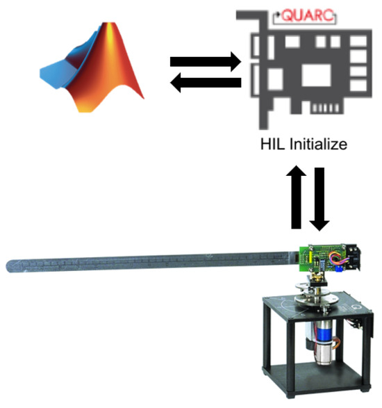
Figure 2. Rotary flexible link communication (Quanser^®).

This is made possible thanks to the virtual laboratory used for this work, as shown in Figure 3. This virtual laboratory provides real data for the acquisition and identification of the system model for the evaluation of different control proposals.

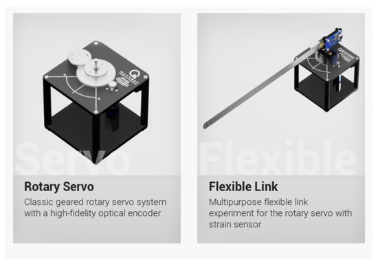
Figure 3. Quanser Interactive Labs (Quanser^®).

The mechanical specifications of the rotary flexible link system are shown in Table 2, according to the information provided by Quanser^®.

Table 2. Physical Parameters [21].

Symbol	Description	Value	Unit
	Module dimensions	48 × 2	${\mathrm{cm}}^2$
$L_1$	Length from strain gauge to end of link	41.9	cm
$m_1$	Flexible link mass	0.065	kg
$I_1$	Flexible link moment of inertia	0.0038	${\mathrm{Kg}·\mathrm{m}}^2$
	Strain gauge bias power	±2	V
	Strain gauge measurement range	±5	V
	Strain gauge calibration gain	1/16.5	Rad/V

For system identification, the following is performed: a square wave voltage is applied to the motor, and the response of the servo motor angle is measured using the rotary encoder, and for the flexible link, the strain gauge. The Simulink model is run using the QUARC Real-Time Control Software, version 2.15 [13] to measure new data or load previously measured data. These data are stored in a file for later use.

t: Time vector related to the motor voltage.

u: Motor voltage values.

$\theta$: Servo angle values.

$\alpha$: Deflection values of the flexible link at the tip.

The state-space model is identified and compared with the measured hardware results without imposing restrictions on the identification shown in Figure 4. The estimated states in the time domain have an estimation of 99.85–96.95% (prediction approach), FPE: $2.89\times {10}^{-13}$, MSE: $1.326\times {10}^{-6}$. As shown, the identified state-space model is quite accurate.

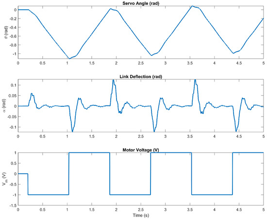
Figure 4. Open − loop response.

Once the model is obtained, it is compared with the actual system data as shown in Figure 5.

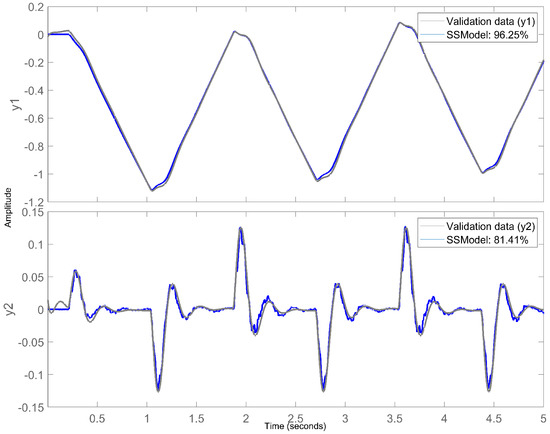
Figure 5. Simulated response comparison.

With the mathematical state-space model obtained, featuring a $96.25\%$ accuracy for $\theta$ and $81.41\%$ accuracy for $\alpha$, the proposed controller is then evaluated.

3. GA-LQR Control

The design of LQR (linear quadratic regulator) control and closed-loop simulation in this context aims to first design a state feedback control based on LQR that is optimal for two main purposes: first, to control the servo position to reach a desired angle and second, to minimize the residual oscillations or vibrations of the flexible link, especially when the servo changes position. To be able to apply the LQR controller, certain criteria must first be checked: identification or verification of the stability of a system by observing the location of the eigenvalues in the complex plane [31].

$$det(sI-A)=s^4+a_1{s}^3+a_2{s}^2+a_{3}s+a_4$$

(74)

The eigenvalues of the system are negative, ensuring its stability. The controllability of the system is also verified; for this, the Kalman controllability criterion is based on the controllable matrix, formed from the matrices $B,AB,A^{2}B,\dots ,A^{n-1}B$, where n is the dimension of the state vector $\mathbf{x}$. If the rank of this matrix equals the dimension of the system’s state space, then it can be asserted that it is completely controllable [32]. In this system, the rank of $\xi$ equals n; therefore, it is completely controllable.

$$\xi =\left[\begin{array}{ccccc}B& AB& A^{2}B& \cdots & A^{n-1}B\end{array}\right]$$

(75)

$$\mathrm{rank}\left(\xi \right)=n$$

(76)

Linear quadratic regulation (LQR) stands out as a powerful technique for controller synthesis. This approach is based on minimizing a quadratic cost function that balances system performance and control effort. By employing LQR, an optimal solution is sought that not only ensures system stability but also optimizes its response according to predefined performance criteria and energy efficiency. The following sections will describe how LQR is utilized to determine the gain matrix K, which is crucial for achieving the desired closed-loop behavior of the system.

LQR control, also known as linear quadratic control, is an optimal control strategy that seeks to maximize the performance of a system through the optimization of a cost function. This technique focuses on solving the regulation problem, which is addressed by minimizing a quadratic index with a linear solution. Thus, LQR control aims to minimize the quadratic function or cost index to improve system performance [33]. It requires the controller to minimize a performance index of the form [34]

$$J={\int }_{t_0}^{\infty }(x^{T}Qx+u^{T}Ru)dt$$

(77)

where Q is a positive definite or positive semidefinite Hermitian matrix of nxn, R is a positive definite Hermitian matrix of rxr, and S is a positive definite or positive semidefinite Hermitian matrix of nxn.

The matrices Q and R determine the relative importance of the error and the cost of this energy.

The control signal is given by:

$$u\left(t\right)=-Kx\left(t\right)$$

(78)

Substituting Equation (78) into Equation (77) gives

$$J={\int }_{t_0}^{\infty }(x^{T}Qx+x^T{K}^{T}RKx)dt$$

(79)

The Hermitian matrix P is real and nxn, and for fully controllable state systems, it is positive definite or positive semidefinite. Equation (80) is equated as follows, and it must comply with the subsequent reduced equation.

$$x^T(Q+K^{T}RK)x=-\left(d\left(x^{T}Px\right)\right)/dt$$

(80)

Deriving the above expression results in

$$x^T(Q+K^{T}RK)x=-{\dot{x}}^{T}Px-x^{T}P\dot{x}=-{\dot{x}}^T[{(A-BK)}^{T}P+P(A-BK)]x$$

(81)

If A – BK is a stable matrix and there exists a positive definite matrix P that satisfies the above equation, then it is satisfied that

$${(A-BK)}^{T}P+P(A-BK)=-(Q+K^{T}RK)$$

(82)

For the determination of R, it is rewritten as $R=T^{T}T$, where T is a nonsingular matrix, having

$${(A-BK)}^{T}P+P(A-BK)+(Q+K^T{T}^{T}TK)=0$$

(83)

Rewriting the previous equation yields

$$A^{T}P+PA+{[TK-T^{-T}BP]}^T[TK-T^{-T}BP]-PB{R}^{-1}{B}^{T}P+Q=0$$

(84)

J is minimized with respect to K from the previous equation, and the following is obtained:

$$K=R^{-1}{B}^{T}P$$

(85)

The matrix K, identified in Equation (85) as the optimal solution, indicates that the most effective control method for tackling the linear quadratic control problem takes on a linear form.

The P matrix from Equation (85) must satisfy the reduced equation, also called the Riccati equation, shown in Equation (86), which has a unique solution. Therefore, it can be concluded that the optimal controller for the linear quadratic regulator problem has a unique solution in the form of a control signal that is a state feedback controller.

$$A^{T}P+PA-PB{R}^{-1}{B}^{T}P+Q=0$$

(86)

Searching for the optimal configuration for matrices Q and R can be complicated. Both manual selection and conventional optimization methodologies often fail to achieve the most effective results, particularly in systems of complex or nonlinear nature [35], where this optimization strategy is applied to determine the optimal values in the LQR matrices used in the control of flexible structures, such as cantilever beams.

Genetic algorithms (GAs), founded on the Darwinian theory of species evolution, seek to find the optimal solution to a problem through the implementation of three distinctive operations that make up their genetics: Selection, crossover, and mutation cycles are repeatedly performed until satisfying a pre-established termination criterion. These algorithms do not require detailed knowledge of the problem to be solved but apply heuristics for the solution, which significantly restricts the number of data needed for their operation [36]. The parameters for the development of the genetic algorithm for this proposal are presented in Table 3.

Table 3. Initial parameters of the proposed GA.

Parameters	Data
Initial population	30
Fitness function	Inverse fitness function
Constraints	Initialization, mutation, post-selection
Selection	Roulette
Crossover	Arithmetic
Crossover probability	90%
Mutation	Uniform
Mutation probability	0.9

The following presents the implementation of a genetic algorithm to optimize the coefficients of the Q and R matrices of the well-known LQR control algorithm according to the requirements for the control design. For this proposal, two parameters of the system dynamics are selected, and the cost function designed for this GA measures these two variables for each system output: overshoot (percentage), the percentage difference between the maximum value and the final value of the controlled signal, and the settling time, which is the time it takes for the signal to remain within 2% of its final value. Finally, it penalizes deviations from these values. The LQR design is based on minimizing the cost function:

$$J={\int }_0^{\infty }\left[x^T\left(t\right)Qx\left(t\right)+u^T\left(t\right)Ru\left(t\right)\right]dt$$

(87)

where:

$x\left(t\right)$ is the state vector.

$u\left(t\right)$ is the control vector.

$Q,R$ are defined weighting matrices.

The cost function design is made to evaluate the performance of a stable, time-invariant, second-order underdamped system with multiple outputs (SIMO: single-input multiple-output). It is based on two important metrics in control system theory: maximum overshoot and settling time. These are crucial metrics in many control applications, as they indicate how quickly and accurately a system can reach and maintain its desired state. It also allows for a quadratic penalty for deviations from desired targets, providing a stronger penalty for larger deviations, which helps guide the algorithm toward solutions that closely match the desired criteria. Furthermore, The cost function balances system performance by penalizing both overshoot and undesirable settling time. Primarily, it is designed with the real characteristics of a control system in mind, so the optimization results will be relevant and applicable in practical scenarios. Lastly, it allows for a clear and quantifiable measure of performance that the algorithm can optimize.

The cost function comprises two main components: the relative maximum oscillation component ($O_S$) and the settling time component ($T_S$).

For the first component, the relative maximum oscillation for each output variable is calculated. This is determined as the maximum change between the values of the variable ($\theta$) and the reference (step signal), expressed as a percentage.

For the second variable ($\alpha$), the oscillation is calculated differently, considering the maximum absolute change relative to the initial value.

If the relative maximum oscillation exceeds a certain threshold, the number of samples before this oscillation occurs is calculated and multiplied by the time interval to obtain the stabilization time ($T_S$) for that variable.

The settling time component ($T_S$) represents the time required for each variable to reach a certain level of stability after undergoing significant oscillations. It is determined as the number of samples before the variable returns within a specific stability threshold and is multiplied by the time interval.

Finally, the cost function aggregates these components for each variable as shown in expression (88).

$$F={(O_{SB}-\gamma )}^2+{(O_{SP}-\gamma )}^2+{(T_{SB}-\beta )}^2+{(T_{SP}-\beta )}^2$$

(88)

where

$O_{SB}$ is the maximum overshoot of the base angle of the RFL.

$O_{SP}$ is the maximum overshoot of the tip angle of the RFL.

$\gamma$ is the desired maximum overshoot.

$T_{SB}$ is the settling time of the base angle of the RFL.

$T_{SP}$ is the settling time of the tip angle of the RFL.

$\beta$ is the desired settling time.

This cost function seeks to penalize solutions that have significant oscillations or take a long time to stabilize. The values of the deviations can change depending on the context of the problem and the designer’s preferences. A lower cost indicates a better and more stable solution in terms of reducing the magnitude of oscillations and the stabilization time of the measured variables.

The $f_n$ function is the cost function, which is described as follows:

Input: matrix y, sampling time $t_s$.

Output: cost function value f, peak overshoot $m{p}_{\mathrm{maxTip}}$, peak overshoot $m{p}_{\mathrm{maxBase}}$, minimum settling time $t_{s_{\min }}$.

• Determine $num\_outputs$ as the number of columns in y.
• Initialize $mp$ (peak overshoots) and $st$ (settling times) arrays to zeros.
• For each output i from 1 to $num\_outputs$:

  (a)

  Extract the i-th column $y_i$ from y.

  (b)

  If i is 2 (special case for the second output):

  -

  Calculate $initial\_value$ as the first element of $y_i$.

  -

  Determine $max\_change$ as the maximum absolute deviation from $initial\_value$.

  -

  Compute the relative peak overshoot $mp\left(i\right)$.

  -

  Update $m{p}_{\mathrm{maxPunt}}$ as the maximum of $max\_change$.

  (c)

  Else (for other outputs):

  -

  Calculate $mp\left(i\right)$ as the relative peak overshoot from the final value.

  -

  Update $m{p}_{\mathrm{maxBase}}$ as the maximum of $mp$.

  (d)

  Determine n as the last time index where the output deviation exceeds 1%.

  (e)

  If no such n is found, set n to 0.

  (f)

  Compute the settling time $st\left(i\right)$ for output i.

• Determine $t{s}_{\min }$ as the minimum settling time across all outputs.
• Compute the cost function f as a weighted sum of squared deviations from desired overshoot and settling time.

The process of interaction of the genetic algorithm with the Simulink model to find the optimal controller parameters is as follows: The initial parameters of the genetic algorithm are established, and the initial population is generated. Each individual in the initial population is evaluated. This involves running the simulation in real-time with each individual’s parameters, followed by calculating the cost function for each set of parameters. The results of this initial evaluation are used to rank the population according to their performance. Then, the GA cycle generates a new temporary population, which includes elite individuals and new individuals created through crossover and mutation. With these results, pairs of individuals are selected, crossover and mutation operations are applied to create new individuals, and restrictions are applied. Finally, for each new individual, a simulation is set up and run using that individual’s parameters, the cost function is calculated for each new parameter configuration, and the population is updated with the new individuals, recalculating the selection probabilities based on the cost function. The parameters of the best individual are used to adjust the controller in the Quanser Interactive Labs virtual scenario.

Below is the control algorithm for the AG-LQR controller:

Definition of constants and parameters:

$$\begin{array}{l}A,B,C,D,t_s=0.01,\\ p_c=0.9,p_m=0.8,\\ N_g=10,N_i=2N_g,\\ N_{\mathrm{gen}}=10N_g,N_e=2,\\ Q_{\min },R_{\min }\end{array}$$

where $A,B,C,D$ are the matrices that define the dynamics of a system in the state equations or transfer functions, $t_s$ is the sampling time in seconds, $p_c$ is the crossover probability in genetic algorithms, indicating the frequency at which pairs of individuals are combined to produce offspring, $p_m$ is the mutation probability in genetic algorithms and reflects the frequency at which individuals undergo random changes, $N_g$ is the population group number, $N_i$ is the population size, $N_{gen}$ is the total number of generations in a genetic algorithm, $N_e$ is the number of elite individuals, and finally $Q_{min}$ and $R_{min}$ are the initialization values for the weighting matrices Q and R in optimal control.

Population initialization:

$$Q_{n_0}=\mathrm{diag}\left([Po{p}_{(n_0,1)}+Po{p}_{(n_0,2)}+\mathrm{zeros}(1,\mathrm{size}(A,1)-2)]\right)$$

(89)

$$R_{n_0}=Po{p}_{(n_0,3)}$$

(90)

Evaluation process of the matrix values Q and R:

$$\mathrm{for}n:i$$

$$Q_n=\mathrm{diag}\left([Po{p}_{(n,1)}+Po{p}_{(n,2)}+\mathrm{zeros}(1,\mathrm{size}(A,1)-2)]\right)$$

(91)

$$R_n=Po{p}_{(n,3)}$$

(92)

$$K=\mathrm{lqr}(\mathrm{sys},Q,R)$$

(93)

$${\mathrm{Sys}}_{\mathrm{cl}}=\mathrm{ss}(A-B\times K,B,C,D,t_s)$$

(94)

$$y_t=\mathrm{step}\left({\mathrm{Sys}}_{\mathrm{cl}}\right)$$

(95)

$$f_n=\cos \mathrm{to}(y_t,t_s)$$

(96)

Fitness function for the GA:

$$F_n=\frac{1}{1+f}$$

(97)

$$P=\frac{F_n}{\sum F_n}$$

(98)

$$P_T=\sum _0^i{P}_i$$

(99)

In this context, $P_T$ is a cumulative probability vector used for the stochastic selection of individuals in the iterative process for the genetic algorithm. Then, the process of selection, crossover, mutation, and insertion is repeated to generate the next generation of the population.

Finally, the K gains are calculated from the optimal values of Q and R obtained that meet the design requirements:

$$q_1=Po{p}_{(1,1)}$$

(100)

$$q_2=Po{p}_{(1,2)}$$

(101)

$$r_1=Po{p}_{(1,3)}$$

(102)

$$Q=\mathrm{diag}\left([q_1,q_2,\mathrm{zeros}(1,\mathrm{size}(A,1)-2)]\right)$$

(103)

$$R=r_1$$

(104)

$$[K_r\sim ]=\mathrm{lqr}(sys,Q,R)$$

(105)

This approach provides a design that allows for the controlling of two parameters of the two output variables, $\theta$ and $\alpha$, demonstrating the computational work of the GA on the dynamic characteristics of the system, the overshoot, and the settling time, which enables one to obtain optimal values for the GA-LQR controller for these two parameters.

4. Lyapunov’s Theorem in GA-LQR Stability Analysis

The stability analysis of the GA-LQR designed controller follows the same fundamental principles of Lyapunov’s stability analysis that apply to any LQR design. The primary difference lies in how the matrices Q and R are selected. The condition $A_{cl}^{T}P+P{A}_{cl}<0$ is a key expression in control theory for verifying the stability of a system using Lyapunov’s Theorem for continuous-time systems.

4.1. Lyapunov’s Theorem

Lyapunov’s theorem is a fundamental tool for determining the stability of dynamic systems without the need to explicitly solve the differential equations describing them. According to this theorem, if a Lyapunov function $V\left(x\right)$ can be found such that:

• $V\left(x\right)>0$ for all $x\ne 0$ (positive definite).
• $\dot{V}\left(x\right)<0$ for all $x\ne 0$ (negative definite time derivative).

Then, the system is stable in the sense of Lyapunov.

4.2. Application to GA-LQR

In the context of LQR, when designing a controller, we transform the system dynamics into a closed-loop form $A_{cl}=A-BK$. To verify the stability of this closed-loop system, we choose $V\left(x\right)=x^{T}Px$ as a candidate Lyapunov function, where P is a symmetric positive definite matrix obtained from solving the Riccati equation.

For the Linear Quadratic Regulator (LQR) method to function correctly and for the solution of the Riccati equation (which produces the matrix P) to ensure stability, the matrices Q and R must satisfy certain properties:

• The matrix Q must be positive semidefinite. This condition ensures that the state variables are properly penalized, contributing to the system’s performance optimization.
• The matrix R must be positive definite. This requirement guarantees that the control effort is penalized, helping to avoid excessive control actions that could destabilize the system.

These properties are crucial for ensuring that the LQR method not only minimizes the quadratic cost function but also maintains the stability of the controlled system [32].

Derivative of $V\left(x\right)$:

The derivative of $V\left(x\right)$ along the trajectories of the system is

$$\dot{V}\left(x\right)={\dot{x}}^{T}Px+x^{T}P\dot{x}$$

Substituting $\dot{x}=A_{cl}x$:

$$\dot{V}\left(x\right)={\left(A_{cl}x\right)}^{T}Px+x^{T}P\left(A_{cl}x\right)$$

$$\dot{V}\left(x\right)=x^T{A}_{cl}^{T}Px+x^{T}P{A}_{cl}x$$

$$\dot{V}\left(x\right)=x^T(A_{cl}^{T}P+P{A}_{cl})x$$

$\dot{x}=A_{cl}x$: This equation demonstrates how the system states x evolve over time under the influence of the controller. The matrix $A_{cl}$ encapsulates both the original dynamics of the system and the influence of the controller. This integrated dynamic model is crucial for understanding and predicting the system’s behavior under controlled conditions.

4.3. Lyapunov Condition

For $\dot{V}\left(x\right)$ to be negative definite, it is necessary that the matrix $A_{cl}^{T}P+P{A}_{cl}$ be negative definite. This is expressed as

$$A_{cl}^{T}P+P{A}_{cl}<0$$

This condition ensures that the Lyapunov function $V\left(x\right)$ decreases along all system trajectories, implying that the closed-loop system is stable.

4.4. Process of Stability Verification

• Matrix Q is positive semidefinite and matrix R is positive definite. While these conditions ensure that the fundamental requirements for the application of the LQR method are met, they alone do not guarantee system stability. It is crucial to perform additional stability verification, as the controller’s ability to stabilize the system depends on the entire closed-loop system dynamics, not just on the positiveness of Q and R. The matrix K derived from the solution to the Riccati equation must be validated to ensure that it leads to a closed-loop system matrix $A_{cl}=A-BK$ with eigenvalues having negative real parts, confirming stability. Simply meeting the positivity conditions of Q and R is necessary but not sufficient; explicit stability checks must be integrated into the control design process to ensure robust and reliable controller performance.
• The system has been analyzed for controllability and the results confirm that the system is fully controllable. The controllability matrix $Co$ is given by:

  $$Co={10}^5\times \left[\begin{array}{cccc}-0.0000& 0.0001& -0.0022& 0.0545\\ 0.0000& -0.0015& 0.0388& -0.5034\\ 0.0001& -0.0035& 0.1596& -5.5443\\ -0.0001& 0.0038& -0.2424& 9.3199\end{array}\right]$$
  The controllability matrix has a rank of 4, indicating that the system is fully controllable. This confirms that any state can be reached from any initial state, ensuring effective response to control inputs across all state variables.
• Obtaining the matrix P through the solution of the Riccati equation:

  $$A^{T}P+PA-PB{R}^{-1}{B}^{T}P+Q=0$$
  The matrix P calculated for our GA-LQR controller is as follows:

  $$P=\left[\begin{array}{cccc}54.7975& -0.1152& 2.3261& 1.0537\\ -0.1152& 5.1686& -4.3326& -2.0855\\ 2.3261& -4.3326& 4.4682& 2.3730\\ 1.0537& -2.0855& 2.3730& 1.3842\end{array}\right]$$
  The symmetry of this matrix ensures the validity of the Lyapunov function used in our stability analysis.
  Furthermore, the eigenvalues of P, which are $\lambda =[0.0405,0.6612,8.6945,13.7583]$, all positive, confirm that P is definitively positive definite, ensuring that our Lyapunov function is adequate for demonstrating the stability of the system.
• Ensuring that the derivative of the Lyapunov function $V\left(x\right)=x^{T}Px$ is negative for all $x\ne 0$. This is a crucial condition indicating that the closed-loop system is stable.
  The closed-loop system matrix $A_{cl}=A-BK$, obtained by applying the feedback control law, is crucial in this analysis. The stability can be verified by examining the eigenvalues of $A_{cl}$. Specifically, the system is stable if all eigenvalues of $A_{cl}$ have negative real parts.
  Using MATLAB, the eigenvalues of the matrix $A_{cl}$ were computed as follows:

  $$\mathrm{Eigenvalues}=\left[\begin{array}{c}-36.6266+0.0000i\\ -9.5173+24.2550i\\ -9.5173-24.2550i\\ -0.1391+0.0000i\end{array}\right]$$
  Analysis of these eigenvalues indicates that all have negative real parts, confirming that the system is stable. This is because the real parts of the eigenvalues, which affect the exponential decay or growth of the system’s response, are all negative.
  The negative real parts of the eigenvalues ensure that $\dot{V}\left(x\right)<0$ for all $x\ne 0$, confirming that the derivative of the Lyapunov function is negative in all cases except the trivial case of $x=0$. This analysis verifies the system’s stability, ensuring that any deviations from the equilibrium state will decay over time, leading to the system settling back to stability.

These steps underline the critical aspects of verifying the stability of a control system designed with optimization techniques, ensuring that despite the modifications in the parameters Q and R, the system remains stable and performs as expected.

5. Evaluation of the GA-LQR Control Results

5.1. Response to a Step Signal

To evaluate the proposed control system, the system’s response is compared to the response generated by an LQR controller.

In (Figure 6), the response of the base position to a step signal is compared due to the LQR control and the GA-LQR control. Both controllers stabilize the system at the desired value. The settling time appears to be fast for both, although it is slightly faster for LQR. The LQR curve shows a rapid rise compared to the GA-LQR curve, indicating a quicker response and possibly better handling of uncertainty or changes in system dynamics.

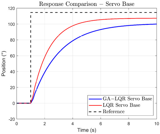
Figure 6. Simulated response comparison.

In (Figure 7), oscillations are due to the nature of the system, here, the GA-LQR response shows a quicker reduction of oscillation, thanks to the control of damping in the system, while the LQR response shows persistent oscillation, indicating a less optimal adjustment to suppress vibrations.

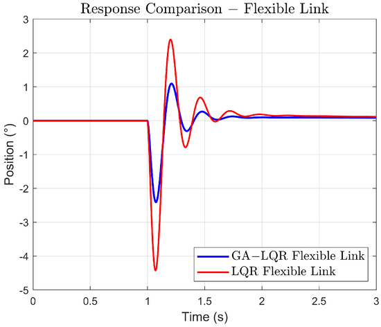
Figure 7. Response comparison of the link tip.

Settling time is hard to determine in oscillatory systems like this, but the goal would be to minimize the amplitude and number of oscillations as shown in Figure 7.

To determine the dynamic characteristics of the system outputs, the discrete model was obtained. Below, Table 4 and Table 5 show the results in response to a step signal.

Table 4. Comparison of the system dynamics (link base) against proposed controllers.

Features	GA-LQR	LQR
Settling Time	7.654	4.854
Overshoot	0	0
Rise Time	4.2680	2.6860
Peak	0.8840	0.9380
Peak Time	15.3980	9.3380
Steady-State Value	0.7964	0.8447

Table 5. Comparison of system dynamics (tip of the link) against proposed controllers.

Characteristic	GA-LQR	LQR
Overshoot	1.1561	2.6557
Peak	0.0216	0.0400
Peak Time	0.0740	0.0700
Steady-State Value	−0.0026	−0.0071

In Figure 7, the oscillations at the tip of the link are observed, comparing the dynamics against the two controllers.

In Table 5, some dynamic characteristics measured at the tip of the link can be observed. It is shown that the design of the proposed algorithm meets the specified requirements, such as significantly reducing oscillations at the tip of the link as outlined in the proposal.

5.2. Error Dynamics in Flexible Link Control Systems

The Figure 8 of the tip error shows that both GA-LQR and conventional LQR experience significant initial error peaks. The GA-LQR reduces the error more quickly and stabilizes with a slightly lower steady-state error compared to the conventional LQR. This suggests that while the GA-LQR is optimized for a quick response, it achieves better steady-state precision at the tip of the link, which is influenced by more complex dynamics due to its flexibility.

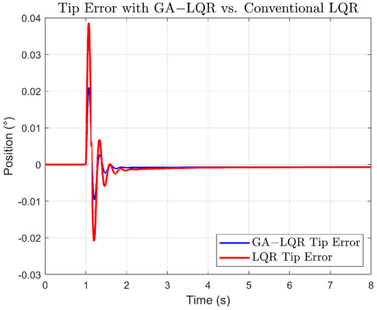
Figure 8. Response comparison of the error Link Tip.

In the Figure 9 of the base error, we observe that both controllers initially also show error peaks. However, the GA-LQR shows a slower reduction of error compared to the conventional LQR and maintains a marginally higher steady-state error. Despite this, the control and correction of the error at the base are more straightforward and effective due to the lower complexity compared with the control of the tip.

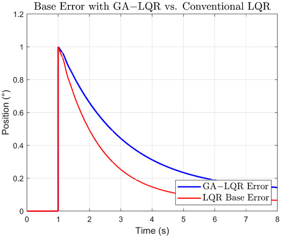
Figure 9. Response comparison of the error base.

Although both controllers are capable of managing errors at the base and the tip, correcting the error at the base is inherently easier due to its more direct control and less complicated dynamics. In contrast, the error at the tip, influenced by the flexibility of the link, requires a more sophisticated approach, making this task more challenging and complex.

5.3. Comparison with Other Controllers

In [37], the control applied to a flexible link system is displayed; it can be compared in Table 6, which shows two measured variables of the dynamics of the tip of the flexible link for four types of controllers: fuzzy, neural network (NN), GA-LQR, and LQR, highlighting differences in their settling times and peak magnitudes. The controllers vary significantly in response speed; the GA-LQR (0.45 s) and LQR (0.7 s) offer fast response times, suitable for applications that demand quick corrections, whereas the fuzzy controller, with a settling time of over 60 s, is much slower, being suitable for applications where precision is more important than speed, and the NN (9 s) provides a balance between rapid response and moderate control. Regarding the magnitude of the peaks, the GA-LQR shows the smallest peak (0.0216), indicating smooth control and minimal disturbance, ideal for sensitive systems. On the other hand, the LQR, although effective, generates higher oscillations (0.0400), and both fuzzy and NN maintain moderate peaks (0.0573), suggesting proper management of oscillations without inducing major disturbances.

Table 6. Comparison of system dynamics for additional controllers.

Features	Fuzzy	NN	GA-LQR	LQR
Settling time (s)	>60	9	0.45	0.7
Peak (º)	0.0573	0.0573	0.0216	0.0400

5.4. Constant Periodic Amplitude Trajectory

The evaluation of controllers with a constant periodic signal is crucial for determining the system’s ability to accurately and stably follow repetitive trajectories. This simulation reveals the system’s response to cyclic inputs, essential in applications such as engines and robots where precision in recurrent movements is required.

As observed in Figure 10 and Figure 11, against a constant periodic amplitude trajectory, the GA-LQR controller is a better option compared to an LQR controller for a flexible rotary system where vibration suppression and smooth transition are critical. It is noted that the energy transmission from the base to the tip of the flexible link is more controlled under GA-LQR control, causing a lower amplitude of tip oscillations, as seen in Figure 11, while the LQR control, due to its more aggressive response at the base, transmits less controlled energy along the link, resulting in a more vibrant response.

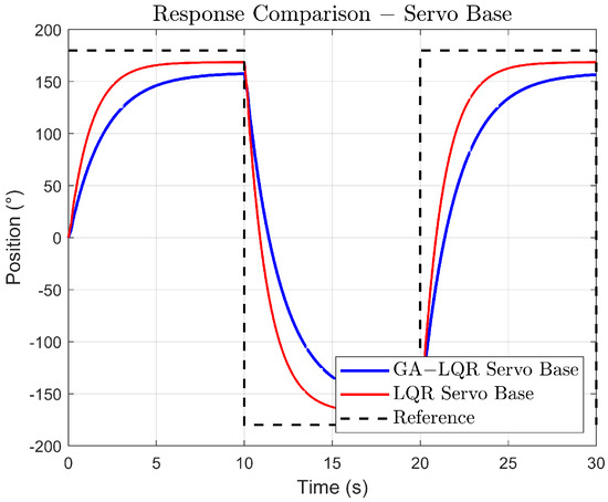
Figure 10. Response comparison for constant periodic amplitude trajectory of the link base.

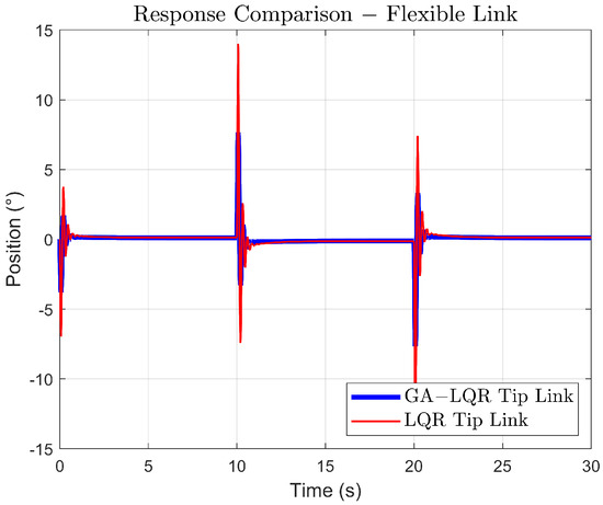
Figure 11. Response Comparison for constant periodic amplitude trajectory of the link tip.

5.5. Increasing Amplitude Trajectory

Trials conducted in engineering contexts, such as in crane robots and flexible manipulators, indicate that different controllers play a crucial role in reducing vibrations during repetitive movements that feature variable setpoint profiles [38]. Figure 12 and Figure 13 highlight that, for an increasing amplitude trajectory, the control scheme offers similar performance in vibration suppression, keeping the maximum deflection angle restricted. Although there is an initial deviation in tracking during the transient phase, it offers smooth tracking in certain cases, like in the square trajectory.

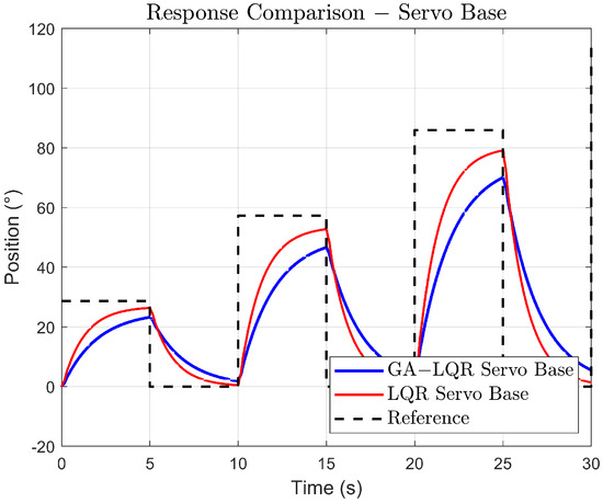
Figure 12. Comparison of the link base response to increasing gain.

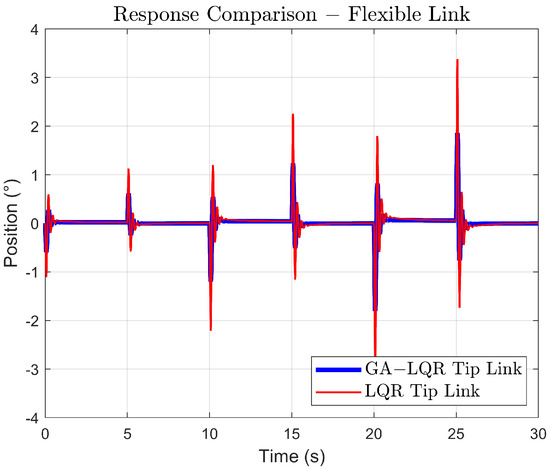
Figure 13. Comparison of the link tip response to increasing gain.

In Figure 12, for the base of the system, the GA-LQR controller reaches and follows the reference with less precision and shows a slower response than the standard LQR. In Figure 13, the GA-LQR demonstrates a reduction in the amplitude of oscillations compared to the LQR, showing a better capability of controlling vibrations induced by the flexibility of the link. This is crucial in systems where vibration control is fundamental for the precision and structural integrity of the system.

In Figure 14, one of the transitions in response to an increasing amplitude trajectory has been amplified, and it is observed that the LQR response shows greater amplitude in oscillations, indicating a less damped response and a more aggressive control approach. In contrast, the GA-LQR appears to dampen oscillations more quickly, which is desirable in applications where precision and stability are required. Similarly, the time it takes each controller to stabilize the response after a transition is observed. The GA-LQR shows faster stabilization, suggesting a better adaptation to the dynamic conditions of the system.

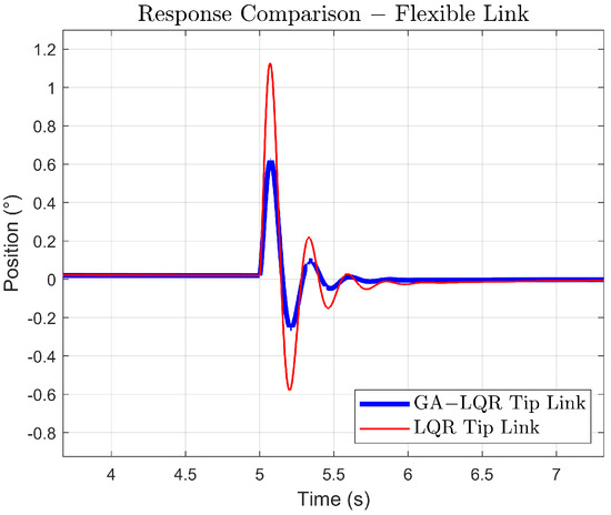
Figure 14. Comparison of the link tip’s response to a transition with increasing gain.

Overall, the results indicate that the GA-LQR offers a significant improvement in the control of flexible rotary systems, effectively balancing tracking speed and vibration attenuation.

5.6. Performance Comparison of GA-LQR and LQR Control Systems

The transmissibility metrics are vital in this analysis, highlighting the effectiveness of controllers in damping vibrations.

To understand how a structure responds to vibration introduced at its base, in [39], a mass on a spring is considered, which is referred to as a single-degree-of-freedom (SDOF) system, with a unitary sinusoidal acceleration (1 g) introduced at the base of the spring. The transmissibility function, $TR\left(f_{\mathrm{ratio}}\right)$, provides the peak response. The acceleration of the mass as a function of $f_{\mathrm{ratio}}$, which is the ratio of the input frequency f to the natural frequency $f_n$ of the SDOF system, is expressed next.

The transmissibility function, $T_R\left(f_{\mathrm{ratio}}\right)$, is defined as

$$T_R\left(f_{\mathrm{ratio}}\right)=\sqrt{\frac{1+{\left(2\zeta f_{\mathrm{ratio}}\right)}^2}{{(1-f_{\mathrm{ratio}}^2)}^2+{\left(2\zeta f_{\mathrm{ratio}}\right)}^2}}$$

where $\zeta$ is the damping ratio (damping factor divided by the critical damping factor). It shows the transmissibility function for various damping ratios, indicating how the vibrational energy from the base or motor affects the tip of the link, we consider the following:

Low Frequency Robustness: Crucial since rotary systems tend to exhibit low-frequency oscillations due to imbalances.

High-Frequency Noise Sensitivity: Important, as less energetic high-frequency vibrations should not be amplified to maintain precision.

Peak Response: Critical in a flexible link, excessive peaks could cause displacements exceeding design limits or induce material fatigue.

Transmissibility indicates how much vibrational energy from the base or motor affects the tip of the link. The data suggest that the GA-LQR, with its lower peak response, might better control these vibrations. Both the GA-LQR and LQR systems demonstrate transmission ratios close to unity across most frequency ranges, indicating that the output is approximately equal to the input in terms of amplitude. However, the LQR system features a pronounced peak near 10 rad/s, suggesting heightened sensitivity at this resonance frequency. This could potentially amplify any disturbances or inputs at this specific frequency. In contrast, the GA-LQR system also exhibits a peak, albeit less pronounced, which suggests better suppression of resonance compared to the LQR system.

The peak of the GA-LQR is narrower compared to that of the LQR, indicating that the GA-LQR system is more selective in terms of frequency. This might be desirable if only a specific frequency needs to be amplified or attenuated. At high frequencies, both systems show good attenuation, which is desirable to minimize the impact of noise and other unwanted signals typically present at these frequencies. The LQR appears to offer a smoother response and is less prone to pronounced resonances, which might be more suitable in applications where large amplifications due to certain input frequencies are undesirable. On the other hand, the GA-LQR might be more appropriate in applications where greater sensitivity or control at a specific frequency is needed.

The Table 7 compares the GA-LQR and LQR control systems, highlighting their performance in low-frequency robustness, high-frequency noise sensitivity, and resonance peak overshoot. The GA-LQR outperforms the LQR in reducing noise sensitivity and managing resonances, offering a more stable response. Although the LQR is more susceptible to noise, its robustness makes it suitable for less demanding applications, emphasizing the need to select the appropriate controller based on design specifications.

Table 7. Comparative analysis of GA-LQR and LQR control systems.

Metric	GA-LQR	LQR
Low-Frequency Robustness	1.000108	1.000114
High-Frequency Noise Sensitivity	1.000102	1.000257
Resonance Peak Overshoot	0.006821	0.014163

6. Conclusions

This study has effectively demonstrated how the modeling and control of a single-degree-of-freedom flexible robotic link can be efficiently managed using the Euler–Lagrange method and LQR controller. The integration of a genetic algorithm for optimizing the Q and R matrices has proven to be an innovative solution that successfully addresses the complexity of their configuration. Looking forward, plans are in place to apply and expand this method to more complex and multilink robotic system configurations, leveraging the robustness and flexibility of the GA to tackle greater challenges and complexities in the field of robotics.

This article has presented an GA-LQR controller to address the problem of tracking and vibration suppression of the flexible manipulator. By using GA to optimize Q and R, this allows us to explore a larger solution space and potentially find parameter combinations that would not be obvious or easy to test manually. In the GA-LQR control, classic control design criteria such as percentage overshoot, settling time, etc., are directly incorporated into the algorithm’s cost function, allowing one to align Q and R parameters with the specific design objectives of the controller. The GA-LQR control algorithm is versatile for multivariable systems, optimizing design variables via specialized cost functions to meet specific requirements. However, the selection of priorities within the system settings depends on the control engineer. This decision shapes the algorithm’s effectiveness in achieving control objectives, underscoring the engineer’s crucial role in customizing the implementation to the system’s needs.

The results in the simulations clearly confirm that the proposed control system minimizes the end vibrations of the manipulator as requested in the design of the genetic algorithm. This research has provided a general methodology for enforcing certain design requirements for position control of the tip of a rotating flexible link using genetic algorithm techniques over an LQR for the optimization of desired parameters.

Using a reference model for the GA allows us to ensure that the resulting parameters are aligned with a known desired behavior. However, the reference model must be representative enough of the real system for the optimized parameters to be effective in practice.

For future work, the challenge of using the GA-LQR control in real time is proposed. One approach could consider the possibility of running the GA on a slower cycle, where upon finding variations from the expected model, it reviews and adjusts the LQR parameters based on the system’s recent performance, while a faster LQR controller handles real-time control. Lastly, an improvement would be to develop a faster and more efficient version of the GA that can run in real time or near-real time.

References

- Ding, B.; Li, X.; Chen, S.C.; Li, Y. Modular quasi-zero-stiffness isolator based on compliant constant-force mechanisms for low-frequency vibration isolation. J. Vib. Control. 2023, 10775463231188160. [Google Scholar] [CrossRef]
- Boscariol, P.; Scalera, L.; Gasparetto, A. Nonlinear Control of Multibody Flexible Mechanisms: A Model-Free Approach. Appl. Sci. 2021, 11, 1082. [Google Scholar] [CrossRef]
- Hernández, M.L.A.; de León Morales, J. Design of Different Controllers for a Flexible Robot in the Link. Ph.D. Thesis, Technological Institute of Nuevo Laredo, San Nicolás de los Garza, Mexico, 2024. Available online: http://eprints.uanl.mx/5760/1/1020126752.PDF (accessed on 10 May 2024).
- Sorcia-Vázquez, F. Control of a Flexible Link Robot Arm through Generalized PID and Model-Free Control. 2010. Available online: https://example.com/flexible-link-control (accessed on 15 October 2023).
- Ding, B.; Li, X.; Li, C.; Li, Y.; Chen, S.C. A survey on the mechanical design for piezo-actuated compliant micro-positioning stages. Rev. Sci. Instruments 2023, 94, 101502. [Google Scholar] [CrossRef]
- Aktas, K.G.; Esen, I. State-Space Modeling and Active Vibration Control of Smart Flexible Cantilever Beam with the Use of Finite Element Method. Eng. Technol. Appl. Sci. Res. 2020, 10, 6549–6556. [Google Scholar] [CrossRef]
- Jafari, M. Linear Quadratic Regulator with Genetic Algorithm for Flexible Structures Vibration Control. Master’s Thesis, Universiti Putra Malaysia, Seri Kembangan, Malaysia, 2015. [Google Scholar]
- Schoen, M.P.; Hoover, R.C.; Chinvorarat, S.; Schoen, G.M. System Identification and Robust Controller Design Using Genetic Algorithms for Flexible Space Structures. J. Dyn. Syst. Meas. Control 2009, 131, 031003. [Google Scholar] [CrossRef]
- Liu, M.; Cao, D.; Li, J.; Zhang, X.; Wei, J. Dynamic Modeling and Vibration Control of a Large Flexible Space Truss. Meccanica 2022, 57, 1017–1033. [Google Scholar] [CrossRef]
- Becerra, J.E.T. Fractional Order Modeling of Contact with the Environment in Flexible Robot Applications. 2018. Available online: https://ruc.udc.es/dspace/handle/2183/24982 (accessed on 6 December 2023).
- Quanser. Quanser Interactive Labs for Distance & Blended Control Systems and Robotics Courses. Available online: https://www.quanser.com/event-webinar/quanser-interactive-labs-for-distance-blended-control-systems-and-robotics-courses/ (accessed on 12 January 2024).
- Anayi, F.; Packianather, M.; Samad, B.A.; Yahya, K. Simulating LQR and PID controllers to stabilise a three-link robotic system. In Proceedings of the 2022 2nd International Conference on Advance Computing and Innovative Technologies in Engineering (ICACITE), Greater Noida, India, 28–29 April 2022; pp. 2033–2036. [Google Scholar] [CrossRef]
- Quanser. QLabs Virtual Rotary Flexible Link-Credible Lab Activities Off-Campus. 2022. Available online: https://www.quanser.com/products/qlabs-virtual-rotary-flexible-link/ (accessed on 16 August 2023).
- Mohamed, Z.; Martins, J.; Tokhi, M.; Costa, J.D.; Botto, M. Vibration Control of a Very Flexible Manipulator System. Control Eng. Pract. 2005, 13, 267–277. [Google Scholar] [CrossRef]
- He, X.; Zhang, S.; Ouyang, Y.; Fu, Q. Vibration Control for a Flexible Single-Link Manipulator and Its Application. IET Control Theory Appl. 2020, 14, 930–938. [Google Scholar] [CrossRef]
- Rao, J. Advanced Theory of Vibration; Wiley: New York, NY, USA, 1991. [Google Scholar]
- Meirovitch, L. Methods of Analytical Dynamics; Dover Publications: Garden City, NY, USA, 1970. [Google Scholar]
- Tokhi, M.; Azad, A. Flexible Robot Manipulators: Modelling, Simulation and Control; IET: London, UK, 2008; Volume 68. [Google Scholar]
- Tse, F.; Morse, I.; Hinkel, R. Mechanical Vibrations: Theory and Applications; Allyn & Bacon Inc.: Boston, MA, USA, 1978. [Google Scholar]
- Cannon, R.; Schmitz, E. Initial Experiments on the End-Point Control of a Flexible One-Link Robot. Int. J. Robot. Res. 1984, 3, 62–75. [Google Scholar] [CrossRef]
- Tokhi, M.; Azad, A. Flexible Robot Manipulators: Modelling, Simulation and Control; The Institution of Engineering and Technology: London, UK, 2017. [Google Scholar]
- Subedi, D.; Tyapin, I.; Hovland, G. Review on Modeling and Control of Flexible Link Manipulators. Model. Identif. Control 2020, 41, 141–163. [Google Scholar] [CrossRef]
- Pham, P.T.; Kim, G.H.; Nguyen, Q.; Hong, K.S. Control of a Non-uniform Flexible Beam: Identification of First Two Modes. Int. J. Control Autom. Syst. 2021, 19, 3698–3707. [Google Scholar] [CrossRef]
- Hughes, P. Space structure vibration modes: How many exists? Which ones are important? IEEE Control Syst. Mag. 1987, 7, 22–28. [Google Scholar] [CrossRef]
- University of New York. Modeling of a Flexible Link. 2024. Available online: http://engineering.nyu.edu/mechatronics/Mpcrl/WebExp/Flexiblelink/Modeling/index.html.htm (accessed on 28 April 2024).
- Sorcia-Vázquez, F.J.; García-Beltrán, C.D.; Reyes-Reyes, J.; Rodríguez-Palacios, A. Control of a Flexible Link Robot Arm Using Generalized PID and Model-Free Control; National Center for Research and Technological Development: Cuernavaca, Morelos, Mexico; Technological Institute of Zacatepec: Zacatepec, Morelos, Mexico, 2023. [Google Scholar]
- Ahmad, M.; Mohamed, Z.; Hambali, N. Dynamic Modelling of a Two-Link Flexible Manipulator System Incorporating Payload. In Proceedings of the 2008 3rd IEEE Conference on Industrial Electronics and Applications, Singapore, 3–5 June 2008; pp. 96–101. [Google Scholar] [CrossRef]
- Khairudin, M. Dynamic Modelling of a Flexible Link Manipulator Robot Using AMM. TELKOMNIKA 2008, 6, 6. [Google Scholar] [CrossRef][Green Version]
- Restrepo, D. The Lagrangian of the Standard Model; Institute of Physics, University of Antioquia: Medellín, Colombia, 2012. [Google Scholar]
- Arenas, T.C. Dynamic Analysis of a Flexible Mechanism by Finite Elements. Ph.D. Thesis, Universidad Nacional Autónoma de México, Faculty of Engineering, Ciudad Universitaria, Mexico City, Mexico, 2016. [Google Scholar]
- Abreu, V.V. Balance-Bot-ProQuest. 2009. Available online: https://www.proquest.com/openview/080d5273c83b3058e802b3684705a356/1?pq-origsite=gscholar&cbl=2026366&diss=y (accessed on 15 January 2024).
- Braschi, E.A. Practical Approach to Modern Control. Published by Casa del Libro. 2024. Available online: https://www.casadellibro.com/libro-practical-approach-to-modern-control/9786124191282/7580541 (accessed on 12 January 2024).
- Peñafiel, D.K.S. Design and Implementation of an Optimal LQG Controller for an Inverted Pendulum System Applied to LEGO Mindstorms Equipment. Ph.D. Thesis, Salesian Polytechnic University, Quito Campus, Quito, Ecuador, 2018. [Google Scholar]
- Ogata, K. Discrete-Time Control Systems. Available online: http://www2.pelotas.ifsul.edu.br/~coutinho/disciplinas/TCC/Discrete-Time_Control_Systems-Katsuhiko_Ogata.pdf (accessed on 15 January 2024).
- Lorbes, M. Genetic Algorithms and Particle Switching Optimization to Define the Weight Matrices of the Linear Quadratic Regulator Methodology. Univ. Sci. Technol. 2020, 24, 34–41. [Google Scholar]
- Raoufi, M.; Delavari, H. Designing a Model-Free Reinforcement Learning Controller for a Flexible-Link Manipulator. In Proceedings of the 2021 9th RSI International Conference on Robotics and Mechatronics (ICRoM), Tehran, Iran, 17–19 November 2021; pp. 1–6. [Google Scholar] [CrossRef]
- López, J.C. Control of a Single-Segment Flexible Manipulator. 2022. Available online: http://hdl.handle.net/10902/24745 (accessed on 15 May 2022).
- Viswanadhapalli, J.; Elumalai, V.; Shivram, S.; Shah, S.; Mahajan, D. Deep Reinforcement Learning with Reward Shaping for Tracking Control and Vibration Suppression of Flexible Link Manipulator. Appl. Soft Comput. 2023, 152, 110756. [Google Scholar] [CrossRef]
- Sarafin, T.; Doukas, P.; Demchak, L.; Browning, M. Introduction to Vibration Testing. Instar Engineering and Consulting, Inc., Rev. B. 2017. Available online: https://s3vi.ndc.nasa.gov/ (accessed on 16 December 2023).
Disclaimer/Publisher’s Note: The statements, opinions and data contained in all publications are solely those of the individual author(s) and contributor(s) and not of MDPI and/or the editor(s). MDPI and/or the editor(s) disclaim responsibility for any injury to people or property resulting from any ideas, methods, instructions or products referred to in the content. |
© 2024 by the authors. Licensee MDPI, Basel, Switzerland. This article is an open access article distributed under the terms and conditions of the Creative Commons Attribution (CC BY) license (https://creativecommons.org/licenses/by/4.0/).