Cyanide Molecular Laser-Induced Breakdown Spectroscopy with Current Databases

Abstract

This work discusses diatomic molecular spectroscopy of laser-induced plasma and analysis of data records, specifically signatures of cyanide, CN. Line strength data from various databases are compared for simulation of the CN, $B{}^2{\Sigma }^{+}⟶X{}^2{\Sigma }^{+}$, $\Delta \mathrm{v}=0$ sequence. Of interest are recent predictions using an astrophysical database, i.e., ExoMol, a laser-induced fluorescence database, i.e., LIFBASE, and a program for simulating rotational, vibrational, and electronic spectra, i.e., PGOPHER. Cyanide spectra that are predicted from these databases are compared with line-strength data that have been in use by the author for the last three decades in the analysis of laser–plasma emission spectra. Comparisons with experimental laser–plasma records are communicated as well for spectral resolutions of 33 and 110 picometer. The accuracy of the CN line-strength data is better than one picometer. Laboratory experiments utilize 308 nm, 35 picosecond bursts within an overall 1 nanosecond pulse-width, and 1064 nm, 6 ns pulse-width radiation. Experimental results are compared with predictions. Differences of the databases are elaborated for equilibrium of rotational and vibrational modes and at an internal, molecular temperature of the order of 8,000 Kelvin. Applications of accurate CN data include, for example, combustion diagnosis, chemistry, and supersonic and hypersonic expansion diagnosis. The cyanide molecule is also of interest in the study of astrophysical phenomena.

1. Introduction

The diatomic molecule cyanide, CN, occurs in various forms in nature. The toxicity of cyanide motivates health studies, in particular those of hydrogen cyanide gas that kills by inhalation. Cyanide radical measurements characterize interstellar clouds, including temperature inferences of the cosmic microwave background radiation [1,2]. The primary interest in this work is the CN violet $B{}^2{\Sigma }^{+}-X{}^2{\Sigma }^{+}$ band systems. Extensive experimental and theoretical details convey the complexity of the CN radical [3,4]. In particular, the CN red systems are mentioned in a study of laboratory spectroscopy of astrophysically interesting molecules [5].

Spectroscopy [6,7,8,9,10] of laser-induced air plasma reveals “fingerprints” of CN early (within the first microsecond) in the plasma decay [11]. Recent developments of laser-induced breakdown spectroscopy indicate interest in the diagnosis of molecular species. This work investigates existing databases for diatomic molecules, in particular the ones for CN, for analysis of measured emission spectra. Laser-induced breakdown with 6 ns, 1064 nm radiation and associated diagnosis [12] discusses the determination of CN distribution and shock-wave phenomena in hypersonic and supersonic expansion.

For cyanide spectroscopy, one can employ the ExoMol database [13], the LIFBASE laser-induced fluorescence database [14], and the PGOPHER program for simulating rotational, vibrational, and electronic spectra [15]. There are, of course, other databases that can be accessed [16] for diatomic molecules, including HITEMP that, for example, shows hydroxyl, OH, data [17]. The ExoMol, LIFBASE, and PGOPHER predictions of the CN violet $\Delta \mathrm{v}=0$ sequence are compared with experimental data. The laser–plasma recombination spectra that are utilized in the comparisons were captured following optical breakdown with picosecond laser pulses in a 1:1 molar CO${}_2$:N${}_2$ atmospheric gas mixture and in standard ambient temperature and pressure laboratory conditions. Astrophysical ExoMol databases are expected to work well for optical spectroscopy of laser–plasma. The measurement of molecular spectra may be accomplished with nanosecond laser-induced optical breakdown—molecular spectra are readily observed with femtosecond or picosecond laser–plasma excitation—after some time delay (of the order larger than 100 ns for the occurrence of CN in CO${}_2$:N${}_2$ gas mixtures) from optical breakdown when using nanosecond laser pulses. In addition, analysis is discussed with previously established line-strength data that are freely available along with MATLAB [18] scripts for a subset of transitions associated with the CN violet and red band systems [19,20].

2. Materials and Methods

Computation of optical molecular spectra relies on sets of wavelength positions and line strengths for molecular band systems with, in principle, theoretically resolved vibrational and rotational transitions. Experimental spectral resolutions discussed in this work are 0.033 nm to 0.11 nm. Consequently, there are a multitude of lines for each wavelength-bin of a digital array detector that captures time-resolved data following individual laser–plasma events. For example, there are well over 2000 lines in the CN violet $\Delta \mathrm{v}=0$ spectral region of 370 nm to 390 nm, and most lines are bunched together, including overlapped vibrational band heads. The measurements utilize a typical laser-induced optical breakdown experimental arrangement [21], namely, (i) laser device, (ii) focusing lens, (iii) cell that contains the atmospheric mixture, (iv) spectrometer, (v) linear diode detector and optical multichannel analyzer, (vi) electronic timing, and (vii) monitor devices and equipment for subsidiary measurements capturing time-resolved CN B-X data

2.1. Traditional Simulation of Diatomic Molecular Spectra

The traditional approach for the generation of simulated spectra is based on molecular constants. The energy levels can be evaluated by employing a Dunham expansion [22],

$$E(\mathrm{v},J)=\sum _{k,l}{Y}_{k,l}{(\mathrm{v}+1/2)}^k{\left[J(J+1)\right]}^l.$$

(1)

The constant coefficients $Y_{k,l}$ are called Dunham parameters, with the indices k and l corresponding to vibrational and rotational contributions, respectively. The $k=0$ and $l=0$ parameter $Y_{0,0}$ represents the minimum electronic energy, $T_e$.

Table 1. Spectroscopic constants for the A–X and B–X transitions of ${}^{12}{\mathrm{C}}^{14}\mathrm{N}$.

${\mathit{Y}}_{\mathit{k},\mathit{l}}$	Constant	X${}^2{\mathit{\Sigma }}^{+}$ (${\mathbf{cm}}^{-1}$)	A${}^2\mathit{\Pi }$ (${\mathbf{cm}}^{-1}$)	B${}^2{\mathit{\Sigma }}^{+}$ (${\mathbf{cm}}^{-1}$)
$Y_{0,0}$	$T_e$	0.0	9245.28	25,752.0
$Y_{1,0}$	${\omega }_e$	2068.59	1812.5	2163.9
$-Y_{2,0}$	${\omega }_e{x}_e$	13.087	12.60	20.2
$Y_{3,0}$	${\omega }_e{y}_e$	$-0.00909$	−0.0118	–
$Y_{0,1}$	$B_e$	1.8997	1.7151	1.973
$-Y_{1,1}$	${\alpha }_e$	0.01736	0.01708	0.023
$Y_{2,1}$	${\gamma }_e$	$-3.10\times {10}^{-5}$	$-3.6\times {10}^{-5}$	–
$-Y_{0,2}$	$D_e$	$6.40\times {10}^{-6}$	$5.93\times {10}^{-6}$	$\left[6.6\times {10}^{-6}\right]$
$-Y_{1,2}$	${\beta }_e$	$12\times {10}^{-9}$	$42\times {10}^{-9}$	–

lists the molecular constants in units of ${\mathrm{cm}}^{-1}$ for the A–X and B–X transitions for ${}^{12}{\mathrm{C}}^{14}\mathrm{N}$ [23].

The application of traditional molecular constants (see Table 1) is expected to reveal line-position and intensity inconsistencies. For example, air emission spectra predictions with the NEQAIR code [24,25] reveal slightly different line positions leading to difficulties in air–plasma analysis of superposition spectra composed of several species. The laser plasma that is generated in dry air shows a variety of species [26,27,28]; consequently, accurate predictions of individual components are desirable. Commercial SPECAIR software is available that focuses on calculating emission or absorption spectra of air plasma radiation [29]. Conversely, one can utilize published molecular line positions and strengths for individual species for the spectra simulation of the CN diatomic molecule, as further elaborated in Section 2.2, Section 2.3 and Section 2.4.

2.2. Line Positions and Strengths of Diatomic Spectra

In this work, the computation of diatomic molecular spectra utilizes line-strength data. The Boltzmann equilibrium spectral program (BESP) and the Nelder–Mead temperature (NMT) program allow one to respectively compute an emission spectrum and fit theoretical to experimental spectra. The construction of the communicated molecular CN line strengths “CNv-lsf” [20] first makes use of Wigner–Witmer eigenfunctions and a diatomic line position fitting program. Second, it computes Frank–Condon factors and r-centroids, and third, it combines these factors with the rotational factors that usually decouple from the overall molecular line strength due to the symmetry of diatomic molecules. In turn, the ExoMol states and transition files for CN [4,30,31] and the PGOPHER data file [32] are examined in order to generate line-strength data that can be used with BESP and NMT. The LIFBASE program is utilized for visual comparisons of CN B-X simulated and recorded data.

The ExoMol and the PGOPHER data show Einstein A-coefficients that are converted to line strengths [33,34,35], S, for electric dipole transitions, using

$$A_{ul}=\frac{16{\pi }^3}{3g_{u}h{\mathsf{ϵ}}_0{\mathsf{\lambda }}^3}{\left(e{a}_0\right)}^2{S}_{ul},g_u=2(2J_u+1).$$

(2)

Here, $A_{ul}$ denotes the Einstein A-coefficient for a transition from an upper, u, to a lower, l, state, and h and ${\epsilon }_0$ are Planck’s constant and vacuum permittivity, respectively. The elementary charge is e, the Bohr radius is $a_0$, and the transition strength is $S_{ul}$. The line strength, S, that is used in the MATLAB scripts is expressed in traditional spectroscopy units (stC${}^2$ cm${}^2$). The wavelength of the transition is $\mathsf{\lambda }$, $g_u$ is the upper state degeneracy, and $J_u$ is the total angular momentum of the upper state.

2.3. Wigner–Witmer Diatomic Eigenfunction

The Hund’s case (a) basis functions (explicitly, see Equation (6) below) are derived from the Wigner and Witmer [36,37] diatomic eigenfunction,

$$\langle \rho ,\zeta ,\chi ,{\mathbf{r}}_2,\cdots ,{\mathbf{r}}_N,r,\theta ,\varphi |n\mathrm{v}JM\rangle =\sum _{\Omega =-J}^J\langle \rho ,\zeta ,{\mathbf{r}}_2^{\prime },\cdots ,{\mathbf{r}}_N^{\prime },r|n\mathrm{v}\rangle D_{M\Omega }^{J^{*}}(\varphi ,\theta ,\chi ).$$

(3)

The coordinates include the distance, $\rho$, of one electron (the electron arbitrarily labeled 1, but it could be any one of the electrons) from the internuclear vector, $\mathbf{r}(r,\theta ,\varphi )$, the distance, $\zeta$, of that electron above or below the plane perpendicular to $\mathbf{r}$ and passing through the center of mass of the two nuclei (the coordinate origin), the angle, $\chi$, for rotation of that electron about the internuclear vector $\mathbf{r}$, and the remaining electronic coordinates ${\mathbf{r}}_2,\cdots ,{\mathbf{r}}_N$ in the fixed and ${\mathbf{r}}_2^{\prime },\cdots ,{\mathbf{r}}_N^{\prime }$ in the rotating coordinate system. The vibrational quantum number $\mathrm{v}$ has been extracted from the quantum number collection n that represents all required quantum numbers except J, M, $\Omega$, and $\mathrm{v}$. The Wigner–Witmer diatomic eigenfunction is well-suited for the description of the diatomic molecule. The exact separation of the Euler angles represents a clear advantage over the Born–Oppenheimer approximation for the diatomic molecule in which the angle of electronic rotation, $\chi$, is unnecessarily separated from the angles describing nuclear rotation, $\theta$ and $\varphi$. Equation (3) can be derived by writing the general equation for coordinate (passive) rotations $\alpha$, $\beta$, and $\gamma$ of the eigenfunction, replacing two generic coordinate vectors with the diatomic vectors $\mathbf{r}(r,\theta ,\varphi )$ and ${\mathbf{r}}^{\prime }(\rho ,\zeta ,\chi )$, and equating the angles of coordinate rotation to the angles of physical rotation $\varphi$, $\theta$, and $\varphi$. The general equation for coordinate rotation holds in isotropic space, and therefore, the quantum numbers J, M, and $\Omega$, in the Wigner–Witmer eigenfunction include all electronic and nuclear spins.

The rotation matrix element $D_{M\Omega }^J(\varphi ,\theta ,\chi )$ and its complex conjugate $D_{M\Omega }^{J^{*}}(\varphi ,\theta ,\chi )$ do not fully possess the mathematical properties of quantum mechanical angular momentum. It is well-known that a sum of Wigner D-functions is required to build an angular momentum state. The equation

$$J_{\pm }^{\prime }{D}_{M\Omega }^{J^{*}}(\varphi ,\theta ,\chi )=\sqrt{J(J+1)-\Omega (\Omega \mp 1)}{D}_{M,\Omega \mp 1}^{J^{*}}(\varphi ,\theta ,\chi )$$

(4)

is a mathematical result readily obtained from Equation (3) and

$$J_{\pm }^{\prime }|J\Omega \rangle =\sqrt{J(J+1)-\Omega (\Omega \pm 1)}|J,\Omega \pm 1\rangle ,$$

(5)

in which the prime on the operator $J_{\pm }^{\prime }$ indicates that it is written in the rotated coordinate system where the appropriate magnetic quantum number is $\Omega$.

The Hund’s case (a) basis function based upon the Wigner–Witmer diatomic eigenfunction, with the spin ket $|S\Sigma \rangle$, equals

$$\begin{array}{ccc}\hfill |a\rangle & =& \hfill \langle \rho ,\zeta ,\chi ,{\mathbf{r}}_2^{\prime },\cdots ,{\mathbf{r}}_{\mathcal{N}}^{\prime },r,\theta ,\varphi |n\mathrm{v}JM\Omega L\Lambda S\Sigma \rangle \hfill \\ & =& \hfill \sqrt{\frac{2J+1}{8{\pi }^2}}\langle \rho ,\zeta ,{\mathbf{r}}_2^{\prime },\cdots ,{\mathbf{r}}_{\mathcal{N}}^{\prime },r|n\mathrm{v}\rangle |S\Sigma \rangle D_{M\Omega }^{J^{*}}(\varphi ,\theta ,\chi ).\hfill \end{array}$$

(6)

As noted above, a sum of $|a\rangle$ basis functions is required to build an eigenstate of angular momentum.

The prediction of diatomic spectra and establishment of the CNv-lsf database involves (a) determination of accurate wavenumbers for the transition and rotational line strengths, viz. Hönl–London values (see details below in Section 2.4), (b) vibrational transition strengths, viz. Frank–Condon factors from eigenfunctions for the diatomic potential, and (c) expansion of the electronic transition moments employing r-centroids. The product of these three factors yields the line strength, or alternatively, the Einstein A-coefficient using Equation (2).

2.4. Diatomic Line Position Fitting Algorithm

A traditional task of a diatomic spectroscopist is the computation of a set of molecular parameters from experimentally measured vacuum wavenumbers ${\tilde{\nu }}_{\exp }$ that are associated with $J^{\prime }$ and J and in turn, infer from that set of molecular parameters the ${\tilde{\nu }}_{\exp }$ with a standard deviation comparable to the estimated experimental error. In practice, an experimental line list frequently shows gaps, viz. spectral lines are missing. Following a successful fitting process, one can use the molecular parameters to predict all lines.

Trial values of upper- and lower-state molecular parameters, typically taken from previous works by others for the band system in question, are used to compute upper H’ and lower H Hamiltonian matrices in the case (a) basis given by Equation (6) for specific values of $J^{\prime }$ and J. The upper and lower Hamiltonians are numerically diagonalized,

$$T^{\prime }=\widetilde{U^{\prime }}{H}^{\prime }{U}^{\prime },$$

(7)

$$T=\tilde{U}HU,$$

(8)

giving the upper $T^{\prime }$ and lower T term values. The vacuum wavenumbers $\tilde{\nu }$, labeled using i and j for the dimensions (levels) of the upper and lower Hamiltonians,

$${\tilde{\nu }}_{ij}=T_i^{\prime }-T_j,$$

(9)

are determined, and the rotational strength,

$$S_{ij}(J^{\prime },J)=(2J+1){\left|\sum _n\sum _m{\widetilde{U^{\prime }}}_{in}\langle J\Omega ;q,{\Omega }^{\prime }-\Omega |J^{\prime }{\Omega }^{\prime }\rangle U_{mj}\delta \left({\Sigma }_n^{\prime }{\Sigma }_m\right)\right|}^2,$$

(10)

is evaluated. The degree of the tensor operator, q, responsible for the transitions amounts to $q=1$ for electric dipole transitions. For non-zero rotational factors, $S(J^{\prime },J)$, the vacuum wavenumber ${\tilde{\nu }}_{ij}$ is added to a table of computed line positions to be compared with the experimental list ${\tilde{\nu }}_{\exp }$ versus $J^{\prime }$ and J. The Clebsch–Gordan coefficient, $\langle J\Omega ;q,{\Omega }^{\prime }-\Omega |J^{\prime }{\Omega }^{\prime }\rangle$, is the same one appearing in the pure case (a) formulae for $S(J^{\prime },J)$. For specific values of $J^{\prime }$ and J, one constructs tables for ${\tilde{\nu }}_{\exp }$ and computed ${\tilde{\nu }}_{ij}$. The errors $\Delta {\tilde{\nu }}_{ij}$,

$$\Delta {\tilde{\nu }}_{ij}={\tilde{\nu }}_{ij}-{\tilde{\nu }}_{\exp },$$

(11)

are computed where each ${\tilde{\nu }}_{ij}$ is the one that most closely equals one of the ${\tilde{\nu }}_{\exp }$. Once values of ${\tilde{\nu }}_{ij}$ and ${\tilde{\nu }}_{\exp }$ are matched, each is marked unavailable until a new list of ${\tilde{\nu }}_{ij}$ is computed. The indicated computations are performed for all values of $J^{\prime }$ and J in the experimental line list, and corrections to the trial values of the molecular parameters are subsequently determined from the resulting $\Delta {\tilde{\nu }}_{ij}$. The entire process is iterated until the parameter corrections become negligibly small. As this fitting process successfully concludes, one obtains a set of molecular parameters that predict the measured line positions ${\tilde{\nu }}_{\exp }$ with standard deviations that essentially equal the experimental estimates for the accuracy of the ${\tilde{\nu }}_{\exp }$. Of course, once sets of transition lines and strengths along with appropriate designations are determined for a particular diatomic molecule, one can employ these sets (that so-to-speak resemble a digital “fingerprint” of the diatomic molecule) in the analysis of recorded spectra.

2.5. Measured Air Wavelength vs. Vacuum Wavenumbers

The PGOPHER program allows versatile fitting of experimental data records by introducing a so-called overlay data set as a function of wavenumbers. Experimental data are converted to vacuum wavenumbers using the variation of the refractive index, n, of air with wavelength [38],

$${10}^6(n-1)=a_0+\frac{a_1}{{\mathsf{\lambda }}_N^2}+\frac{a_2}{{\mathsf{\lambda }}_N^4},$$

(12)

where ${\mathsf{\lambda }}_N$ is the wavelength in normal air at 15 ${}^{\circ }$C and 101,325 Pa (760 mm Hg), expressed in terms of micrometer (range 0.2218–0.9000 $\mathsf{\mu }$m).

Table 2. Constants for variation of refractive index, n, see Equation (12).

Parameter	Value
$a_0$	272.643
$a_1$	1.2288 ($\mathsf{\mu }$m${}^2$)
$a_2$	0.03555 ($\mathsf{\mu }$m${}^4$)

lists constants for Equation (12).

For NMT computations, however recorded, digital intensity values versus calibrated wavelength are utilized. The variation of the refractive index, $r_i$, of air at 15 ${}^{\circ }$C, 101,325 Pa, and 0% humidity, with wavenumber [39],

$${10}^8(r_i-1)=\frac{k_1}{(k_0-{\mathsf{\sigma }}^2)}+\frac{k_3}{(k_2-{\mathsf{\sigma }}^2)},$$

(13)

where $\mathsf{\sigma }$ is the wavenumber in units of $\mathsf{\mu }$m${}^{-1}$, allowing one to compute air wavelengths from the vacuum wavenumbers.

Table 3. Constants for variation of refractive index, see Equation (13).

Parameter	Value ($\mathsf{\mu }$m${}^{-2}$)
$k_0$ (k0)	238.0185
$k_1$ (k1)	5,792,105
$k_2$ (k2)	57.362
$k_3$ (k3)	167,917

lists constants in Equation (13).

3. Results

This section elaborates analysis of recorded CN spectra of the $B{}^2{\Sigma }^{+}⟶X{}^2{\Sigma }^{+}$, $\Delta \mathrm{v}=0$ sequence. The spectra were captured using an intensified 1024-diode array detector and a laboratory-type Czerny–Turner (Jobin Yvon model HR-640, Fr) spectrometer. The spectral resolutions of the experimental arrangement amount to 0.11 nm (≃7 cm${}^{-1}$) and 0.033 nm (≃2 cm${}^{-1}$) for the employed 1200 and 3600 groves/mm gratings, respectively. Detector sensitivity corrections and wavelength calibrations were accomplished with standard spectroscopic light sources.

The time-resolved measurement gate-delays were 400 nanoseconds (ns), with gate-open times of 500 ns and 600 ns for the higher and lower resolution data, respectively. An average of 40 spectra were collected; consequently, the inferred temperature is an average of the line-of-sight data during the gate-open duration.

The analysis discusses the 0.033 nm and then the 0.11 nm resolution data. For both data sets, we discuss the fitting results obtained with

• The PGOPHER program using PGOPHER data,
• The NMT program using PGOPHER- and ExoMol line strengths,
• The NMT program using CNv-lsf data, comparisons,
• The LIFBASE program.

One of the primary interests is the use of updated ExoMol sets of line-strength data that appear to be in use for extragalactic studies [31]. Availability of an extensive line list obviously would alleviate computation of specific transitions that are investigated in laser–plasma laboratory experiments, including CN B-X violet and CN A-X red systems. The ExoMol database shows 2,285,103 transitions up to 60,000 ${\mathrm{cm}}^{-1}$ between the 3 lowest electronic states, $X{}^2{\Sigma }^{+},A{}^2\Pi ,\mathrm{and}B{}^2{\Sigma }^{+}$. The PGOPHER data set for CN A-X and B-X includes 191,109 transitions.

The CNv-lsf and CNr-lsf data contain 7960 and 40,728 transitions, respectively. The differences in number of transitions are in part due to the number of rotational states (up to ≃120 in ExoMol), the cutoffs for Einstein A-coefficients and associated line strengths (see Equation (2)), or the establishment of sets of computed molecular parameters that fit data from high-resolution, Fourier-transform spectroscopy. As communicated in Section 2.4, the line positions are determined from high-resolution data with a standard deviation comparable to the estimated experimental errors. The obtained, simulated line strengths are typically better than 0.05 ${\mathrm{cm}}^{-1}$.

3.1. Analysis of the 0.033 nm Spectral Resolution Data

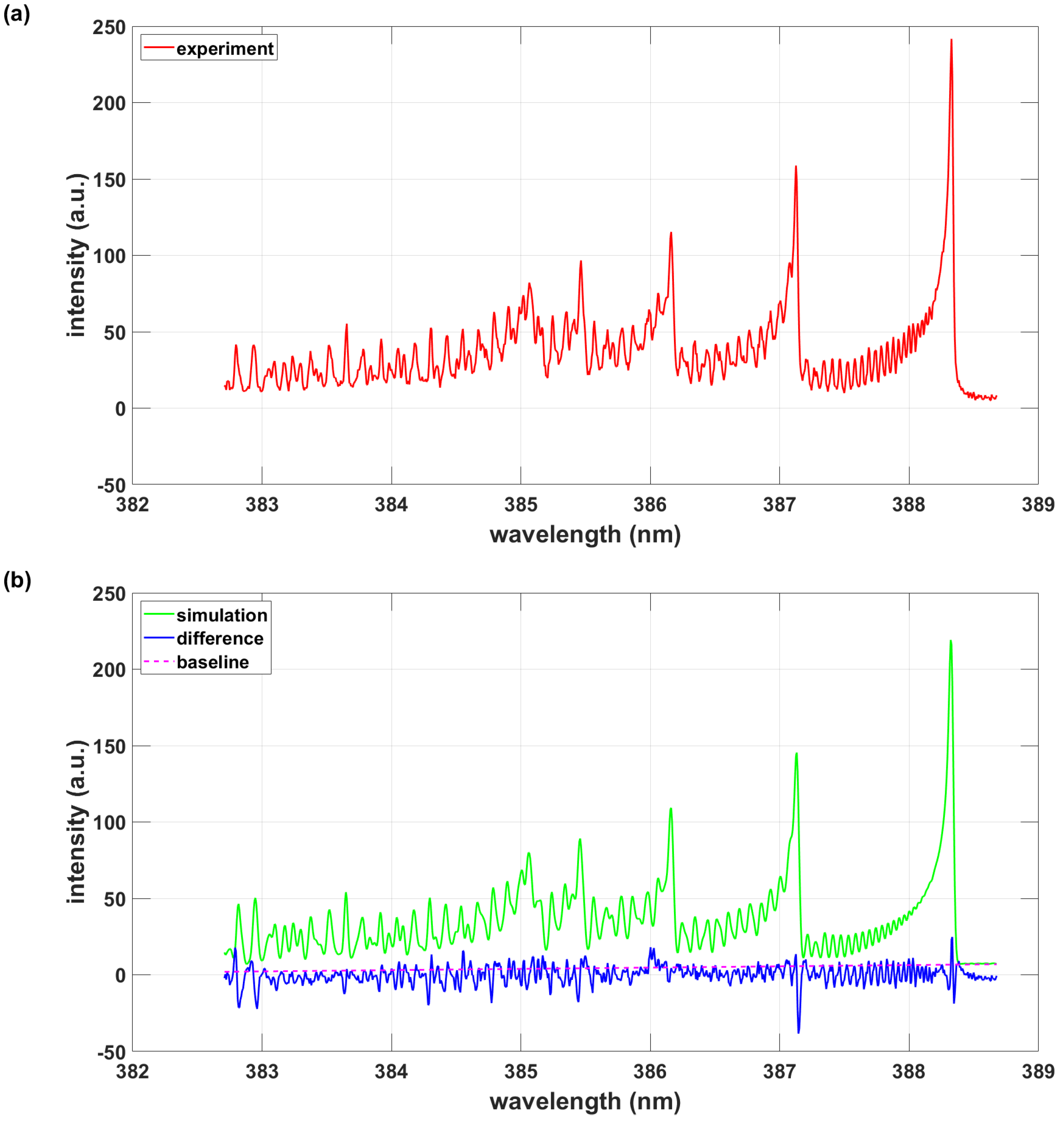
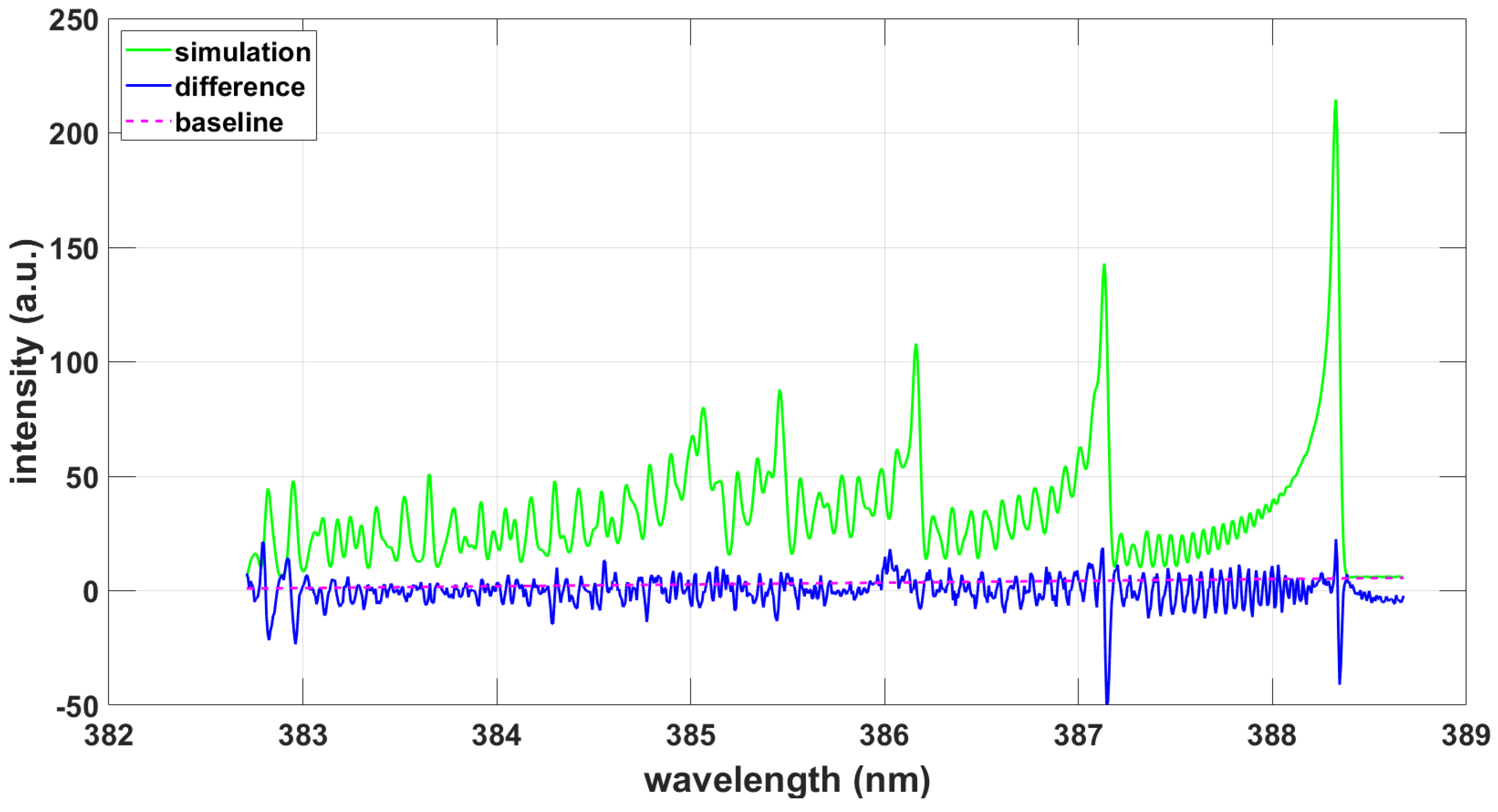
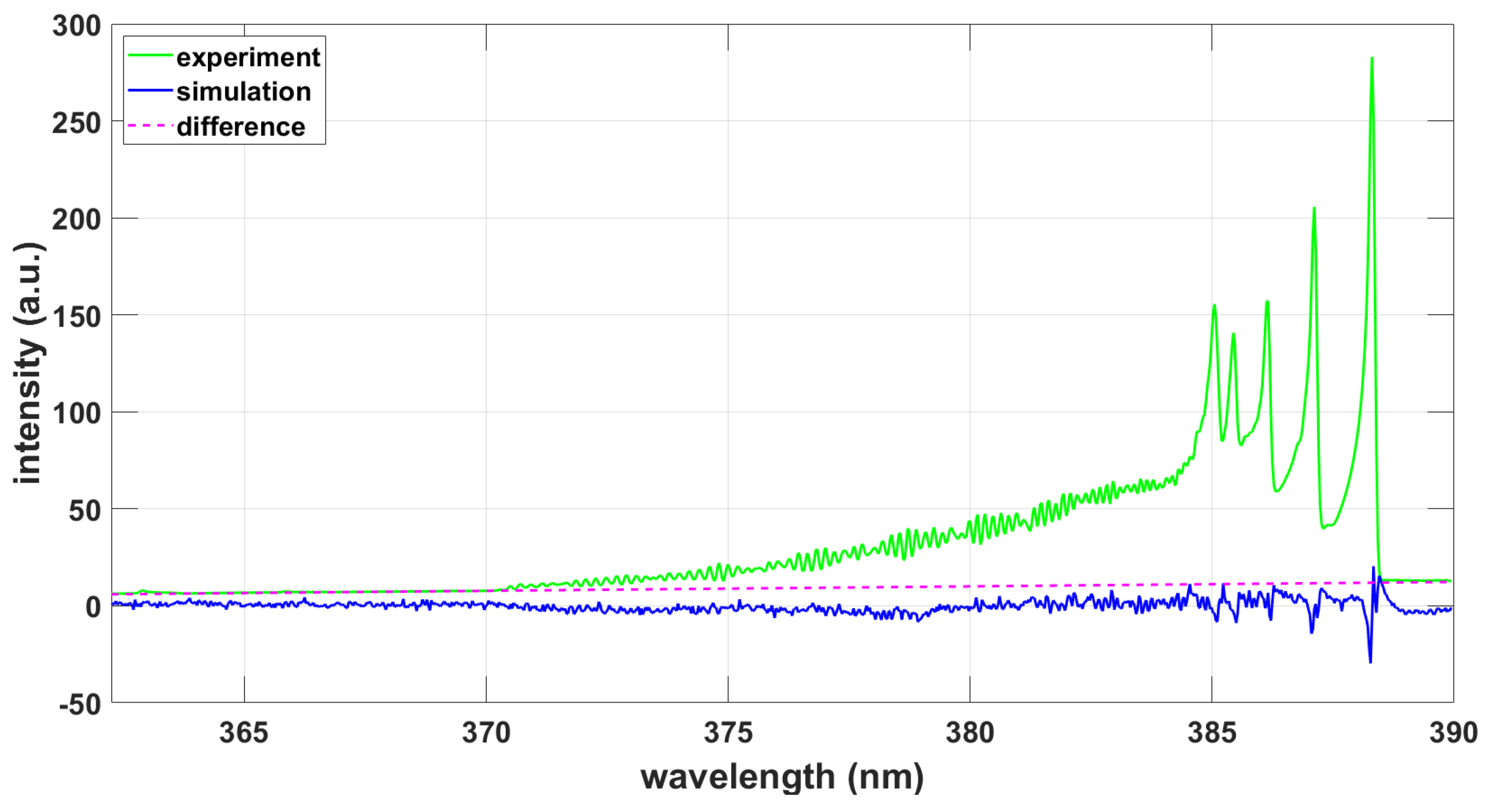
3.1.1. PGOPHER Program Using PGOPHER Data

The full CN B-X and A-X transition data are available for the construction of simulated spectra. Figure 1 displays measured and fitted CN violet spectra. The fitted spectrum also shows the baseline correction and difference between experimental and simulated spectra.

The synthetic spectrum is fitted using the PGOPHER program and an overlay of the experimental record of recorded optical multichannel analyzer (OMA) counts versus vacuum wavenumbers that are computed from the recorded air wavelengths.

Table 4. PGOPHER fitting parameters for the 0.033 nm data and results.

Parameter	Value	Standard Deviation
Temperature (K)	8103	187
Gaussian width (cm${}^{-1}$)	2.2	0.03
Scale (a.u.)	43,960	790
T${}_{\mathrm{vib}}$ (K)	8108	146

lists results for parameters that were selected for fitting. Normalized intensity units were used, i.e., the partition function is implemented. Following a separate fit for determination of the wavenumber offset of $-0.31$ cm${}^{-1}$ ($-0.005$ nm-the Doppler width at ≃8000 K for CN equals ≃ 0.005 nm), the selected parameters included Gaussian width, temperature, scaling, and T${}_{\mathrm{vib}}$ that assess deviation from thermodynamic equilibrium. The T${}_{\mathrm{vib}}$ results confirms Boltzmann distribution equilibrium within the standard deviation.

In this work, a Gaussian profile models the spectrometer and intensified linear-array detector transfer function. However, a measured system transfer function or a Voigt function can replace the selected Gaussian profile provided that changes are implemented in the MATLAB source scripts for the recently communicated BESP and NMT scripts [20]. The PGOPHER program allows one to accomplish Voigt profile fits.

Investigations of fitting Gaussian, $w_G$, and Lorentzian, $w_L$, widths, while leaving all other parameters constant, leads to the PGOPHER results $w_G=1.6{\mathrm{cm}}^{-1}$ (0.024 nm) and $w_L=0.64{\mathrm{cm}}^{-1}$ (0.0095 nm). Application of an empirical Voigt width, $w_V$, approximation [40],

$$w_V\approx w_L/2+\sqrt{w_L^2/4+w_G^2},$$

(14)

results in $w_V\approx 2.0{\mathrm{cm}}^{-1}$ (0.029 nm). The widths in units of nm that are indicated in brackets are calculated using $\Delta \mathsf{\lambda }=\Delta \tilde{\mathsf{\nu }}\times {\mathsf{\lambda }}^2$ at a wavelength of 386 nm (central wavelength of the 0.033 nm spectral resolution data). The Lorentzian contribution to the Voigt profile amounts to ≈30 per cent.

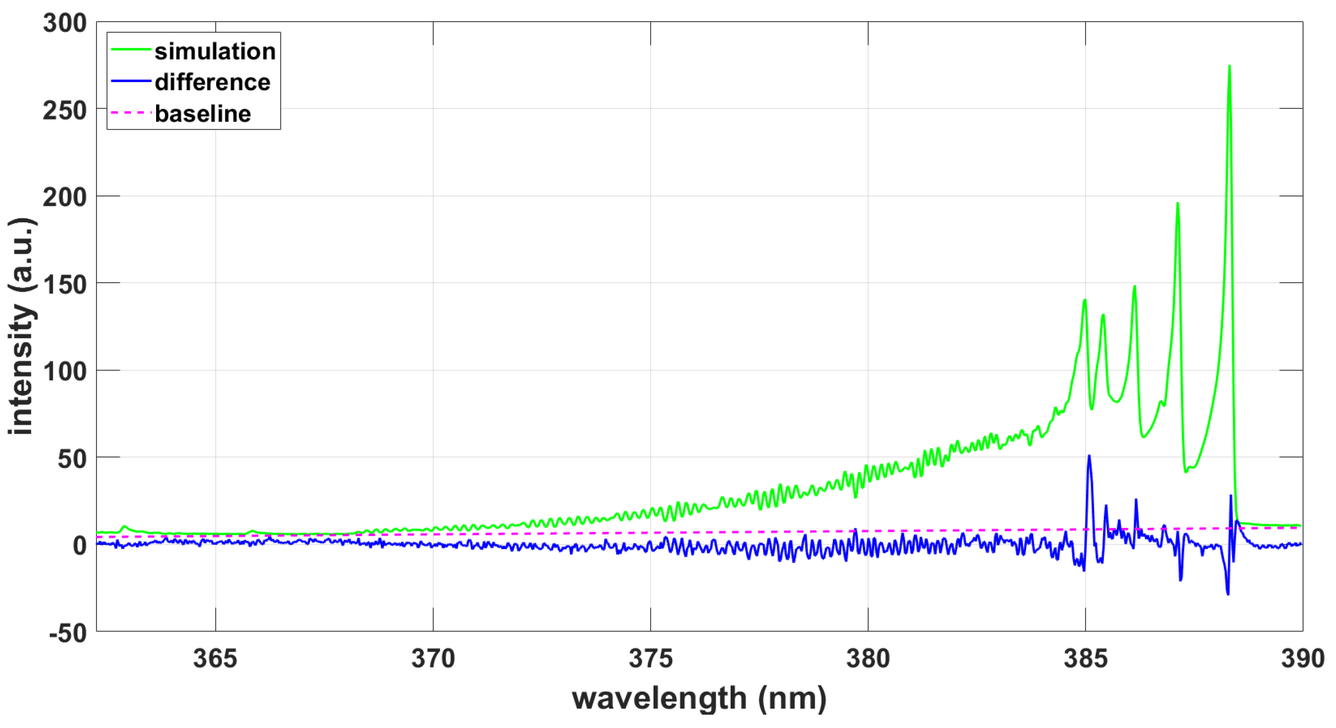
3.1.2. NMT Program Using PGOPHER and ExoMol Line Strengths

In addition, CN B-X line positions and Einstein A-coefficients (that are converted to line strengths) are collected in a data file that is compatible with the mentioned NMT spectral fitting program.

Figure 2 illustrates spectra determined from temperature and Gaussian line-width fitting. The results are consistent with those obtained from the versatile PGOPHER program. The inclusion of CN A-X data in the analysis would change the inferred temperature by ≃0.1%.

Similarly, the recommended ExoMol databases for states and transitions were utilized to generate a subset of lines and strength for analysis with the NMT program and for the 0.033 nm resolution data.

The results displayed in Figure 3 indicate a Gaussian full width at half maximum (FWHM) of 0.038 nm, indicative of line-position differences in the ExoMol data. However, the inferred temperature appears consistent with the results illustrated in Figure 1 and Figure 2.

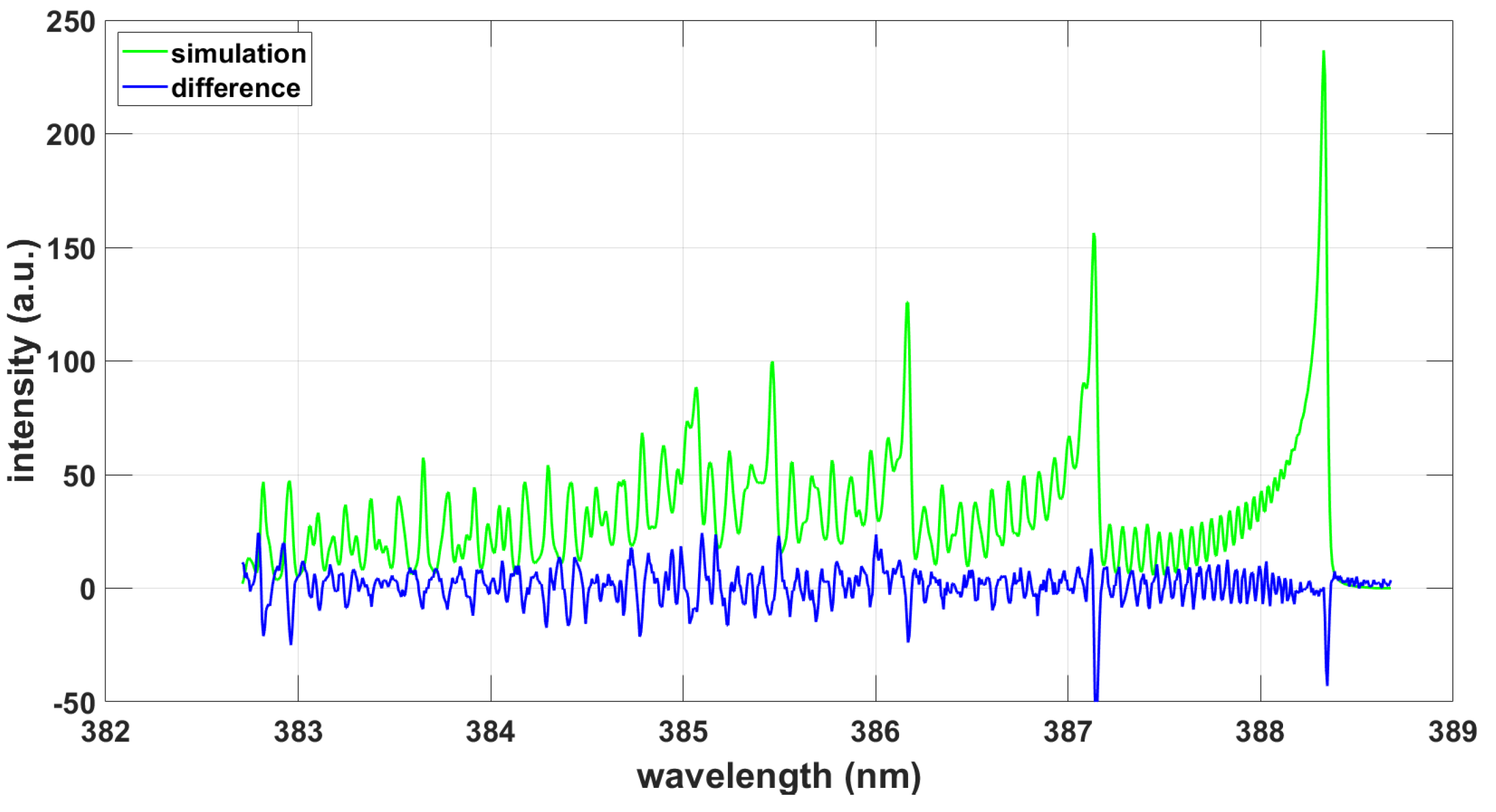
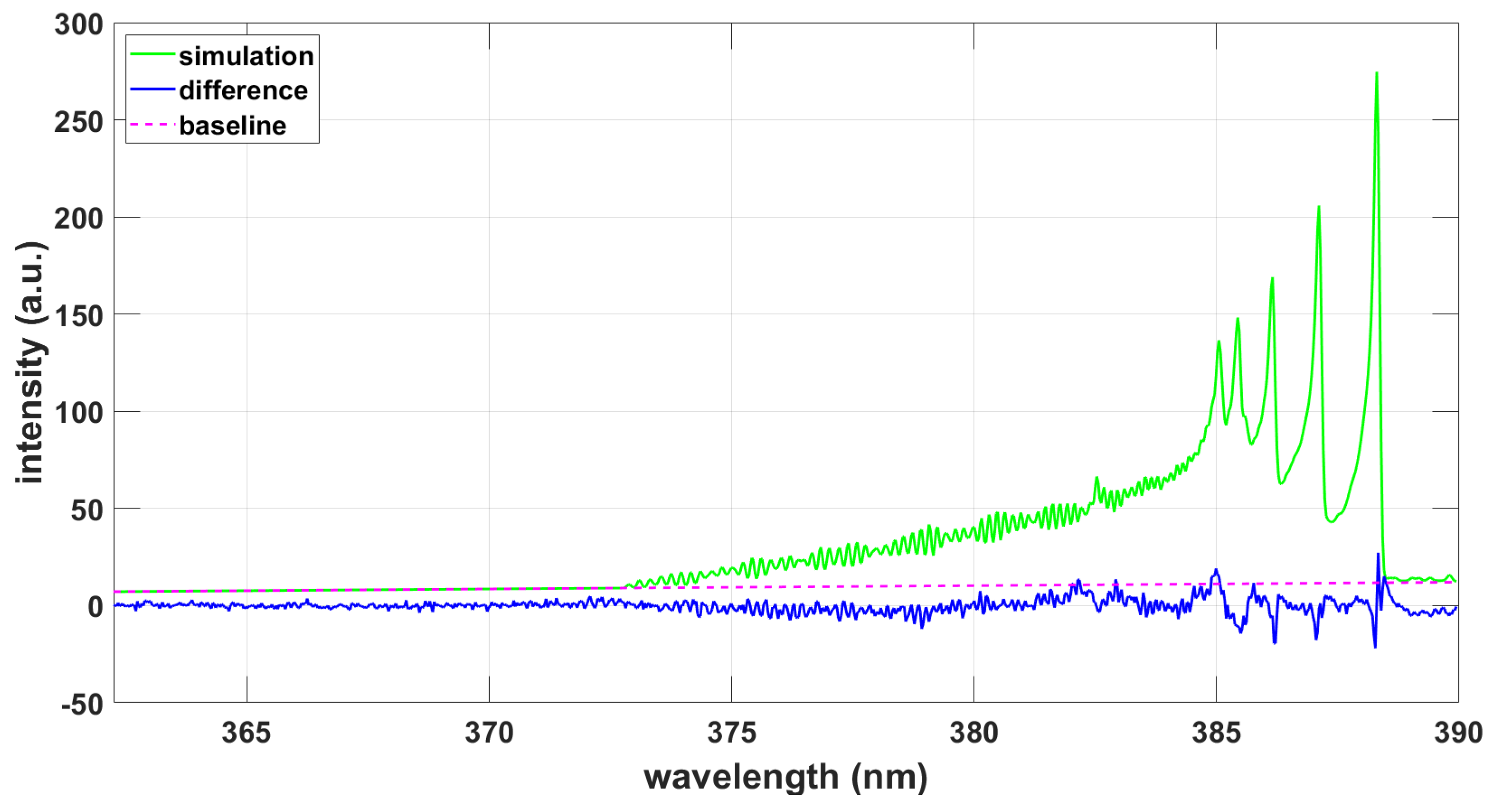
3.1.3. NMT Program Using CNv-lsf Data, Comparisons

Analysis of the measured data with the CNv-lsf data reveals a temperature of T = 8140 K and a fitted FWHM of 0.038 nm. Figure 4 shows the fitting results.

The simulated spectra in Figure 1, Figure 2, Figure 3 and Figure 4 display superposition spectra from quite a few individual rotational–vibrational transitions of the CN B-X $\Delta \mathrm{v}=0$ sequence. Actually, small contributions from the CN A-X transition are also included in the PGOPHER and ExoMol databases.

Table 5. Number of transitions of the simulated spectra in the measured experimental ranges for the 0.033 nm (25,725 ${\mathrm{cm}}^{-1}$ to 26,125 ${\mathrm{cm}}^{-1}$) data.

Database	0.033 nm Range CN B-X	0.033 nm Range CN B-X and A-X
PGOPHER	3598	5631
ExoMol	4302	17,181
CNv-lsf	2461	2461

and

Table 6. Number of transitions of the simulated spectra in the measured experimental ranges for the 0.033 nm data (see Table 5) with Einstein A-coefficients larger than 10${}^3$ s${}^{-1}$.

Database	0.033 nm Range CN B-X	0.033 nm Range CN B-X and A-X
PGOPHER	3205	4532
ExoMol	3625	8270
CNv-lsf	2461	2461

summarize the number of lines in the data files.

Comparisons of CN B-X line position accuracies in the PGOPHER and ExoMol databases with those of the CNv-lsf database are further elaborated for the range of the 0.033 nm resolution experiments (25,725 ${\mathrm{cm}}^{-1}$ to 26,125 ${\mathrm{cm}}^{-1}$) and for Einstein A-coefficients larger than 10${}^3$ s${}^{-1}$ (see first column in Table 6).

Table 7. Subset CN B-X lines of the PGOPHER and ExoMol data that agree within $\Delta \tilde{\mathsf{\nu }}$ of 2461 CN B-X transitions in the CNv-lsf data for the 0.033 nm range (25,725 ${\mathrm{cm}}^{-1}$ to 26,125 ${\mathrm{cm}}^{-1}$).

Database	$\mathbf{\Delta }\tilde{\mathsf{\nu }}$ < 0.05 ${\mathbf{cm}}^{-1}$	$\mathbf{\Delta }\tilde{\mathsf{\nu }}$ < 0.2 ${\mathbf{cm}}^{-1}$	$\mathbf{\Delta }\tilde{\mathsf{\nu }}$ < 1.0 ${\mathbf{cm}}^{-1}$	$\mathbf{\Delta }\tilde{\mathsf{\nu }}$ < 2.0 ${\mathbf{cm}}^{-1}$
PGOPHER	1200	1422	1823	2012
ExoMol	158	463	1266	1935

displays agreements of lines within the indicated wavenumber range and otherwise the same angular momentum values for upper and lower levels of the transitions.

Various aspects of the accuracy of the CNv-lsf database have been extensively tested [19], including analysis of laser-induced fluorescence and nominal 300 K temperature Fourier transform spectra. The differences in predictions for line positions appear larger for levels with higher angular momenta, $J^{\prime }$ and J. The accuracy of line positions in the CNv-lsf database is better than 0.05 ${\mathrm{cm}}^{-1}$. Table 7 reveals that PGOPHER line positions compare favorably with those in the CNv-lsf database. The ExoMol database appears acceptable within ≃2 wavenumbers that correspond to a spectral resolution of ≃0.033 nm. However, high-temperature (≃8,000 K) inferences from CN B-X spectra at a 0.033 nm experimental spectral resolution appear only minimally affected (see Figure 2 and Figure 3).

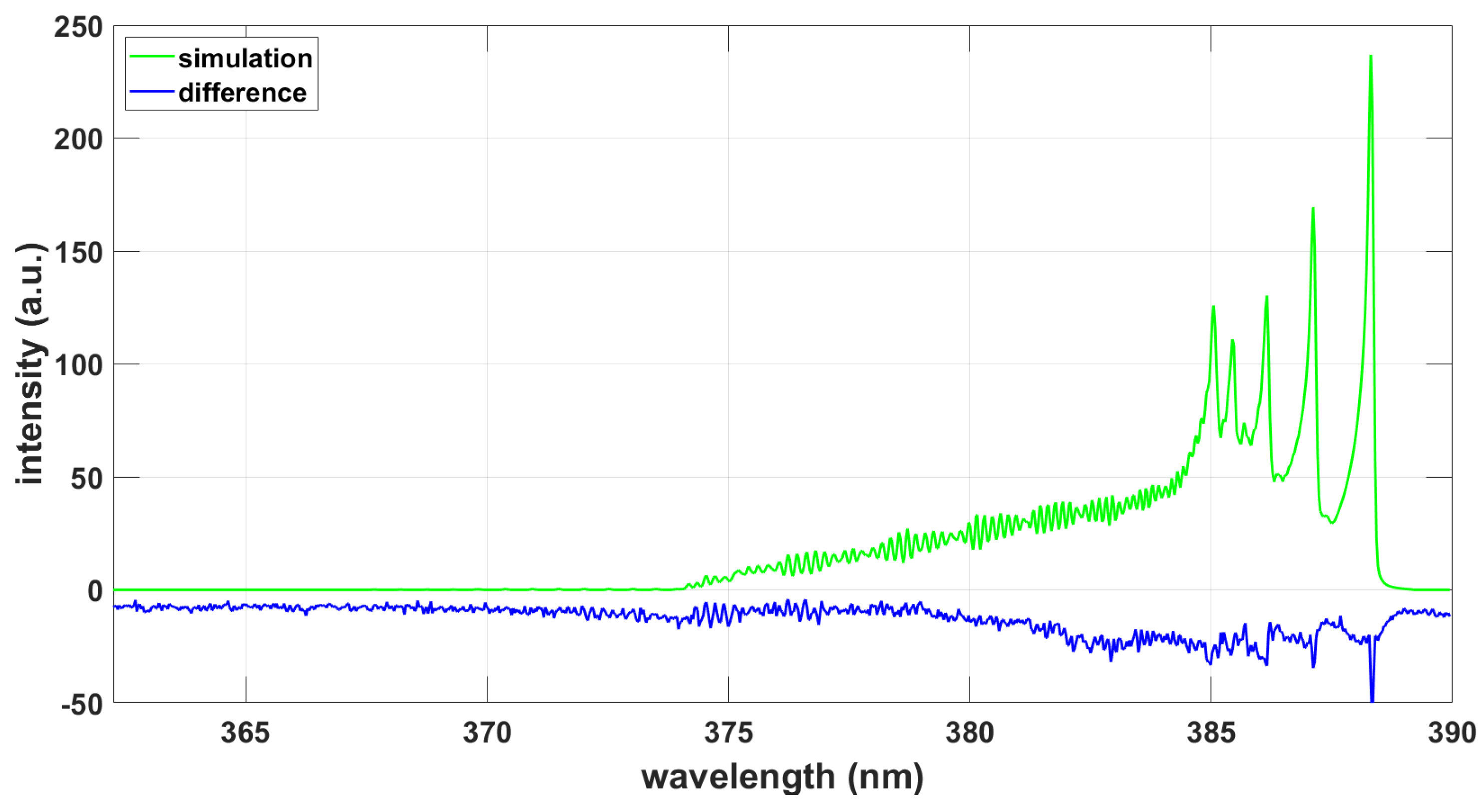
3.1.4. LIFBASE Program

The LIFBASE program is also used for simulation of the measured spectrum. A Voigt profile of width 0.033 nm with a 30% Lorentzian contribution is selected. Figure 5 illustrates the results. Noteworthy is that the PGOPHER program is capable of fitting Voigt profiles as well. However, Gaussian profiles are usually selected in the NMT program for modeling of the spectrometer and detector transfer function. The choice of a 30% Lorentzian contribution is based on PGOPHER-program investigations, see Equation (14).

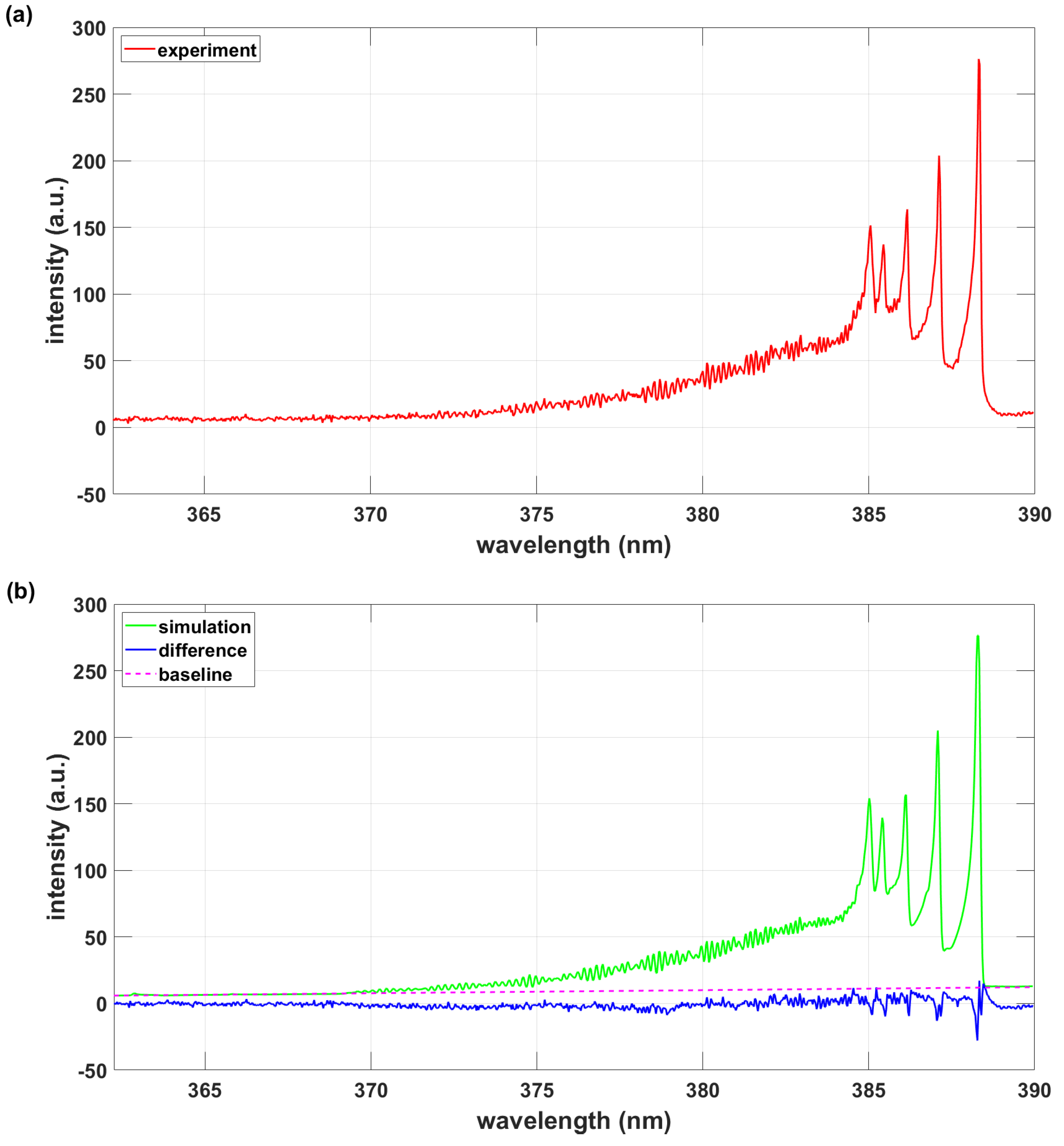
3.2. Analysis of the 0.11 nm Spectral Resolution Data

The lower resolution 0.11 nm data are analyzed using a similar approach as that for the 0.033 nm data. It is noteworthy that the recorded average spectra for both lower and higher resolution show coincidentally similar detector counts (or intensity in arbitrary units) for the two different gratings, respectively.

3.2.1. PGOPHER Program Using PGOPHER Data

Following a separate fit for determination of the wavenumber offset of 0.13 cm${}^{-1}$ (0.002 nm), the selected parameters included Gaussian width, temperature, and scaling. Figure 6 illustrates the results obtained by employing the PGOPHER fitting program and the available full CN B-X and CN A-X data set [32]. The effect of the CN A-X transition lines is minimal for temperature inference, viz., 0.1% for the higher spectral resolution data (see Figure 2).

Table 8. PGOPHER fitting parameters for the 0.11 nm data and results.

Parameter	Value	Standard Deviation
Temperature (K)	8340	43
Gaussian width (cm${}^{-1}$)	7.1	0.07
Scale (a.u.)	107,300	850

summarizes the results of PGOPHER fitting including the standard deviations.

3.2.2. NMT Program Using PGOPHER and ExoMol Line Strengths

Figure 7 displays the results of the NMT program using PGOPHER data. As before, the NMT program resorts to fitting of relative intensities. In turn, the scales that are indicated in Table 4 and Table 8 can serve as a calibration of the detector counts in the laboratory-recorded CN spectra.

The fitting of the experimental data using the PGOPHER-extracted wavenumbers, upper term values, and Einstein A-coefficients (that are converted to line strengths) with the NMT program shows similar results as obtained for exclusive PGOPHER fitting.

Fitting the ExoMol data using the NMT program yields a temperature of T = 9090 K for a spectral resolution of $\Delta \mathsf{\lambda }=0.11\mathrm{nm}$. Figure 8 illustrates the simulated spectrum, difference and baseline.

3.2.3. NMT Program Using CNv-lsf Data, Comparisons

A temperature of T = 8940 K is obtained when using CNv-lsf in the NMT program. Figure 9 shows the results.

Table 9. Number of transitions of the simulated spectra in the measured experimental ranges for the 0.11 nm (25,600 ${\mathrm{cm}}^{-1}$ to 27,600 ${\mathrm{cm}}^{-1}$) data.

Database	0.11 nm Range CN B-X	0.11 nm Range CN B-X and A-X
PGOPHER	7115	14,349
ExoMol	10,499	78,079
CNv-lsf	3313	3313

and

Table 10. Number of transitions of the simulated spectra in the measured experimental ranges for the 0.11 nm data (see Table 9) with Einstein A-coefficients larger than 10${}^3$ s${}^{-1}$.

Database	0.11 nm Range CN B-X	0.11 nm Range CN B-X and A-X
PGOPHER	6187	9958
ExoMol	8259	28,274
CNv-lsf	3313	3313

summarize the number of lines in the data files.

3.2.4. LIFBASE Program

Similar to the higher resolution data, the LIFBASE program is utilized for the generation of a simulated spectrum. Again, a 30% Lorentzian contribution is selected based on the investigations with Gaussian and Lorentzian profile contributions, see Equation (14). Figure 10 displays the results.

4. Discussion

The CN violet $B{}^2{\Sigma }^{+}-X{}^2{\Sigma }^{+}$, $\Delta \mathrm{v}=0$ sequence reveals a multitude of vibrational and rotational transitions that are usually not individually resolved in the study of laser-induced plasma emissions in the spectral range of 383 nm to 389 nm. Analysis of the 0.033 nm spectral resolution experimental emission spectrum with the PGOPHER program and use of a full CN B-X data file yields CN excitation temperature of ≃ 8100 K and a standard deviation of ≃ 200 K.

Similar results were obtained when using the CN B-X data in conjunction with a Nelder–Mead spectral fitting program. The most recent ExoMol CN data also predict a temperature within the standard deviation of the PGOPHER prediction, but there appear to be discrepancies in the ExoMol predictions near the 2-2, 3-3, and 4-4 band heads or in the range of 385 nm to 386 nm. Analogous results are noted when using the CNv-lsf line strengths, however with slightly better agreement of experimental and simulated spectra than those for ExoMol. Comparative spectra obtained from the LIFBASE program are also largely in agreement with the measured data.

The lower 0.11 nm resolution data in the range of 362 nm to 390 nm appear to be well predicted by the PGOPHER data. About 6% higher temperatures are predicted with the ExoMol and the CNv-lsf data. The CN violet spectra have been extensively tested in a variety of experimental studies of laser plasma.

For comprehensive comparisons of experimental and simulated spectra, however, the higher the spectral resolution the better. The expansive PGOPHER and ExoMol line lists allow one to predict simulated spectra consistent with laboratory laser–plasma experiments.

References

1. Roth, K.C.; Meyer, D.M.; Hawkins, I. Interstellar cyanogen and the temperature of the cosmic microwave background radiation. Astrophys. J. 1993, 413, L67–L71. [Google Scholar] [CrossRef]
2. Leach, S. CN spectroscopy and cosmic background radiation measurements. Can. J. Chem. 2004, 82, 730–739. [Google Scholar] [CrossRef]
3. Ram, R.S.; Davis, S.P.; Wallace, L.; Englman, R.; Appadoo, D.R.T.; Bernath, P.F. Fourier transform emission spectroscopy of the B2Σ+-X2Σ+ system of CN. J. Mol. Spectrosc. 2006, 37, 225–231. [Google Scholar] [CrossRef]
4. Brooke, J.S.A.; Ram, R.S.; Western, C.M.; Li, G.; Schwenke, D.W.; Bernath, P.F. Einstein A Coefficients and Oscillator Strengths for the A2Π-X2Σ+ (Red) and B2Σ+-X2Σ+ (Violet) Systems and Rovibrational Transitions in the X2Σ+ State of CN. Astrophys. J. Suppl. Ser. 2014, 210, 1–15. [Google Scholar] [CrossRef] [Green Version]
5. Davis, S.P. Laboratory spectrsoscopy of astrophysically interesting molecules. Publ. Astron. Soc. Pac. 1987, 99, 1105–1114. [Google Scholar] [CrossRef]
6. Kunze, H.-J. Introduction to Plasma Spectroscopy; Springer: Berlin/Heidelberg, Germany, 2009. [Google Scholar]
7. Fujimoto, T. Plasma Spectroscopy; Clarendon Press: Oxford, UK, 2004. [Google Scholar]
8. Ochkin, V.N. Spectroscopy of Low Temperature Plasma; Wiley-VCH: Weinheim, Germany, 2009. [Google Scholar]
9. Demtröder, W. Laser Spectroscopy 1: Basic Principles, 5th ed.; Springer: Berlin/Heidelberg, Germany, 2014. [Google Scholar]
10. Demtröder, W. Laser Spectroscopy 2: Experimental Techniques, 5th ed.; Springer: Berlin/Heidelberg, Germany, 2015. [Google Scholar]
11. Miziolek, A.W.; Palleschi, V.; Schechter, I. (Eds.) Laser Induced Breakdown Spectroscopy (LIBS): Fundamentals and Applications; Cambridge Univ. Press: New York, NY, USA, 2006. [Google Scholar]
12. Singh, J.P.; Thakur, S.N. (Eds.) Laser-Induced Breakdown Spectroscopy, 2nd ed.; Elsevier: Amsterdam, The Netherlands, 2020. [Google Scholar]
13. Tennyson, J.; Yurchenko, S.N.; Al-Refaie, A.F.; Clark, V.H.J.; Chubb, K.L.; Conway, E.K.; Dewan, A.; Gorman, M.N.; Hill, C.; Lynas-Gray, A.E.; et al. The 2020 release of the ExoMol database: Molecular line lists for exoplanet and other hot atmospheres. J. Quant. Spectrosc. Radiat. Transf. 2020, 255, 107228. [Google Scholar] [CrossRef]
14. Luque, J.; Crosley, D.R. LIFBASE: Database and Spectral Simulation for Diatomic Molecules. 2021. Available online: https://www.sri.com/platform/lifbase-spectroscopy-tool (accessed on 25 November 2019).
15. Western, C.M. PGOPHER, A Program for Simulating Rotational, Vibrational and Electronic Spectra. J. Quant. Spectrosc. Radiat. Transf. 2017, 186, 221–242. [Google Scholar] [CrossRef] [Green Version]
16. McKemmish, L.K. Molecular diatomic spectroscopy data. WIREs Comput. Mol. Sci. 2021, 11, e1520. [Google Scholar] [CrossRef]
17. Rothman, L.S.; Gordon, I.E.; Barber, R.J.; Dothe, H.; Gamache, R.R.; Goldman, A.; Perevalov, V.I.; Tashkun, S.A.; Tennyson, J. HITEMP, the high-temperature molecular spectroscopic database. J. Quant. Spectrosc. Radiat. Transf. 2010, 111, 2139–2150. [Google Scholar] [CrossRef]
18. MATLAB Release R2022a Update 5; The MathWorks, Inc.: Natick, MA, USA, 2022.
19. Parigger, C.G.; Hornkohl, J.O. Quantum Mechanics of the Diatomic Molecule with Applications; IOP Publishing: Bristol, UK, 2020. [Google Scholar]
20. Parigger, C.G. Diatomic line strengths for fitting selected molecular transitions of ALO, C2, CN, OH, N2+, NO, and TiO, spectra. Foundations 2023, 3, 1–15. [Google Scholar] [CrossRef]
21. Hornkohl, J.O.; Parigger, C.G.; Lewis, J.W.L. Temperature Measurement from CN spectra in a laser-induced plasma. J. Quant. Spectrosc. Radiat. Transf. 1991, 46, 405–411. [Google Scholar] [CrossRef]
22. Dunham, J.L. The Energy Levels of a Rotating Vibrator. Phys. Rev. 1932, 41, 721–731. [Google Scholar] [CrossRef]
23. National Institute of Standards and Technology (NIST) Chemistry WebBook, SRD 69, for the Cyano Radical, Constants of Diatomic Molecules. 2021. Available online: https://webbook.nist.gov (accessed on 20 February 2023).
24. Whiting, E.E.; (Space Administration, Reacting Flow Environments Branch, Ames Research Center, CA, USA). Personal communication, 1995.
25. Whiting, E.E.; Park, C.; Liu, Y.; Arnold, J.; Paterson, J. NEQAIR96, Nonequilibrium and Equilibrium Radiative Transport and Spectra Program: User’s Manual; Technical Report NASA RP-1389; NASA Ames Research Center: Moffet Field, CA, USA, 1996. [Google Scholar]
26. Boulous, P.M.I.; Pfender, E. Thermal Plasmas-Fundamentals and Applications; Plenum Press: New York, NY, USA, 1994. [Google Scholar]
27. McBride, B.; Gordan, S. Interim Revision NASA Report RP-1311, Part I; NASA Lewis Research Center: Cleveland, OH, USA, 1994. [Google Scholar]
28. McBride, B.; Gordan, S. Interim Revision NASA Report RP-1311, Part II; NASA Lewis Research Center: Cleveland, OH, USA, 1996. [Google Scholar]
29. Laux, C.O. Radiation and Nonequilibrium Collisional-Radiative Models, von Karman Institute Lecture Series 2002-07, Physico-Chemical Modeling of High Enthalpy and Plasma Flows; Fletcher, D., Charbonnier, J.-M., Sarma, G.S.R., Magin, T., Eds.; Rhode-Saint-Genèse: Flanders, Belgium, 2002. [Google Scholar]
30. Syme, A.-M.; McKemmish, L.K. Experimental energy levels of 12C14N through MARVEL analysis. Mon. Not. R. Astron. Soc. 2020, 499, 25–39. [Google Scholar] [CrossRef]
31. Syme, A.M.; McKemmish, L.K. Full spectroscopic model and trihybrid experimental-perturbative-variational line list for CN. Mon. Not. R. Astron. Soc. 2021, 505, 4383–4395. [Google Scholar] [CrossRef]
32. Western, C.M.; (University of Bristol, Bristol, UK). Personal communication, 2019.
33. Condon, E.U.; Shortley, G.H. The Theory of Atomic Spectra; Cambridge Univ Press: Cambridge, UK, 1964. [Google Scholar]
34. Hilborn, R.C. Einstein coefficients, cross sections, f values, dipole moments, and all that. Am. J. Phys. 1982, 50, 982–986. [Google Scholar] [CrossRef] [Green Version]
35. Thorne, A.P. Spectrophysics, 2nd ed.; Chapman and Hall: New York, NY, USA, 1988. [Google Scholar]
36. Wigner, E.; Witmer, E.E. Über die Struktur der zweiatomigen Molekelspektren nach der Quantenmechanik. Z. Phys. 1928, 51, 859–886. [Google Scholar] [CrossRef]
37. Wigner, E.; Witmer, E.E. On the structure of the spectra of two-atomic molecules according to quantum mechanics. In Quantum Chemistry: Classic Scientific Papers; Hettema, H., Ed.; World Scientific: Singapore, 2000; pp. 287–311. [Google Scholar]
38. Barrell, H.; Sears, J.E. The Refraction and Dispersion of Air for the Visible Spectrum. Philos. Trans. R. Soc. 1939, 238, 1–64. [Google Scholar]
39. Ciddor, P.E. Refractive index of air: New equations for the visible and near infrared. Appl. Opt. 1996, 35, 1567–1573. [Google Scholar] [CrossRef]
40. Whiting, E.E. An empirical approximation to the Voigt profile. J. Quant. Spectrosc. Radiat. Transf. 1968, 8, 1379–1384. [Google Scholar] [CrossRef]
Figure 1. (a) Experimental spectrum; (b) simulation with PGOPHER, T = 8103 K, Δ λ = 0.033 nm .
Atoms 11 00062 g001
Figure 2. Simulation using PGOPHER data and the NMT program, T = 8240 K, Δ λ = 0.034 nm .
Atoms 11 00062 g002
Figure 3. Simulation using ExoMol data and the NMT program, T = 8150 K, Δ λ = 0.038 nm .
Atoms 11 00062 g003
Figure 4. Simulation using CNv-lsf data and the NMT program, T = 8140 K, Δ λ = 0.036 nm .
Atoms 11 00062 g004
Figure 5. Simulation using LIFBASE with fixed T = 8103 K, Δ λ = 0.033 nm , Voigt profile with 30% Lorentzian contribution.
Atoms 11 00062 g005
Figure 6. (a) Experimental spectrum; (b) simulation with PGOPHER, T = 8340 K, Δ λ = 0.11 nm .
Atoms 11 00062 g006
Figure 7. Simulation using PGOPHER data and the NMT program, T = 8380 K, Δ λ = 0.11 nm .
Atoms 11 00062 g007
Figure 8. Simulation using ExoMol data and the NMT program, T = 9090 K, Δ λ = 0.11 nm .
Atoms 11 00062 g008
Figure 9. Simulation using CNv-lsf data and the NMT program, T = 8940 K, Δ λ = 0.11 nm .
Atoms 11 00062 g009
Figure 10. Simulation using LIFBASE with fixed T = 8340 K, Δ λ = 0.11 nm , Voigt profile with 30% Lorentzian contribution.
Atoms 11 00062 g010